1. Introduction
Cirrus clouds are thin and wispy clouds which are entirely made of ice [
1]. They form in very cold air at high altitudes in the range from 7 km to 20 km. They are common high clouds which can be seen at any time during the year. They are found generally in the Upper Troposphere/Lower Stratosphere (UTLS) region, and most of the regions of these clouds are composed of non-spherical ice crystals.
The presence of these clouds increases the fraction of the solar radiation reflected back to space known as the solar albedo effect. On the other hand, these clouds absorb outgoing thermal radiation from the earth known as the infrared greenhouse effect [
2]. Both of these phenomena affect the Earth’s radiation and climate, the former leading to a cooling of the system and later to the warming of the system [
3]. Few climate modeling studies reported that a warming climate could greatly influence the earth’s atmosphere and that would vary rapidly based on the geometrical properties of cirrus clouds [
4,
5]. As a result, a clear understanding of cirrus cloud parameterization in terms of their occurrence characteristics, geometrical, and optical characteristics at distinctive geographical areas are highly essential for regional and global climate modeling studies. These studies are useful in the Generation Circulation Models (GCM’s) because of their significant role in the radiative balance, climate, and exchange of water vapor.
The cirrus cloud characteristics include geometrical properties (base, mid, and top heights, and thickness) and optical properties (depolarization ratio and optical depth). A statistical technique referred to as the Variance Centroid Method (VCM) or the Variance Method (VM) is employed to determine these geometrical and optical properties. The seasonal, monthly, and statistical variations of the properties of tropical cirrus clouds are also studied by the measuring instrument. The purpose of this study is mainly to analyze the characteristics of cirrus clouds and their statistics for the given period of observation.
VCM is primarily suited for the precise determination of Atmospheric Boundary Layer (ABL) structures with respect to different altitudes over dynamic environmental regions. It has the greatest magnitude and is more sensitive (for clouds also) even to the tiny fluctuations of the lidar backscattered signal. In the present work, an attempt has been made to apply VCM to cirrus cloud datasets to determine the cloud’s base, mid, and top heights. The VCM approach is useful in detecting the deviation of the minimum, peak, and maximum signals of the cirrus cloud. It also directly indicates the boundaries of the cirrus cloud and provides information on its geometrical characteristics with high spatial and temporal resolutions. Most of the methods used in this study to retrieve the cirrus cloud boundary altitudes are relevant to the geometrical characteristics of the cirrus cloud from the lidar backscatter signals under different meteorological conditions. It can lead to varied atmospheric conditions on the macroscopic or geometrical properties of cirrus clouds, their extent, lifetime, and radiative properties which are of great interest in the study of cirrus cloud-climate.
2. Site and Instrument Description
2.1. Area of Study
Gadanki (13.5° North, 79.2° East) is a rural observational site which is also a tropical hill station located in Andhra Pradesh, South India and is situated at an altitude of 375 m Above Mean Sea Level (AMSL). This location is surrounded by small hills with changeable altitudes of around 200 m–300 m Above Ground Level (AGL) and is also encircled by forest and farming fields to a radius of 1 km [
6]. The surface meteorology conditions [
7] and the atmospheric weather conditions of this site have strong seasonal variations [
8]. A detailed description of the background (weather, topographical, and meteorological) conditions over this region were reported by [
6]. The atmosphere over Gadanki is generally clear during the months of January to March and the rainy seasons in the months of July to November. To analyze the properties of cirrus cloud for the present study, the prominent seasons were divided into four in a year as follows: (a) pre-monsoon (summer): March–April–May (MAM), (b) monsoon: June–July–August (JJA), (c) post-monsoon: September–October–November (SON) and (d) winter: December–January–February (DJF). The map (Indian subcontinent) location of Gadanki is shown in
Figure 1, and the cyan colored circle indicates the 50 km radius of this region.
2.2. Instrumentation Technique
LIDAR (LIght Detection And Ranging) is a powerful remote sensing technique used to probe and study the atmospheric structure and dynamics with high spatial and temporal resolutions. To study the atmospheric temperature (30–80 km), tropospheric aerosols (4–40 km), and clouds (4–20 km) in the Upper Troposphere and Lower Stratosphere (UTLS) region, a monostatic biaxial dual polarization lidar system was installed at the National Atmospheric Research Laboratory (NARL), Gadanki (13.5° N; 79.2° E), a tropical region over the Indian subcontinent. Since January 2007, a new laser source (transmitter) was used instead of the earlier laser source (from March 1998–December 2006). It employs a doubled frequency Neodymium: Yttrium Aluminum Garnet (Nd: YAG) pulsed laser source as the transmitter and two telescopes as the receiver. The new laser unit system uses the second harmonic output at 532 nm wavelength with a pulse repetition frequency of 50 Hz. Each laser pulse-width has duration of 7ns with a maximum energy of about 600 mJ per pulse [
9].
The Lidar system employs two independent telescopes to collect Rayleigh and Mie backscattered signals. The Rayleigh receiver (Newtonian type telescope; 750 mm diameter; Field Of View (FOV) is 1mrad) collects the backscattered light from air molecules, which is used to study the middle atmospheric temperature in the range of 30 km to 80 km. The Mie receiver (Schmidt–Cassegrain type telescope; 350 mm diameter; Field Of View (FOV) 1mrad) is used for collecting the backscattered light from the particles and clouds, which is used to study the altitude formation of atmospheric clouds employing both the scattered signals of Rayleigh and Mie in the range of 4 to 40 km. To suppress the unwanted signals from the background radiation, a narrow-band (1.13 nm FWHM, a center wavelength of 532 nm) interference filter was used in front of the polarizing beam splitter. In the Mie receiver, the polarizing beam splitter splits the beam into cross-polarized and co-polarized signal components. This Mie receiver is capable of dual polarization diversity and depolarization measurements. Both components are recorded separately by using the two identical and independent Photo Multiplier Tube (PMT) channels, which are designated as P (Co-polar) and S (Cross-polar) channels, respectively. The LIDAR utilizes photon-counting detector electronics such as the Philips-make pulse discriminators (300 MHz) and a PC-based data acquisition system called the Multi-Channel Scalar (MCS) add-on card. The MCS-records 12500 laser shots averaged photon count profiles as one frame with a time resolution of 250 sec. The photon count profiles from both the channels are acquired with dwell time (range bin width) of 2 µs (corresponds to 300 m resolution per range bin) for a range of 1024 bins. In a time frame of four minutes, one cirrus cloud lidar profile shall be generated, and hence, a few hours of measurement time often results in a large number of lidar profiles. In this computation, the distance between the laser beam and telescope is kept at 2 m.
3. Data Analysis
The lidar backscattered signal is optically received in terms of photon count signals. At first, these photon count profiles are corrected for the unwanted background signal counts and then normalized with the range. The received backscattered signal contains both scatterings from clouds (cirrus clouds if present) and aerosols. The lidar data are analyzed by employing the Fernald’s algorithm [
10] on the basis of the LIDAR equation:
where
is the lidar received power from the volume scattering at a slant height
,
is the output transmitted energy per laser pulse,
(
) is the overall efficiency of the lidar transmitter and receiver,
is the length of the volume illuminated by the laser pulse at a fixed time, and
appears because of the apparent folding of the laser pulse through the backscatter process,
is the primary area of the telescope,
and
are the backscattering and extinction coefficients at the laser wavelengths.
3.1. Scattering Ratio, Depolarization Ratio, and Optical Depth
The two quantities and in the Equation (1) consist of parts of the atmosphere as well as the cloud and are given by and , where and represent aerosol and molecular, respectively.
In general, the cloud and aerosol measurements for the lidar are represented in terms of the Scattering Ratio (SR),
is given as:
where
is the height,
and
are the aerosol and molecular backscattering coefficients. Scattering Ratio (SR) is used to separate the molecular and aerosol contributions in the lidar backscattered signal and it is achieved by the normalized photon counts with the molecular profile obtained from the radiosonde measurements. The obtained altitude profiles of
for the P and S channels are used to identify the presence of cirrus clouds in the altitude region of ~7 km–20 km. A threshold criterion [
11] is followed for the determination of cirrus clouds throughout the data analysis.
The Depolarization Ratio (DR) altitude profile is expressed in terms of scattering ratios of cross-polarized and co-polarized components, respectively. The scattering ratio of the cross-polarized component (
) to that of the co-polarized component (
) of the lidar backscattered signal with respect to height
is referred to as DR, denoted by
, and is written as:
The combined measured values of SR and DR are typically used to identify the composition of the clouds. The ice crystals with different shapes and water droplets present in the clouds can be distinguished by SR and DR values. These are the two important quantities which help in the analysis of cloud formation and dynamics [
12].
From the scattering theory of Rayleigh, the molecular scattering parameters
and
are given as
. The other parameters for the cloud are unknown but are related to the lidar ratio, a constant, derived using the lidar equation and it also determines the optical depth of the cirrus clouds. High altitude tropical cirrus clouds are classified based on the Cloud Optical Depth (COD),
defined as the opacity of the cloud and is given by:
where
is the extinction coefficient of the cirrus cloud, and
and
are the lower and upper boundaries of the cirrus cloud heights. It is also a measure of the extinction coefficient and mainly depends on the vertical thickness of a cloud [
13]. It relates to the opacity of the clouds and is evaluated by integrating the extinction coefficient within the boundaries of the cloud. The observed cirrus clouds are classified based on their COD into three types of categories, (i) COD < 0.03 referred to as sub-visual cirrus, (ii) 0.03 < COD < 0.3 referred to as thin cirrus, and (iii) COD > 0.3 (thick or dense or opaque cirrus) [
14,
15,
16].
3.2. Cirrus Cloud Detection
In the present study, the most versatile statistical method called the Variance Method (VM) or the Variance Centroid Method (VCM) [
17,
18,
19] is used to determine the base and top heights of the cirrus clouds. Earlier this method was developed to find the top of the atmospheric boundary layer [
20] in the altitudes of ~5 km. In the present work, this method is used for the detection of the base and top heights of the cirrus clouds. This method requires a minimum of three lidar signal profiles and a maximum of fifteen lidar signal profiles for averaging from the Mie lidar dataset and is used to estimate the top and base heights of cirrus clouds. This is due to the inconsistent nature of the cirrus clouds in the vertical atmosphere. The temporal resolution is also limited in this method for the determination of the top and base of the cirrus clouds. The backscatter variance is calculated from the temporal fluctuations of the lidar Range Corrected Signal (RCS) at each altitude [
19] given by
where
is the variance profile of RCS is,
is given by number of profiles,
is the range corrected signal and
is the mean of the range corrected signal.
In VCM, the detection of the base and top of the cirrus clouds is mainly based on the strength of the lidar backscatter signal. The backscatter signal in the variance profile is zero from all the points (at each altitude), below and above the cirrus cloud signal. Here, at each time step, the minimum altitude at which the cloud backscatter increases a certain threshold is identified as the Cirrus cloud Base Height (CiBH) and the minimum altitude above the CiBH at which the cloud backscatter decreases below the threshold is identified as the Cirrus cloud Top Height (CiTH). The Cirrus cloud Middle Height (CiMH) of each cloud layer is taken as the mean height between the top and base height of the layer. The cirrus cloud enhances the vertical profile of the backscatter variance to a larger extent. This method is applied successfully from the lowest cirrus cloud layer to the highest layer in spite of the strong and tenuous nature of these clouds. It has also worked for all cloud levels (low, middle, and high), as well as for all cloud types (sub visual, thin, and thick) up to an altitude of 20 km, and at visible wavelength (532 nm). Out of the 282 days of the observational period, cirrus clouds were observed only for 145 days and for this dataset the present method was applied and the measurements were taken during all these days.
4. Results and Discussion
4.1. Detection of the Base and Top Heights of the Cirrus Cloud Using VCM
Using VCM, it is possible to locate the base, middle, and top heights of cirrus clouds. The results of this method are presented and discussed by taking into account the complexities of the lidar signal returns that are generated by the cirrus clouds in a highly variable atmosphere and also by considering the limitations of the instrument hardware. The base height of the first cirrus cloud signal when searching upwards is denoted as (CiBH), the mean height of the cirrus cloud signal is denoted as (CiMH), and the top height of the cirrus cloud signal is denoted as (CiTH).
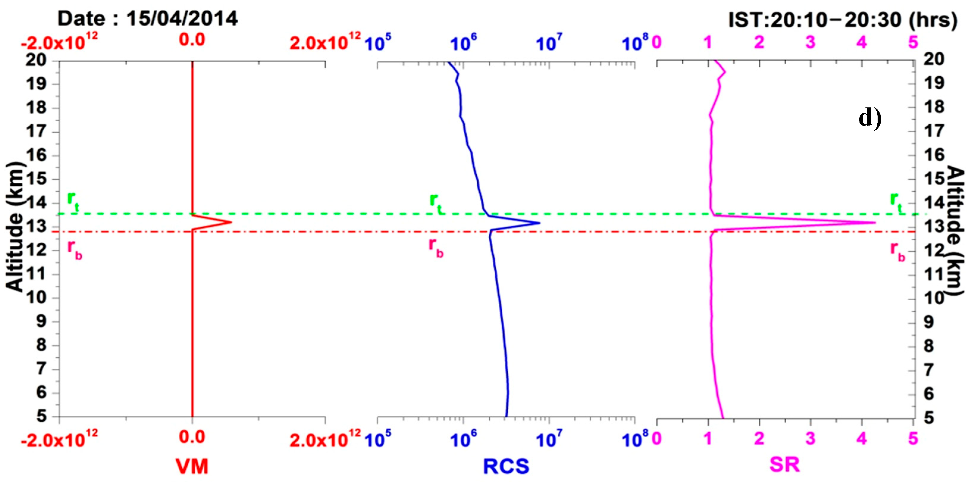
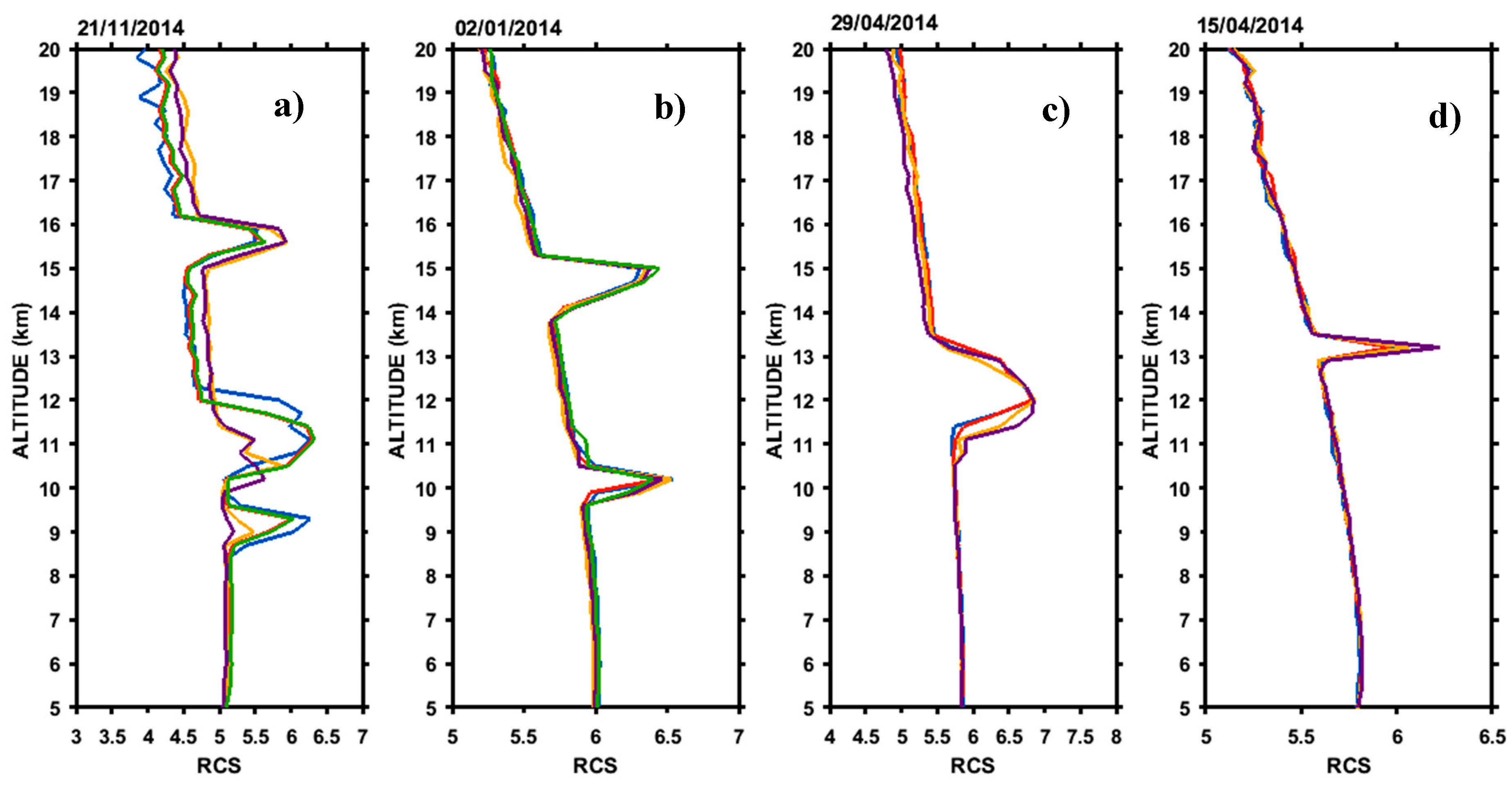
Figure 2 illustrates the VM output for the determination of the geometrical properties of cirrus clouds which were observed on 21/11/2014, 02/01/2014, 29/04/2014, and 15/04/2014 at 23:09–23:29 h, 22:38–22:58 h, 21:02–21:18 h, and 20:10–20:30 h (IST), respectively. This method is also able to detect the multiple, thick, and thin cirrus cloud layers.
Figure 2a–d represent the vertical output profiles of VM which correspond to the vertical profiles of RCS and SR in the presence of multiple, dual, thick, and thin cirrus cloud layers. In all the cases, VM output profiles are compared with both RCS and SR profiles, which showed good agreement with the most possible accurate values. The base and top altitudes of cirrus clouds detected using VM, RCS, and SR is shown in pink-red (dash-dotted) and green (dash) lines. The three layers of the cirrus clouds were observed on 21/11/2014 at the altitudes of 9 km, 11 km, and 15 km with their CiMH’s of 9.15 km, 11.1 km, and 15.6 km, respectively. The dual layer cirrus clouds were observed on 02/01/2014 at the altitudes of 10 km and 14 km with their CiMH’s of 10.05 km and 14.55 km, respectively. The thick layer cirrus cloud (whose thickness was about 2.4 km with an optical depth of 0.383) was observed on 29/04/2014 at an altitude of 11 km with a CiMH of 12 km, and the thin layer cirrus cloud (whose thickness is about 0.6 km, i.e., two range bins with an optical depth of 0.069) was observed on 15/04/2014 at an altitude of 13 km with CiMH 13.2 km. Typical idealized plots of various logarithmic RCS profiles corresponding to VCM output profiles are represented in
Figure 3a–d. The details of the geometrical and optical characteristics of the cirrus clouds which include cloud base, middle, and top heights, geometrical thickness, and tropopause height (which is the height at which the temperature in the radiosonde measurement is minimum) [
21,
22], as well as the optical depth during the observation days measured by the VM output are presented in
Table 1.
4.2. Temporal Variations of Cirrus Clouds
The operation of the lidar was on a continuous basis and observations were made for 154 nights in the year 2014 and 128 nights in the year 2015. During this observational period, cirrus clouds were detected only for 99 nights (64%) in 2014 and 46 nights (35%) in 2015.
To understand the time variation and structure of the cirrus clouds, prominent seasonal days are preferred during the period of observation. Pseudo-color plots of
Figure 4a–d and
Figure 5a–d represent the temporal variations of typical cirrus cloud scattering ratio profiles observed in four different seasons of the selected four different nights for the years 2014 and 2015, respectively. The single, dual, and multiple layers of cirrus clouds as well as the thick and thin cirrus clouds have also been observed at various heights during these prominent seasons from the lidar scattering ratio profiles.
4.3. Geometrical Properties of Cirrus Clouds Over Gadanki
4.3.1. Cirrus Percentage Occurrence
It is essential to know the effect of cirrus clouds and their occurrence over the tropical regions. The occurrence/frequency (in percentage) of cirrus clouds with respect to the observed cirrus heights (km) is calculated. In general, the percentage of occurrence of cirrus clouds is obtained by taking the ratio of occurrence of cirrus clouds in hours to the total number of hours of the lidar operation which is multiplied with a hundred. In the same manner, the percentage occurrence of the cirrus geometrical properties like cirrus base, middle, and top heights, and thickness are also calculated. The percentage of cirrus occurrence was calculated primarily at heights from 8 km to almost 20 km.
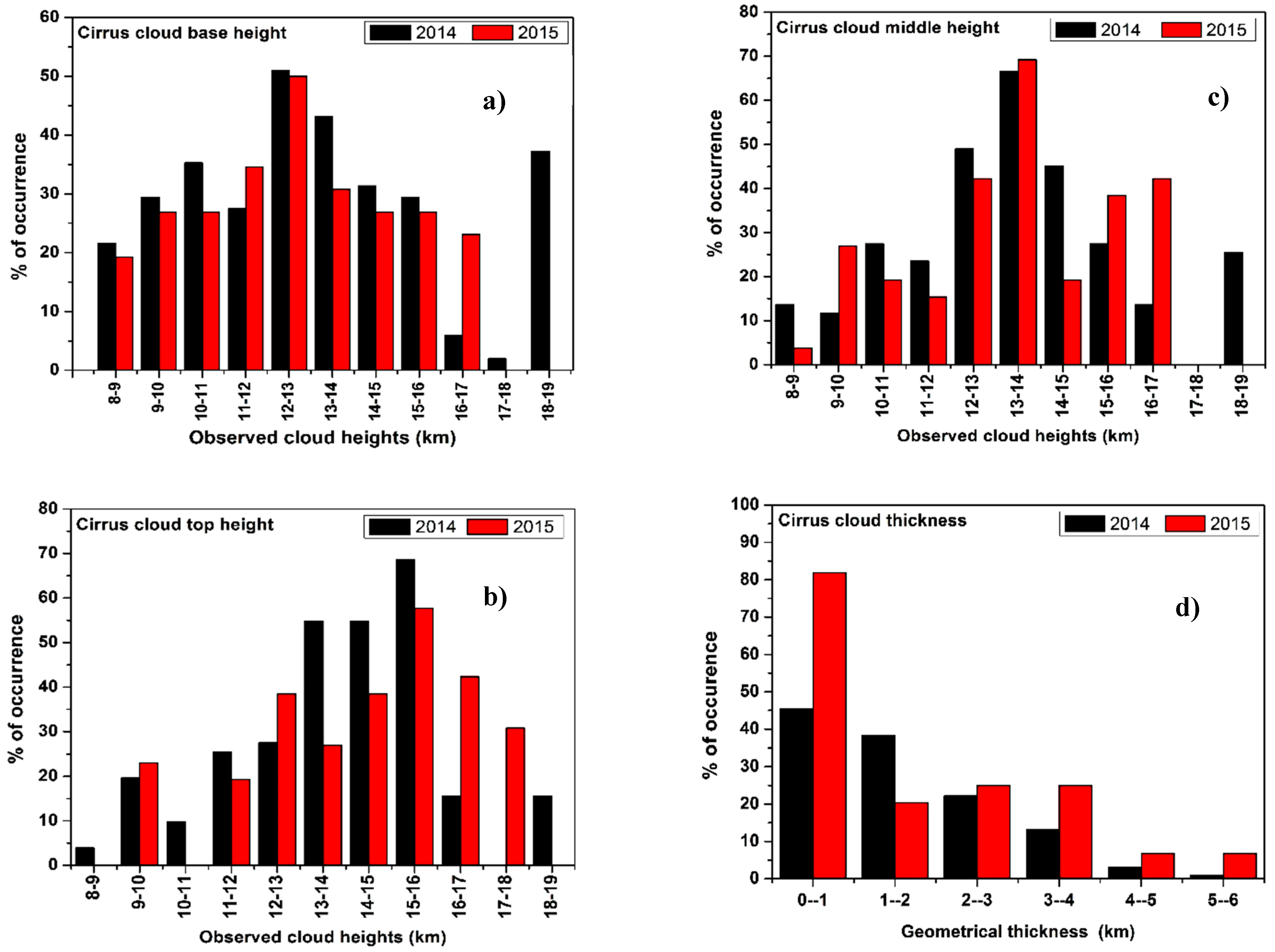
Figure 6a–d shows the variations of percentage occurrence of cirrus clouds with respect to the observed cirrus cloud heights over Gadanki during the period from January 2014 to December 2015. During this period the percentage occurrence of cirrus base heights among all layers was distributed between 8.4 km to 18.6 km. The base heights of cirrus clouds (
Figure 6a) are in between 12 km and 13 km and are distributed to a maximum of 50.9% and 50%, respectively. This is in good agreement with 12 km and 14 km [
23]. The most possible occurrence of top heights of cirrus clouds (
Figure 6b) observed at Gadanki lie between 15 km and 16 km which are near the tropopause. The top heights are distributed with a maximum occurrence of about 68.6% and 57.6%, respectively during the period of observation. This is in good agreement with the 16 km range [
24] and 13–15 km range [
25]. The maximum occurrence of the middle heights of cirrus clouds is around 66.6% (2014) and 69.23% (2015) in the height range of 13–14 km as shown in
Figure 6c. Generally, the middle height of cirrus occurs close to the tropopause. Interestingly, in the height range of 17–18 km, there are no occurrences of top heights for the year 2014, base heights for the year 2015, and no middle heights for both the years. Owing to the limitations in data observations during the year 2015, no cirrus top heights were found in the height ranges of 8–9 km, 10–11 km, and 18–19 km.
Table 2 gives the statistical details of the geometrical characteristics of cirrus clouds obtained from the lidar dataset over Gadanki for the years 2014 and 2015.
The variation of percentage of occurrence of the cirrus clouds over the geometrical thickness for the years 2014 and 2015 is shown in
Figure 6d. It is observed that the thickness of cirrus clouds vary between 0.7 km and 5.7 km. The geometrical thickness of the cirrus clouds formed seems to be thin, which is observed for all layered clouds in the height range of 0.3 km to 1 km. It can be seen that the maximum occurrence of about 45% and 81% (for 2014 and 2015) of the total cirrus clouds formed are thin cirrus with a thickness of less than 1 km. Around 38.3% and 20.4% of the cirrus clouds formed during 2014 and 2015 are also thin cirrus clouds having a thickness of less than 2 km. It is found that a large number of cirrus clouds appeared to be thin over the thickness range of 0–1 km and 1–2 km. The occurrence of cirrus clouds is found to be minimum in the geometrical thickness range of 5–6 km with a value of 1.1 % (2014) and 6.8 % (2015). The presence of thin cirrus clouds having a thickness range of 0–1 km and 1–2 km could be seen below the tropopause and they mostly occurred in the height regions around 12 km, and above 15 km.
4.3.2. Monthly and Seasonal Variations of Cirrus
The monthly mean and seasonal variations of the tropical geometrical properties of cirrus clouds with respect to height were observed for all the layers of the cirrus clouds and persisted during the nighttime.
Figure 7 shows the bar charts of the total hours of the lidar and the total hours of cirrus cloud observations for every month over the Gadanki region. The asterisk (*) symbol in
Figure 7 indicates that no lidar observations were made which may be unavoidable under non-operational circumstances. The symbol (#) denotes the occurrence of cirrus clouds even when the lidar observations were made. The lidar operation depends predominantly on the weather conditions, and the measurements were not continuous for all the months, and hence it is appropriate to express the statistical data in terms of monthly variations.
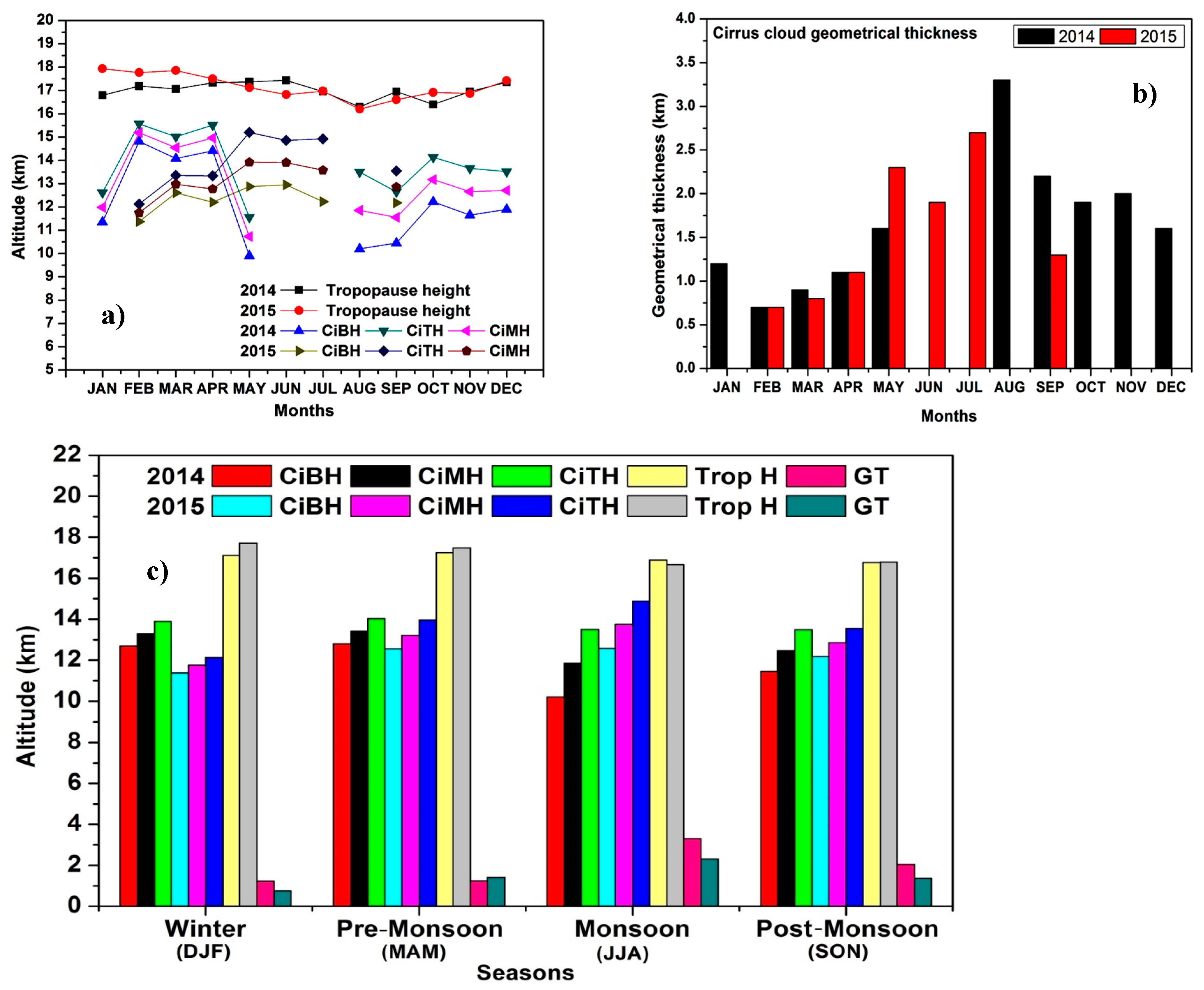
The two years of NARL lidar datasets (2014 and 2015) obtained to study the monthly and seasonal variability of cirrus clouds near Gadanki during the night time are shown in
Figure 8a–c, respectively. The monthly variation is also studied from the seasonality of the cirrus clouds.
Figure 8a,b shows the monthly variations of base, top, and middle height, Tropopause Height (Trop H) and Geometrical Thickness (GT) of cirrus clouds. It can be seen from
Figure 8a that the cirrus base and top heights had high values in the months of February, April, and October during 2014 and it was highest during February 2014. The cloud base and top had the lowest value during May in 2014. For the year 2015, the base height of cirrus clouds had maximum values during March, May, and June and minimum values during Feb 2015. The observed top heights of cirrus clouds had high values during May, June, and July 2015. In 2015, the highest value of the cirrus top occurred during May and the lowest value during February. During the years 2014 and 2015, no cirrus cloud tops could be seen close to the tropopause, but they were seen near it. It was observed that the cirrus clouds are present at a lower height of around 9.6 km during the month of May 2014.
The four prominent seasons of the Gadanki region are pre-monsoon—(MAM), monsoon—(JJA), post-monsoon—(SON), and winter—(DJF). With the limited lidar data, it was difficult to study the seasonal behavior but a general tendency could be analyzed by observing the data. The seasonal variations of the geometrical properties of the cirrus clouds for the year 2014 and 2015 are illustrated in the
Figure 8c. It shows that the base and top heights of cirrus cloud had the highest values during the pre-monsoon season and the lowest during monsoon seasons for the year 2014. In 2015, the highest and lowest values occurred during the monsoon season and winter season. The geometrical thickness with a maximum value of 3.3 km and minimum value of 1.2 km was observed during the monsoon and winter seasons during 2014 and 2015, and had the highest value of about 2.3 km and 0.7 km for the above seasons, respectively. It can be concluded that for both the years, cirrus clouds were thin in the winter season and thick in the monsoon season. The tropopause height was high in the year 2014 of about 17.2 km in the pre-monsoon season and of low value of about 16.7 km in the post-monsoon season. In 2015, the highest value for the tropopause height was about 17.7 km during the winter season and had a lowest value of 16.6 km in the monsoon season.
4.4. Optical Characteristics of Cirrus Clouds Over Gadanki
4.4.1. Optical Depth
The experimental variability in optical depth,
mainly depends on the composition and geometrical thickness of the cloud and is a key parameter in the computation of the radiative transfer and hence an attempt is made to determine its values. In this study, the range of the optical depth of the cirrus cloud was found to be 0.09–0.33 for the year 2014, and for the year 2015 it was between 0.15–0.31. It is observed from
Figure 9a,b that
of cirrus clouds shows a similar dependent tendency with the geometrical thickness for the years 2014 and 2015. As mentioned earlier, due to difficulties in the operation of the instrument under terrible weather conditions, the values show zero in
Figure 9a,b. The measured cirrus cloud
for the years 2014 and 2015 are in between 0.01 and 1.0.
Previous lidar observations [
2,
26] report on the statistics of the optical depth of cirrus clouds. The cirrus clouds are classified based on their optical depths;
< 0.03 is classified as Sub-Visual Cirrus (SVC), 0.03 <
< 0.3 as optically Thin Cirrus (TC), and
> 0.3 as optically thick cirrus, Dense Cirrus (DC), or opaque cirrus clouds. [
12] proposed the threshold value of 0.03 in order to divide the cirrus clouds from visible (thick and thin) to sub-visual and the same approach is followed in the present study. For further analysis on the distribution of the optical depth, a bar chart diagram is presented in
Figure 9c. It is found that for the year 2014, 14.8% of cirrus clouds are sub-visual in nature, 75.2% of clouds are TC, and 9.9% of clouds are DC. For the year 2015, it was found that 71.2% clouds were TC and 28.7% were DC. No sub-visual cirrus clouds were found in 2015. Our results show (during the years 2014 and 2015), that more than 70% of the cirrus clouds were optically thin (i.e., 0.03 <
< 0.3). It can also be observed from
Figure 9c that the cirrus clouds are highly thin and a little thick during the year 2014 and 2015.
Figure 9d presents the monthly variation of the depolarization ratio of cirrus clouds for the years 2014 and 2015. During 2014, the depolarization ratio had relatively higher values in the months of January, March, and September. The highest value was observed in the month of March (pre-monsoon season). During 2015, DR had higher values in the months of February, June, and July and the highest value was observed during July (monsoon season). It was observed that the pre-monsoon season had lower values of DR during May 2014 and March 2015.
4.4.2. Depolarization Ratio
Generally, spherical water droplets cause zero depolarization, whereas non-spherical ice clouds produce depolarization. Thus, the depolarization ratio
is a measure of the non-sphericity of the cloud particles. In the tropics, cirrus clouds are mostly composed of non-spherical ice crystals which cause significant depolarization. The values of the depolarization ratios (DR) vary widely due to the composition of the cloud which results in nucleation processes. The DR values associated with different shapes of ice crystals exist within the cirrus cloud around 12 km [
27]. High altitude cirrus clouds with larger DR values of > 0.3, moderate values of DR in the order of 0.3, and lower DR values of < 0.3 indicate the presence of different compositions of ice crystals present in cirrus clouds [
28].
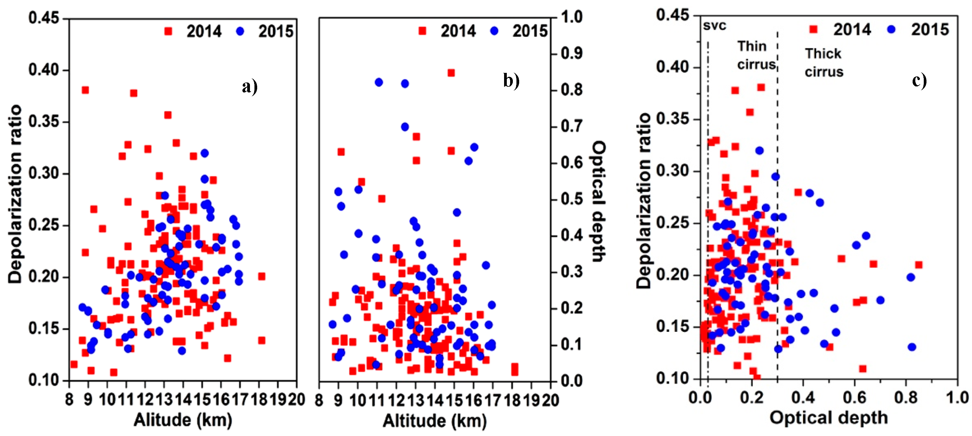
Scatter plots (
Figure 10a–c) show the height variation of the depolarization ratio and optical depth for the years 2014 and 2015. In
Figure 10a, a slight abnormality is observed in the profiles of the depolarization ratio for the year 2015 compared to that of 2014. Less depolarization ratio was observed at the middle cloud during 2015 compared to that of 2014. For the years 2014 and 2015, an increasing tendency was observed for DR values in the heights ranging from 11 km to 15 km with values ranging from 0.15 to 0.25. In between 16–18 km, the depolarization ratio was less than 0.25 (2014) and 0.32 (2015). The most widespread region of the depolarization ratio values of cirrus cloud was found between 0.2 and 0.25 for the year 2014 and between 0.15 and 0.2 (2015). The moderate DR values of cirrus clouds were observed in the height range from 12 km to 16 km for both the years signifying the presence of thin plates or horizontally oriented ice crystals.
Figure 10b shows a slight anomaly in the scatter plot of optical depth profiles for 2015 compared to that of the observations made in 2014. In 2014, a variation in optical depth was observed with values ranging from 0.502 to 0.849 in the height regions of 9 km and 15 km and in 2015, it ranged from 0.514 to 0.822 in the height regions of 9 km and 11 km, respectively.
Figure 10c depicts the classification of cirrus clouds based on the variation of optical depths against the depolarization ratio for 2014 and 2015. A correlation between the optical depth and the depolarization ratio is also observed and the correlation was negative (−0.0303) during 2014 and positive (0.1311) during 2015. In the year 2014, DR values of sub-visual cirrus clouds, ranging from 0.15 to 0.25, were observed in the optical depth range from 0.016 to 0.029. DR values of thin cirrus clouds ranging from 0.13 to 0.37 were observed with optical depths ranging from 0.031 to 0.297. In case of the thick cirrus clouds, the DR values ranging from 0.12 to 0.36 were observed with the moderate optical depth values ranging from 0.304 to 0.849. During 2015, it is observed that thin cirrus clouds had DR values ranging from 0.13 to 0.35 with optical depths ranging from 0.046 to 0.292, and thick cirrus DR value ranges from 0.12 to 0.28 had optical depths varying between 0.303 and 0.822, respectively. Depending on the height and optical depth, a variation in DR values was found for sub-visual cirrus, thin cirrus, and thick cirrus clouds during the period of observation.
5. Conclusions
In the present work the geometrical properties of tropical cirrus clouds are observed and analyzed using the data set of Mie lidar for the year 2014 and 2015 over Gadanki, India. The variance method, a statistical approach, was applied to find the geometrical characteristics of the lidar observed cirrus clouds. Output of the variance profile was compared with the profiles of the lidar-range corrected signal and scattering ratio. A maximum occurrence of cirrus clouds with a geometrical thickness of 45% (2014) and 81% (2015) was observed over this region. Most of the cirrus clouds were found to be thin clouds having a thickness ranging between 0.5 km and 2 km. The cloud thickness ranging from 0.7 to 5.2 km with a mean thickness of 1.3 ± 1.1 km and 1.7 ± 1.4 km respectively was observed during that period. From the measured optical depth values, the cirrus clouds were categorized as sub-visual cirrus (14.8% for 2014), thin cirrus (75.2% for 2014 and 71.2% for 2015), and thick cirrus (9.9% for 2014 and 28.7% for 2015). During the year 2015, no sub-visual ( < 0.03) cirrus clouds were found. On average, around 70% of the observed cirrus clouds were optically thin clouds (0.03 < < 0.3). The height distributions of the optical depth and depolarization ratio were studied and the relationship on the dependence of the optical depth with respect to the depolarization ratio is also discussed. A negative correlation was observed between the depolarization ratio and optical depth during the year 2014 and positive correlation for the year 2015. Thus, a statistical variation of the tropical characteristics of cirrus clouds is presented for the period of observation.
The obtained results will be highly useful for incorporating the characteristics of cirrus clouds into the atmospheric circulation model. Due to certain nonoperational circumstances, and also due to bad weather conditions, the data could not be obtained continuously and hence there were missing data during the period of observation. A general tendency is shown in this study by observing the seasonal and monthly behavior with the limited available data. Usually this method is applied to determine the height of atmospheric boundary layer below 5 km. Since the present study has given positive results for the cloud layers from 7 km to 20 km range, this method can be widely applied to determine the properties of various clouds from the ground to the 20 km range.


