Article

Outdoor Air Temperature Measurement: A Semi-Empirical Model to Characterize Shelter Performance

1
Centre National de la Recherche Scientifique, UMR 6285, 56000 Vannes, France
2
Centre National de la Recherche Scientifique, IRSTV, FR 2488, 44321 Nantes, France
3
École Centrale Nantes, Centre National de la Recherche Scientifique, LHEEA, UMR 6598, 44321 Nantes, France
4
Soleneos, 49750 Val du Layon, France
5
Cerema Ouest, 44200 Nantes, France
6
Centre National de la Recherche Scientifique, UMR 6183, 44321 Nantes, France
*
Author to whom correspondence should be addressed.
Climate 2019, 7(2), 26; https://doi.org/10.3390/cli7020026
Submission received: 29 November 2018 / Revised: 10 January 2019 / Accepted: 22 January 2019 / Published: 1 February 2019

Abstract

:
Shelters used to protect air temperature sensors from solar radiation induce a measurement error. This work presents a semi-empirical model based on meteorological variables to evaluate this error. The model equation is based on the analytical solution of a simplified energy balance performed on a naturally ventilated shelter. Two main physical error causes are identified from this equation: one is due to the shelter response time and the other is due to its solar radiation sensitivity. A shelter intercomparison measurement campaign performed by the World Meteorological Organization (WMO) is used to perform a non-linear regression of the model coefficients. The regression coefficient values obtained for each shelter are found to be consistent with their expected physical behavior. They are then used to simply classify shelters according to their response time and radiation sensitivity characteristics. Finally, the ability of the model to estimate the temperature error within a given shelter is assessed and compared to the one of two existing models (proposed by Cheng and by Nakamura). For low-response-time shelters, our results reduce the root mean square error by about 15% (0.07 K) on average when compared with other compensation schemes.

1. Introduction

1.1. Context

Climate observation rests on the continuous monitoring of several meteorological variables. According to the World Meteorological Organization (WMO), “temperature is one of the meteorological quantities whose measurements are particularly sensitive to exposure. For climate studies in particular, temperature measurements are affected by the state of the surroundings, by vegetation, by the presence of buildings and other objects, by ground cover, by the condition of, and changes in, the design of the radiation shield or screen, and by other changes in equipment” [1]. Thus, to ensure consistency of temperature data over time, the WMO recommends that “records should be kept not only of the temperature data, but also of the circumstances in which the measurements are taken”. Such information, known as metadata, may then be used to warn a data user about the uncertainty of the temperature value over a certain time range. It may also be used to correct the data if the error attributable to this change is known.
This work is dedicated to one source of potential temperature measurement error: the shield, used to protect the sensor from long-wave and short-wave radiation. Depending on the local weather conditions and on the shield characteristics, the measured air temperature may be overestimated or underestimated. The main physical reasons for such bias are described by Jarraud [1] and by Van der Meulen [2]. They are summarized Table 1.
Van der Meulen and Brandsma [3], Barnett and Hatton [4], Erell et al. [5] showed through intercomparison campaigns that there is no shield having the most suitable characteristics for every climate condition. Thus, the intensity of the error induced by a given shield will depend on the type of climate where it is located.

1.2. Air Temperature Error Estimation

Three main methods have been proposed to study the influence of shield characteristics on the measurement error of the air temperature:
  • Data analysis of in situ and laboratory measurement campaigns,
  • Empirical modeling from observations,
  • Physical modeling.

1.2.1. Data Analysis of In Situ and Laboratory Measurement Campaigns

Lin et al. [6] showed that for a homogeneous outside wind speed, the inner shield airflow velocity is 2 to 4 times weaker (note that only two shields have been investigated). This factor depends on the outside wind speed intensity and varies within the shield along the vertical axis: the higher it is in the shield, the higher the wind speed. They also showed that the lamellas constituting the shield may have a high thermal inertia. For the two studied shields, when the wind speed is lower than 2 m·s 1 , the shelter structure time constant varies from 130 to 180 s depending on the lamella position (higher the lamella, longer the time constant). These values are clearly higher than the observed time constant of the sensor (a thermistor) used for this experiment (60 s) or the one recommended by Jarraud [1] (20 s for a 1 m·s 1 wind speed). The results of these researches also indicate that the temperature of the lamellas exposed to direct solar radiation may be up to 2 C higher than the temperature of the lamellas located in the shadow. This may result in a very different temperature error whether the lamellas exposed to the sun are located upwind or downwind. All these observations are useful to apprehend the complexity of the mechanisms involved in the error of the air temperature measurement, but they do not enable correction of biased datasets recorded using a given shield.

1.2.2. Empirical Modeling from Observation

Empirical models are used to estimate the bias generated by the use of a given shield using a given set of observed weather conditions. These models are based on equations relating temperature error ( ϵ T ) to meteorological variables that have been identified as affecting the error. The equation is composed of one or several terms ( X i —Equation (1)) being themselves a combination of one or several meteorological variables.
ϵ T = a 0 + i a i · X i
where
  • ϵ T is the air temperature error due to a shield at time t
  • a i is the regression coefficient attributed to the term X i
  • X i is the value of an explanatory variable
The combination of each term X i is based on observation rather than on physical equations and the weight of each term (coefficient a i ) is determined by regression using one or several measurement campaigns. Nakamura and Mahrt [7] proposed to use the following weather variables to explain the temperature error due to a given shield: wind speed (U), air temperature measured within the shield ( T s h ), downward short-wave radiation and net radiation (respectively for the day-time and night-time period—both noted R a d ).
ϵ T = a 0 + a 1 X N A K A
where
  • a 0 and a 1 are calculated using regression fitting
    X N A K A = R a d ρ C p T s h U
where
  • ρ = 1.2 kg·m 3 the mass density of the air
  • C p = 1004 J·K 1 ·kg 1 the specific heat capacity of the air
This equation has been used to model the error of one shield (Davis multiplate 7714) in a given environment from a measurement campaign where the reference temperature (supposed real outside air temperature) was measured within a mechanically ventilated shield (RM Young model 43408). Two measurement periods have been used: the first one was used to calibrate the models and the second to verify their performance. Cheng et al. [8] proposed to improve this model adding the solar angle parameter which was assumed to play a major role on the sensor overheating depending on the shield used. Thus, the X N A K A term has been transformed into a X C H E N term (Equation (4)).
X C H E N = R a d ρ C p T s h U · Θ 180
where
  • Θ the zenithal solar angle (in degree)
Cheng et al. [8] compared the performance of two commercial shields to a Stevenson screen. They used a first measurement campaign to calibrate the regression coefficient of their equation as well as the one of the Nakamura and Mahrt [7] equation. Then a second measurement campaign was performed to verify the accuracy of the prediction of each model. According to the results of this specific experiment (i.e., given screens and climate conditions), their model is more accurate than the Nakamura and Mahrt [7] one.
These empirical models are interesting to correct a dataset recorded using a given shield and within a given measurement site environment. However, it is not appropriate to correct a dataset recorded in other environment conditions because the thermal characteristics of the site (e.g., soil albedo and emissivity) or the climate variables (wind speed, temperature, radiation, or precipitation level) are very diverse within the world, thus impacting the regression coefficients of the models. It is also impossible to compare and analyze the effect of some specific shield characteristics on the temperature measurement since each term of the equations has no physical meaning.

1.2.3. Physical Modeling

To overcome these limitations, physical models can be used to better understand how the shield affects the temperature measured and to predict the error from weather conditions. Lin et al. [9] proposed to solve an energy balance containing all significant heat transfer terms known to affect a sensor located within a shelter. Two shelters have been tested in Lincoln (Nebraska, United States of America) during the clear days of an entire year. They have measured the incoming global radiation flux and the air temperature in each shelter using three thermocouples painted with a different coating (black, white, and aluminum) to determine the radiation fluxes taking place within the shelter. They also measured the ambient wind speed to determine the convection flux between the sensor and the air (they previously established a linear transfer function to relate the wind speed inside the shelter to the ambient wind speed [6]). Thus, they were able to characterize the distribution of the energy fluxes within each shelter for different wind speed and solar angle conditions. However, as only the interactions between a sensor and its shelter are modeled, and not the shelter itself, this model does not reproduce the time lag induced using a specific shelter on the temperature measurement. At the end of their study, the authors conclude that “the feasibility of correcting air temperature errors due to the radiation shield microclimate has been demonstrated” and that the next step would be to propose a generic transfer function that can be applied to any shield. They suggest that this function may contain the global radiation, the wind speed, and the ground surface albedo as explanatory variables. However, the shape of the model was not predicted, and their proposition do not take into account the error dynamic since they do not consider the thermal inertia effects.

1.3. Objective of the Study

In the present study, we propose to combine the strengths of each of the three methods presented in Section 1.2 while limiting their weaknesses. As proposed by Lin et al. [9], we base our model on a transfer function to characterize the measurement error induced by the use of a specific shelter. However, where Nakamura and Mahrt [7] or Cheng et al. [8] have based their model on an empirical approach (Equation (2)), we have decided to derived ours from a simplified heat energy balance applied to the system {shelter + sensor}. This transfer function model will be calibrated using observed shelter error under several meteorological conditions. As a result, our model is defined as a semi-empirical model. A WMO measurement campaign [10] is chosen as calibration dataset for the high variability of meteorological conditions (desert environment) and shelter types (18 different shelters are compared).
This work has three objectives:
  • To propose a transfer function that highlights the two main characteristics of a shield: radiation sensitivity and temperature response time
  • To verify the physical relevance of the proposed model using the observations
  • To evaluate the model ability to accurately estimate the shield induced temperature error.

2. Material and Methods

2.1. Proposed Shelter Physical Model

To propose a model based on an equation deriving from a simplified heat energy balance, several assumptions are made (the use of a detailed physical model would involve a numerical solving). First, the surface temperature of the entire shelter is supposed homogeneous. Second, the air inside the shelter and the sensor are considered to be in thermal equilibrium at any time, even so it is contradictory with previous findings. Erell et al. [11], de Podesta et al. [5] showed that the sensor temperature can actually be affected by the long-wave radiation emitted by the screen. The lack of ventilation may result in a difference of several tenths of a degree between the air temperature within the shelter and the shelter. The highest differences are observed for large sensors and under low wind speed. However, the priority of this analysis is to obtain an analytical solution of the shelter error based on a simplified energy balance. Without this assumption, no solution could be found. Thus, this second assumption is conserved and its impacts on the results could be further analyzed in future works. In the rest of the study, we will note T s h the temperature of the system {sensor + air contained within the shelter}.
Three heat energy balances are calculated: Equation (5) refers to the one applied to the shelter surface, Equation (6) to the air entering the shelter and Equation (7) to the system {sensor + air contained within the shelter}. Please note that the main physical characteristics of the generic naturally ventilated shelter and its interactions with the environment are shown Figure 1.
m s h C s h T ˙ S s h = A s h Q s h * A s h Q h s h
where
  • m s h the shelter weight (kg)
  • C s h the specific heat of the shelter (J·kg 1 ·K 1 )
  • T ˙ S s h the time derivative of the shelter surface temperature (K·s 1 )
  • A s h the shelter surface (m2)
  • Q s h * the shelter net global radiation density (W·m 2 )
  • Q h s h the shelter convective heat flux density (W·m 2 )
    A s e c s h U s h C v T i n s h = A s e c s h U s h C v T + k Q h A s h Q h s h
where
  • A s e c s h the surface of the vertical shelter cross-section (m2)
  • U s h the vertical averaged wind speed inside the shelter (m·s 1 )
  • C v the volume-specific heat of the air (J·m 3 ·K 1 )
  • T i n s h the temperature of the air entering within the shelter (K)
  • T the outside air temperature (K)
  • k Q h the ratio of the shelter convective heat flux density which is transported within the shelter
    ( m s e n C s e n + V s h C v ) T ˙ s h = A s e c s h U s h C v ( T i n s h T s h ) + A s e n Q s e n *
where
  • m s e n the sensor weight (kg)
  • C s e n the specific heat of the sensor (J·kg 1 ·K 1 )
  • V s h the volume of air included within the shelter (m3)
  • T ˙ s h the time derivative of the temperature of the system {sensor + air contained within the shelter} (K·s 1 )
  • A s e n the sensor surface (m2)
  • Q s e n * the sensor net global radiation density (W·m 2 )
A third assumption is made: there is no variation of the heat stored by the shelter structure. Thus, its convective heat flux is equal to its net global radiation flux (Equation (8)).
A s h Q h s h = A s h Q s h *
Equations (6)–(8) are combined to build Equation (9):
T ˙ s h + A s e c s h U s h C v m s e n C s e n + V s h C v T s h = k Q h A s h Q s h * + A s e n Q s e n * m s e n C s e n + V s h C v + A s e c s h U s h C v m s e n C s e n + V s h C v T
The error ϵ T induced by the shelter on the air temperature measurement is defined by Equation (10).
ϵ T = T s h T
According to this definition, Equation (9) becomes Equation (11).
ϵ ˙ T + A s e c s h U s h C v m s e n C s e n + V s h C v ϵ T = k Q h A s h Q s h * + A s e n Q s e n * m s e n C s e n + V s h C v T ˙
To solve this first order differential equation, all variables except ϵ T are considered as being in a steady state (i.e., constant over time) and the volume-specific and specific heat of the air are supposed constant over temperature. The solution of this equation is given Equation (12).
ϵ T ( t ) = 1 ζ 1 ( e ζ 1 U s h t 1 ) ( T ˙ U s h ζ 2 Q s h * U s h ζ 3 Q s e n * U s h ) + ϵ T ( t = 0 ) · e ζ 1 U s h t
where
  • t the time (s)
  • ζ 1 = A s e c s h C v m s e n C s e n + V s h C v (m 1 )
  • ζ 2 = k Q h A s h m s e n C s e n + V s h C v (m2·K·J 1 )
  • ζ 3 = A s e n m s e n C s e n + V s h C v (m2·K·J 1 )

2.2. Data

To compare the performances of many shelters traditionally used by the national meteorological institutes, the WMO implemented in 2009 a measurement campaign in Algeria [10]. The air temperature within 18 different types of shelters has been recorded during one year in desert conditions. Seven of them were artificially ventilated whereas the others were naturally ventilated.
Only information required for this study are presented in this section. Further detail about the experiment may be found in the WMO report [10].

2.2.1. Location

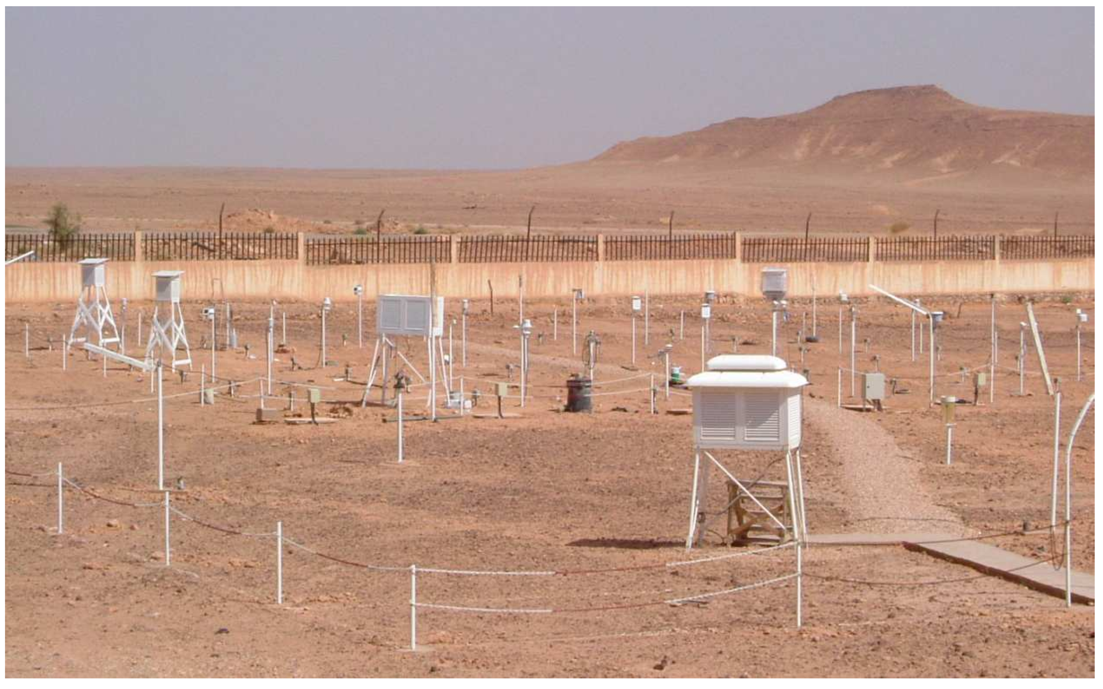
The experiment was held in the Sahara Desert at the meteorological station of Ghardaïa (32 24′ N, 03 48′ E, 468 m above the sea level). The site during the experiment is shown Figure 2.
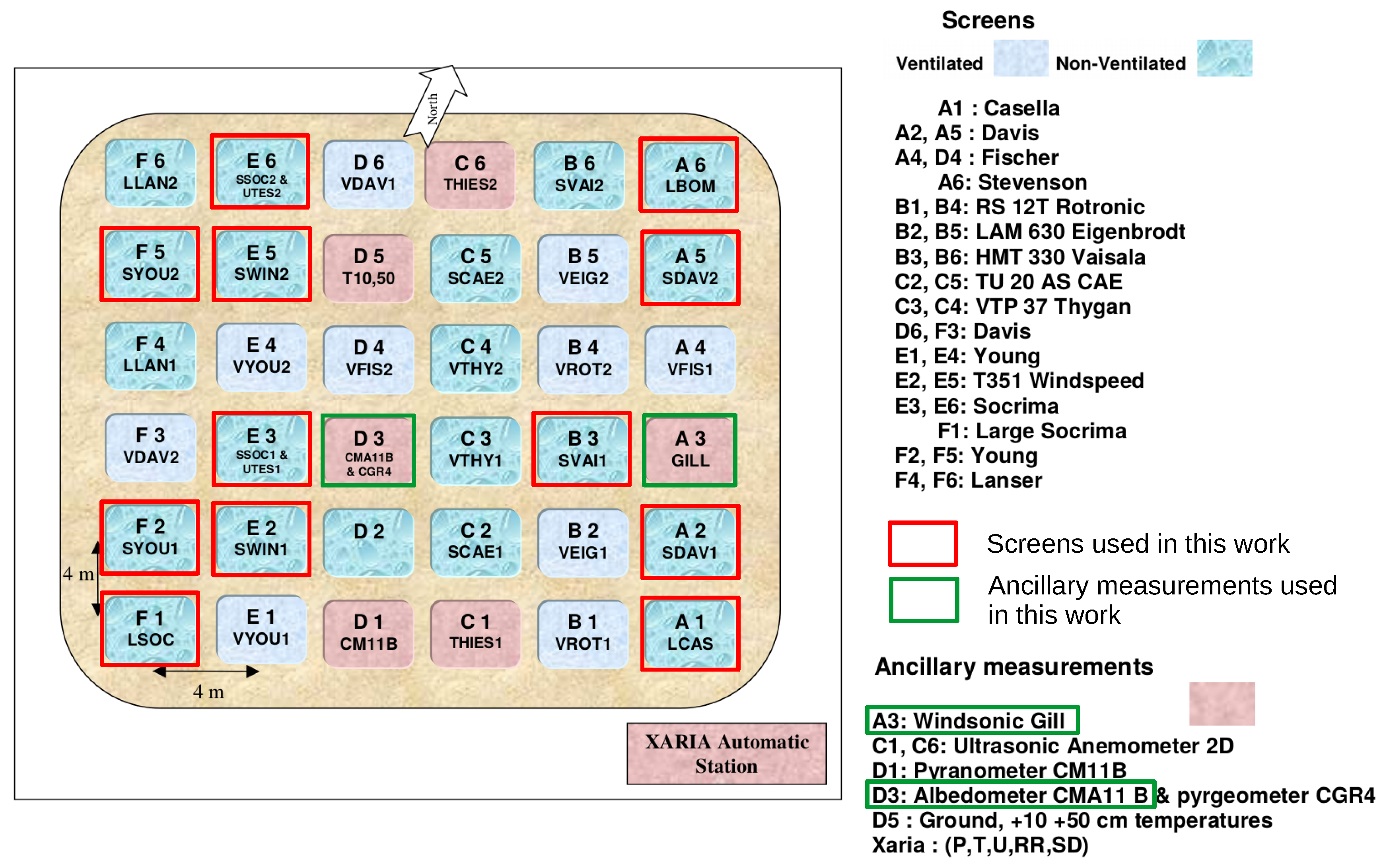
The soil of the site is flat, stony but regular. The experimental area is a rectangle containing 29 shelters (18 different types) and six ancillary sensors to characterize the meteorological conditions. The instruments are all installed at 1.5 m from the ground (except two Lanser shelters located at 1.8 m) and separated from each other by four meters according to a regular grid such as presented Figure 3. Each instrument is located near a small concrete platform where it may be electrically supplied. To avoid a potential microclimate distortion caused by a building, the experimental area is located at more than 30 m from the building of the meteorological station. Please note that the choice of this threshold may be criticized regarding new scientific results: it seems that a 50 m distance would be more appropriate [12].

2.2.2. Measurement of the Air Temperature within the Shields

The WMO intercomparison campaign is based on 29 shelters of 18 different types (cf. Table A1 of Appendix A for the complete description of all types). Certain types of shelters are defined as hybrid shelters since they are made with a ventilator located in a pipe (like most of the artificially ventilated shelters) which is itself surrounded by a naturally ventilated shelter. Hybrid and artificially ventilated shelters are excluded because Equation (13) has not been designed based on the physic of a shelter containing a ventilator. The main characteristics of the remaining naturally ventilated shelters are gathered Table 2. Further details may be found in the WMO report [10].
Each shelter protects a PT100 (platinum resistance thermometer). The temperature measurement is sampled every 10 s and then averaged at the end of every minute. This is the 1-minute data which is then used in this study. All PT100 probes (except the one located in the LBOM shelter) have been calibrated before the measurement campaign. All errors resulting from the sensor calibration were within their manufacturer uncertainty range (±0.1 C) in the temperature range 20 C to 40 C.

2.2.3. Compatibility between the Observed Meteorological Variables and the Model Terms

To use the model proposed Equation (12), we need to know the airflow within each shelter ( U s h ), the net global radiation of each shield ( Q s h * ), the net global radiation of each sensor within its shield ( Q s e n * ) and the outside air temperature heating rate ( T ˙ ). None of these variables being directly measured in the WMO measurement campaign, substitution variables are proposed Table 3. The corresponding changes in Equation (12) are also given in this Table.
U s h may be easily replaced by k U s h U since Lin et al. [6] showed that the outside wind speed and the vertical averaged horizontal wind speed within a shelter were linearly related. Concerning Q s h * , only the short-waves are considered since there is no long-wave radiation data available for the whole campaign as the installed pyrgeometer worked correctly for a limited time period (from March to May 2009). Concerning the short-wave radiations, Cheng et al. [8] showed that considering the sun height as an explanatory variable of the measurement error induced by the shelter improves the performance of the Nakamura model. Thus, the solar zenith angle is used to calculate the solar radiation flux received on a surface perpendicular to the incident solar beam (as direct and diffuse radiation are not discriminated by the measurement, we consider that the downward radiation is 100% composed by direct radiation). We also assume that the shelter albedo is identical for ascending and descending radiation and constant over time (i.e., neither affected by the dust nor by the solar radiation angle of incidence). This assumption will be further investigated Section 2.3.
We consider that Q s e n * is composed of the radiation emitted by the shelter inner surface (which mainly derived from the balance of radiation happening on its outer surface) and the radiation reaching the sensor after reflection on the shelter surface. Since the long-wave radiation is not available, Q s e n * is estimated as a ratio of the short-wave radiation received by the shelter (Table 3). The air temperature heating rate can be calculated according to the outside air temperature (Table 3). The choice to use the Davis shelter (SDAV) as a reference temperature is discussed below. Equation (12) is modified to take into account these new variables.
ϵ T ( t ) = 1 ζ 1 ( e ζ 1 U t 1 ) ( T ˙ U ζ 4 K + K s i n Θ U ) + ϵ T ( t = 0 ) · e ζ 1 U t
where ζ 1 and ζ 4 are defined by Equations (14) and (15).
ζ 1 = A s e c s h C v k U s h m s e n C s e n + V s h C v [ m 1 ]
ζ 4 = k Q h A s h ( 1 α ) + A s e n k K m s e n C s e n + V s h C v [ m 2 · K · J 1 ]
To assess the error induced by the use of a specific shelter, we need to define a reference temperature. A good shelter should respect the two following criteria [10]:
  • It should follow the outside air temperature as quickly as possible.
  • It should be the least sensible to global radiation. According to the ISO17714:2007 standard, screens “that are cooler during the day and warmer during the night are likely to be giving measurements that are closest to the truth” [13].
These criteria are consistent with the two main components of our model (response time and sensitivity to radiation). They result in the choice of SDAV shelter as reference for air temperature measurement since it is summarized as having the fastest time response and the lowest radiation error under high radiation and low wind speed [10]. The consistency between its two screens is not the best observed (90% of the values are within a ±0.3 C range against 0.2 C for the best shelter type). To avoid the potential bias induced using one of the SDAV shelters as the reference, the reference temperature is defined for every time steps as the average temperature recorded within the two SDAV shelters.
Although SDAV is described as having the best behavior in most situations, under extreme conditions of wind and radiation, it might be worse than some other shelters. In that case, those conditions should be identified and excluded from the analysis. The temperature measured under each shelter is then compared to the reference temperature under different conditions of wind and radiation. Four main findings result from this analysis:
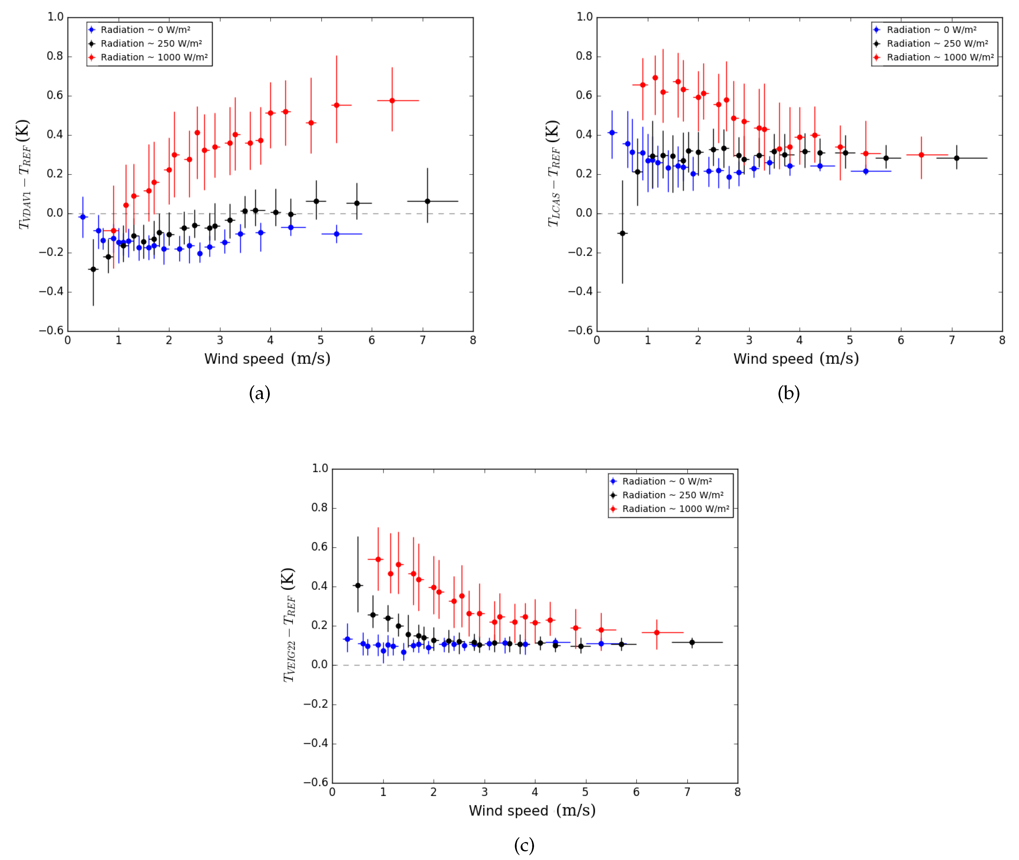
  • Under wind speed lower than 1 m·s 1 and whatever the radiation, SDAV temperature is not the highest during night-time neither the lowest during day-time (Figure 4a)
  • Under low wind speed and low solar height (about 30 for the 250 W·m 2 radiation curve), SDAV is more impacted by the radiation than some other naturally ventilated shelters (Figure 4b)
  • Artificially ventilated shelters overheat under high wind speed (Figure 4a). Please note that this phenomenon is not encountered for hybrid shelters (Figure 4c)
  • When the wind speed increases, every hybrid or naturally ventilated shelter temperature tends toward a different value whereas they were expected to tend toward SDAV temperature (Figure 4b,c).
Further details concerning the performance of each shelter are given in Table A2 of Appendix A.
Only the shelter types described in Table 2 will be modeled. SCAE shelters are excluded for orientation reasons: they have a specific face oriented southward whereas they were supposed to be oriented northward to function correctly.
Dysfunction or acquisition breaks may have happened for some sensors during the experiment. Only periods where all sensors were flagged with a good quality data were used. The flag was given by the WMO researchers from the 10-second data. The quality control was processed according to the specifications of Lacombe [14] (e.g., the instantaneous value should not vary faster than a certain threshold defined for each variable). As the sensor SVAI2 (located in one of the two SVAI shelters) add numerous breaks in the data, it has been eliminated from the analysis to maximize the sample size. Finally, the temperature within 8 shelter types (12 shelters in total) will be investigated regarding meteorological variables calculated according to data recorded by 2 ancillary sensors (Wind Sonic Gill and Albedometer CMA11B).
As SDAV does not behave better than all other shelters in such wind conditions, data recorded when U < 1 m·s 1 are excluded (which represents less than 10% of the data). The long-wave radiation being not considered, only day-time values are conserved ( Θ > 0 ). To avoid that the quotient K s i n Θ exceeds physical values, data are removed when Θ < 2 . As a result, the final sample used to evaluate our model is composed of 101,195 time steps distributed approximately equally along the year (Table 4).
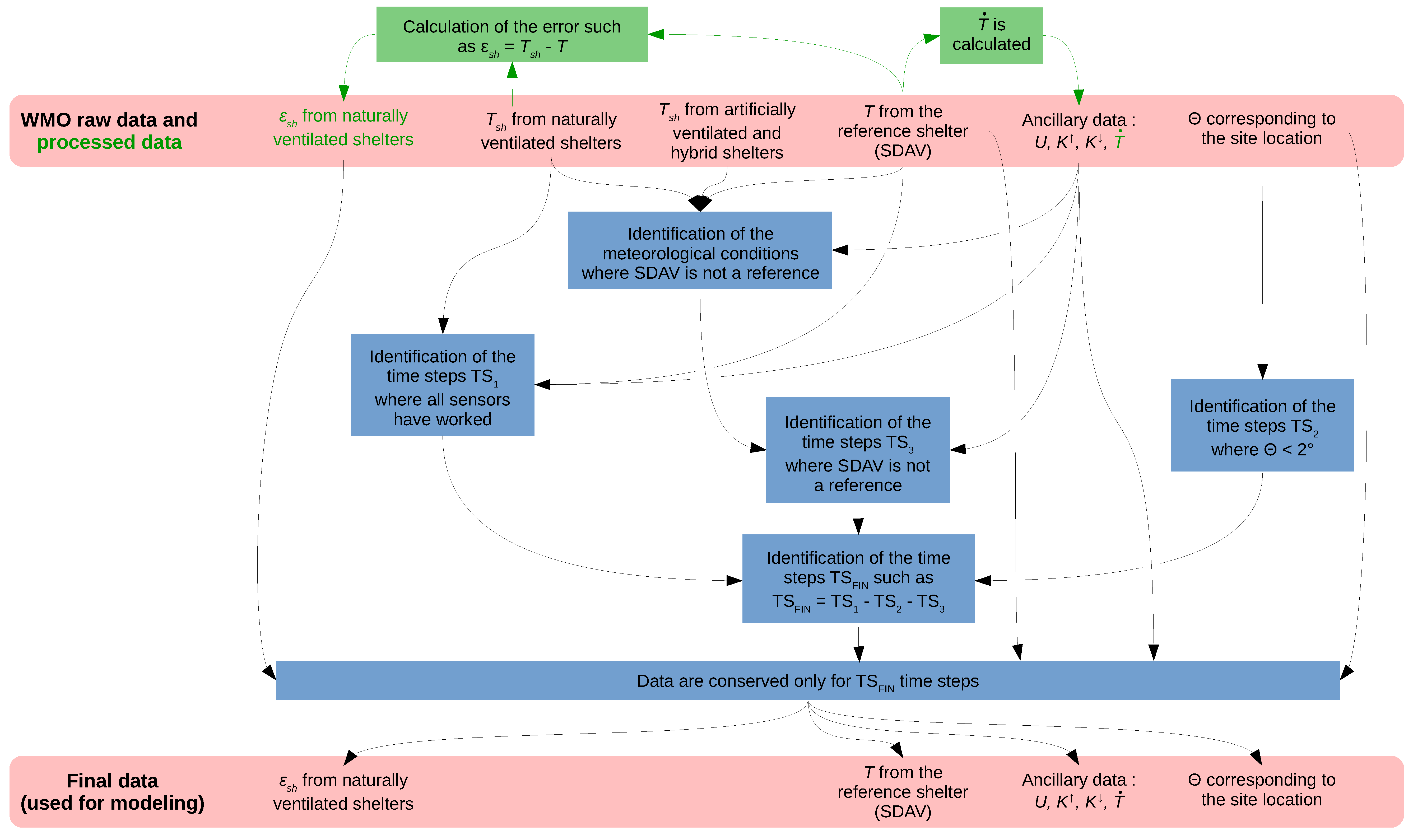
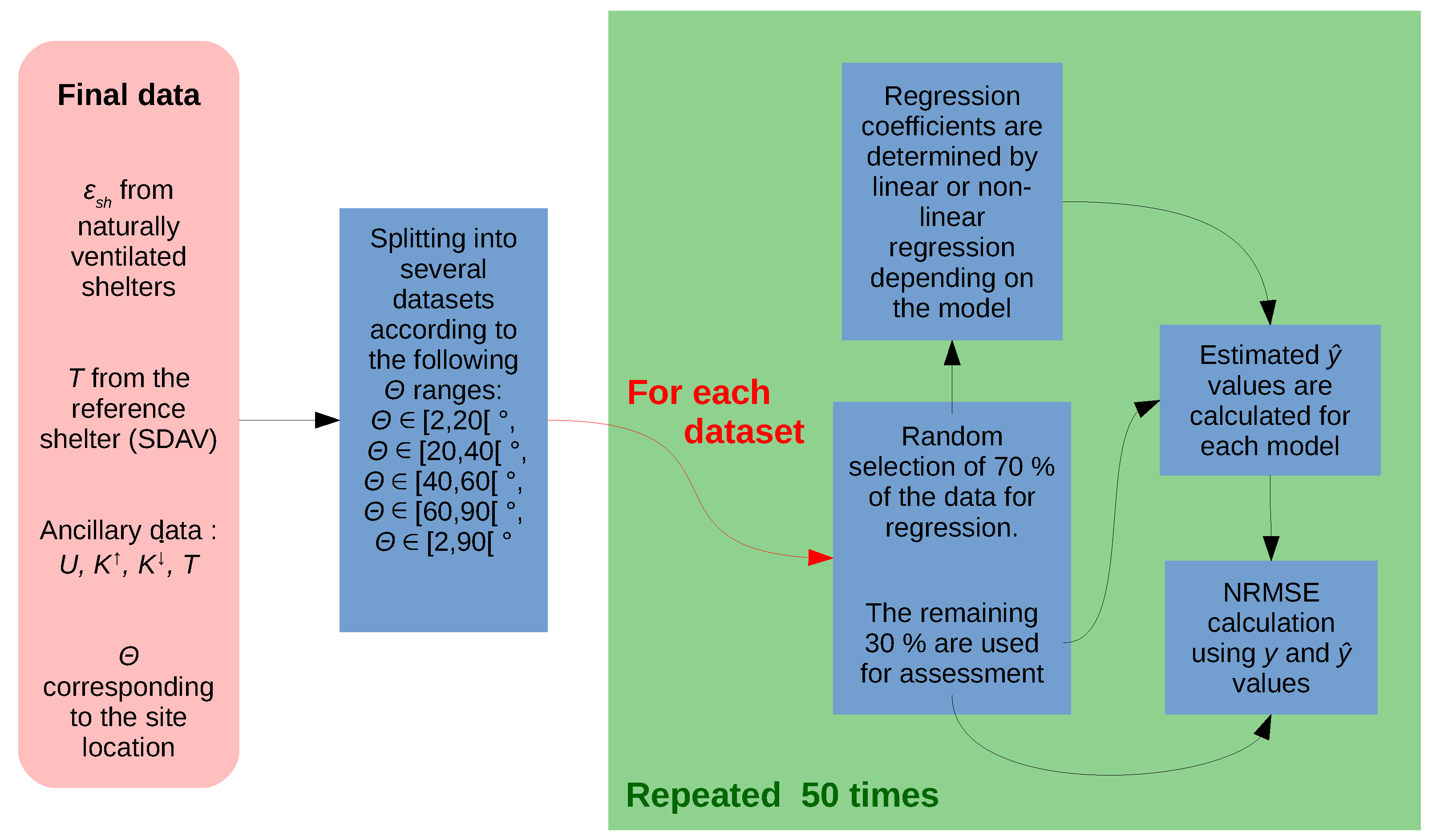
The processing chain used to select the data that are used in this work is summarized Figure 5.

2.3. Model Regression

Three models are applied to the data of each shelter to compare their respective performances: the Nakamura model, the Cheng model, and our model. Nakamura and Cheng models are solved using ordinary least square regression (The Python library called StatsModels is used for this purpose: http://www.statsmodels.org) whereas non-linear least square regression is used to solve our model (The Python library Scipy is used for this purpose: https://docs.scipy.org). The function, explanatory variables and regression coefficients associated with each model are given Table 5.
The proposed model (Equation (13)) is based on the assumption that the effective albedo of each shelter does not depend on the solar angle. To verify this assumption, the dataset used to solve the mathematical problems presented Table 5 is divided according to the following zenithal solar angle ranges: Θ [2, 20[ , Θ [20, 40[ , Θ [40, 60[ , Θ [60, 90[ , Θ [2, 90[ .
For each resulting dataset, we randomly draw 70% of the data to calculate the corresponding model regression coefficients. The remaining 30% are then used to evaluate the model performance: the observed y values are estimated ( y ^ ) using the models defined Table 5 and the calculated regression coefficients.
The proposed model is a particular case since the estimation of y at the time step t depends on the observed value of y at the previous time step t Δ t ( Δ t being the time step interval—60 s). Without reference temperature, the error at t Δ t would not be known and this model would not be applicable. Then to make our model comparable with the others, y ^ values are calculated using two different methods:
  • y is estimated according to the observed y at the previous time step: this case is an ideal case,
  • y is estimated according to the estimated y of the previous time step, itself estimated using the estimated y of the previous time step, etc. The number of previous time steps taken into account for the estimation of the error might be a critical parameter affecting the model performance. Thus, several values have been tested: 0, 5, 10, 15, 20, 25, and 30 time steps.
Finally, observed and estimated y values are compared using a normalized root mean square error (RMSE) indicator (Equation (16)).
N R M S E s h = 100 · ( 1 R M S E s h c o r R M S E s h r a w ) = 100 · ( 1 1 N i N ( y s h i y ^ s h i ) 2 1 N i N y s h i 2 )
where
  • N R M S E s h (%) the normalized RMSE of the shelter s h when its data have been corrected by a given model
  • R M S E s h c o r ( C) the RMSE of the shelter s h when its data have been corrected by a given model
  • R M S E s h r a w ( C) the RMSE of the shelter s h when its data have not been corrected (raw data)
  • N the number of time steps used for the calculation
  • y s h i the air temperature error observed within shelter s h
  • y ^ s h i the air temperature error estimated within shelter s h according to a given model
N R M S E s h is a powerful indicator regarding its interpretability capability: its value represents the percentage of the initial shelter data RMSE that can be corrected using a given model. If its value is lower than 0%, it means that the RMSE of the shelter after correction is higher than the initial RMSE (without correction).
This calibration, verification, and evaluation steps are repeated 50 times to evaluate the model sensitivity regarding the input data. The entire process used to estimate the performance of each model is summarized Figure 6.

3. Results

3.1. Physical Relevance of the Proposed Model

3.1.1. Explanatory Variables

According to Equation (13), three main terms affect the error ϵ :
  • T e r m 1 ( t ) = ζ 4 ζ 1 ( 1 e ζ 1 U t ) K + K s i n Θ U
  • T e r m 2 ( t ) = 1 ζ 1 ( e ζ 1 U t 1 ) T ˙ U
  • T e r m 3 ( t ) = ϵ T ( t Δ t ) · e ζ 1 U t
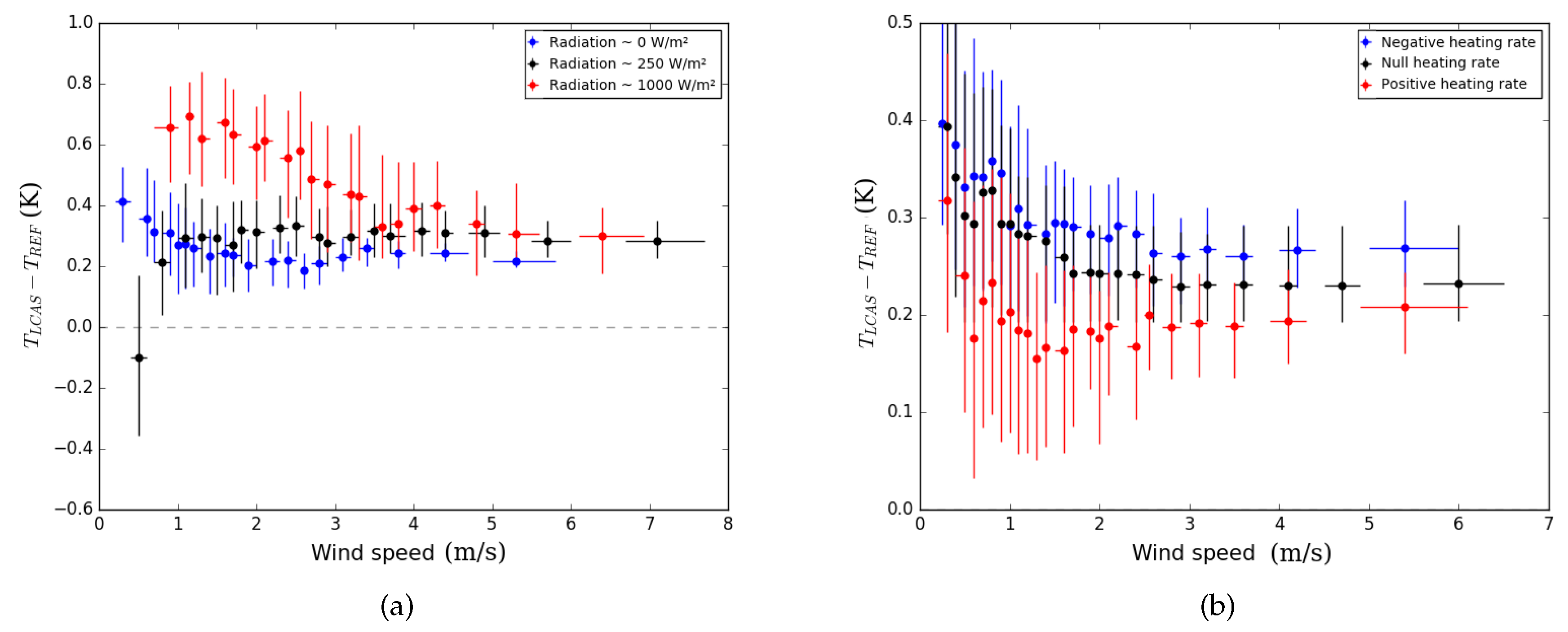
T e r m 1 and T e r m 2 should decrease identically when the wind speed increases. To analyze the influence of each term separately, low heating rate values are selected for Figure 7a and low radiation values for Figure 7b. When the wind speed increases, the error tends to a similar value for any radiation value (Figure 7a) whereas an offset remain between each T ˙ isovalue curves (Figure 7b). The observation are then consistent with the equation for T e r m 1 but slightly biased for T e r m 2 : whatever the wind speed values, an offset error dependent of the heating rate remains.
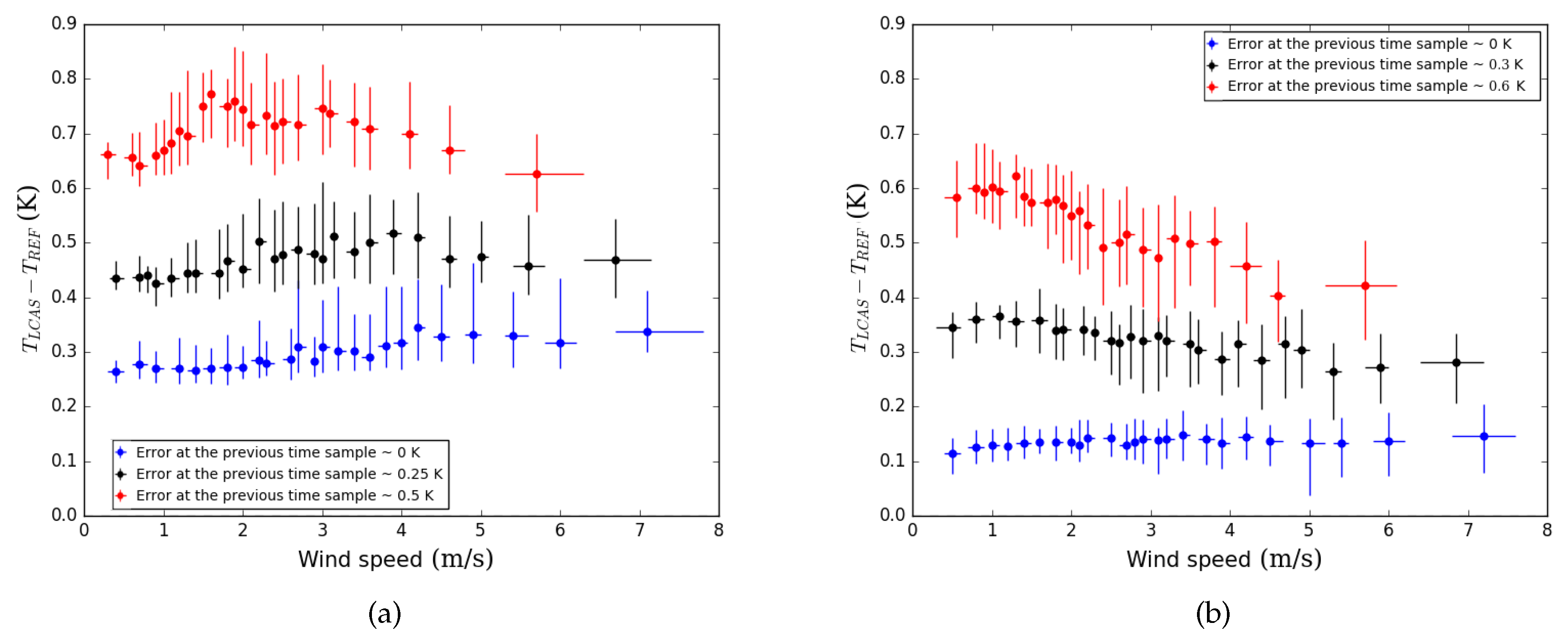
The behavior of T e r m 3 is investigated for negative (Figure 8a) and positive (Figure 8b) heating rate. In both cases when the wind speed increases, the error tends to a given value whatever the error at the previous time step (Figure 8). The consistency between observation and equation for T e r m 3 is then verified. However, as previously observed Figure 7b, the level of the offset is dictated by the heating rate value.

3.1.2. Regression Coefficients

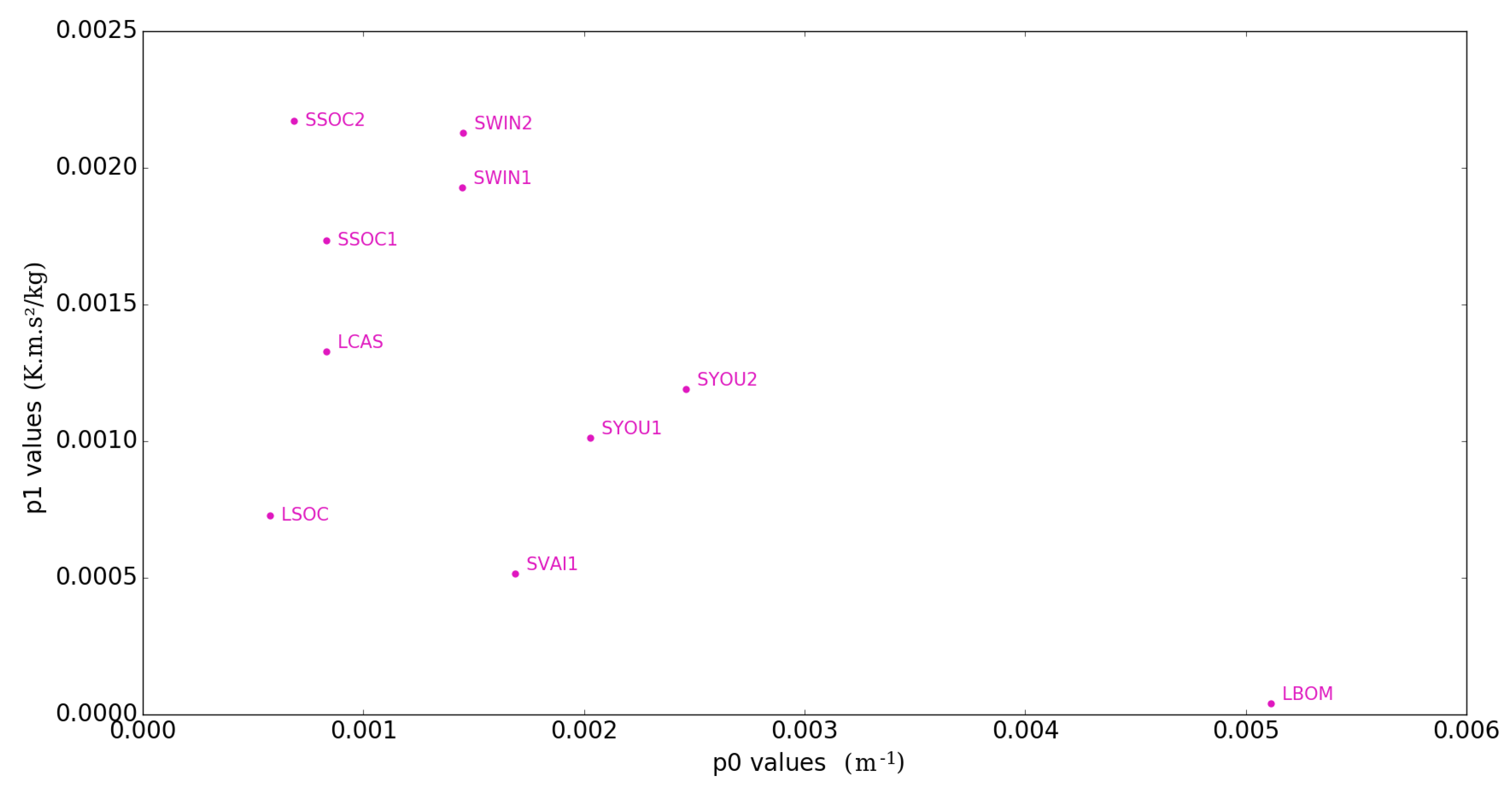
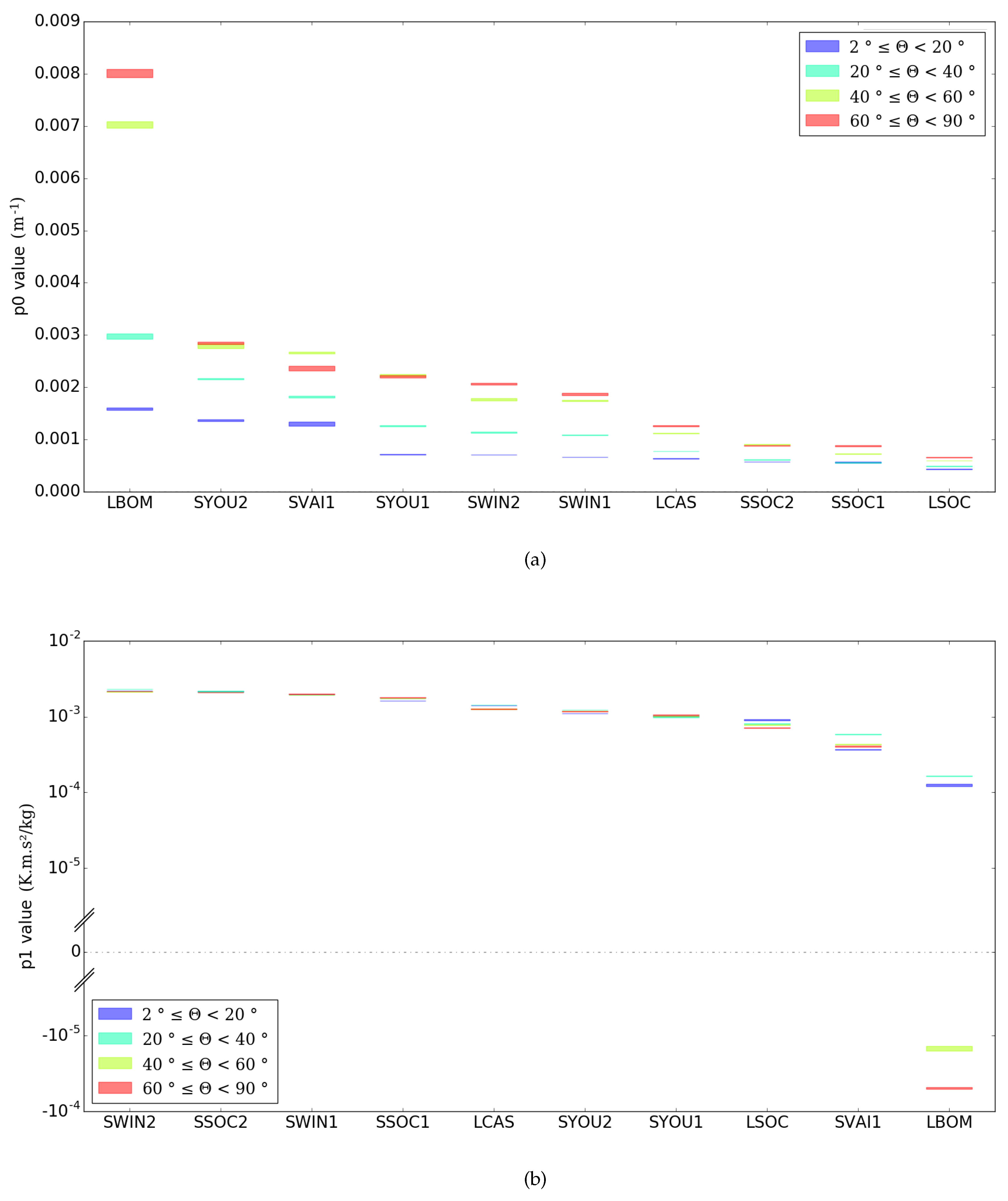
Each shelter error is not affected the same way by the terms 1, 2, and 3. This difference of behavior is explained by the variability of the ζ 1 and ζ 4 values within shelter types (i.e., the shelter characteristics). To highlight this phenomenon, p 0 and p 1 values (the regression coefficients corresponding respectively to ζ 1 and ζ 4 ) obtained for each shelter are compared (Figure 9). Please note that the entire dataset is used (2 Θ < 90 ).
According to Equation (13): lower are the p 0 values, longer is the system response time and higher are the p 1 values, higher is the shelter sensitivity to radiation. Thus, the shelters located at the bottom right on Figure 9 are the closest to the reference temperature. The furthest are logically located at the top left. In the following, these observations are analyzed in light of the temporal variations of the temperature within each shelter. For this purpose, specific events (corresponding to particular meteorological conditions) are selected.
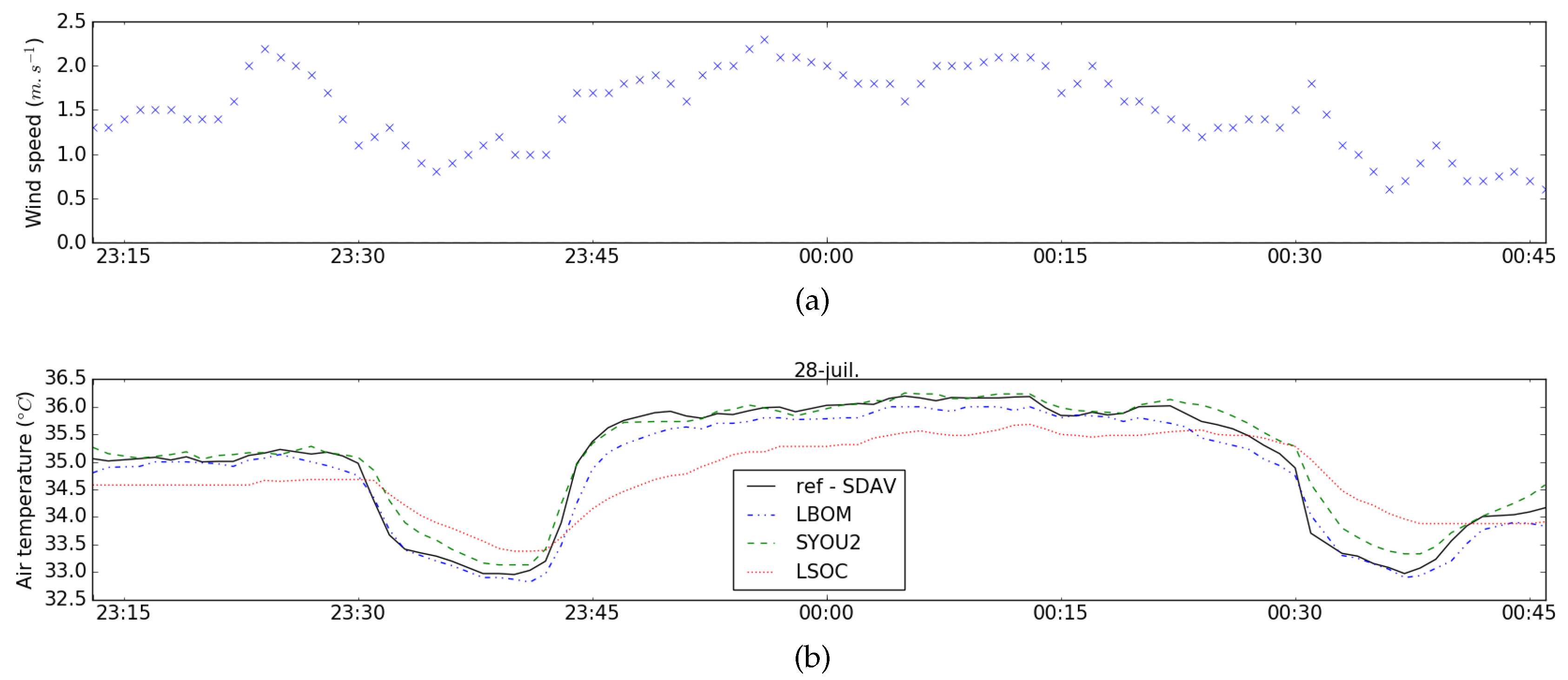
During the night of 28 July 2008, the air temperature varied quickly three times while the wind speed is almost constant (Figure 10). This period is then a very interesting sample to analyze the response time of shelters having different p 0 values. The air temperature within shelters LBOM, SYOU2 and LSOC is compared to the reference air temperature (Figure 10b). Before the fast temperature variations, SYOU2 is warmer than the reference temperature whereas LBOM and LSOC are respectively slightly and strongly colder than the reference. Then during the temperature variations, SYOU2 and LBOM are slightly lagged whereas LSOC temperature varies very slowly (the lag is much longer), which is consistent with their p 0 values observed Figure 9.
If we consider that the outside air temperature follows a unit step function around 23:45 (Figure 10), the signal temperature within each shelter should exponentially increase at different speeds depending on its time constant τ . In this case, for a first order system, the time constant level of magnitude can be estimated for each shelter. It is defined as the time the air within a shelter takes to change 63.2% of the total difference between its initial and its final temperature. According to this definition and to the Figure 10b, τ can be roughly estimated for each shelter. The time constant equation (Equation (17)) can also be identified in the exponential terms of Equation (13).
τ s h = 1 p 0 s h U
where
  • τ s h is the time constant of the shelter s h
  • p 0 s h the p 0 regression coefficient value for shelter s h
The time constant of the shelters LBOM, SYOU2 and LSOC may then be calculated for the given wind speed observed Figure 10a (about 2 m·s 1 ) using the p 0 values calculated for each shelter. Observed and calculated time constant values are compared Table 6. The level of magnitude between observed and calculated time constants is similar, which reinforces the relevance of the proposed model to explain the shelter induced error.
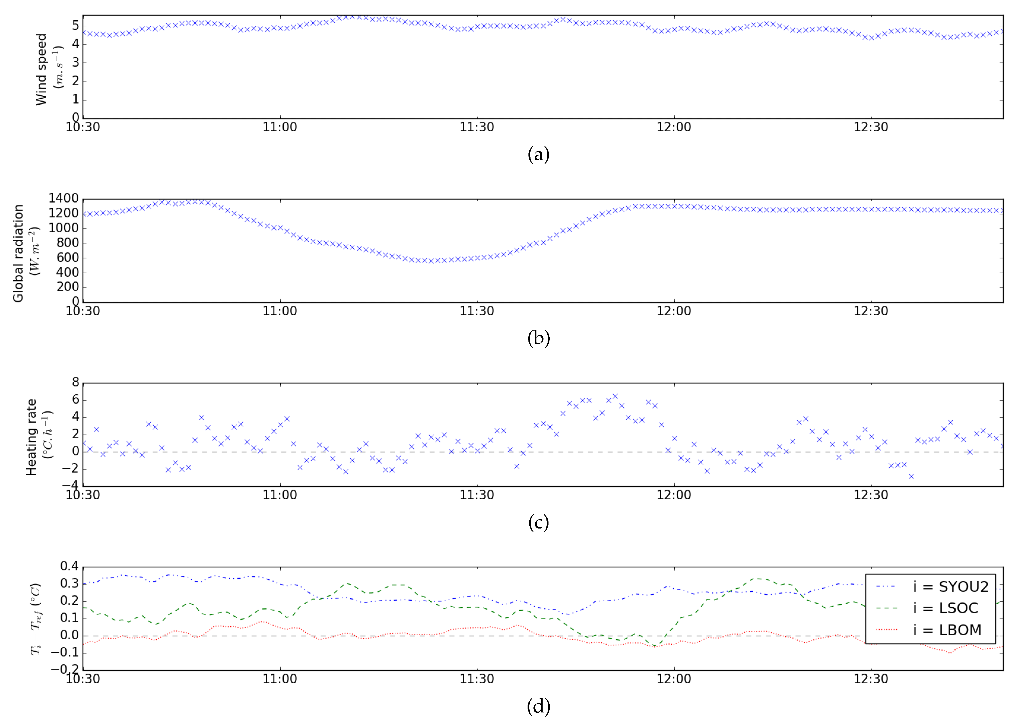
In 16 August 2008, the short-wave radiation strongly decreases for about an hour and the heating rate quickly fluctuates while the wind speed remains constant (at about 5 m·s 1 Figure 11). This period is very suitable to analyze the shelter sensitivity both to solar radiation and to heating rate values. The main variations of LSOC error are highly correlated with the heating rate: for low heating rate values, the LSOC error increases (with a small lag) while it decreases for high values (from 5 to 2 C·h 1 , the error increases of about 0.35 C). In comparison, the effect of solar radiation on LSOC error is invisible. The contrary is observed for SYOU2: it is slightly impacted by the heating rate (the error increases of about 0.03 C for a heating rate increase of about 4 C·h 1 ) while its error follows the solar radiation variations (the 800 W·m 2 global radiation decrease induces a 0.15 C decrease of the error). The last shelter (LBOM) is almost neither impacted by the heating rate nor by the radiation. All these observations are very consistent with the p 0 and p 1 values calculated for each shelter (Figure 9): the lower the p 0 values, the higher the sensitivity of the error to the heating rate values; the higher the p 1 values, the higher the sensitivity of the error to the global radiation values.

3.1.3. Sensitivity Regarding the Solar Azimuth Angle

The data has been split into several datasets, each of them corresponding to a certain solar azimuth angle range. The regression coefficients p 0 and p 1 have then been calculated for each dataset. Concerning p 0 , there is no big behavior differences among the shelters: for each of them, p 0 values are higher when Θ > 40 (Figure 12a). It means that the response time of each shelter is better when the solar radiation flux received by a horizontal surface is higher than the one received by a vertical surface. This may be explained by an increase of the air temperature difference between the top and the bottom lamellas of the shelters: it may induce a higher vertical aspiration of the air inside the shelter and thus a better ventilation rate. A second explanation could be that this range of solar height is often correlated with a high turbulence near the surface, which may also better ventilate the shelters throw vertical wind. Concerning p 1 values, they are only slightly impacted by the solar height (Figure 12b). Only LBOM values vary greatly regarding the solar height: for Θ > 40 , p 1 is negative while it is positive when Θ < 40 . This means that LBOM would be less sensible to solar radiation than SDAV when the sun is high in the sky (which is very hard to highlight analyzing temporal data).

3.2. Comparison of the Models Performance

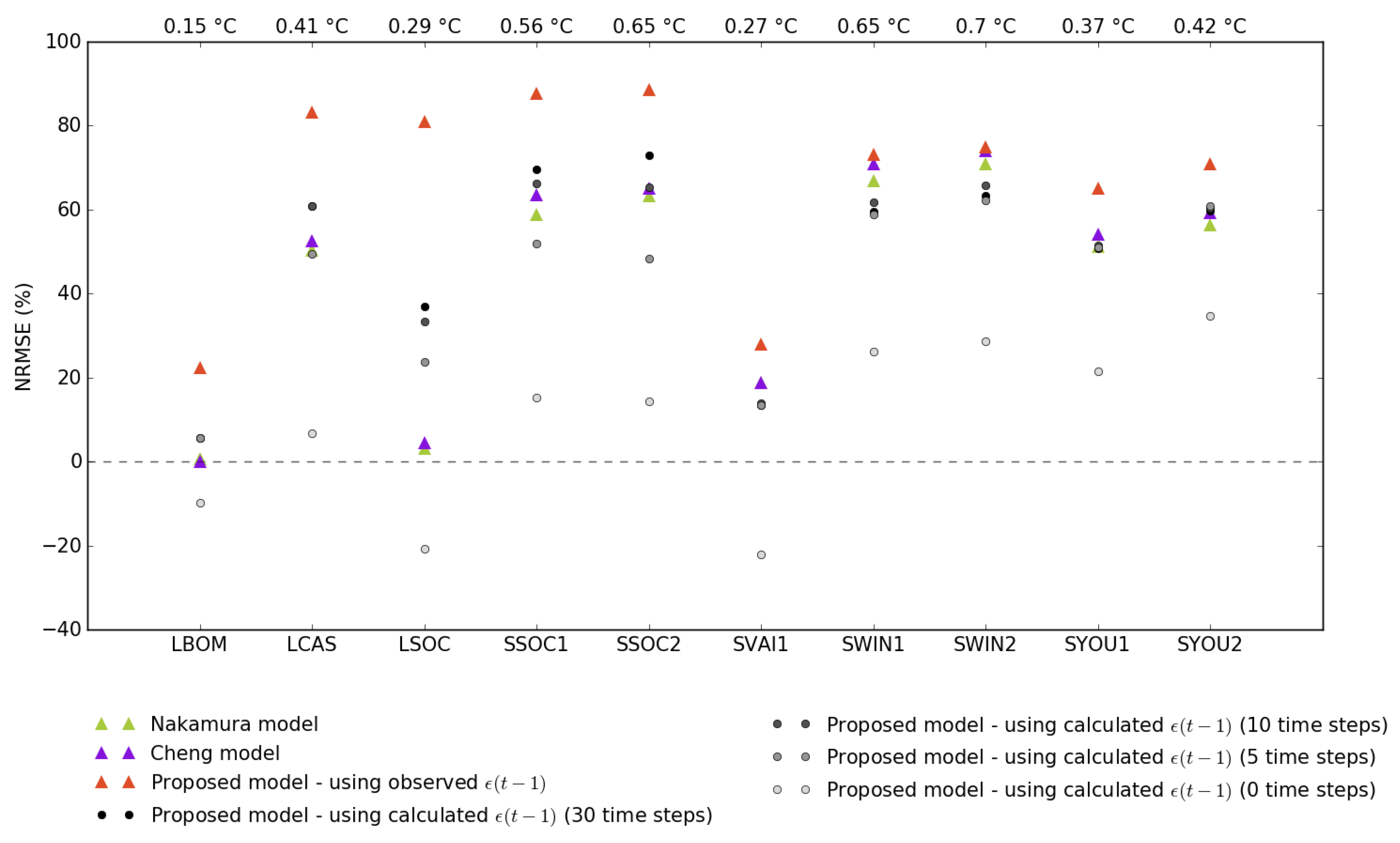
The proposed model based on the observation of the previous error works better than Cheng and Nakamura models for all shelters (Figure 13). However, this model remains theoretical since the previous observed error is never known. The proposed model based on the estimation of the previous error is then preferred for the analysis.
For LCAS, LSOC, SSOC1, and SSO2 shelters, the performance of our model strongly depends on the number of previous time steps taken into account to estimate ϵ ( t Δ t ) . During day-time, its performance still increases significantly between the one taking into account 10 time steps and the one considering 15 time steps (Figure 13). This observation is consistent with the results shown Figure 9: LCAS, LSOC, SSOC1, and SSO2 shelters are the one having the lowest p 0 values and thus the longer time response. They are then more dependent on the past weather conditions than the other shelters.
During day-time, our model works well better than the other models for 5 shelters: LCAS, LSOC, SSOC1, SSOC2 and LBOM (Figure 13). Concerning the first four shelters, it may be explained by their strong sensitivity to heating rate value (they all have low p 0 ), which our model is the only one to consider. Concerning LBOM, its sensitivity to short-wave radiations is almost nothing (cf. low p 1 value observed Figure 9). Its low error ( R M S E = 0.14 C) is then mainly due to heating rate, which is only considered in our model. The five other shelters (SVAI1, SWIN1, SWIN2, SYOU1, SYOU2) are less sensitive to heating rate values than SSOC1 or LSOC shelters and more sensitive to solar radiation than LBOM (Figure 9). Then we could expect approximately the same N R M S E value for our model than for the other models. It is true for SYOU shelters but not for the others. Concerning the SVAI shelter, Nakamura and Cheng models seem simply more appropriate whereas the better performances obtained for the SWIN shelters may be attributed to the Nakamura and Cheng model intercept. Indeed, for this shelter type, the use of the regression coefficient p 0 N ( p 0 C for Cheng) corrects between 20 and 65% of the initial observed RMSE.

4. Discussions

This work proposes a semi-empirical model to better understand, compare, and estimate the air temperature error induced by a shelter. A WMO shelter intercomparison campaign has been used to evaluate the physical relevance of this model and to evaluate its performance compared to two empirical models found in the literature.
The model regression coefficients p 0 and p 1 have been determined for each shelter. They are suitable to assess the two main components of a shelter induced error. Their values can be used to compare respectively the response time and the sensitivity to solar radiation between shelters. However, the consistency between the proposed model and the observations encountered limitations: the heating rate term seems to be less impacted by the wind speed than expected.
The values obtained for the p 0 coefficient are higher for solar azimuth angles greater than 40 . We suggest that for high solar height, a better natural ventilation of the shelters happens. This ventilation may be derived from the shelter itself (vertical winds induced by the temperature difference developed between top and bottom shelter lamellas) or from the turbulence which is often observed at this time of the day. Please note that the absence of long-wave radiation consideration may have indirectly affected the calculation of the p 0 coefficients: their dependence regarding the solar height could be attributed to a statistical fitting due to the absence of long-wave radiation in the model calibration. Please note that the values obtained for the p 1 coefficients are almost not affected by the solar height.
For low-response-time shelters, the proposed model performs better than the Nakamura and Cheng ones since Nakamura and Cheng did not take into account the shelter response-time characteristic to model the error. For most of the other shelters, we assume that the regression offset present in the Nakamura and Cheng models makes them work better for this specific dataset. This offset could have been added to our model to obtain better results. However, this would have led to two major shortcomings: first, the physical reason of this offset being not known, it could have affected the physical relevance between our model and the observations ( p 0 and p 1 would have been statistically readjusted without any physical meaning). Second, the resulting regression coefficients would have only been valid for the current WMO dataset used for the analysis.
This work raises several questions which need further investigation:
  • The response time is attributed to the shelter ventilation rate. The regression coefficient p 0 related to this phenomenon showed consistency with observation. However, this is contradictory with Lin et al. [6] observations showing that the horizontal wind speed along the central vertical axis of a shelter was sufficiently high to assume an almost instantaneous air renewal.
  • To obtain our semi-empirical model, the sensor and the air within the shelter were considered as having the same temperature at any time, which is contradictory with Erell et al. [11], de Podesta et al. [5] findings. However, the results obtained using this model are consistent with the observation.
  • The error does not tend toward zero when the wind speed increases. The offset seems to be directly dependent on the heating rate value.
  • The relationship between regression coefficients ( p 0 and p 1 ) and shelter characteristics (given by Equations (14) and (15)) have not been investigated.
  • The three models compared in this study could be calibrated using only variables commonly measured on meteorological sites (descending solar radiation, wind speed, and air temperature). The objective would then be to evaluate their respective ability to estimate the error observed at several other locations.
  • Hybrid and artificially ventilated shelters have not been modeled while it is fundamental to compare their characteristics (response time and sensitivity to radiation) to naturally ventilated shelters.
  • The long-wave radiation was not used in this study. A measurement campaign where this meteorological variable is available would be welcome to further evaluate the model and verify its performances during night-time.
  • The shelter used for the reference temperature is far from being perfect. Lanzinger and Langmack [15] proposed a calibration method in climatic chamber to access air temperature from an ultrasonic anemometer but as pointed by Richiardone et al. [16], further work should be done to obtain error-less air temperature from acoustic thermometric.

Author Contributions

Conceptualization, J.B., P.K., B.M., M.M., I.C., E.B.; methodology, J.B.; software, J.B., P.K.; validation, J.B.; formal analysis, J.B.; investigation, J.B., P.K.; resources, J.B., P.K.; data curation, J.B., P.K.; writing—original draft preparation, J.B.; writing—review and editing, P.K., B.M., M.M., I.C., E.B.; visualization, J.B.; supervision, J.B., P.K., B.M.; project administration, P.K.; funding acquisition, P.K., M.M., I.C., E.B.

Funding

This work was partly funded by the French Environment and Energy Management Agency (ADEME) and the French region ”Pays de la Loire”.

Acknowledgments

The authors wish to thank the World Meteorological Organization to freely allow the use of their climate measurement campaign data. We also would like to thank the researchers who have implemented the measurement campaign in Ghardaïa and their very detailed reporting. A special thanks to Michel Leroy for the data and documentation providing and for its availability during our project.

Conflicts of Interest

The authors declare no conflict of interest.

Abbreviations

The following abbreviations are used in this manuscript:
WMOWorld Meteorological Organization
RMSERoot Mean Square Error

Appendix A. Detailed Informations about the WMO Shelters and Their Respective Performances

Table A1. Main Informations Concerning the 29 Shelters Used during the WMO Campaign.
AcronymManufacturerTypeVentilation TypeClosest ShapeMaterialNumber of Shelters
LBOMBoMSmall Stevenson screennaturalcuboidwood1
LCASCasellaStevenson screennaturalcuboidwood1
LLANLanser hybridcuboidwood2
LSOCSocrimaLarge Stevenson screennaturalcuboidplastic1
SCAECAETU20ASnaturalcylindricduralinium2
SDAVDavisPN7714naturalcuboidplastic2
SSOCSocrimaBMO1195Dnaturalcylindricplastic & steel2
SVAIVaisalaDTR13 (HMT 330 MIK)naturalcylindricpolyester & fiberglass2
SWINWindspeedT351-PX-D/3naturalcylindricABS & aluminum & nylon2
SYOUYoung41003naturalcylindricThermoplastic & steel & aluminum2
VDAVDavis07755artificialcylindricplastic2
VEIGEigenbrodtLAM630hybridcylindricABS synthetic & acryl glass2
VFISFisher431411artificialcylindricaluminum2
VROTRotronicAG/RS12Tartificialcylindricaluminum2
VTHYMeteolaborThygan VTP37 Airport & Thygan VTP37 Thermohygrometerartificialcuboidaluminum2
VYOUYoung43502artificialcylindricThermoplastic & steel & aluminum2
Table A2. Observed Screen Behavior for Different Wind Speed and Radiation Values.
Screen TypeScreen AcronymScreen i Is Equal or Better than refScreen i Worse than ref
Under Low G ValuesUnder Medium G ValuesUnder High G ValuesInsensible to Wind Speed for Low G ValuesWhen U , ε > 0 K for Any G Value ε Increases with Wind Speed
Natural ventilationLBOMwhen U > 4 m·s 1 when U < 0.8 m·s 1 and U > 4 m·s 1 for any wind speed
LCASwhen U < 1 m·s 1 when U < 1 m·s 1 ε 0.1 K
LSOCwhen U > 3.5 m·s 1 when U < 1 m·s 1 and U > 3.5 m·s 1 when U > 3.5 m·s 1 ε = 0 K
SSOC1 ε = 0.1 K ε 0.1 K
SSOC2 ε = 0.2 K ε 0.2 K
SVAI1for any wind conditionsfor any wind conditionsfor any wind conditions
SWIN1 ε 0.1 K
SWIN2 ε 0.1 K
SYOU1when U < 0.5 m·s 1 ε 0.1 K
SYOU2when U < 0.5 m·s 1 ε 0.1 K
Artificial ventilationLLAN1when U < 1 m·s 1 ε 0.1 K
LLAN2when U < 1 m·s 1 ε 0.1 K
VEIG11for any conditionswhen U > 2 m·s 1
VEIG12for any conditionswhen U > 3 m·s 1 ε 0.05 K
VEIG21when U < 1 m·s 1 when U > 3 m·s 1 ε 0.05 K
VEIG22when U < 0.5 m·s 1 when U > 3 m·s 1
Hybrid ventilationVDAV1when U < 1 m·s 1 when U < 1 m·s 1 when G > 0
VDAV2when U < 1 m·s 1 when U < 1 m·s 1 when G > 0
VFIS2
VFIS1
VROT1when U < 1 m·s 1 when U < 0.5 m·s 1 when G > 0

References

  1. Jarraud, M. Guide to Meteorological Instruments and Methods of Observation (WMO-No. 8); World Meteorological Organisation: Geneva, Switzerland, 2008. [Google Scholar]
  2. Van der Meulen, J. A Thermometer Screen Intercomparison; World Meteorological Organisation: Geneva, Switzerland, 1998; p. 319. [Google Scholar]
  3. Van der Meulen, J.; Brandsma, T. Thermometer screen intercomparison in De Bilt (The Netherlands), Part I: Understanding the weather-dependent temperature differences. Int. J. Clim. 2008, 28, 371–387. [Google Scholar] [CrossRef]
  4. Barnett, A.; Hatton, D. Recent Changes in Thermometer Design and Their Impact; World Meteorological Organisation: Geneva, Switzerland, 1998. [Google Scholar]
  5. Erell, E.; Leal, V.; Maldonado, E. Measurement of air temperature in the presence of a large radiant flux: An assessment of passively ventilated thermometer screens. Bound. Layer Meteorol. 2005, 114, 205–231. [Google Scholar] [CrossRef]
  6. Lin, X.; Hubbard, K.G.; Meyer, G.E. Airflow characteristics of commonly used temperature radiation shields. J. Atmos. Ocean. Technol. 2001, 18, 329–339. [Google Scholar] [CrossRef]
  7. Nakamura, R.; Mahrt, L. Air temperature measurement errors in naturally ventilated radiation shields. J. Atmos. Ocean. Technol. 2005, 22, 1046–1058. [Google Scholar] [CrossRef]
  8. Cheng, X.; Su, D.; Li, D.; Chen, L.; Xu, W.; Yang, M.; Li, Y.; Yue, Z.; Wang, Z. An improved method for correction of air temperature measured using different radiation shields. Adv. Atmos. Sci. 2014, 31, 1460–1468. [Google Scholar] [CrossRef]
  9. Lin, X.; Hubbard, K.; Walter-Shea, E.; Brandle, J.; Meyer, G. Some perspectives on recent in situ air temperature observations: Modeling the microclimate inside the radiation shields. J. Atmos. Ocean. Technol. 2001, 18, 1470–1484. [Google Scholar] [CrossRef]
  10. Lacombe, M.; Bousri, D.; Leroy, M.; Mezred, M. WMO Field Intercomparison of Thermometer Screens/Shields and Humidity Measuring Instruments, Ghardaia, Algeria, November 2008–October 2009; World Meteorological Organisation: Geneva, Switzerland, 2011. [Google Scholar]
  11. De Podesta, M.; Bell, S.; Underwood, R. Air temperature sensors: Dependence of radiative errors on sensor diameter in precision metrology and meteorology. Metrologia 2018, 55, 229. [Google Scholar] [CrossRef]
  12. Coppa, G.; Garcia Izquierdo, C.; Jandric, N.; Quarello, A.; Voldan, M.; Merlone, A. Experimental evaluation of temperature uncertainty components due to siting conditions with respect to WMO classification. In Proceedings of the EMS Annual Meeting—European Conference for Applied Meteorology and Climatology 2017, Dublin, Ireland, 4–8 September 2017. [Google Scholar]
  13. ISO. Meteorology—Air Temperature Measurements—Test Methods for Comparing the Performance of Thermometer Shields/Screens and Defining Important Characteristics; World Meteorological Organisation: Geneva, Switzerland, 2007. [Google Scholar]
  14. Lacombe, M. Results of the WMO intercomparison of thermometer screens/shields and hygrometers in hot desert conditions. In Proceedings of the TECO-2010—WMO Technical Conference on Meteorological and Environmental Instruments and Methods of Observation, Helsinki, Finland, 30 August–1 September 2010. [Google Scholar]
  15. Lanzinger, E.; Langmack, H. Measuring air temperature by using an ultrasonic anemometer. In Technical Conference on Meteorological and Environmental Instruments and Methods of Observation (TECO-2005), WMO Tech. Doc; World Meteorological Organisation: Geneva, Switzerland, 2005. [Google Scholar]
  16. Richiardone, R.; Manfrin, M.; Ferrarese, S.; Francone, C.; Fernicola, V.; Gavioso, R.M.; Mortarini, L. Influence of the sonic anemometer temperature calibration on turbulent heat-flux measurements. Bound. Layer Meteorol. 2012, 142, 425–442. [Google Scholar] [CrossRef]
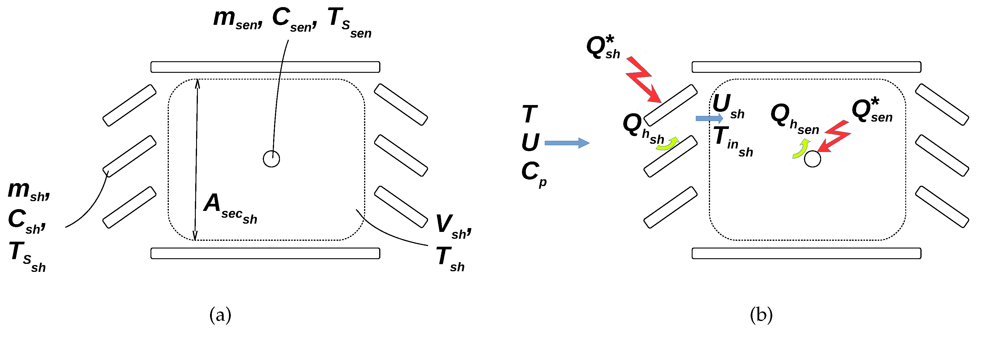
Figure 1. Cross-section view of a generic naturally ventilated shelter with (a) its main physical characteristics and (b) the main interactions with its environment.
Climate 07 00026 g001
Figure 2. Picture of the experiment site. Source: Lacombe et al. [10].
Climate 07 00026 g002
Figure 3. Disposition of the instruments within the measurement site area. Source: Lacombe et al. [10].
Climate 07 00026 g003
Figure 4. Temperature difference under different wind speed and short-wave radiation values between (a) artificially ventilated shelter VDAV1 and reference shelter SDAV, (b) LCAS and SDAV and (c) hybrid shelter VEIG and SDAV. Please note that each dot/error bars represents the median/quartiles values of a 5 percentile interval of wind speed.
Climate 07 00026 g004
Figure 5. Processing chain used for data selection.
Climate 07 00026 g005
Figure 6. Processing chain used to assess the performance of each of the models.
Climate 07 00026 g006
Figure 7. Evolution of the error within LCAS shelter against the wind speed (a) for low heating rate ( T ˙ ∼0.6 K·h 1 ) and several radiation values and (b) for low radiation ( K + K s i n Θ ∼0 W·m 2 ) and several heating rate values. Please note that each dot/error bars represents the median/quartiles values of a 5-percentile interval of wind speed.
Climate 07 00026 g007
Figure 8. Evolution of the error within LCAS shelter against the wind speed for several ϵ T ( t Δ t ) values (a) for negative heating rate ( T ˙ 1.2 K·h 1 ) and (b) for positive heating rate ( T ˙ ∼1.2 K·h 1 ). Please note that each dot/error bars represents the median/quartiles values of a 5-percentile interval of wind speed.
Climate 07 00026 g008
Figure 9. Regression coefficient p 1 versus p 0 coefficient for the entire dataset (2 Θ < 90 ). The dot corresponds to the median value of the regression coefficient. Please note that the root mean square of its median variance over the 50 regressions is low (lower than 2% of the median value).
Climate 07 00026 g009
Figure 10. Evolution of the (a) wind speed, (b) air temperature within several shelters during the night of 28 July 2008.
Climate 07 00026 g010
Figure 11. Evolution of the (a) wind speed, (b) short-wave radiation, (c) heating rate and (d) air temperature error within several shelters in 16 August 2008.
Climate 07 00026 g011
Figure 12. Values of the regression coefficients (a) p 0 and (b) p 1 for different solar angle azimuth ranges.
Climate 07 00026 g012
Figure 13. NRMSE values observed for each model and each shelter considering all day-time values. The RMSE of each shelter is indicated on the top axis.
Climate 07 00026 g013
Table 1. Shelter characteristics and physical phenomena that lead to measurement error of the air temperature.
Size and Orientation of Shield OpeningsShield Albedo & EmissivityThermal Characteristics of the Shield Structure
(Resistance, Admittance)
Direct radiationXX
Indirect radiation XX
Poor shield ventilationX
Enthalpy of phase change
(water and snow on the shelter)
X
Table 2. Main characteristics of the naturally ventilated shelters used during the WMO campaign.
AcronymManufacturerTypeNumber of SheltersLocation in Figure 3Estimated Volume V sh (dm3)Estimated Section A sec sh (dm2)Estimated Surface A sh (dm2)
LBOMBoMSmall Stevenson screen1A618036200
LCASCasellaStevenson screen1A151064380
LSOCSocrimaLarge Stevenson screen1F11000100620
SCAECAETU20AS
(Cylindric multiplate)
2C2, C5177.820
SDAVDavisPN7714
(Cuboid multiplate)
2A2, A55.62.919
SSOCSocrimaBMO1195D
(Cylindric multiplate)
2E3, E6161016
SVAIVaisalaDTR13-HMT 330 MIK
(Cylindric multiplate)
2B3, B6116.614
SWINWindspeedT351-PX-D/3
(Cylindric multiplate)
2E2, E50.500.801.8
SYOUYoung41003
(Cylindric multiplate)
2F2, F55.03.68.7
Table 3. Description of the replacement of variables originally needed in Equation (12).
Original Needed Variable (Equation (12))Substitution Variable (Measured during the WMO Campaign)Modification Brought Equation (12)
Sensor NameVariable NameSampling Conditions
U s h Wind Sonic Gill (Gill)outside wind speed UThe measurement is performed twice per second. Then a 2 min period moving-average (vectorial) is performed and only the 1 min data is recorded. * U s h = k U s h U where k U s h is a coefficient proper to each shelter
Q s h * Albedometer CMA11B
(Kipp & Zonen)
Ascending and descending short-wave radiation ( K and K )The measurement is performed once every ten seconds. Then an average of the last minute is recorded every 1 min. * Q s h * = ( 1 α ) ( K + K s i n ( Θ ) ) where α is the shelter albedo Θ is the solar zenith angle
Q s e n * Q s e n * = k K ( K + K s i n ( Θ ) ) where k K is a coefficient proper to each shelter
T ˙ PT100 temperature sensor located within the Davis PN7714 shelterOutside air temperature TThe measurement is performed once every ten seconds. Then an average of the last minute is recorded every 1 min. * T ˙ ( n ) = T ( n ) T ( n 1 ) Δ t where n 1 and n are two consecutive samples Δ t the sampling period T the outside air temperature
(*) Please note that the average is calculated and stored only under certain data quality conditions (cf. [10] for more informations.
Table 4. Monthly distribution of the available data.
Year200820082009200920092009200920092009200920092009
Month111201020304050607080910
Time step distribution (%)107.96.15.76.26.97.66.113.412.37.510.2
Table 5. Mathematical expression of the regression problems corresponding to each model.
Model NameModel FunctionExplanatory VariablesRegression Coefficients
Nakamura y = p 0 N + p 1 N x N x N = K T U p 0 N , p 1 N
Cheng y = p 0 C + p 1 C x C x C = Θ K T U p 0 C , p 1 C
Our model y = 1 p 0 O ( e p 0 O x 0 O 1 ) ( x 1 O p 1 O x 2 O ) + x 3 O · e p 0 O x 0 O x 0 O = U · Δ t ,
x 1 O = T ˙ U ,
x 2 O = K + K s i n Θ U ,
x 3 O = ϵ T ( t Δ t )
p 0 O = ζ 1 ,
p 1 O = ζ 4
Table 6. Level of magnitude of the time constant calculated using Equation (17) and observed using the 67% method during the time period identified Figure 10.
MethodLBOMSYOU2LSOC
67% method (min)2215
Equation (17) (min)1.63.313.9