Article

A Physical–Mathematical Approach to Climate Change Effects through Stochastic Resonance

by
Maria Teresa Caccamo
1 and
Salvatore Magazù
2,3,*
1
Consiglio Nazionale delle Ricerche (CNR)—Istituto per i Processi Chimico-Fisici (IPCF), Viale Ferdinando Stagno D’Alcontres n°37, S. Agata, 98166 Messina, Italy
2
Dipartimento di Scienze Matematiche e Informatiche, Scienze Fisiche e Scienze della Terra, Università di Messina, Viale Ferdinando Stagno D’Alcontres n°31, S. Agata, 98166 Messina, Italy
3
Istituto Nazionale di Alta Matematica “F. Severi”—INDAM—Gruppo Nazionale per la Fisica Matematica—GNFM, P.le Aldo Moro 5, 00185 Roma, Italy
*
Author to whom correspondence should be addressed.
Climate 2019, 7(2), 21; https://doi.org/10.3390/cli7020021
Submission received: 22 November 2018 / Revised: 15 January 2019 / Accepted: 24 January 2019 / Published: 27 January 2019

Abstract

:
The aim of this work is to study the effects induced by climate changes in the framework of the stochastic resonance approach. First, a wavelet cross-correlation analysis on Earth temperature data concerning the last 5,500,000 years is performed; this analysis confirms a correlation between the planet’s temperature and the 100,000, 41,000, and 23,000-year periods of the Milankovitch orbital cycles. Then, the stochastic resonance model is invoked. Specific attention is given to the study of the impact of the registered global temperature increase within the stochastic model. Further, a numerical simulation has been performed, based on: (1) A double-well potential, (2) an external periodic modulation, corresponding to the orbit eccentricity cycle, and (3) an increased value of the global Earth temperature. The effect of temperature increase represents one of the novelties introduced in the present study and is determined by downshifting the interaction potential used within the stochastic resonance model. The numeric simulation results show that, for simulated increasing values of the global temperature, the double-well system triggers changes, while at higher temperatures (as in the case of the absence of a global temperature increase although with a different threshold) the system goes into a chaotic regime. The wavelet analysis allows characterization of the stochastic resonance condition through the evaluation of the signal-to-noise ratio. On the basis of the obtained findings, we hypothesize that the global temperature increase can suppress, on a large time scale corresponding to glacial cycles, the external periodic modulation effects and, hence, the glacial cycles.

1. Introduction

Climate occurs as a result of processes operating on multiple scales, some of which are slow, as in the Earth’s glacial cycles, and others of which are fast, such as daily weather fluctuations [1]. Glacial cycles, on the order of tens of thousands of years, start with a gradual temperature decrease, which gives rise to an increase of sea ice, polar cap volume, and total global area occupied by ice, increasing Earth’s overall albedo and the amount of the sun’s energy reflected away from the Earth. With less energy entering the Earth’s system, temperatures decrease further, creating positive feedback. Furthermore, as more ocean water is converted to ice, the overall water volume of the oceans decreases, allowing continental submerged portions to emerge [2,3,4,5]. The equilibrium global average temperature reached by this process represents a lower stationary regime of the overall climate during that period. Glacial ages end with a temperature increase reversing the water transfer from the cryosphere back to the oceans [6,7,8,9]. Equilibrium temperature at these times represents an upper stationary regime. On the other hand, climate variations can give rise to harsh conditions that are of interest for the study of extremophile organisms [10,11,12,13] for biotechnological applications [14,15,16,17,18,19,20,21,22].
Temperature determinations performed at the Vostok scientific station (Figure 1) revealed a strong correlation with the Milankovitch cycles [23,24,25,26,27,28,29,30,31,32], and are shown in Figure 2.
In particular, the cycles correspond to: (1) an eccentricity variation of the Earth’s orbit around the Sun over a period of about 100,000 years; (2) a variation in the inclination of the Earth’s axis from a minimum of 21°55′ to a maximum of 24°20′, over a period of approximately 41,000 years; and (3) a variation of the Earth’s axis during a double-conic motion, called solar-precession, over a period of about 23,000 years [33,34,35,36,37,38,39,40,41].
Several mathematical procedures are reported in the literature to correlate in order to compare different data sets through a spectral comparison. Wavelet transform (WT) analysis is powerful tool for analysing variations of spectral power within given data series. By decomposing data sets into wavelet components, it is possible to compare the dominant signal spectral modes as well as their correlation degree. In particular, in order to highlight the correlation between the registered temperatures of Figure 1 and the mentioned Milankovitch periodicities, in this work the wavelet cross-correlation (XWT) approach has been applied [42,43,44]. Furthermore, these glacial cycles can be treated as a slow process or low-frequency climate “signal”. At this geological scale, daily temperature fluctuations can be thought of as a fast process, or a much higher-frequency signal superimposed on the glacial signal. Because the variation in solar radiation over the Milankovitch cycles alone is not able to justify temperature variation from interglacial age to glacial age, in 1980, Roberto Benzi introduced the idea that the high-frequency temperature fluctuations were a weak periodic input and a source of “noise” on the glacial signal, creating a small resonance that amplified the signal of the lower glacial frequency. He termed this hypothesis “stochastic resonance” (SR) [45,46,47,48,49,50,51,52]. Figure 3 shows a typical curve of output performance as a function of input noise magnitude.

2. Methodology

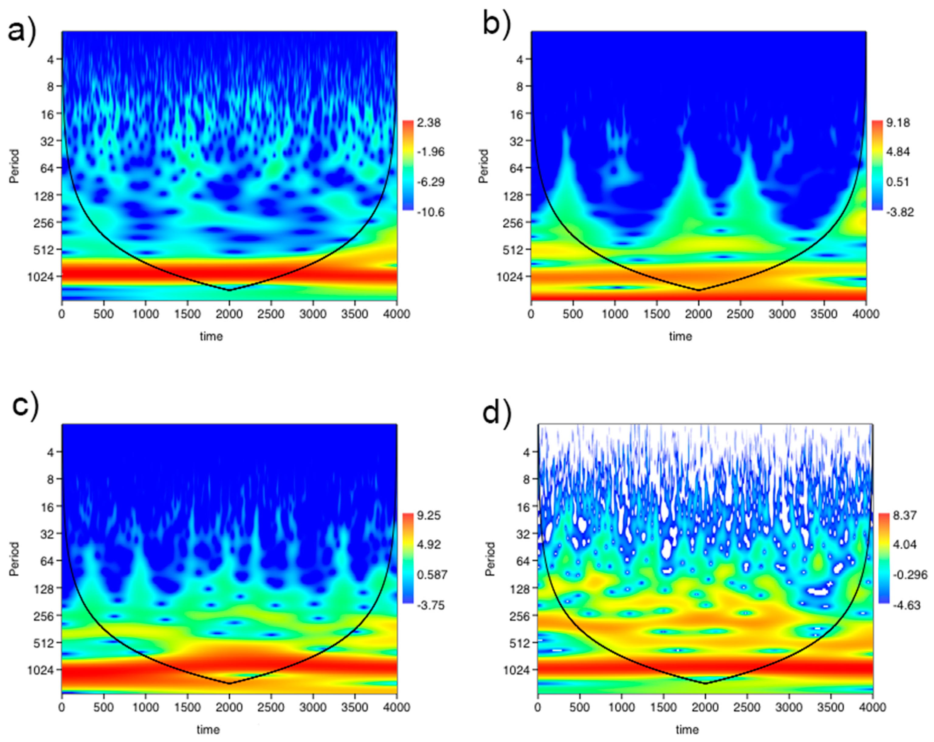
2.1. Wavelet Analysis

In order to highlight the correlation between the registered temperatures of Figure 1 and the mentioned Milankovitch periodicities, and to characterize the SR condition, in the present work we shall evaluate the wavelet cross-correlation (XWT). It is well known that wavelet tranform (WT) allows the evaluation of signal frequency and time localization. From a general viewpoint, WT assigns to function y ( x ) another function W T ( a ,   τ ) , where a , with a > 0 denotes the scale and τ a time shift [53,54,55,56,57]. Thus, WT decomposes y ( x ) into wavelets components 1 a ψ ( x τ a ) , as follows:
W T ( a ,   τ ) = 1 a + y ( x ) ψ * ( x τ a ) d t
where ψ * is the complex conjugate of the wavelet mother ψ [58,59,60,61].
Given two signals y ( x ) and g ( x ) , let us indicate W T y ( a ,   τ ) and W T g ( a ,   τ ) as their WTs, respectively. It is possible to define the cross-correlation wavelet (XWT) as:
XWT = W T y * ( a ,   τ ) W T g ( a ,   τ )
while the wavelet spectrum (WS) is:
W S ( a ) = + | W T ( a ,   τ ) | 2 d t
Since XWT allows to evaluate the degree of affinity between two signals y ( x ) and g ( x ) , in order to extract quantitative information from the signal, one can calculate the wavelet cross-correlation coefficient (CXWT):
CXWT = W T y g ( a ,   τ ) W S y ( a ) W S g ( a )
where W S y ( a ) and W S g ( a ) are the wavelet spectrum of the signal y ( x ) and g ( x ) , respectively. In order to show the effectiveness of the WT approach, the XWT between the signal and the function obtained as a sum of three in phase sinusoidal contributions with periodicities T M 1 = 2 π 100000 , T M 2 = 2 π 41000 and T M 3 = 2 π 23000 has been evaluated. In such a case, XWT, as reported in literature, allows us to highlight existing correlations, both in terms of spectral power and of relative phase, in the time–frequency space. Figure 4 reports the results of such a XWT evaluation that shows a noticeable level of correlation which increases for the most recent times [62,63,64,65].
The arrows in the figure indicate the phase relationship between the two series. The colour bar indicates the strength of the wavelet power. The redder it appears in the scalogram, the more power the spectra contains at that particular scale. In the following the WT approach will be employed to characterize the SR condition.

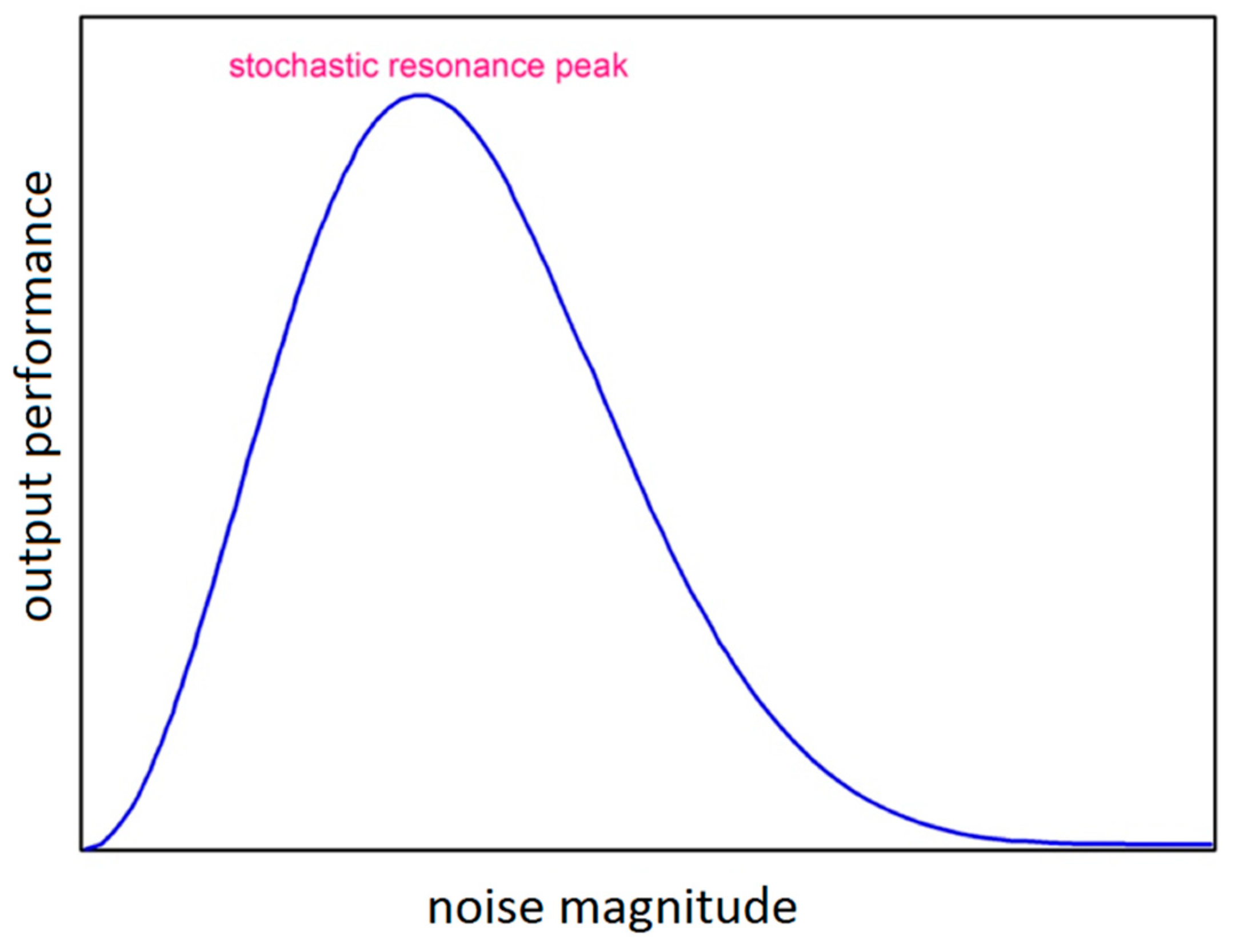
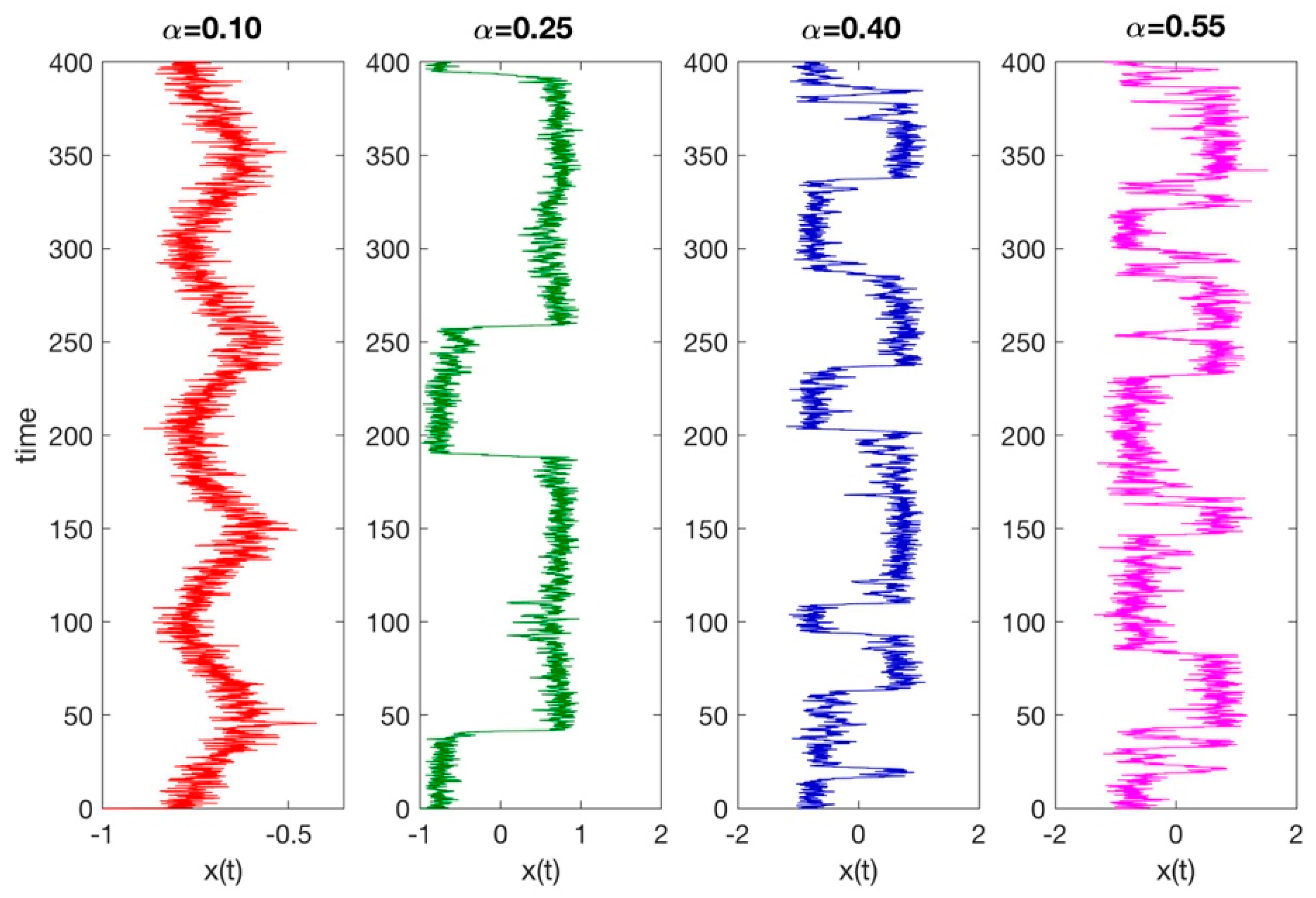
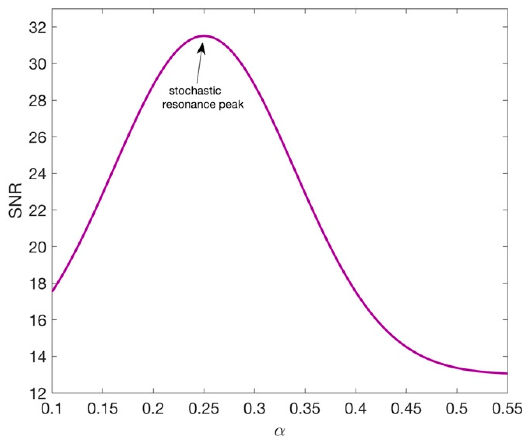
2.2. Stochastic Resonance

Let us consider now a system that can be modelled as a particle of mass m whose position is x(t) (particle space coordinate), moving in a potential V(x) and on which a friction force is exerted proportional to its velocity, i.e., f f r i c t i o n = ζ d x ( t ) d t (Stokes force), and a random force, f r a n d o m = ξ ( t ) , connected with the “heat bath” in which the particle moves. The particle motion equation is:
m d 2 x ( t ) d t 2 = d V ( x ) d x ζ d x ( t ) d t + ξ ( t )
The term ξ ( t ) makes this differential equation a stochastic one. We assume the particle moves in the “high friction limit” where the acceleration is negligible, and absorbing the constant γ into the potential function V(x) and the random force ξ ( t ) , one has:
d x ( t ) d t = d V ( x ) d x + ξ ( t )
SR is termed a phenomenon that occurs in nonlinear systems whereby a weak signal is amplified and optimized by the assistance of noise.
The effect requires three basic ingredients:
(1)
a non-linear system characterized by an energetic activation barrier or, more generally, by a form of threshold;
(2)
a weak input;
(3)
a source of noise that is inherent in the system, or that adds to the input.
Given these features, the response of the system undergoes to a resonance-like behaviour as a function of the noise level.
An example of signal performance parameter is furnished by the output signal-to-noise ratio (SNR). In particular, the SNR against input noise amplitude/intensity, as reported in Figure 3, shows a single maximum at a nonzero value similar to frequency-dependent systems that have a maximum SNR, or output response, for some resonant frequency. However, in the case of SR, the resonance is ‘‘noise-induced’’ rather than at a particular frequency [66,67].
It should be stressed that for linear signal-processing systems, the output SNR is maximized in the absence of noise; therefore, noise is not beneficial in a linear system, since only the interactions between nonlinearities and randomness can lead to SR [45,46,47,48].
In its classical setting, SR applies to bistable nonlinear dynamical systems subject to noise and periodic forcing [68,69]. Taking into account the Langevin equation, a generic equation form for these types of systems is:
d x d t = d V d x + ξ ( t ) + ε cos ( ω 0 t + φ )
where the periodic forcing term, having a pulsation ω 0 , is given by ε cos ( ω 0 t + φ ) ; for simplicity, in the following we assume that the phase shift φ = 0 . To figure out what SR is, it can be useful to consider the canonical example first put forth by McNamara et al. [70] by introducing the symmetric bistable potential well given by:
V ( x ) = a 2 x 2 + b 4 x 4
This potential shows two stable equilibrium points at x ± = ± c = ± a b , and an unstable equilibrium at x = 0 . Let V 0 be the height of the potential when ε = 0 ; V 1 = ε c be the amplitude of the modulation in barrier height when the periodic force is turned on; and ξ ( t ) be a zero mean Gaussian white noise with intensity D and an autocorrelation function. A delta function, δ ( t ) , is given by:
< ξ ( t ) ξ ( 0 ) 2 D δ ( t )
When no periodic force is present, i.e., when ε = 0 , the behaviour of the system is characterized by a x ( t ) function which, depending on the involved parameter values, can fluctuate around the minima with a variance proportional to D , making random noise-induced hops from one well to the other. As we shall see, under specific circumstances, the introduction of a periodic force makes the transition probability of escaping from each well varying in time.

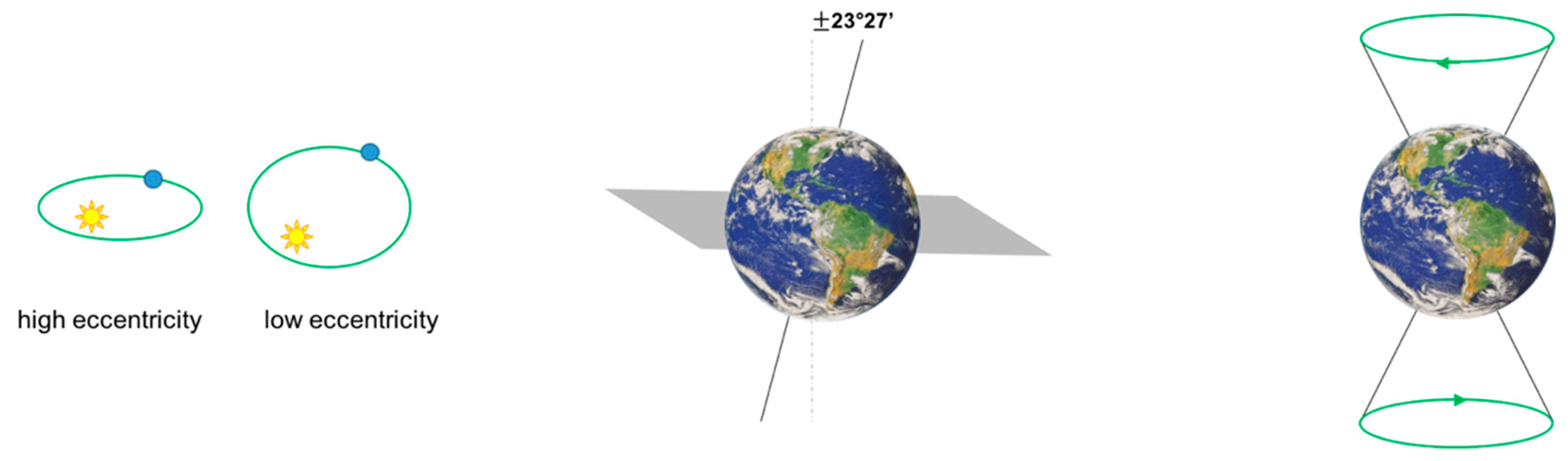
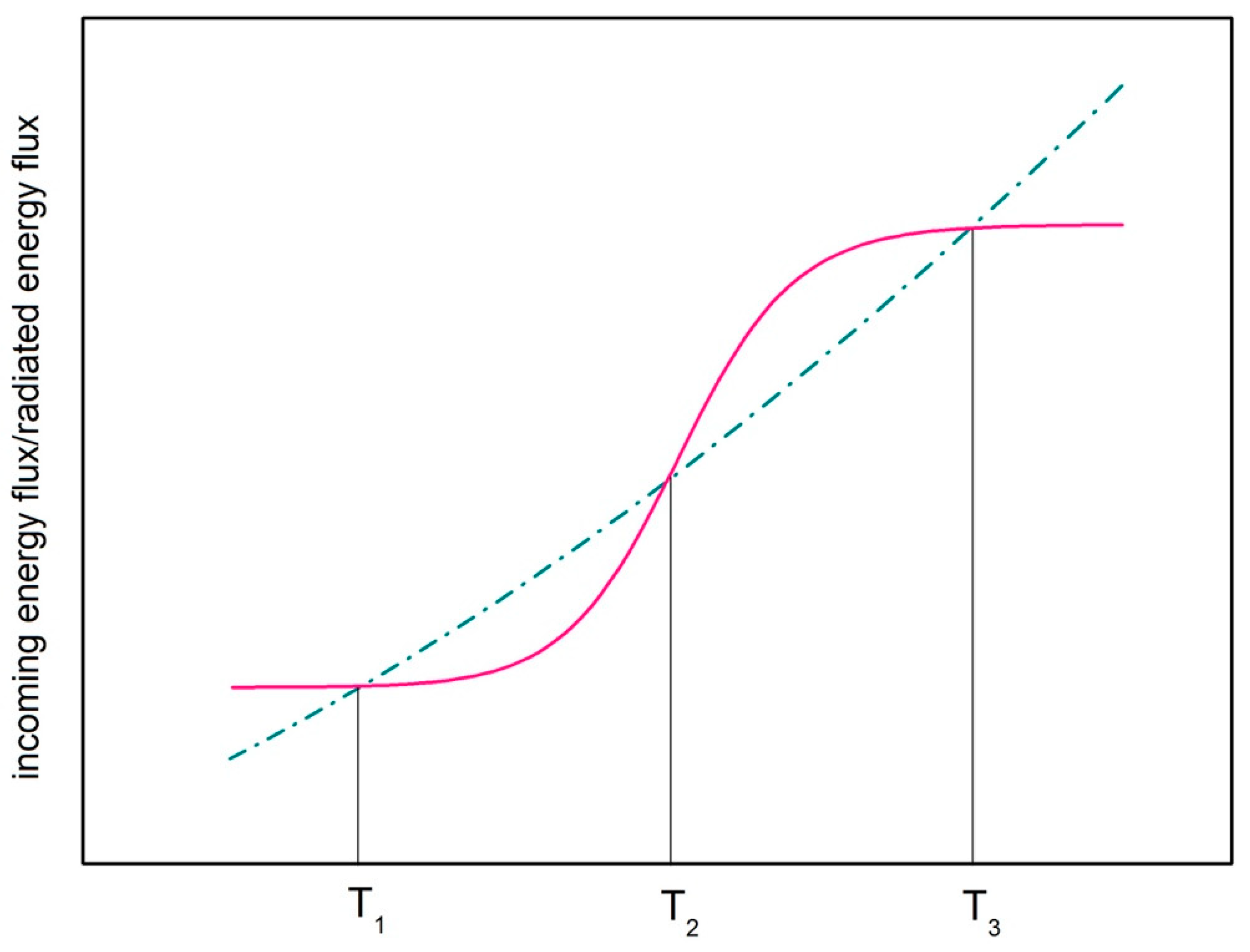
2.3. Slow and Fast Processes of Earth’s Energy Balance
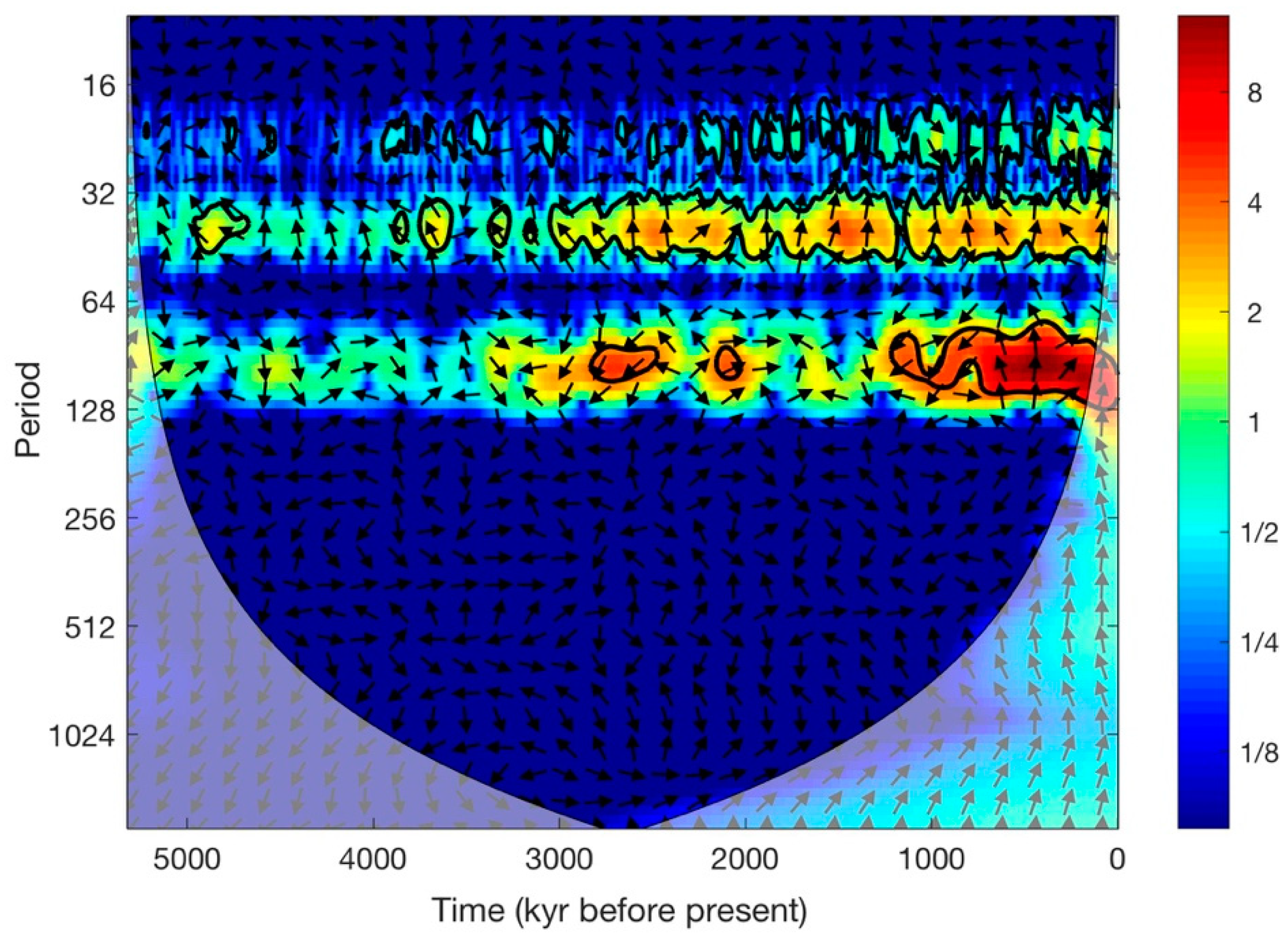
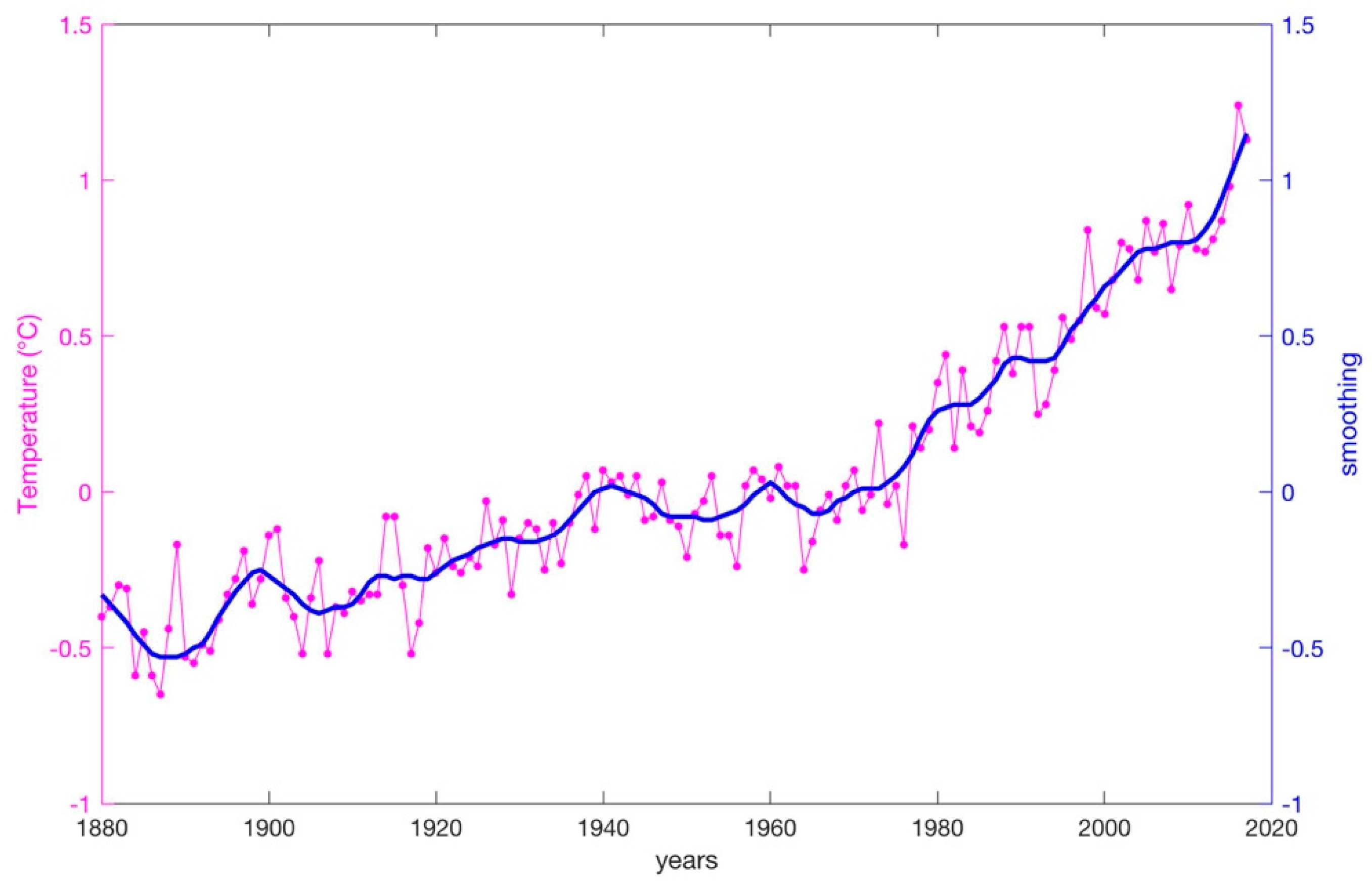
Following the Budyko–Sellers model [71,72,73,74,75], the Earth’s temperature time variation can be evaluated by taking into account the energy balance between the incoming ( R i n ), and outcoming ( R o u t ), radiation:
c d T d t = R i n R o u t
where c is the Earth thermal capacity.
By R i n and R o u t , one can express Equation (18) in terms of a temperature-dependent potential V:
c d T d t = V T
This implies that the stationary solutions of this equation are the minima or maxima of the potential V, occurring in correspondence to stable and to unstable configurations, respectively. It should be noted that Equation (19) does not take into account fast processes connected to meteorological fluctuations due to atmospheric dynamics and circulation (of the order of months or years). We can consider these fast variables as noise acting on the slow variables (varying on a time scale of the order of thousands of years); under such circumstances, the slow variable is the temperature, whose overall variation is considered over a time window of million years. Finally, including the fast processes, the equation becomes [45,46,47,48]:
d T = 1 c V T d t + α d η ( t )
where α represents the intensity of the stochastic noise and η ( t ) is a stochastic function describing the short time scale processes connected with atmospheric dynamics and circulation.
To simulate the behaviour of such an equation, at first we neglect the stochastic noise and build V T , parameterizing R i n and R o u t ; after this we estimate the intensity of meteorological noise.
To take into account the effect of the periodic variation of the eccentricity that varies the solar constant, we use for R i n the following formula:
R i n = Q ( 1 + A cos ω t )
where Q is the solar constant, A is the amplitude of the modulation that as calculated by Milanković, is 5 × 10⁻⁴ and corresponds to an overall variation of Q of 0.1% over a period of about 11 years, and ω = 2 π / T with T = 100,000 years. The outgoing radiation, R o u t , can be parameterized as the sum of two contributions, one corresponding to the reflected solar radiation and one corresponding to the component radiated from the Earth according to its temperature, i.e., E ( T ) = 4 π R 2 σ T 4 :
R o u t = μ ( T ) R i n + E ( T )
with μ ( T ) coefficient representing the fraction of incident radiation reflected in all directions known as albedo [4]. Replacing Equations (21) and (22) into Equation (18), it follows that:
c d T d t = Q ( 1 + A cos ω t ) ( 1 μ ( T ) ) E ( T )
Now, we examine some qualitative properties of Equation (15), basing our remarks on the well-established mathematics of Budyko–Sellers models.
Assuming that A = 0, Equation (15) becomes c d T d t = Q ( 1 μ ( T ) ) E ( T ) . Let us compare these two contributions in Figure 5. Here the dotted-dashed green line represents the black body law, while the continuous pink line represents absorbed radiation, that is, the solar constant modulated by the effect of the albedo. The intersections between the two curves define the equilibrium points of the system in which, by definition d T / d t = 0 , while their stability is determined by the potential second derivatives.
Let us assume that T3 is the actual planet average temperature, which is about 288.6 K; furthermore, be T1 = 278.6 K and T2 = 283.3 K the glacial state and the average temperature respectively, the stationary solutions will be determined by the condition Q ( 1 μ ( T ) ) = E ( T ) . We introduce the function γ ( T ) = ( Q ( 1 μ ( T ) ) E ( T ) 1 ) 1 , defined by the conditions γ ( T ) = 0 when T = T i with i = 1, 2, 3.
Then, in the temperature range under investigation, γ ( T ) can be modelled as γ ( T ) = β ( 1 T T 1 ) ( 1 T T 2 ) ( 1 T T 3 ) , where β is a constant parameter. Then, by inserting the obtained quantities into Equation (15), which takes into account the external periodic perturbation, one obtains:
d T d t = E ( T ) c = [ β ( 1 T T 1 ) ( 1 T T 2 ) ( 1 T T 3 ) ( 1 + A cos ω t ) + A cos ω t ]
where the potential (see Equation (20) for a comparison) is a time-dependent function.
Finally, by adding the noise contribution [45,46,47,48] to Equation (16):
d T d t = E ( T ) c = [ β ( 1 T T 1 ) ( 1 T T 2 ) ( 1 T T 3 ) ( 1 + A cos ω t ) + A cos ω t ] + α d η ( t )
it is possible to study, through Equation (17), the total system response.
Before proceeding, it is possible to evaluate the temperature variation in the absence of noise i.e., for α = 0 ; in particular, for numerical values E = 8.77 × 10 3   W and c = 4000 J/K, a variation of 0.3 K (compatible with the results of other investigations). Evidently, this result is not compatible with the observed variation of 10K. Therefore, one has to conclude that the only periodical perturbation is not sufficient for the system to pass from one stable state to the another one (i.e., from T3 to T1 and vice versa); furthermore, the astronomical modulations move the curves reported in Figure 5 very little, and therefore the fixed points are kept [45,46,47,48].
What emerges is that from the simulation of Equation (17) and varying the noise, for certain values of α the jump from T3 to T1 and vice versa occurs in sync with the frequency (resonance condition) of the periodic signal; therefore, this result is able to reproduce the characteristic periodicity of the ice ages and the corresponding temperature difference. Furthermore, the noise value is compatible with the current temperature fluctuations around the climatic average which is about 0.1 K2/year [45,46,47,48]. The transition between the two stable configuration rests is a probabilistic event; this implies that if the transition between the two states does not occur, the system has to wait for another cycle to obtain the same resonant condition.

3. Results

In the following we will present at first the outputs of a numerical simulation investigation for a system characterized by a double well potential to which is added a small periodic contribution; the study is performed by taking into account different weights for the noise. Then, to simulate the effects of the temperature rise in the framework of the stochastic resonance approach, we will show the results of a simulation for a system characterized by a down-shifted double well potential.
Let us first introduce a simple double-well potential which now includes the small periodic contribution:
V ( x , t ) = x 4 x 2 + a x cos ( ω t )
Then Equation (6) can be written as:
d x = V x d t + α d η ( t )
where α and η ( t ) , describe the stochastic noise. As above stated, depending on the α values, this latter contribution can amplify the Milankovic cycle signal. The simulation of Equation (19) has been performed by varying the intensity of the noise while keeping the periodic signal constant. As a result, we observe that there is a certain noise value, i.e., a value for α , for which the jump of the system from one hole to the other is synchronized with the frequency of the external signal as reported in Figure 6 (i.e., the so-called resonance condition). More precisely, Figure 6 reports the solution of Equation (19) for a = 0.3 and α = 0.10 ,   0.25 ,   0.40 , 0.55. For α = 0.10 , the system is confined in the left well while for α = 0.25 it jumps to the right well, starting a periodic oscillation between the two wells; for α = 0.40 and α = 0.55, the resonance efficiency decreases.
In order to characterize the stochastic resonance condition, we have evaluated the WT scalograms (see Figure 7) relative to the solutions of Equation (19) for a = 0.3 and α = 0.10   ( a ) ,   0.25 ( b ) ,   0.40 (c) and 0.55 (d).
It should be noticed, as shown in figure, that the transition from one stable state to the other one is a probabilistic event and hence, also under the resonance condition, the system jump between the two states is not certain; furthermore, when that the transition between the two states does not occur, the system has to wait for another cycle to get the same resonant condition.
Furthermore, by means of WT it is possible to extract quantitatively the value of the signal-to-noise ratio, shown in Figure 8. What it emerges is that the SNR shows a maximum for a = 0.3 and α = 0.25   ( b ) .
In the following we shall investigate in this scenery the outcomes of the stochastic model for increasing values of the global planet temperature. More specifically, it is well known that temperature determinations in the Earth’s atmosphere, in oceans, and on our planet’s surface indicate an increased warming process starting from the nineteenth century [76,77]. Figure 9 shows the global temperature trend which shows how, starting from 1970, the slope of the regression line is undergoing a substantial increase, which brings the heating values between 1970 and 2017 to about 0.17 °C/decade. It is therefore meaningful to investigate which effects can be generated by such a global temperature rise in the framework of the above discussed SR model.
In order to simulate the effects of the temperature rise in the framework of the stochastic resonance approach, we have performed a new numerical simulation for a system characterized by a down-shifted double-well potential to which a small periodic contribution is added, i.e., V ( x , t ) = x 4 x 2 V 0 + a x cos ( ω t ) ; again the study is performed by taking into account different weights for the noise.
Figure 10 shows the solution of Equation (19) for V 0 = 2 when the amplitude of the external periodic perturbation is a = 0.3 and the noise level is α = 0.10 ,   0.40 , and 0.80. On the top of the figure the potential double-well is shown, while on the respective bottom, the particle position (horizontal axis) as a function of time (vertical axis) is shown. As can be seen, for α = 0.10 (case a), the system is confined in the left well; however, for α = 0.40 (case b), the particle jumps from the one well to the other one in synchrony with the external perturbation a cos ( ω t ) ; a further noise increase, i.e., at α = 0.8 , (case c), gives rise to a diminishing of the resonance efficiency.
Figure 11a shows a comparison between the two analysed configurations, i.e., for V 0 = 0 on the left and V 0 = 2 on the right for a = 0.3. In particular while for V 0 = 0 the jump threshold occurs at a noise level of α = 0.21 , for V 0 = 2 the jump threshold occurs at α = 0.19.
The present study clearly shows that the registered planet temperature increase could give rise to effects similar to those connected with a high noise value. Therefore, in the framework of the SR approach, the global temperature increase corresponds to a downshift of the system potential energy, which in turn can justify the registered increase in the frequency of the planet extreme weather events, such as extreme heat, intense precipitation, and drought, which have become more frequent and severe in recent decades.
In particular, the evidence of global climate change based on the analysis of the long-term variability that affects the different components of the climate system (atmosphere, oceans, cryosphere, etc.) indicates unequivocally that since the nineteenth century the planet has undergone a warming process. In fact, in recent decades, soil and ocean temperatures have increased not homogeneously, but with greater warming near polar latitudes, especially in the Arctic region. The ice and snow coverage has decreased in different areas of the planet. The atmospheric water vapor content has increased everywhere due to the higher temperature of the atmosphere while sea level has also increased. Furthermore, changes in other climatic indicators have also been observed, such as seasonal elongation in many places on the planet, often accompanied by an increase in the tendency of extreme events such as heat waves or heavy rainfall and a general decrease in extreme cold events. Most of the warming observed globally over the last 50 years, as well as the increase of the registered extreme events, could be explained if one considers the effect produced by human activities and in particular both the emissions from fossil fuels and the deforestation process in the framework of the stochastic resonance effect in the presence of augmented thermal energy on the planet.

4. Conclusions

Climate change phenomena connected to the registered global increase of temperature within the framework of the SR approach are analysed by means of XWT and numeric simulations and then discussed.
In particular, a XWT analysis was performed to highlight the correlation between the planet’s temperature and the 105-, 41 × 103-, and 23 × 103-year periodicities of the Milankovitch orbital cycles. Then, the well-known SR model applied to the interpretation of climate cycles is discussed. In this framework, the WT analysis allows us to characterize the stochastic resonance condition through the evaluation of the signal-to-noise ratio. Furthermore, a specific study of the feedbacks induced by a global temperature increase on SR previsions has been performed by taking into account a downshift of the system’s potential well within the SR model. In particular, a mathematical simulation was performed taking into account a double-well potential, an external periodic modulation corresponding the Milankovitch’s cycle, and increasing values of thermal energy values for the planet. The study puts into evidence different triggering between the two regimes and suggests that the higher Earth temperature values, mainly attributed to human activities, could induce an increase both in the number and intensity of extreme weather events. Future directions of study will concern the global warming of the Earth’s climate system due to human activities, i.e., global warming, when triggered by internal forcing mechanisms, i.e., periodic internal parameter variations.

Author Contributions

Formal analysis, M.T.C. and S.M.; Writing—original draft, M.T.C. and S.M.; Writing—review & editing, M.T.C. and S.M.

Funding

This research received no external funding.

Conflicts of Interest

The authors declare no conflict of interest.

References

  1. Benzi, R. Stochastic resonance: From climate to biology. Nonlinear Proc. Geophs. 2010, 17, 431–441. [Google Scholar] [CrossRef]
  2. Jacka, T.H.; Budd, W.F. Detection of temperature and sea-ice-extent changes in the Antarctic and Southern Ocean, 1949–1996. Ann. Glaciol. 1998, 27, 553–559. [Google Scholar] [CrossRef]
  3. Caccamo, M.T.; Castorina, G.; Colombo, F.; Insinga, V.; Maiorana, E.; Magazù, S. Weather forecast performances for complex orographic areas: Impact of different grid resolutions and of geographic data on heavy rainfall event simulations in Sicily. Atmos. Res. 2017, 198, 22–33. [Google Scholar] [CrossRef]
  4. Grinsted, A.; Moore, J.C.; Jevrejeva, S. Reconstructing sea level from paleo and projected temperatures 200 to 2100 AD. Clim. Dyn. 2010, 34, 461–472. [Google Scholar] [CrossRef]
  5. Calabrò, E.; Magazù, S. Correlation between increases of the annual global solar radiation and the ground albedo solar radiation due to desertification-A possible factor contributing to climatic change. Climate 2016, 4, 64. [Google Scholar] [CrossRef]
  6. Monnin, E.; Indermuhle, A.; Dallenbach, A.; Fluckiger, J.; Stauffer, B.; Stocker, T.F.; Raynaud, D.; Barnola, J.-M. Atmospheric CO2 Concentrations over the Last Glacial Termination. Science 2001, 291, 112–114. [Google Scholar] [CrossRef] [PubMed]
  7. Nakamura, K.; Doi, K.; Shibuya, K. Estimation of seasonal changes in the flow of Shirase Glacier using JERS-1/SAR image correlation. Polar Sci. 2007, 1, 73–84. [Google Scholar] [CrossRef]
  8. Davey, M.C. Effects of continuous and repeated dehydration on carbon fixation by bryophytes from the maritime Antarctic. Oecologia 1997, 110, 25–31. [Google Scholar] [CrossRef]
  9. Caccamo, M.T.; Calabrò, E.; Cannuli, A.; Magazù, S. Wavelet Study of Meteorological Data Collected by Arduino-Weather Station: Impact on Solar Energy Collection Technology”. MATEC Web Conf. 2016, 55, 02004. [Google Scholar] [CrossRef]
  10. Raper, S.C.; Wigley, T.M.; Jones, P.D.; Salinger, M.J. Variations in surface air temperatures: Part 3. The Antarctic, 1957–1982. Mon. Weather Rev. 1984, 112, 1341–1353. [Google Scholar] [CrossRef]
  11. Babalola, O.O.; Kirby, B.M.; Le Roes-Hill, M.; Cook, A.E.; Cary, S.C.; Burton, S.G.; Cowan, D.A. Phylogenetic analysis of actinobacterial populations associated with Antarctic Dry Valley mineral soils. Environ. Microb. 2009, 11, 566–576. [Google Scholar] [CrossRef] [PubMed] [Green Version]
  12. Jones, P.D. Recent variations in mean temperature and the diurnal temperature range in the Antarctic. Geophys. Res. Lett. 1995, 22, 1345–1348. [Google Scholar] [CrossRef]
  13. Jones, P.D.; Mann, M.E. Climate Over Past Millennia. Rev. Geophys. 2004, 42, RG2002. [Google Scholar] [CrossRef]
  14. Bailey, D.M.; Johnston, I.A.; Peck, L.S. Invertebrate muscle performance at high latitude: Swimming activity in the Antarctic scallop Adamussium colbecki. Polar Biol. 2005, 28, 464–469. [Google Scholar] [CrossRef]
  15. Stark, J.S.; Snape, I.; Riddle, M.J. Abandoned Antarctic waste disposal sites: Monitoring remediation outcomes and limitations at Casey Station. Ecol. Manag. Restor. 2006, 7, 21–31. [Google Scholar] [CrossRef]
  16. Moberg, A.; Sonechkin, D.M.; Holmgren, K.; Datsenko, N.M.; Karlén, W. Highly variable Northern Hemisphere temperatures reconstructed from low- and high-resolution proxy data. Nature 2005, 433, 613–617. [Google Scholar] [CrossRef] [PubMed]
  17. Azam, F.; Beers, J.R.; Campbell, L.; Carlucci, A.F.; Holm-Hansen, O.; Reis, F.M.H.; Karl, D.M. Occurrence and metabolic activity of organisms under the Ross Ice Shelf, Antarctica, at station J9. Science 1979, 203, 451–453. [Google Scholar] [CrossRef] [PubMed]
  18. Colombo, F.; Caccamo, M.T.; Magazù, S. Trehalose Based Extremophiles in Harsh Environments. In Trehalose: Sources, Chemistry and Applications; Nova Publishers: New York, NY, USA, 2019. [Google Scholar]
  19. Lokotosh, T.V.; Magazù, S.; Maisano, G.; Malomuzh, N.P. Nature of Self-Diffusion and Viscosity in Supercooled Liquid Water. Phys. Rev. E 2000, 62, 3572–3580. [Google Scholar] [CrossRef]
  20. Magazù, S.; Migliardo, F.; Telling, M.T.F. Structural and dynamical properties of water in sugar mixtures. Food Chem. 2008, 106, 1460–1466. [Google Scholar] [CrossRef]
  21. Migliardo, F.; Caccamo, M.T.; Magazù, S. Elastic Incoherent Neutron Scatterings Wavevector and Thermal Analysis on Glass-forming Homologous Disaccharides. J. Non-Cryst. Solids 2013, 378, 144–151. [Google Scholar] [CrossRef]
  22. Magazù, S.; Migliardo, F.; Caccamo, M.T. Innovative Wavelet Protocols in Analyzing Elastic Incoherent Neutron Scattering. J. Phys. Chem. B 2012, 116, 9417–9423. [Google Scholar] [CrossRef] [PubMed]
  23. Barnola, J.-M.; Raynaud, D.; Korotkevich, Y.S.; Lorius, C. Vostok ice core provides 160,000-year record of atmospheric CO2. Nature 1987, 329, 408–441. [Google Scholar] [CrossRef]
  24. Jouzel, J.; Lorius, C.; Petit, J.R.; Genthon, C.; Barkov, N.I.; Kotlyakov, V.M.; Petrov, V.M. Vostok ice core: A continuous isotopic temperature record over the last climatic cycle (160,000 years). Nature 1987, 329, 403–408. [Google Scholar] [CrossRef]
  25. Pepin, L.; Raynaud, D.; Barnola, J.-M.; Loutre, M.F. Hemispheric roles of climate forcings during glacial-interglacial transitions as deduced from the Vostok record and LLN-2D model experiments. J. Geophys. Res. 2001, 106, 31:885–31:892. [Google Scholar] [CrossRef]
  26. Petit, J.R.; Basile, I.; Leruyuet, A.; Raynaud, D.; Lorius, C.; Jouzel, J.; Stievenard, M.; Lipenkov, V.Y.; Barkov, N.I.; Kudryashov, B.B.; et al. Four climate cycles in Vostok ice core. Nature 1997, 387, 359–360. [Google Scholar] [CrossRef] [Green Version]
  27. Basile, I.; Grousset, F.E.; Revel, M.; Petit, J.R.; Biscaye, P.E.; Barkovd, N.I. Patagonian origin dust deposited in East Antarctica (Vostok and Dome C) during glacial stages 2, 4 and 6. Earth Planet. Sci. Lett. 1997, 146, 573–589. [Google Scholar] [CrossRef]
  28. Becker, J.; Lourens, L.J.; Hilgen, F.J.; van der Laan, E.; Kouwenhoven, T.J.; Reichart, G.J. Late Pliocene climate variability on Milankovitch to millennial time scales: A high-resolution study of MIS100 from the Mediterranean. Palaeogeogr. Palaeocl. 2005, 228, 338–360. [Google Scholar] [CrossRef] [Green Version]
  29. Lachniet, M.; Asmerom, Y.; Polyak, V.; Denniston, R. Arctic cryosphere and Milankovitch forcing of Great Basin paleoclimate. Sci. Rep. 2017, 7, 12955. [Google Scholar] [CrossRef] [Green Version]
  30. Petit, J.R.; Jouzel, J.; Raynaud, D.; Barkov, N.I.; Barnola, J.-M.; Basile, I.; Benders, M.; Chappellaz, J.; Davis, M.; Delayque, G.; et al. Climate and atmospheric history of the past 420,000 years from the Vostok ice core. Antarctica. Nat. 1999, 399, 429–436. [Google Scholar]
  31. Lisiecki, L.E.; Raymo, M.E. A Pliocene-Pleistocene stack of 57 globally distributed benthic d18O records. Paleoceanography 2005, 20, PA1003. [Google Scholar]
  32. Milankovitch, M. Canon of Insolation and the Ice Age Problem; Zavod za Udz benike i Nastavna Sredstva: Belgrade, Serbia, 1941. [Google Scholar]
  33. Petit, J.R.; Mounier, L.; Jouzel, J.; Korotkevitch, Y.S.; Kotlyakov, V.I.; Lorius, C. Paleoclimatological implications of the Vostok core dust record. Nature 1990, 343, 56–58. [Google Scholar] [CrossRef]
  34. Waelbroeck, C.; Jouzel, J.; Labeyrie, L.; Lorius, C.; Labracherie, M.; Stiévenard, N.; Barkov, N.I. A comparison of the Vostok ice deuterium record and series from Southern Ocean core MD 88-770 over the last two glacial-interglacial cycles. Clim. Dyn. 1995, 12, 113–123. [Google Scholar] [CrossRef]
  35. Suwa, M.; Bender, M.L. Chronology of the Vostok ice core constrained by O2/N2 ratios of occluded air, and its implication for the Vostok climate records. Quaternary Sci. Rev. 2008, 27, 1093–1106. [Google Scholar] [CrossRef]
  36. Landais, A.; Barkan, E.; Luz, B. Record of delta δ18O and 17O-excess in ice from Vostok Antarctica during the last 150,000 years. Geophys. Res. Lett. 2008, 35, L02709. [Google Scholar]
  37. Bopp, L.; Kohfeld, K.E.; Le Quere, C.; Aumont, O. Dust impact on marine biota and atmospheric CO2 during glacial periods. Paleoceanography 2003, 18, 1046. [Google Scholar] [CrossRef]
  38. Farquhar, G.D.; Lloyd, J.; Taylor, J.A.; Flanagan, L.B.; Syvertsen, J.P.; Hubick, K.T.; Wong, S.C.; Ehleringer, J.R. Vegetation effects on the isotope composition of oxygen in atmospheric CO2. Nature 1993, 363, 439–442. [Google Scholar] [CrossRef]
  39. Bargagli, R.; Agnorelli, C.; Borghini, F.; Monaci, F. Enhanced deposition and bioaccumulation of mercury in Antarctic terrestrial ecosystems facing a coastal polynya. Environ. Sci. Technol. 2005, 39, 8150–8155. [Google Scholar] [CrossRef]
  40. Richardson, A.J.; Schoeman, D.S. Climate impact on ecosystems in the northeast Atlantic. Science 2004, 305, 1609–1612. [Google Scholar] [CrossRef]
  41. Imbrie, J.; Boyle, E.A.; Clemens, S.C.; Duffy, A.; Howard, W.R.; Kukla, G.; Toggweiler, J.R. On the Structure and Origin of Major Glaciation Cycles 1. Linear Responses to Milankovitch Forcing. PALOC 1992, 7, 701–738. [Google Scholar] [CrossRef]
  42. Li, H.; Nozaki, T. Wavelet cross-correlation analysis and its application to a plane turbulent jet. Int. J. Ser. B 1997, 40, 58–66. [Google Scholar] [CrossRef]
  43. Caccamo, M.T.; Magazù, S. Ethylene Glycol—Polyethylene Glycol (EG-PEG) Mixtures: Infrared Spectra Wavelet Cross-Correlation Analysis. Appl. Spectrosc. 2017, 71, 401–409. [Google Scholar] [CrossRef]
  44. Grinsted, A.; Moore, J.C.; Jevrejeva, S. Application of the cross wavelet transform and wavelet coherence to geophysical time series. Nonlinear Proc. Geoph. 2004, 11, 561–566. [Google Scholar] [CrossRef] [Green Version]
  45. Benzi, R.; Sutera, A.; Vulpiani, A. The mechanism of stochastic resonance. J. Phys. A 1981, 14, L453–L457. [Google Scholar] [CrossRef] [Green Version]
  46. Bulsara, A.R.; Dari, A.; Ditto, W.L.; Murali, K.; Sinha, S. Logical stochastic resonance. Chem. Phys. 2010, 375, 424–434. [Google Scholar] [CrossRef]
  47. Benzi, R.; Parisi, G.; Sutera, A.; Vulpiani, A. Stochastic resonance in climatic change. Tellus 1982, 34, 10–16. [Google Scholar] [CrossRef]
  48. Hänggi, P.; Inchiosa, M.E.; Fogliatti, D.; Bulsara, A.R. Nonlinear stochastic resonance: The saga of anomalous output-input gain. Phys. Rev. E 2000, 62, 6155–6163. [Google Scholar] [CrossRef]
  49. Gammaitoni, L.; Hänggi, P.; Jung, P.; Marchesoni, F. Stochastic resonance: A remarkable idea that changed our perception of noise. Eur. Phys. J. B 2009, 69, 1–3. [Google Scholar] [CrossRef]
  50. Berdichevsky, V.; Gitterman, M. Stochastic resonance in linear systems subject to multiplicative and additive noise. Phys. Rev. E 1999, 60, 1494–1499. [Google Scholar] [CrossRef]
  51. Li, J.H.; Han, Y.X. Phenomenon of stochastic resonance caused by multiplicative asymmetric dichotomous noise. Phys. Rev. E 2006, 74, 051115. [Google Scholar] [CrossRef]
  52. Gammaitoni, L.; Bulsara, A.R. Nonlinear sensors activated by noise. Phys. A 2003, 325, 152–164. [Google Scholar] [CrossRef]
  53. Caccamo, M.T.; Magazù, S. Variable mass pendulum behaviour processed by wavelet analysis. Eur. J. Phys. 2017, 38, 15804. [Google Scholar] [CrossRef]
  54. Prokoph, A.; Patterson, R.T. Application of wavelet and discontinuity analysis to trace temperature changes: Eastern Ontario as a case study. Atmos. Ocean 2004, 42, 201–212. [Google Scholar] [CrossRef]
  55. Mallat, S.G. A theory for multiresolution signal decomposition: The wavelet representation. IEEE Trans. Pattern Anal. Mach. Intell. 1989, 11, 674–693. [Google Scholar] [CrossRef]
  56. Caccamo, M.T.; Cannuli, A.; Magazù, S. Wavelet analysis of near-resonant series RLC circuit with time-dependent forcing frequency. Eur. J. Phys. 2017, 38, 015804. [Google Scholar] [CrossRef]
  57. Daubechies, I. The wavelet transform, time-frequency localization and signal analysis. IEEE Trans. Inf. Theory 1990, 36, 961–1005. [Google Scholar] [CrossRef]
  58. Morlet, J.; Arens, G.; Fourgeau, E.; Glard, D. Wave propagation and sampling theory; Part I, Complex signal and scattering in multilayered media. Geophysics 1982, 47, 203–221. [Google Scholar] [CrossRef]
  59. Caccamo, M.T.; Magazù, S. Variable length pendulum analyzed by a comparative Fourier and wavelet approach. Revista Mexicana de Fisica E 2018, 64, 81–86. [Google Scholar]
  60. Kronland-Martinet, R.; Morlet, J.; Grossmann, A. Analysis of sound patterns through wavelet transform. Int. J. Pattern Recogn. 1987, 1, 97–126. [Google Scholar] [CrossRef]
  61. Caccamo, M.T.; Magazù, S. Thermal restraint on PEG-EG mixtures by FTIR investigations and wavelet cross-correlation analysis. Polym. Test. 2017, 62, 311–318. [Google Scholar] [CrossRef]
  62. Crucifix, M. Oscillators and relaxation phenomena in Pleistocene climate theory. Philosoph. Trans. R. Soc. A 2012, 370, 1140–1165. [Google Scholar] [CrossRef] [Green Version]
  63. Razdan, A. Wavelet Correlation Coefficient of ‘strongly correlated’ financial time series. Phys. A 2004, 333, 335–342. [Google Scholar] [CrossRef]
  64. Caccamo, M.T.; Magazù, S. Tagging the oligomer-to-polymer crossover on EG and PEGs by infrared and Raman spectroscopies and by wavelet cross-correlation spectral analysis. Vib. Spectrosc. 2016, 85, 222–227. [Google Scholar] [CrossRef]
  65. Veleda, D.; Montagne, R.; Araujo, M. Cross-wavelet bias corrected by normalizing scales. J. Atmos. Ocean. Technol. 2012, 29, 1401–1408. [Google Scholar] [CrossRef]
  66. Gitterman, M. Harmonic oscillator with fluctuating damping parameter. Phys. Rev. E 2004, 69, 041101. [Google Scholar] [CrossRef] [PubMed]
  67. Wellens, T.; Shatokhin, V.; Buchleitner, A. Stochastic resonance. Rep. Prog. Phys. 2004, 67, 45–105. [Google Scholar] [CrossRef]
  68. Douglass, J.K.; Wilkens, L.; Pantazelou, E.; Moss, F. Noise enhancement of information transfer in crayfish mechanoreceptors by stochastic resonance. Nature 1993, 365, 337–340. [Google Scholar] [CrossRef] [PubMed]
  69. Wiesenfeld, K.; Moss, F. Stochastic resonance and the benefits of noise: From ice ages to crayfish and SQUIDs. Nature 1995, 373, 33–36. [Google Scholar] [CrossRef]
  70. McNamara, B.; Wiesenfeld, K. Theory of stochastic resonance. Phys. Rev. A 1989, 39, 4854–4869. [Google Scholar] [CrossRef]
  71. Walsh, J.; Rackauckas, C. On the Budyko-Sellers Energy Balance Climate Model with Ice Line Coupling. Discrete Cont. Dyn. B 2015, 20, 10–20. [Google Scholar] [CrossRef]
  72. Widiasih, E. Dynamics of the Budyko energy balance model. SIAM J. Appl. Dyn. Syst. 2013, 12, 2068–2092. [Google Scholar] [CrossRef]
  73. McGehee, R.; Widiasih, E. A quadratic approximation to Budyko’s ice-albedo feedback model with ice line dynamics. SIAM J. Appl. Dyn. Syst. 2014, 13, 518–536. [Google Scholar] [CrossRef]
  74. Walsh, J.A.; Widiasih, E. A dynamics approach to a low-order climate model. Disc. Cont. Dyn. Syst. B 2014, 19, 257–279. [Google Scholar] [CrossRef]
  75. Budyko, I. The effect of solar radiation variation on the climate of the Earth. Tellus 1969, 5, 611–619. [Google Scholar]
  76. Luterbacher, J.; Dietrich, D.; Xoplaki, E.; Grosjean, M.; Wanner, H. European seasonal and annual temperature variability, trends, and extremes since 1500. Science 2004, 303, 1499–1503. [Google Scholar] [CrossRef] [PubMed]
  77. Hansen, J.; Ruedy, R.; Sato, M.; Lo, K. Global Surface Temperature Change. Rev. Geophys. 2010, 48, RG4004. [Google Scholar] [CrossRef]
Figure 1. Temperature as a function of time during the last 5,500,000 years [31].
Climate 07 00021 g001
Figure 2. Three Milankovitch cycles.
Climate 07 00021 g002
Figure 3. Typical curve of output performance as a function of input noise magnitude, for systems capable of stochastic resonance.
Climate 07 00021 g003
Figure 4. Wavelet cross-correlation (XWT) between the temperature signal and the function obtained as a non-weighted sum of three in phase sinusoidal terms with periodicities T M 1 = 2 π 100000 , T M 2 = 2 π 41000 and T M 3 = 2 π 23000 . Period and time are expressed in 103 years.
Climate 07 00021 g004
Figure 5. Sketch of incoming energy flux (continuous pink line) and radiated energy flux (dotted-dashed green line) as a function of the average planet temperature for the energy balance model. The intersections between the two curves identify the system stationary configurations, of which T1 and T3 are stable, while T2 is unstable.
Climate 07 00021 g005
Figure 6. Solution of Equation (19) for a = 0.3 and α = 0.10 ,   0.25 ,   0.40 , 0.55. In abscissa the displacement x(t) in arbitrary units and in ordinate time steps is reported. For α = 0.10 , the system is confined in the left well, while for α = 0.25 it jumps to the right well, starting a periodic oscillation between the two wells; for α = 0.40 and α = 0.55, the resonance efficiency decreases.
Climate 07 00021 g006
Figure 7. WT scalograms of the solutions of Equation (19) for a = 0.3 and α = 0.10   ( a ) ,   0.25 ( b ) ,   0.40 (c) and 0.55 (d). In abscissa the simulation in time steps and in ordinate periods is reported.
Climate 07 00021 g007
Figure 8. Signal-to-noise ratio (SNR) versus noise level for a = 0.3 as obtained from the data reported in Figure 7.
Climate 07 00021 g008
Figure 9. Global surface temperature trend from 1880 to 2017 (Data: NASA Goddard Institute for Space Studies. Dataset accessed 14 June 2018 at https://data.giss.nasa.gov/gistemp/).
Climate 07 00021 g009
Figure 10. Solution of Equation (19) for a = 0.3 and α = 0.10 ,   0.19 ,   0.40 , 0.55. For α = 0.10 , the system is confined in the left well (a) while for α = 0.19 it jumps to the right well (b). For α = 0.40 and α = 0.55, the resonance efficiency decreases (c).
Climate 07 00021 g010
Figure 11. Comparison between the two analysed configurations, i.e., for V 0 = 0 on the top and V 0 = 2 on the bottom when the amplitude of the external periodic perturbation is a = 0.3. As can be seen, while for V 0 = 0 the threshold jump occurs at a noise level of α = 0.21 , for V 0 = 2 the threshold jump occurs at α = 0.19.
Climate 07 00021 g011

