Article

Central Asia’s Changing Climate: How Temperature and Precipitation Have Changed across Time, Space, and Altitude

1
Department of Geography, University of Bayreuth, 95447 Bayreuth, Germany
2
Climatic Research Unit, University of East Anglia, Norwich NR4 7TJ, UK
3
Bayreuth Centre of Ecology and Environmental Research, University of Bayreuth, 95447 Bayreuth, Germany
*
Author to whom correspondence should be addressed.
Climate 2019, 7(10), 123; https://doi.org/10.3390/cli7100123
Submission received: 6 September 2019 / Revised: 10 October 2019 / Accepted: 17 October 2019 / Published: 21 October 2019

Abstract

:
Changes in climate can be favorable as well as detrimental for natural and anthropogenic systems. Temperatures in Central Asia have risen significantly within the last decades whereas mean precipitation remains almost unchanged. However, climatic trends can vary greatly between different subregions, across altitudinal levels, and within seasons. Investigating in the seasonally and spatially differentiated trend characteristics amplifies the knowledge of regional climate change and fosters the understanding of potential impacts on social, ecological, and natural systems. Considering the known limitations of available climate data in this region, this study combines both high-resolution and long-term records to achieve the best possible results. Temperature and precipitation data were analyzed using Climatic Research Unit (CRU) TS 4.01 and NASA’s Tropical Rainfall Measuring Mission (TRMM) 3B43. To study long-term trends and low-frequency variations, we performed a linear trend analysis and compiled anomaly time series and regional grid-based trend maps. The results show a strong increase in temperature, almost uniform across the topographically complex study site, with particular maxima in winter and spring. Precipitation depicts minor positive trends, except for spring when precipitation is decreasing. Expected differences in the development of temperature and precipitation between mountain areas and plains could not be detected.

Graphical Abstract

1. Introduction

Central Asia is one of the largest semi-arid areas in the world and argued to be a “hotspot” for climate change [1,2]. Temperatures are increasing more than the global mean [3,4] whereas mean precipitation only shows a minor increase [5,6]. Regional trends at the level of districts and valleys can however differ greatly from large-scale observations due to the complexity of the terrain and different atmospheric forces. Biophysical consequences of altered climate regimes are likely to include melting glaciers, changes in the seasonality of river-runoff regimes inducing seasonal water shortages, or altered vegetation patterns [7,8,9,10]. This may affect the livelihood of mountain communities who are mainly living on livestock-keeping and agriculture, and where natural resources are already limited [11]. In addition to climatic challenges, historical events have led to the fact that Central Asian countries are still confronted with political instability, poverty, or insufficient infrastructure [7,12,13]. Tackling climate change issues might, therefore, not be at the top of their priority list. Nevertheless, climate change already impacts the life of many people, particularly in rural areas, who have contributed little to anthropogenic climate change. Therefore, it is important to understand how temperature and precipitation have changed over time and space using publicly available data, to provide a basis for decision-making for impact studies and more detailed climate studies, on the level of the villages to protect the livelihood of Central Asian communities.
Previous research on Central Asians climate mostly focuses on specific subregions, like the Himalaya [14,15,16], Tian Shan [17,18,19], or Hindu-Kush/Karakoram [20,21,22]. Due to their functionality as over regional water towers these mountain ranges get attention in climatological and hydrological research [23]. Other studies analyze climatic changes over the topographically complex region of whole Central Asia, focusing on trends in either temperature [3,24,25,26] or precipitation [5,6,27,28]. These studies confirm a strong warming trend in Central Asia which has become accelerated in recent years. Temperatures do particularly increase in the Tian Shan and Himalayan region and precipitation in the westerly dominated Northwest. Although an overall trend of increasing precipitation can be seen, regional differences between lower and higher elevation areas are distinct [17,29]. In contrast to previous studies, this paper combines the two most important climate variables, temperature and precipitation, and statistically analyzes temporal and spatial trends, using well-known methods and publicly available data. Thus far, this combined approach has only been adopted by a few studies [4,12,18,19,30,31]. In addition, this paper also distinguishes between different altitudinal levels because Central Asia covers a diverse terrain.
Climate trend studies in Central Asia may obtain different results according to the dataset used. Looking at previous studies, a suite of datasets has been applied. Studies using meteorological station data [24,26,27,31] or station-based gridded products [3,5,25] benefit from the availability of station data since the beginning of the 20th century. However, the regional accuracy of these datasets is constrained by the low density of meteorological stations and their biased distribution against low-elevation areas. Further, most of the climate stations fell into disrepair after the breakdown of the Soviet Union, causing a dramatic drop in the amount of available stations after 1990 [32,33,34]. Station-based, gridded products like the Climatic Research Unit (CRU) [35], the Global Precipitation Climatology Centre (GPCC) [36], or the University of Delaware (UDEL) [37] are, therefore, better suited for temperature analyses than they are for precipitation, as temperature is rather uniform in space and fewer stations are required to get a robust result. Precipitation shows marked spatial heterogeneity needing a very dense homogenous station network [38]. The CRU TS has already been used in temperature analyses in Central Asia [3,25]. Satellite products, on the other hand, such as NASA’s Tropical Rainfall Measuring Mission (TRMM) [39], provide spatially consistent records with high temporal resolution. While this dataset is limited to recent decades, it is suited for complex terrain [40,41,42]. Regional differences in the performance of precipitation datasets are more pronounced than for temperature datasets, motivating earlier studies to outline their discrepancies in Central Asian regions [21,28,32,34,43,44].
This study statistically examines seasonal temperature and precipitation trends in Central Asia from 1950 to 2016 across different terrain and altitudinal levels. By doing this it contributes to an integrative understanding of climatic change, as regional trends can differ greatly in their magnitude and temporal occurrence, inducing diverse consequences for local biophysical and social systems. To disentangle the patterns of overall changes and to differentiate their spatial intensity within the research area, linear trends have been calculated for the complete area, for the mountainous regions above 2500 m above sea level (masl) and for the lower plains under 2500 masl. To account for the problem of non-linear processes within the environmental data, we further analyzed anomaly time series to reveal low-frequency variations over time. As the applied dataset used may influence the results of trend studies, we selected publicly accessible climate datasets which provide high-spatial accuracy and long-term temporal coverage. However, the history of Central Asia and the complex terrain restrict the quality of available climate data in this region, which has to be seen as a limitation of this study.

2. Materials and Methods
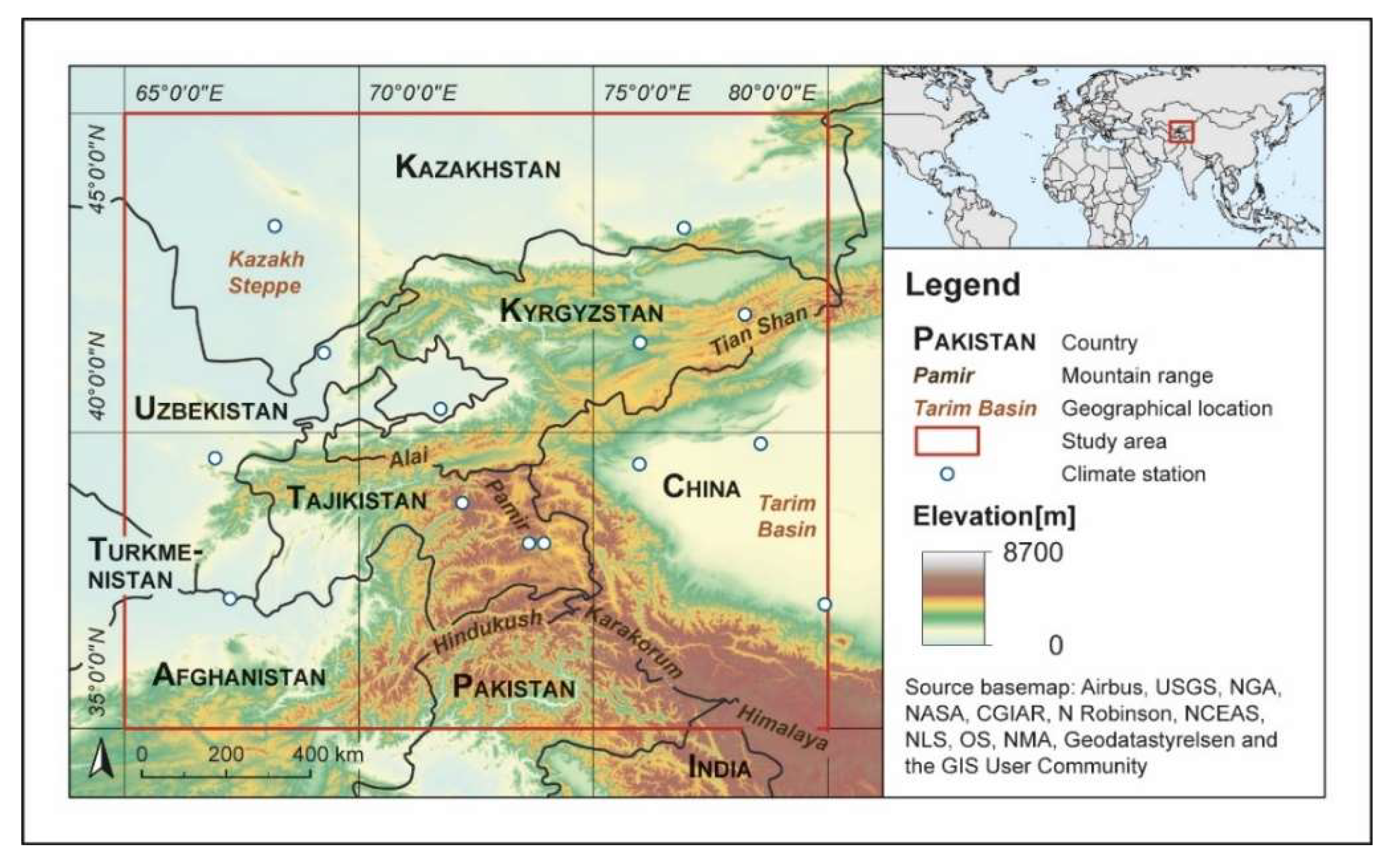
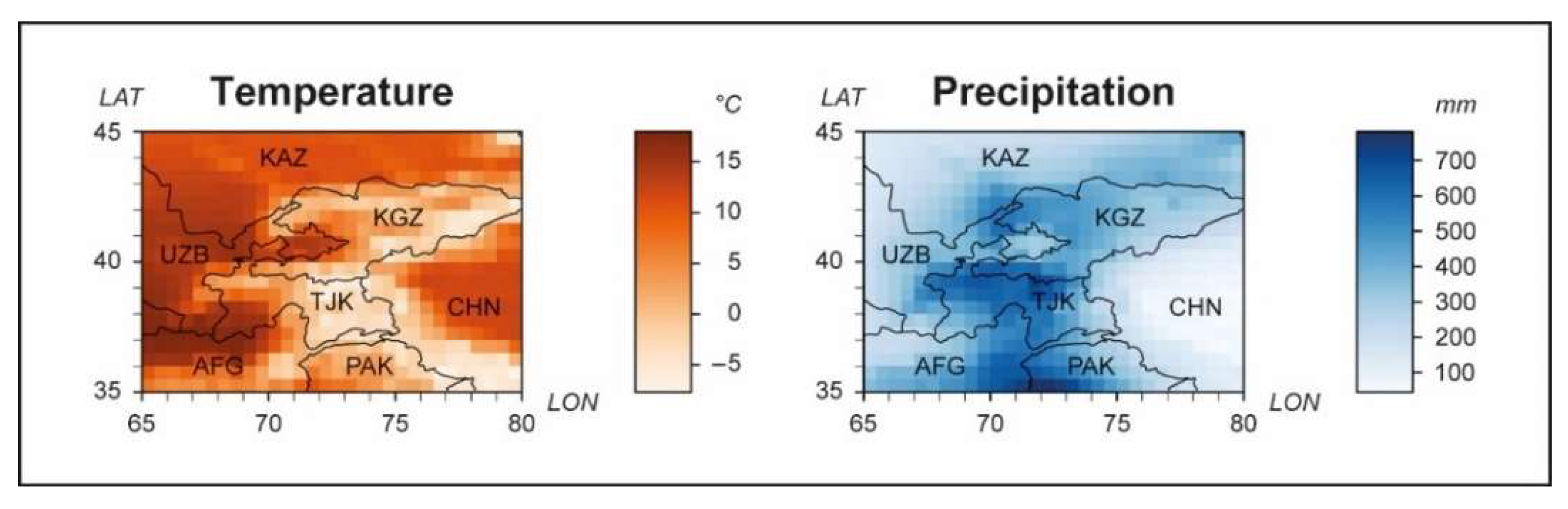
2.1. Study Area

The study area extends from 35°00’ to 45°00’ N and from 65°00’ to 80°00’ E and covers the territory of Tajikistan and Kyrgyzstan and the partly bordering areas of Turkmenistan, Uzbekistan, Kazakhstan, China, Pakistan, and Afghanistan (Figure 1). The area exhibits complex terrain, with high mountain systems in the east and southeast to lower, adjacent lowlands and basins in the northwest and west. Altitudinal differences range from under 100 masl in the northwest to up to 8000 masl in the southeast. Its continental location contributes towards arid-to-semiarid conditions and high seasonal variations. The climate of Central Asia is mainly controlled by the westerlies, the Central Asian High, and the Indian Monsoon [13,45,46]. The northern part of the research area is significantly dominated by the mid-latitude westerlies and cold inflows from polar regions [6,24,34,45]. The south is influenced by the Indian Monsoon, although its moisture level is largely reduced by the mountain ranges of the Hindukush, Pamir, and Himalaya. The strength and location of the Central Asian High determines the peak of annual precipitation to be in winter and spring, when humid cyclones from the Mediterranean region enter the region from the south/southwest [46,47]. However, due to its high continentality mean annual precipitation sums are generally low. Most precipitation falls, orographically induced, along the western and southern flanks of the mountain arc. From there on, they constantly decrease towards the east, reaching their minimum in the Tarim basin. Temperature on the other hand, shows its maxima in the eastern and western lowlands, and generally decreases with an altitudinal gradient (Figure 2).

2.2. Data

Table 1 gives an overview of the data sources used in this study. Whereas the CRU TS and the TRMM 3B43 have been used to conduct the trend analyses, the meteorological stations have been used to assess the local accuracy of the gridded products. The station requirements to be used for validation are (1) >80% of available data during 1950–2016 and (2) <5% missing values. Applying these criteria, no high altitude station is represented, which however would be important to validate the performance of the datasets over mountainous regions. Therefore, four stations above 2500 m have been additionally included, which do have at least a 50% data record coverage. The data is mostly complete for the period between 1950 and 1990. The location of the meteorological stations is shown in Figure 1.

2.2.1. CRU TS v. 4.01

To conduct the statistical analyses, the gridded dataset CRU TS v. 4.01 from the Climatic Research Unit at the University of East Anglia was used solely for temperature and in combination with TRMM 3B43 for precipitation. The CRU TS v. 4.01 was released in 2017 and is based on meteorological stations, providing interpolated data values on a 0.5° longitude/latitude grid. On average 33 and 46 stations were used between 1950–2016 for interpolating temperature and precipitation in the research area, respectively. The dataset contains ten different climatic variables, but only near-surface temperature and precipitation were used here. The dataset spans the period between 1901 and 2016. The monthly data were taken from January 1950 through December 2016. CRU TS v. 4.01 has been used in other regional climate change studies [5,34,49,50]. More information about the dataset and its influential stations can be found in [35]. To evaluate the performance of CRU we calculated the correlation coefficient after Kendall (R2), the root mean squared error (RMSE), and the mean absolute error (MAE) for the time period 1950–2016 (Table 2). The correlation and error calculation was undertaken by comparing the available station data with the corresponding grid cell of the dataset, where the station is located. CRU shows a high correlation with observational temperature records and comparatively low RMSE und MAE values. However, a slight overfitting is possible as some of the validation stations are very likely included in the original CRU dataset. In addition, insufficient data are available for the high-altitude stations.

2.2.2. TRMM 3B43 v.7

NASA’s Tropical Rainfall Measurement Mission version 3B43 V7 (TRMM 3B43) was used to provide information about recent decades’ precipitation sums in the research area. The TRMM 3B43 merges high-quality microwave data with infrared data and analysis of rain gauges and is, therefore, able to account for small-scale precipitation variability [38]. The processed product is provided at hourly resolution, gridded on a 0.25° longitude/latitude grid. The dataset spans the period from 1998 to current values. The data were obtained from January 1998 through December 2016. The TRMM 3B43 precipitation data has been used in validation studies and other global and regional precipitation analyses [40,51,52]. Before conducting the trend analysis, the hourly TRMM 3B43 data was accumulated into monthly sums. In order to match the resolution of CRU TS, the monthly TRMM 3B43 were spatially aggregated to the CRU TS spatial resolution. To evaluate the performance of TRMM 3B43 in the study area, we calculated the correlation coefficient after Kendall (R2), the root mean squared error (RMSE), and the mean absolute error (MAE) for the time period 1998–2016 (Table 2). Depending on the availability of station data, this time period could not always be fully covered. The performance measurements are undertaken by comparing the available station data with the corresponding grid cell of the dataset, where the station is located in. As many stations fell out of use after 1990, not every station remained suitable for validation. R2 shows strong differences between the stations, whereas positive values are highly significant. High-altitude stations do not provide any data during this time period.

2.3. Methods

All statistical analyses were completed using RStudio [53]. The graphics were finalized using ArcGIS (Esri Germany, Granzberg, Germany) and Adobe Illustrator (Adobe Systeme Software, Dublin, Ireland).

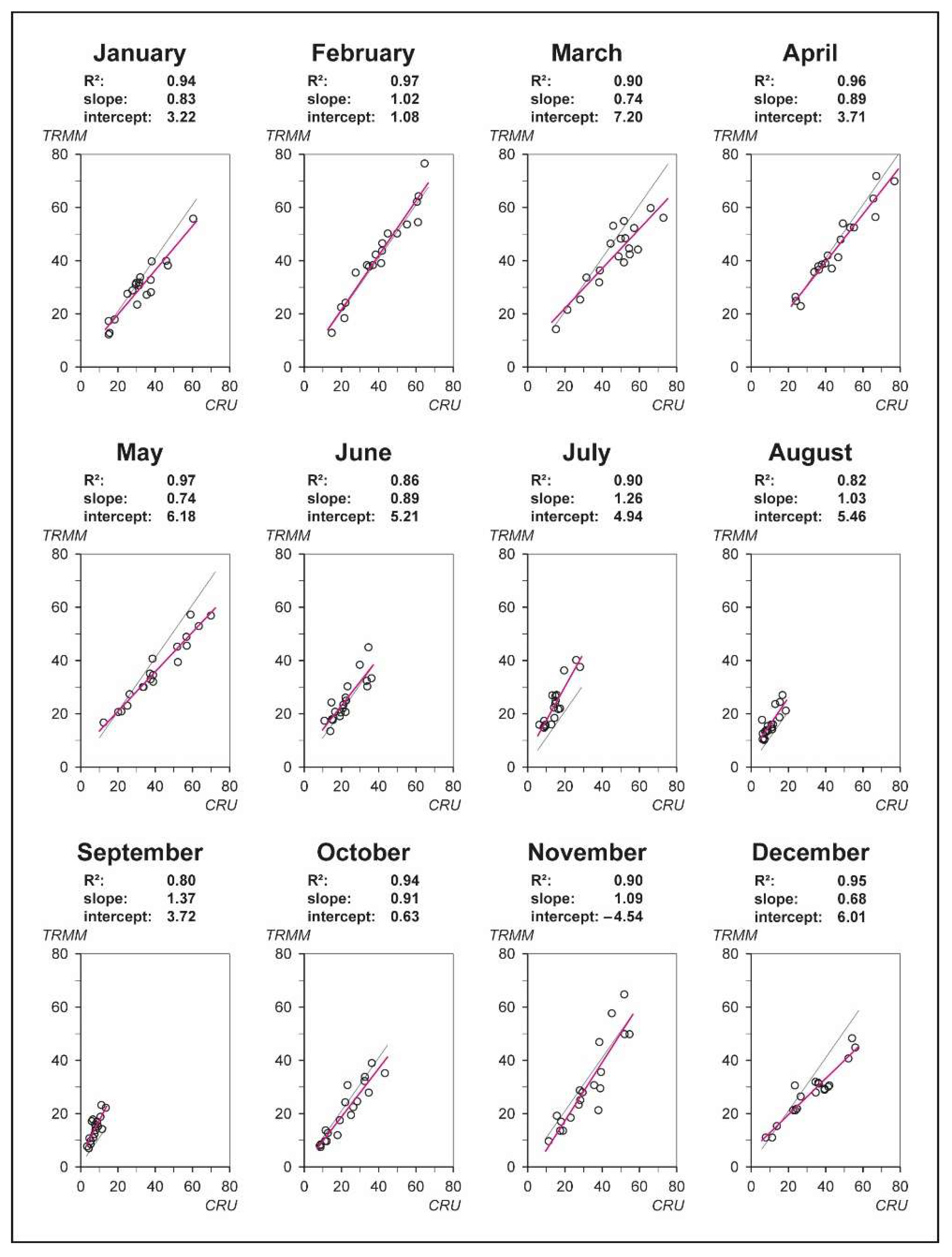
2.3.1. Linear Merging of the CRU TS and TRMM 3B43 Datasets

To conduct a long-term precipitation analysis, station-based gridded products are the only data source with a suitable temporal extent. However, high spatial variability of precipitation in combination with complex terrain and low meteorological station density reduced the accuracy of gridded, station-based precipitation products. Satellite-derived data has a much higher spatial resolution and is measured consistently over space, accounting for small-scale variability. Comparing CRU TS and TRMM 3B43 precipitation data for the period 1998–2016 shows a high correlation between the datasets, but differences in their monthly relationships (Figure 3). Looking at the different months, CRU TS mostly depicts higher values than TRMM 3B43, except for the summer months, where TRMM exceeds. To take the individual monthly amounts into account, we conducted a linear regression analysis between CRU TS and TRMM 3B43 on a monthly basis during their overlapping period 1998–2016. For each month, the estimated regression parameters were used to describe the statistical relationship between CRU TS and TRMM 3B43. To statistically adjust the historical CRU TS values according to this relationship, we calculated as follows:
Y i = α m +   X i ×   β m ,
where α is the intercept for month   m and β the slope for month m , with m ranging from 1–804. X i are the monthly CRU TS values from 1950–2016, with length i = 804 . The new dataset Y i was used to undertake the spatiotemporal precipitation analysis. The new dataset will be referred to as CRU TS/ TRMM 3B43. Table 2 shows the evaluation of CRU TS/TRMM 3B43 against observational records. Performance measurements were undertaken using the time period 1998–2016 to make the results comparable to the original TRMM performance. If the data availability of TRMM was not given during that period, 1950–2016 was chosen. Correlation values are lower than for temperature, but still high and significant. In comparison to the original TRMM performance, R2 strongly increased and RMSE and MAE decreased. This validation shows the improved performance of the new created CRU TS/TRMM 3B43 dataset, compared to TRMM 3B43.

2.3.2. Temporal Trend Analysis

Annual and seasonal climatic trends are computed by averaging the grid-cells in the region between 1950 and 2016. Seasons are defined as spring (MAM: March, April, May), summer (JJA: June, July, August), autumn (SON: September, October, November), and winter (DJF: December, January, February). Seasonal and annual anomaly time series were calculated in order to extract general trends and low-frequency (annual, decadal, multidecadal) variations. The anomalies were calculated by subtracting the seasonal temperature means for each year from its respective mean of the period 1950–2016. Furthermore, long-term linear trends and 10-year moving averages were separately applied to quantify the tendency of change and to smooth interannual variability, respectively. The significance of the trends is tested at the 95% confidence level. The moving average was calculated using the R-package ‘forecast’ [54]. In addition to the overall linear trend, a single change point detection has been applied using the R-package ‘cpm’ to find erratic changes in the mean of the data sequences [55].

2.3.3. Spatial Trend Analysis

Spatial changes in temperature and precipitation were analyzed using trend maps, showing the magnitude and significance of the derived linear trend, applied to every grid cell. Spatial differentiation between trends for higher elevation mountainous areas and lower elevation plains have been executed after the definition of the United Nations Environment Programme (UNEP). Mountain areas are defined as having (1) an elevation above 2500 m, (2) an elevation between 1500 m and 2500 m and a slope above 2°, (3) an elevation between 1000 m and 2500 m a slope above 5°, or (4) a local elevation above 300 m [56]. The significance and magnitude of the trends were derived using the function ‘pwmk’ from the R-package ‘modifiedmk’ [57]. The function ‘pwmk’, addresses the problem of temporal autocorrelation by prewhitening the time series prior to the trend calculation, following a similar approach to [58]. The trend magnitude is derived by Sen’s slope estimator and the trend significance using the Mann–Kendall test.

Mann–Kendall Test

The Mann–Kendall test is a non-parametric, rank-based test, to test the statistical significance of a monotonic trend [59,60]. The Mann–Kendall test determines the existence of a monotonic trend in the mean of the data and its significance. The test is suitable for climatological time series as it does not have any requirements of the joint distribution of the data, and is insensitive to outliers and missing values [61,62]. The Mann–Kendall test statistic S is estimated as follows:
S =   i = 1 n 1 s g n ( x i + 1 x i ) ,
where n is the length of the data set; xi+1 and xi are sequential data values. The test statistic S is then standardized by:
s g n ( Δ x ) =   { + 1 ,   Δ x > 0 0 ,   Δ x = 0 1 ,   Δ x < 0 ,
If S is positive, an increasing trend can be assessed in the data, whereas a negative S implies a decreasing trend. After [59] and [60] the test statistic S is approximately normally distributed if n 8 . In this case, the mean ( E ) and the variance ( V a r ) are calculated as follows:
E ( S ) = 0 ,
  V a r ( S ) = n ( n 1 ) ( 2 n + 5 ) i = 1 m t i ( t i 1 ) ( 2 t i + 5 ) 18 ,  
where m is the number of tied groups and ti is size of the ith group. The standardized test statistic Z is then computed with a mean of zero and a variance of one:
Z =   { S 1 V a r ( S ) , S > 0 S + 1 V a r ( S ) , S < 0 ,

Theil and Sen’s Slope Estimator

The Theil and Sen’s slope estimator specifies the magnitude of a trend [63,64]. Sen’s slope estimator was chosen over the widely used linear least square fitting method, as a normal distribution of the residuals is not always present in the climatological data. Sen’s slope estimator assesses the slope of n data pairs as follows:
Q = x t x t t t ,
where Q′ is the slope between the data points x_t’ and x_t; x_t’ is the data at time t and x_t is the data at time t. The slope of the data values is the median of the N values of Q values.
Sen’s slope estimator is simply given by:
Q = Q [ N + 1 2 ]   if   N   is   odd ,
  Q =   1 2 ( Q [ N + 1 2 ] + Q [ n + 2 2 ] )   i f   N   i s   e v e n  
where N is the number of calculated slopes.

3. Results

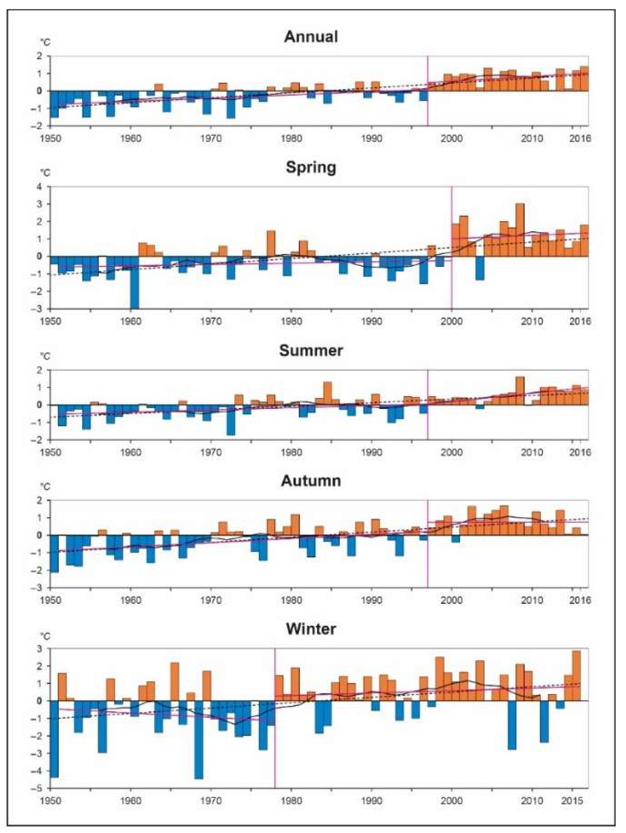
3.1. Temporal Changes in Air Temperature

Annual and seasonal mean surface temperatures increased significantly in the research area, showing a positive long-term trend, particularly in winter. Whereas annual temperatures increased at a rate of 0.28 °C per decade, the other seasonal trends lie in-between the minimum rate of 0.20 °C per decade in summer and the maximum rate of 0.32 °C per decade in winter (Table 3). However, the anomaly time series reveal the non-linear behavior of temperature change including prominent turning points in the seasonal averages (Figure 4). After the late-1990s the magnitude of the positive trend line gets accelerated in all seasons, except for winter. This warming period marks a turning point, from alternating warmer and colder years, towards a period of almost exceptionally strong positive deviations. In winter, the temperature change shows a different characteristic. Positive anomalies start to dominate in the late-1970s, inducing a longer, but less intense, time of warming.

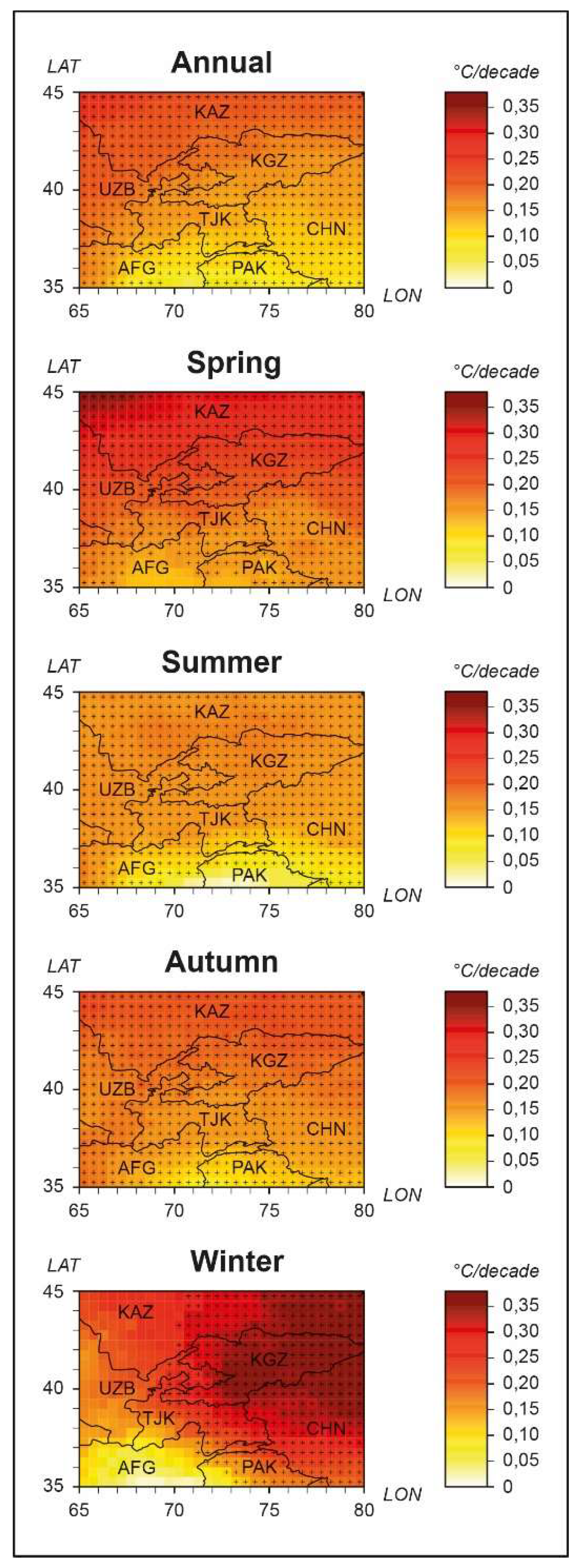
3.2. Spatial Changes in Air Temperature

Trend maps for 1950–2016 show the long-term magnitude and significance of linear temperature change per grid cell. The results, as shown in Figure 5, indicate a significant increase in temperature throughout the area. At the annual-mean scale, and in the spring, summer, and autumn seasons, the great majority of grid cells are significant at the 95% level, with the exception of the north of Afghanistan and Pakistan in summer and spring. In winter, a bipolar pattern of significantly higher warming rates in the east and non-significant lower warming rates in the west is visible. Regarding the intensity of the warming trend, northern regions are warming at a higher rate than southern regions (Figure 5). This north–south gradient is distinct in spring, summer, and autumn. In winter, a reducing temperature gradient from the northeast to the southwest is more pronounced. Elevation-based trend differences, according to our classification into ‘mountains’ and ‘plains’, are not distinct (Table 3). However, the lower plains show slightly higher trend rates than the mountainous region.

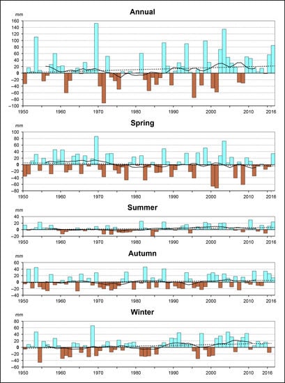
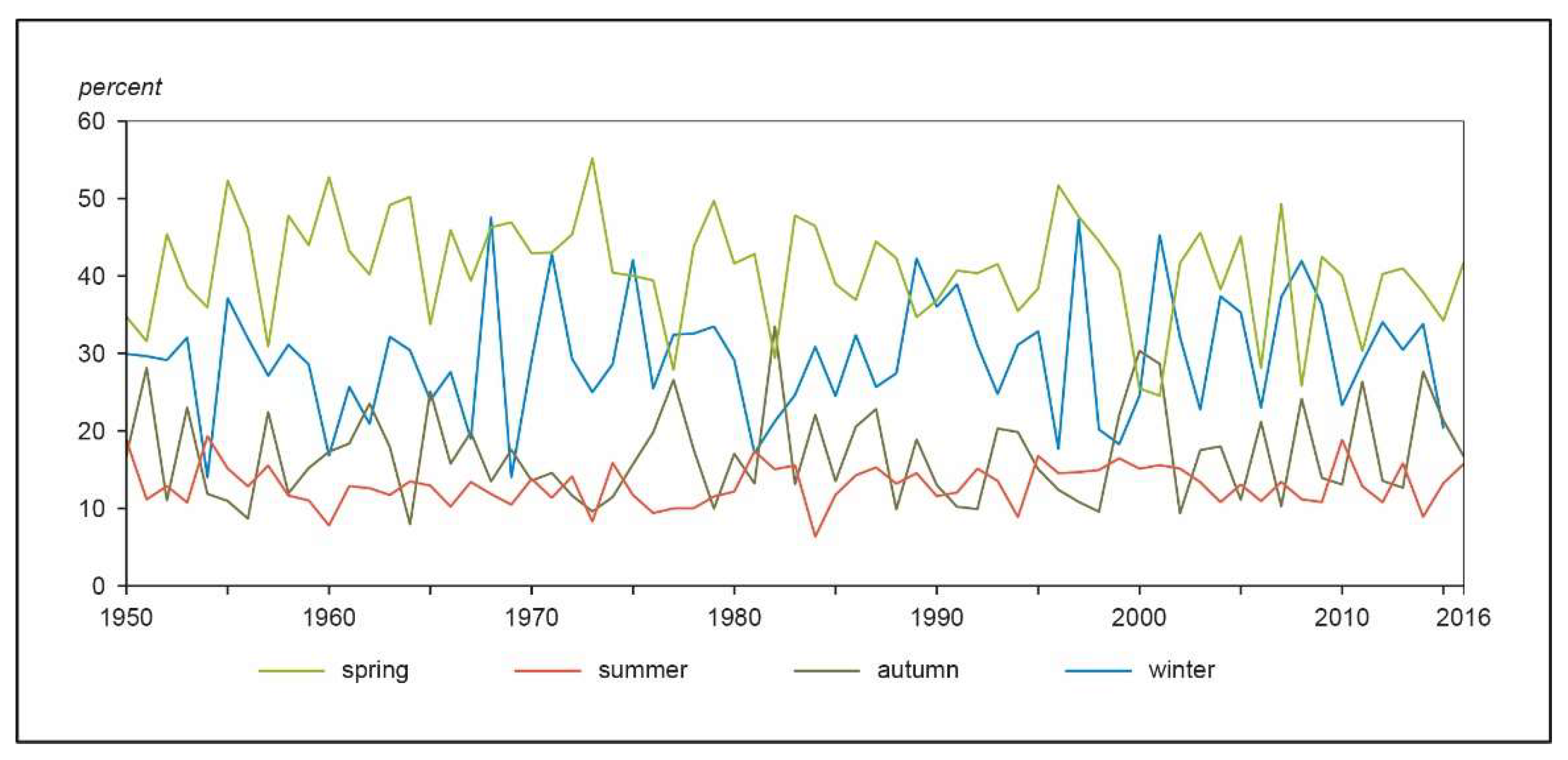
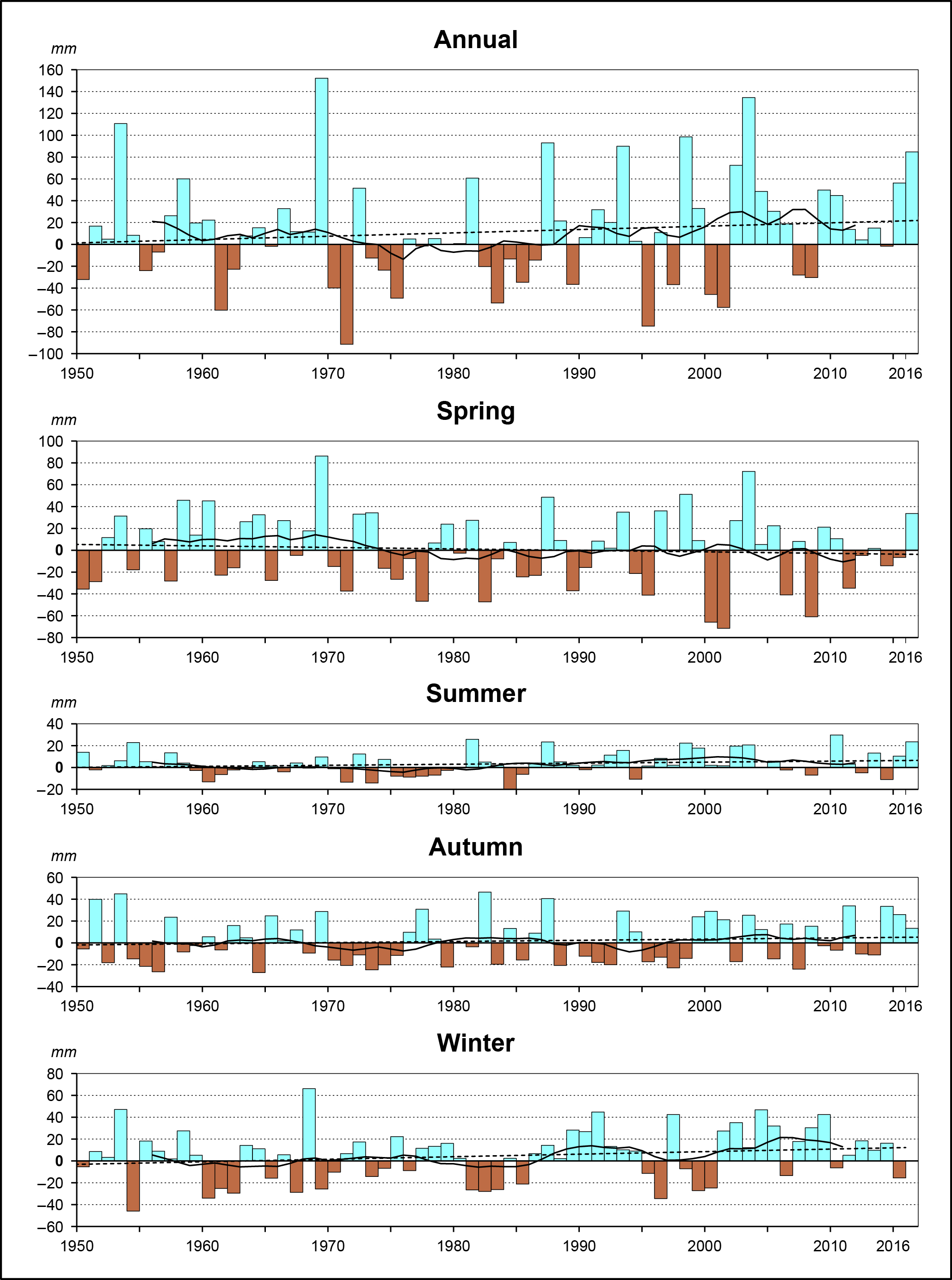
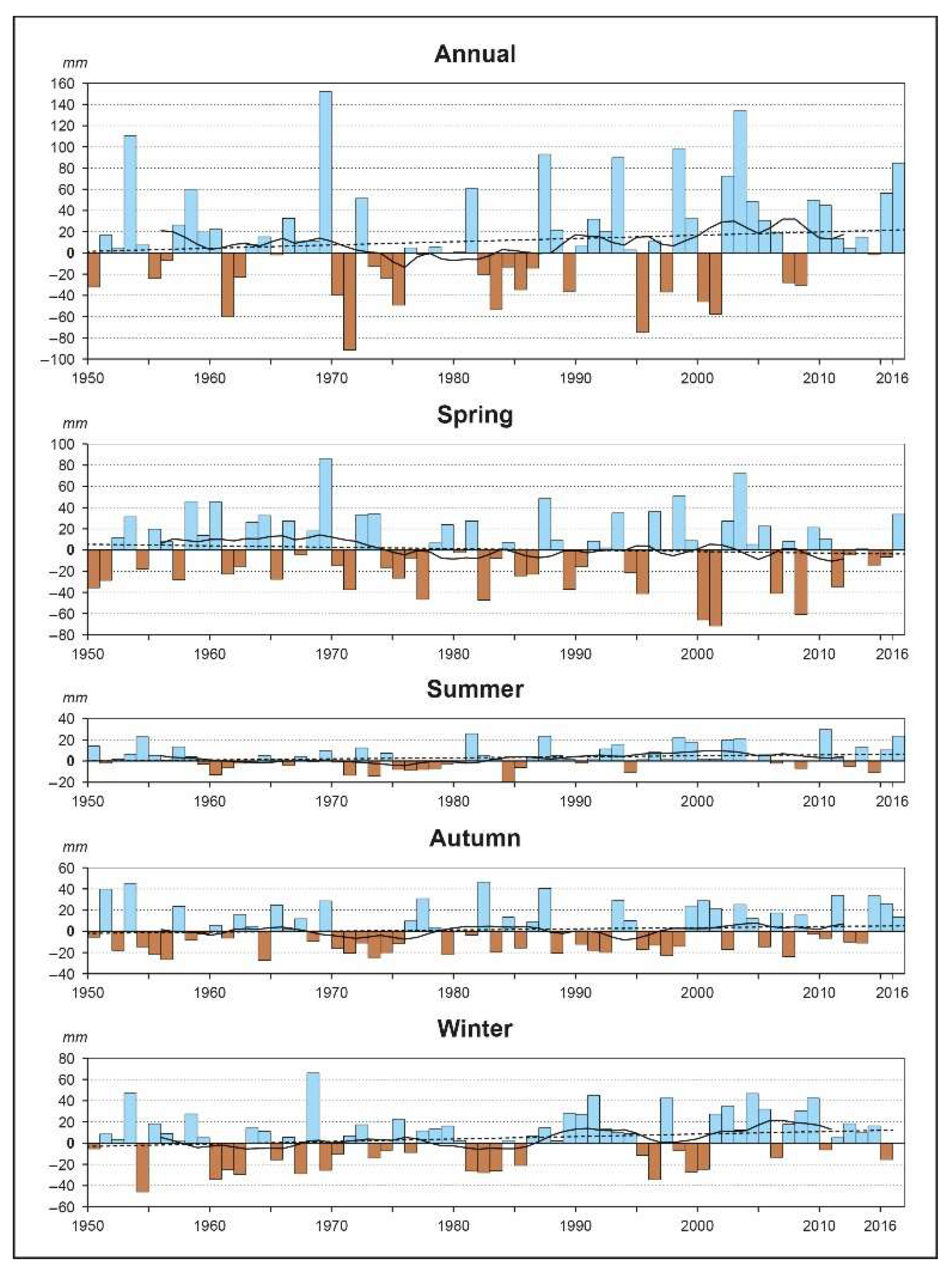
3.3. Temporal Changes in Precipitation

Annual and seasonal precipitation do not show any significant long-term statistical trend. Still, precipitation sums tend to increase at the annual level and in all seasons, except for spring. Annual precipitation increased by 3.13 mm per decade, mostly due to enhanced winter precipitation (Table 3). The anomaly time series reveal high year-to-year fluctuations within the seasons (Figure 6). In summer, autumn, and winter, a fluctuating pattern between consecutive years of either positive or negative anomalies is visible. In spring, anomalies alternate strongly at a yearly basis, with additional growth of the recent years’ negative deviations. Considering the proportions of seasonal precipitation over time, no profound change can be detected. The highest proportion of annual precipitation occurs in spring (40%), followed by winter (29%). In these two seasons, which provide over two-thirds of the annual precipitation, the variability within the data is much higher than in the dry summer months, where precipitation is the lowest of all four seasons (13%) (Figure 7).

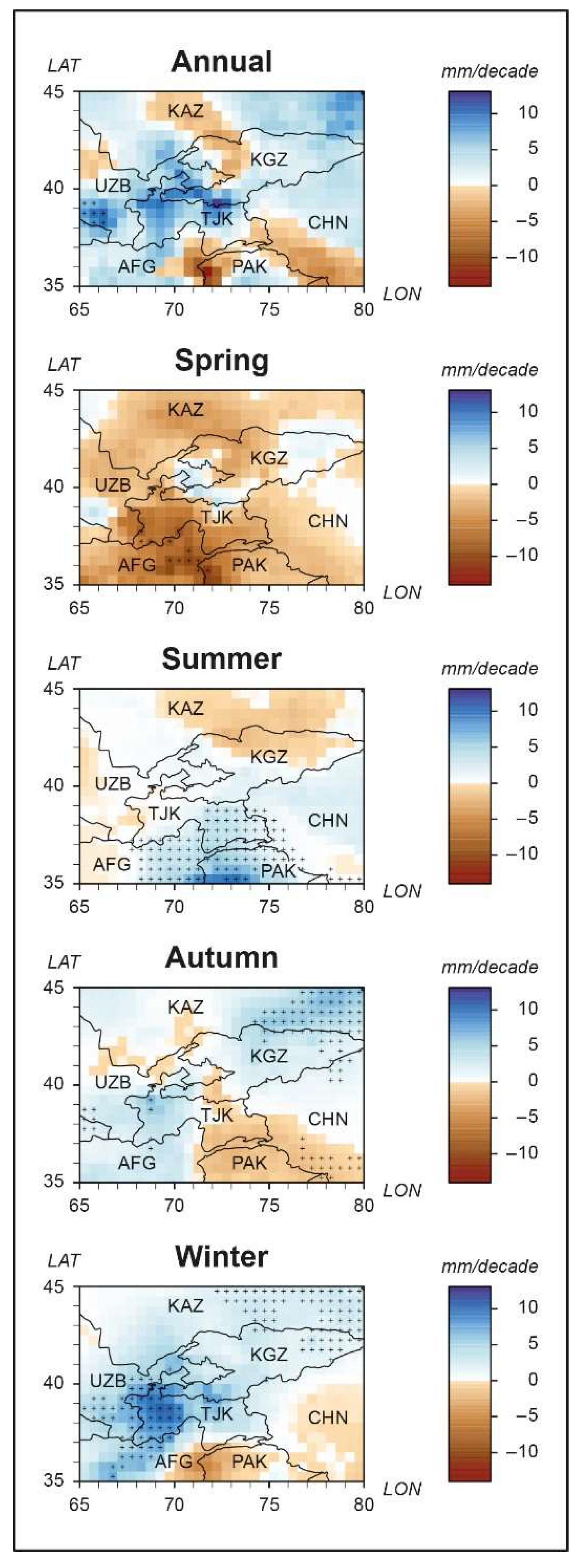
3.4. Spatial Changes in Precipitation

In the great majority of the research area, precipitation is not changing significantly (Figure 8). However, the summer, autumn, and winter seasons exhibit isolated patches of significant changes. In summer, the north of Afghanistan and Pakistan, and the Tajik Pamirs are significantly gaining precipitation. In winter, significantly increasing trends can be seen around West Tajikistan and in the northeastern corner of the research area. The intensity of precipitation trends is also unevenly distinct but, often, high trends coincide with the identified significance areas (Figure 8). The largest region of decreasing precipitation trends occurs in spring, covering almost the whole research area. In winter and autumn, drier regions are narrowed down towards the southeast quarter of the research area, whereas in summer, less precipitation can be observed in the region along the northern border of Kyrgyzstan. One of the most pronounced areas of precipitation are located in the north of Afghanistan and Pakistan, and in the Tajik Pamirs in summer. In autumn and winter, a diagonal zone from the southwest to the northeast displays positive trends. In both seasons, additional enhanced spots can be seen in the northeast corner of the research area and West Tajikistan, respectively. Whereas the trend maps do not reveal a clear distinction between different trend tendencies in mountainous and plain regions, Table 3 outlines a stronger increase in precipitation for the lower plains. However, this is not significant.

4. Discussion

Our study confirms the strong warming trend of Central Asia, with an abrupt acceleration of its intensity in the mid-1990s. The significant increase in annual and seasonal temperatures has already been identified in previous studies, however with different trend magnitudes [3,24,25]. Our results indicated an annual temperature increase of 0.28 °C per decade (1950–2016), compared to the outcomes of [3] and [24], who found an annual temperature increase of 0.39 °C per decade (1979–2011) and 0.16 °C per decade (1901–2003), respectively. Discrepancies in the trend magnitudes are likely caused by different regional extents, time periods, and data sources. This methodological constraint might also affect the results of other Central Asian studies [3,5,65,66], and global studies [67], as their time series also show an abrupt change of the mean in the late 20th century. It can be summarized that, despite different time periods and different datasets, all large-scale studies agreed on a strong warming trend averaged over Central Asia, which has accelerated in recent years.
Seasonal investigations in trend characteristics showed that spring and winter are under the greatest change. Spring and winter are important seasons in Central Asian because (1) two thirds of the annual precipitation is falling during that time, and (2) water reservoirs in the form of snow and ice are built up [68]. Altered precipitation patterns during these months can induce water shortages in summer, effect agricultural yields in autumn, and modify snow-regimes [9,69,70]. However, our data does not reveal any significant changes in precipitation. In terms of temperature, both seasons show a significant increase. According to our results, winter displays the highest rate of temperature increase (0.32 °C per decade), followed by spring. These data are consistent with earlier studies that also show winter as the most rapidly warming season in this region [13,18,24]. Some studies, however, show the contrary, with spring as the greatest warming season, directly followed by winter [3]. According to [49], it can be summarized that the colder seasons of the year are warming the most in semi-arid regions.
As temporal trends are averaged over the whole research area, it is important to assess their local characteristics by using grid-based trend maps. The accuracy of the trend maps is defined by the spatial resolution of the input data. Therefore, to reveal spatial trend differences the choice of data is important. Our data has a resolution of 0.5 degree and can account for general differences between geographical regions (Figure 4 and Figure 7). Using this data we identified a general increase in temperature across the whole research area, whereas the northern parts do warm more than the southern parts. Finding a possible explanation for this north–south gradient was beyond the scope of this study and should be further investigated in future research. In terms of precipitation no clear pattern could be identified using the visual trend maps. However, as earlier studies already assessed the importance of elevation dependent temperature and precipitation rates [71] but gained controversial results, we looked at this in more detail, calculating additional trend rates. Due to the scarce coverage of meteorological stations in high-altitude areas, it is difficult to gain significant evidence for elevation dependent gradients. Therefore, earlier study results are often contradicting. Whereas [19] does not recognize altitudinal effects on temperature change, [3] found that lower elevations warm more than higher elevations, but only in some regions in Central Asia. For precipitation it is even more difficult, as it can be spatially and temporally highly variable. However, both [17,29] detected a slight tendency towards higher trend rates in lower Central Asian plains. Our results also show higher trend magnitudes for plains, but not at a significant level (Table 3). The same situation can be seen for temperature, where plains tend to increase at a stronger rate. These results might be affected by the lack of observational data in high-elevation areas. In addition, looking at the spatial distribution of temperature and precipitation trends in Figure 5 and Figure 8, no clear difference between trend tendencies in plains and mountains can be seen. As the mountains of Central Asia are inhabited at many different altitudinal levels and because the impacts of climate change can have different characteristics from valley to valley, it is important to build up the station network to higher altitudes. This would allow to obtain more precise information about elevation-dependent trends and impacts, especially because communities at high-altitudes are less resilient against climatic changes, as their food and water sources are limited.
The accuracy of the results is limited by the availability of accurate climate data in high altitudes and missing long-term records. The complexity of the terrain makes regional trends differ greatly from large-scale observations and the sparse meteorological stations coverage impacts the accuracy of Central Asian gridded climate datasets. Due to the low resolution of the applied gridded products, climatic processes at finer spatial and temporal scales, like extreme events or low-frequency variations are neglected [72,73]. To obtain information about fine-scale processes, which are important for assessing climate change impacts and vulnerability scenarios, various downscaling methods or stochastic models could be applied [72,73,74]. By applying a combined dataset of the gridded station product CRU TS and the satellite product TRMM 3B43, we attempted to account for the problem of precipitation data accuracy. Nevertheless, our trend magnitudes differed from previous studies, whereas the general tendency was in accordance. It is a challenge to analyze precipitation trends in complex and data sparse regions. However, understanding climatic change in Central Asia and investigating its regional differences is important because of the subsistence-based and natural-controlled lifestyle of the rural communities and the dependence on glacier and snow packs for the regional water supply. To provide a suitable basis for adaptation strategies, 0.5 degree resolution is insufficient in a complex mountainous terrain. Therefore, future studies should amplify their spatial resolution and focusing on the level on the villages, because that is the level where people are impacted by the consequences of climate change.

Author Contributions

Conceptualization: I.H., P.D.J., and C.S.; formal analysis: I.H.; investigation: I.H.; methodology: I.H., P.D.J., and C.S.; supervision: I.H., P.D.J., and C.S.; validation: I.H.; visualization: I.H.; writing—original draft: I.H.; writing—review and editing: I.H., P.D.J., and C.S.

Funding

This research was funded by the Belmont Forum and Deutsche Forschungsgemeinschaft, project number SA 775/12-1 and the University of Bayreuth in the funding programme Open Access Publishing.

Conflicts of Interest

The authors declare no conflict of interest.

References

  1. Giorgi, F. Climate change hot-spots. Geophys. Res. Lett. 2006, 33. [Google Scholar] [CrossRef]
  2. De Beurs, K.M.; Henebry, G.M.; Owsley, B.C.; Sokolik, I.N. Large scale climate oscillation impacts on temperature, precipitation and land surface phenology in Central Asia. Environ. Res. Lett. 2018, 13, 65018. [Google Scholar] [CrossRef]
  3. Hu, Z.; Zhang, C.; Hu, Q.; Tian, H. Temperature changes in Central Asia from 1979 to 2011 based on multiple datasets. J. Clim. 2014, 27, 1143–1167. [Google Scholar] [CrossRef]
  4. Zhang, M.; Chen, Y.; Shen, Y.; Li, B. Tracking climate change in Central Asia through temperature and precipitation extremes. J. Geogr. Sci. 2019, 29, 3–28. [Google Scholar] [CrossRef] [Green Version]
  5. Chen, F.; Huang, W.; Jin, L.; Chen, J.; Wang, J. Spatiotemporal precipitation variations in the arid Central Asia in the context of global warming. Sci. China Earth Sci. 2011, 54, 1812–1821. [Google Scholar] [CrossRef]
  6. Hu, Z.; Zhou, Q.; Chen, X.; Qian, C.; Wang, S.; Li, J. Variations and changes of annual precipitation in Central Asia over the last century. Int. J. Climatol. 2017, 37, 157–170. [Google Scholar] [CrossRef]
  7. Reyer, C.P.O.; Otto, I.M.; Adams, S.; Albrecht, T.; Baarsch, F.; Cartsburg, M.; Coumou, D.; Eden, A.; Ludi, E.; Marcus, R.; et al. Climate change impacts in Central Asia and their implications for development. Reg. Environ. Chang. 2015. [Google Scholar] [CrossRef]
  8. Seim, A.; Schultz, J.A.; Leland, C.; Davi, N.; Byambasuren, O.; Liang, E.; Wang, X.; Beck, C.; Linderholm, H.W.; Pederson, N. Synoptic-scale circulation patterns during summer derived from tree rings in mid-latitude Asia. Clim. Dyn. 2016, 49, 1917–1931. [Google Scholar] [CrossRef] [Green Version]
  9. Siegfried, T.; Bernauer, T.; Guiennet, R.; Sellars, S.; Robertson, A.W.; Mankin, J.; Bauer-Gottwein, P.; Yakovlev, A. Will climate change exacerbate water stress in Central Asia? Clim. Chang. 2012, 112, 881–899. [Google Scholar] [CrossRef]
  10. Yin, G.; Hu, Z.; Chen, X.; Tiyip, T. Vegetation dynamics and its response to climate change in Central Asia. J. Arid Land 2016, 8, 375–388. [Google Scholar] [CrossRef] [Green Version]
  11. Xenarios, S.; Gafurov, A.; Schmidt-Vogt, D.; Sehring, J.; Manandhar, S.; Hergarten, C.; Shigaeva, J.; Foggin, M. Climate change and adaptation of mountain societies in Central Asia: Uncertainties, knowledge gaps, and data constraints. Reg. Environ. Change 2019, 19, 1339–1352. [Google Scholar] [CrossRef]
  12. Hijioka, Y.; Lin, E.; Pereira, J.J.; Corlett, R.T.; Gui, X.; Insarov, G.E.; Lasco, R.D.; Lindgren, E.; Surjan, A. Asia. In Climate Change 2014: Impacrs, Adaptation, and Vulnerability. Part B: Regional Aspects. Contributions of Working Group II to the Fith Assessment Report of the Intergovernmental Panel on Climate Change; Barros, V.R., Field, C.B., Dokken, D.J., Mastrandrea, M.D., Mach, K.J., Bilir, T.E., Chatterjee, M., Ebi, K.L., Estrada, Y.O., Genova, R.C., et al., Eds.; Cambridge University Press: Cambridge, UK; New York, NY, USA, 2014. [Google Scholar]
  13. Lioubimtseva, E.; Henebry, G.M. Climate and environmental change in arid Central Asia: Impacts, vulnerability, and adaptations. J. Arid Environ. 2009, 73, 963–977. [Google Scholar] [CrossRef]
  14. Bhutiyani, M.R.; Kale, V.S.; Pawar, N.J. Climate change and the precipitation variations in the northwestern Himalaya: 1866–2006. Int. J. Climatol. 2010, 85. [Google Scholar] [CrossRef]
  15. Liu, X.; Chen, B. Climatic warming in the Tibetan Plateau during recent decades. Int. J. Climatol. 2000, 20, 1729–1742. [Google Scholar] [CrossRef]
  16. Shekhar, M.S.; Chand, H.; Kumar, S.; Srinivasan, K.; Ganju, A. Climate-change studies in the western Himalaya. Ann. Glaciol. 2010, 51, 105–112. [Google Scholar] [CrossRef] [Green Version]
  17. Bolch, T. Climate change and glacier retreat in northern Tien Shan (Kazakhstan/Kyrgyzstan) using remote sensing data. Glob. Planet. Chang. 2007, 56, 1–12. [Google Scholar] [CrossRef]
  18. Hu, Z.; Li, Q.; Chen, X.; Teng, Z.; Chen, C.; Yin, G.; Zhang, Y. Climate changes in temperature and precipitation extremes in an alpine grassland of Central Asia. Theor. Appl. Climatol. 2016, 126, 519–531. [Google Scholar] [CrossRef]
  19. Xu, M.; Kang, S.; Wu, H.; Yuan, X. Detection of spatio-temporal variability of air temperature and precipitation based on long-term meteorological station observations over Tianshan Mountains, Central Asia. Atmos. Res. 2018, 203, 141–163. [Google Scholar] [CrossRef]
  20. Hartmann, H.; Buchanan, H. Trends in extreme precipitation events in the Indus river basin and flooding in Pakistan. Atmos. Ocean 2014, 52, 77–91. [Google Scholar] [CrossRef]
  21. Palazzi, E.; von Hardenberg, J.; Provenzale, A. Precipitation in the Hindu-Kush Karakoram Himalaya: Observations and future scenarios. J. Geophys. Res. Atmos. 2013, 118, 85–100. [Google Scholar] [CrossRef]
  22. Ren, Y.-Y.; Ren, G.-Y.; Sun, X.-B.; Shrestha, A.B.; You, Q.-L.; Zhan, Y.-J.; Rajbhandari, R.; Zhang, P.-F.; Wen, K.-M. Observed changes in surface air temperature and precipitation in the Hindu Kush Himalayan region over the last 100-plus years. Adv. Clim. Change Res. 2017, 8, 148–156. [Google Scholar] [CrossRef]
  23. Immerzeel, W.W.; van Beck, L.P.H.; Bierkens, M.F.P. Climate change will affect the Asian water towers. Science 2010, 328, 1382–1385. [Google Scholar] [CrossRef] [PubMed]
  24. Chen, F.; Wang, J.; Jin, L.; Zhang, Q.; Li, J.; Chen, J. Rapid warming in mid-latitude central Asia for the past 100 years. Front. Earth Sci. China 2009, 3, 42–50. [Google Scholar] [CrossRef]
  25. Chen, Z.; Chen, Y.; Bai, L.; Xu, J. Multiscale evolution of surface air temperature in the arid region of Northwest China and its linkages to ocean oscillations. Theor. Appl. Climatol. 2017, 128, 945–958. [Google Scholar] [CrossRef]
  26. Feng, R.; Yu, R.; Zheng, H.; Gan, M. Spatial and temporal variations in extreme temperature in Central Asia. Int. J. Climatol. 2018, 38, e388–e400. [Google Scholar] [CrossRef]
  27. Aizen, E.M.; Aizen, V.B.; Melack, J.M.; Nakamura, T.; Ohta, T. Precipitation and atmospheric circulation patterns at mid-latitudes of Asia. Int. J. Climatol. 2001, 21, 535–556. [Google Scholar] [CrossRef]
  28. Song, S.; Bai, J. Increasing winter precipitation over arid Central Asia under global warming. Atmosphere 2016, 7, 139. [Google Scholar] [CrossRef]
  29. Chen, X.; Wang, S.; Hu, Z.; Zhou, Q.; Hu, Q. Spatiotemporal characteristics of seasonal precipitation and their relationships with ENSO in Central Asia during 1901–2013. J. Geogr. Sci. 2018, 28, 1341–1368. [Google Scholar] [CrossRef]
  30. Klein Tank, A.M.G.; Peterson, T.C.; Quadir, D.A.; Dorji, S.; Zou, X.; Tang, H.; Santhosh, K.; Joshi, U.R.; Jaswal, A.K.; Kolli, R.K.; et al. Changes in daily temperature and precipitation extremes in Central and South Asia. J. Geophys. Res. 2006, 111, D23107. [Google Scholar] [CrossRef]
  31. Yao, J.; Chen, Y. Trend analysis of temperature and precipitation in the Syr Darya Basin in Central Asia. Theor. Appl. Climatol. 2015, 120, 521–531. [Google Scholar] [CrossRef]
  32. Hu, Z.; Hu, Q.; Zhang, C.; Chen, X.; Li, Q. Evaluation of reanalysis, spatially interpolated and satellite remotely sensed precipitation data sets in central Asia. J. Geophys. Res. Atmos. 2016, 121, 5648–5663. [Google Scholar] [CrossRef] [Green Version]
  33. Pohl, E.; Knoche, M.; Gloaguen, R.; Andermann, C.; Krause, P. The hydrological cycle in the high Pamir Mountains: How temperature and seasonal precipitation distribution influence stream flow in the Gunt catchment, Tajikistan. Earth Surf. Dynam. Discuss. 2014, 2, 1155–1215. [Google Scholar] [CrossRef]
  34. Schiemann, R.; Lüthi, D.; Vidale, P.L.; Schär, C. The precipitation climate of Central Asia—Intercomparison of observational and numerical data sources in a remote semiarid region. Int. J. Climatol. 2008, 28, 295–314. [Google Scholar] [CrossRef]
  35. Harris, I.; Jones, P.D.; Osborn, T.J.; Lister, D.H. Updated high-resolution grids of monthly climatic observations—The CRU TS3.10 Dataset. Int. J. Climatol. 2014, 34, 623–642. [Google Scholar] [CrossRef]
  36. Schamm, K.; Ziese, M.; Raykova, K.; Becker, A.; Finger, P.; Meyer-Christoffer, A.; Schneider, U. GPCC Full Data Daily Version 1.0 at 1.0: Daily Land-Surface Precipitation from Rain-Gauges built on GTS-based and Historic Data. Archive at the National Center for Atmospheric Research, Computational and Information Systems Laboratory. Available online: https://doi.org/10.5065/D6V69GRT (accessed on 1 March 2017).
  37. Willmott, C.J.; Matsuura, K. Terrestrial Air Temperature: 1900–2010 Gridded Monthly Time Series (1900–2010): Version 3.01. Available online: http://climate.geog.udel.edu/~climate/html_pages/README.ghcn_ts2.html (accessed on 1 March 2018).
  38. Huffman, G.J.; Bolvin, D.T.; Nelkin, E.J.; Wolff, D.B.; Adler, R.F.; Gu, G.; Hong, Y.; Bowman, K.P.; Stocker, E.F. The TRMM multisatellite precipitation analysis (TMPA): Quasi-Global, multiyear, combined-sensor precipitation estimates at fine scales. J. Hydrometeorol. 2007, 8, 38–55. [Google Scholar] [CrossRef]
  39. Tropical Rainfall Measuring Mission (TRMM). TRMM 2011 (TMPA/3B43) Rainfall Estimate L3 1 Month 0.25 Degree × 0.25 Degree V7, Greenbelt, MD, Goddard Earth Sciences Data and Information Services Center (GES DISC). Available online: https://disc.gsfc.nasa.gov/datacollection/TRMM_3B43_7.html (accessed on 1 March 2018).
  40. Karaseva, M.O.; Prakash, S.; Gairola, R.M. Validation of high-resolution TRMM-3B43 precipitation product using rain gauge measurements over Kyrgyzstan. Theor. Appl. Climatol. 2012, 108, 147–157. [Google Scholar] [CrossRef]
  41. Rana, S.; McGregor, J.; Renwick, J. Wintertime precipitation climatology and ENSO sensitivity over central southwest Asia. Int. J. Climatol. 2017, 37, 1494–1509. [Google Scholar] [CrossRef]
  42. Yang, Y.; Luo, Y. Evaluating the performance of remote sensing precipitation products CMORPH, PERSIANN, and TMPA, in the arid region of northwest China. Theor. Appl. Climatol. 2014, 118, 429–445. [Google Scholar] [CrossRef]
  43. Guo, H.; Chen, S.; Bao, A.; Hu, J.; Gebregiorgis, A.; Xue, X.; Zhang, X. Inter-Comparison of high-resolution satellite precipitation products over Central Asia. Remote Sens. 2015, 7, 7181–7211. [Google Scholar] [CrossRef]
  44. Zhao, W.; Yu, X.; Ma, H.; Zhu, Q.; Zhang, Y.; Qin, W.; Ai, N.; Wang, Y. Analysis of precipitation characteristics during 1957–2012 in the Semi-Arid Loess Plateau, China. PLoS ONE 2015, 10, 1–13. [Google Scholar] [CrossRef]
  45. Huang, A.; Zhou, Y.; Zhang, Y.; Huang, D.; Zhao, Y.; Wu, H. Changes of the annual precipitation over Central Asia in the twenty-first century projected by multimodels of CMIP5. J. Clim. 2014, 27, 6627–6646. [Google Scholar] [CrossRef]
  46. Small, E.E.; Giorgi, F.; Sloan, L.C. Regional climate model simulation of precipitation in central Asia: Mean and interannual variability. J. Geophys. Res. 1999, 104, 6563–6582. [Google Scholar] [CrossRef]
  47. Böhner, J. General climatic controls and topoclimatic variations in Central and High Asia. Boreas 2006, 35, 279–295. [Google Scholar] [CrossRef]
  48. National Centers for Environmental Information (NCEI). Climate Data Online (CDO)—The National Climatic Data Center’s (NCDC) Climate Data Online (CDO) Provides Free Access to NCDC’s Archive of Historical Weather and Climate Data in Addition to Station History Information. National Climatic Data Center (NCDC). Available online: https://www.ncdc.noaa.gov/cdo-web/ (accessed on 22 August 2019).
  49. Huang, J.; Guan, X.; Ji, F. Enhanced cold-season warming in semi-arid regions. Atmos. Chem. Phys. 2012, 12, 5391–5398. [Google Scholar] [CrossRef] [Green Version]
  50. Zhao, Y.; Zhang, H. Impacts of SST warming in tropical Indian Ocean on CMIP5 model-projected summer rainfall changes over Central Asia. Clim. Dyn. 2016, 46, 3223–3238. [Google Scholar] [CrossRef]
  51. Mao, J.; Wu, G. Diurnal variations of summer precipitation over the Asian monsoon region as revealed by TRMM satellite data. Sci. China Earth Sci. 2012, 55, 554–566. [Google Scholar] [CrossRef]
  52. Shrestha, D.; Singh, P.; Nakamura, K. Spatiotemporal variation of rainfall over the central Himalayan region revealed by TRMM precipitation radar. J. Geophys. Res. 2012, 117. [Google Scholar] [CrossRef]
  53. RStudio: Integrated Development Environment for R; RStudio, Inc.: Boston, MA, USA, 2012.
  54. Hyndman, R.J.; Athanasopoulos, G.; Bergmeir, C.; Caceres, G.; Chhay, L.; O’Hara-Wild, M.; Petropoulos, F.; Razbash, S.; Wang, E.; Yasmeen, F. Forecast: Forecasting functions for time series and linear models. R package. 2019. [Google Scholar]
  55. Ross, G.J. Parametric and nonparametric sequential change detection in R: The cpm package. J. Stat. Softw. 2015, 66. [Google Scholar] [CrossRef]
  56. Blyth, S.; Groombridge, B.; Lysenko, I.; Miles, L.; Newton, A. Mountain Watch; Cambridge University Press: Cambridge, UK, 2002. [Google Scholar]
  57. Patakamuri, S.K. Modifiedmk: Modified Mann Kendall Trend Tests. R package version. 2017. [Google Scholar]
  58. Yue, S.; Wang, C.Y. Applicability of prewhitening to eliminate the influence of serial correlation on the Mann–Kendall test. Water Resour. Res. 2002, 38, 41–47. [Google Scholar] [CrossRef]
  59. Mann, H.B. Nonparametric tests against trend. Econometrica 1945, 13, 245–259. [Google Scholar] [CrossRef]
  60. Kendall, M. Rank Correlation Methods; Charles Griffin & Company LTD: London/High Wycombe, UK, 1975. [Google Scholar]
  61. Blain, G.C. Removing the influence of the serial correlation on the Mann–Kendall test. Rev. Bras. Meteorol. 2014, 29, 161–170. [Google Scholar] [CrossRef]
  62. Yue, S.; Pilon, P.; Phinney, B.; Cavadias, G. The influence of autocorrelation on the ability to detect trend in hydrological series. Hydrol. Process. 2002, 16, 1807–1829. [Google Scholar] [CrossRef]
  63. Sen, P.K. Estimates of the regression coefficient based on Kendall’s tau. Ј. Am. Stat. Assoc. 1968, 63, 1379–1389. [Google Scholar] [CrossRef]
  64. Theil, H. A rank-invariant method of linear and polynomial regression analysis. Part 3. Ned. Akad. Wet. 1950, 53, 1397–1412. [Google Scholar]
  65. Bhutiyani, M.R.; Kale, V.S.; Pawar, N.J. Long-term trends in maximum, minimum and mean annual air temperatures across the Northwestern Himalaya during the twentieth century. Clim. Change 2007, 85, 159–177. [Google Scholar] [CrossRef]
  66. Geng, Q.; Wu, P.; Zhao, X. Spatial and temporal trends in climatic variables in arid areas of northwest China. Int. J. Climatol. 2016, 36, 4118–4129. [Google Scholar] [CrossRef]
  67. Jones, P.D.; Harpham, C.; Harris, I.; Goodess, C.M.; Burton, A.; Centella-Artola, A.; Taylor, M.A.; Bezanilla-Morlot, A.; Campbell, J.D.; Stephenson, T.S.; et al. Long-term trends in precipitation and temperature across the Caribbean. Int. J. Climatol. 2016, 36, 3314–3333. [Google Scholar] [CrossRef]
  68. Syed, F.S.; Giorgi, F.; Pal, J.S.; Keay, K. Regional climate model simulation of winter climate over Central-Southwest Asia, with emphasis on NAO and ENSO effects. Int. J. Climatol. 2010, 30, 220–235. [Google Scholar] [CrossRef]
  69. Yin, Z.-Y.; Wang, H.; Liu, X. A comparative study on precipitation climatology and interannual variability in the lower midlatitude East Asia and Central Asia. J. Clim. 2014, 27, 7830–7848. [Google Scholar] [CrossRef]
  70. Viviroli, D.; Archer, D.R.; Buytaert, W.; Fowler, H.J.; Greenwood, G.B.; Hamlet, A.F.; Huang, Y.; Koboltschnig, G.; Litaor, M.I.; López-Moreno, J.I.; et al. Climate change and mountain water resources: Overview and recommendations for research, management and policy. Hydrol. Earth Syst. Sci. 2011, 15, 471–504. [Google Scholar] [CrossRef]
  71. Rangwala, I.; Miller, J.R. Climate change in mountains: A review of elevation-dependent warming and its possible causes. Clim. Change 2012, 114, 527–547. [Google Scholar] [CrossRef]
  72. Fatichi, S.; Ivanov, V.Y.; Caporali, E. Simulation of future climate scenarios with a weather generator. Adv. Water Resour. 2011, 34, 448–467. [Google Scholar] [CrossRef]
  73. Li, X.; Babovic, V. A new scheme for multivariate, multisite weather generator with inter-variable, inter-site dependence and inter-annual variability based on empirical copula approach. Clim. Dyn. 2019, 52, 2247–2267. [Google Scholar] [CrossRef]
  74. Paschalis, A.; Molnar, P.; Fatichi, S.; Burlando, P. A stochastic model for high-resolution space-time precipitation simulation. Water Resour. Res. 2013, 49, 8400–8417. [Google Scholar] [CrossRef]
Figure 1. The research area and its geographical and topographical features, including the location of the meteorological stations used for the dataset validation.
Climate 07 00123 g001
Figure 2. Mean annual temperature and precipitation sums within the study area for 1950–2016 using CRU TS 4.01.
Climate 07 00123 g002
Figure 3. Monthly comparison between CRU TS4.01 and TRMM 3B43 for the period 1998–2016. The solid pink line is the linear regression and the solid black one is the 1:1 line.
Climate 07 00123 g003
Figure 4. Seasonal and annual temperature anomaly time series from 1950–2016 for the research area. The solid black line is the 10-year moving average line and the dashed black line the linear trend. The pink lines show the year of the change point and the trend direction before and after the change point.
Climate 07 00123 g004
Figure 5. Seasonal and annual temperature trends across the research area for 1950–2016. Statistically significant trends are marked with a plus sign.
Climate 07 00123 g005
Figure 6. Seasonal and annual precipitation anomaly time series from 1950 to 2016 for the research area. The solid black line is the 10-year moving average line and the dashed black line is the linear trend.
Climate 07 00123 g006
Figure 7. Seasonal proportions of annual precipitation sums in the research area from 1950 to 2016.
Climate 07 00123 g007
Figure 8. Seasonal and annual precipitation trends across the research area for 1950–2016. Statistically significant trends are marked with a plus sign.
Climate 07 00123 g008
Table 1. Overview of data sources used in this study (A). Information of meteorological stations used for validation (B).
(A)
Abbr.NameVariablesSpatial ResolutionTemporal ResolutionSource
OBSObservations meteorological stationsTemperature PrecipitationPoint dataMonthly[48]
CRU TSCRU TS v. 4.01 Climatic Research UnitTemperature Precipitation0.5° × 0.5°Monthly 1901–2016[35]
TRMM 3B43TRMM 3B43 v. 7 Tropical Rainfall Measuring MissionPrecipitation0.25° × 0.25°Three-hourly since 1998[39]
(B)
NumberWMO CodeNameLatitude (°N)Longitude (°E)Elevation (masl)
136870Almaty43.2376.93847
251716Bachu39.8078.571117
338618Fergana40.3771.75578
451828Hotan37.1379.931375
5no codeIrkht38.1672.633276
651709Kashi39.4475.981291
7no codeLednik Phedchenko38.8372.224169
8no codeMurghab38.1673.963576
936974Naryn41.4376.002039
1038696Samarkand39.5766.95726
1138457Tashkent41.2769.27477
1238927Termez37.2367.27309
1336982Tian Shan41.8878.233639
1438198Turkestan43.2768.22206
Table 2. Performance measurements of CRU TS 4.01 (temperature), TRMM 3B43 (precipitation), and CRU TS/TRMM 3B43 (precipitation) against 14 different meteorological stations. Model accuracy was assessed using Kendall’s correlation (R2), root mean squared error (RMSE), and mean absolute error (MAE). The validation was undertaken according to sufficient data coverage within the time period 1950–2016 for temperature, and 1998–2016 for precipitation. If the precipitation data coverage was not sufficient during that reference period, 1950–2016 was applied.
StationCRU TS 4.01 (Temperature)CRU TS/TRMM 3B43 (Precipitation)TRMM 3B43 (Precipitation)
R2RMSE (°C/month)MAE (°C/month)R2RMSE (mm/month)MAE (mm/month)R2RMSE (mm/month)MAE (mm/month)
1Almaty0.96 *0.620.460.64 *10.298.050.28 *11.779.67
2Bachu0.94 *0.840.630.70 *4.713.10−0.0428.4021.70
3Fergana0.97 *0.510.370.74 *9.377.190.43 *11.408.29
4Hotan0.97 *0.510.360.64 *4.583.57−0.0434.8029.20
5Irkht +no datano datano data0.87 *14.3810.32no datano datano data
6Kashi0.95 *0.780.580.71 *7.485.06−0.0720.7016.10
7Lednik Phedchenko +no datano datano data0.88 *23.6217.34no datano datano data
8Murghab +no datano datano data0.39 *24.0418.39no datano datano data
9Naryn0.94 *1.160.840.59 *10.347.600.43 *15.2610.72
10Samarkand0.97 *0.540.410.83 *10.607.930.53 *13.6010.50
11Tashkent0.97 *0.560.420.84 *8.666.530.24 *15.6411.56
12Termez0.96 *0.680.500.82 *9.846.440.75 *16.1012.10
13Tian Shan +no datano datano data0.83 *10.337.66no datano datano data
14Turkestan0.97 *0.710.500.94 *6.374.46no datano datano data
* Indicates significance at the 95% confidence level. + Indicates stations above 2500 masl.
Table 3. Linear trends of seasonal (A) and monthly (B) temperature and precipitation during 1950–2016 by Sen’s slope method using a pre-whitened time series. Trend magnitudes, confidence intervals for sens slope, and z-statistics are calculated for the full area ‘Full’ and for mountainous regions ‘Mnt’ and lower plains ‘Pln’. * Indicates significance at the 95% confidence level.
ATemperature (°C/decade)
SeasonFullz-valueConfidence IntervalMntz-valueConfidence IntervalPlnz-valueConfidence Interval
Annual0.28 *6.470.22–0.350.13 *3.400.07–0.210.18 *3.840.11–0.29
MAM0.30 *4.310.18–0.410.15 *3.360.00–0.200.17 *3.390.00–0.23
JJA0.20 *5.310.14–0.270.07 *4.220.02–0.090.09 *5.280.05–0.12
SON0.28 *5.260.18–0.390.12 *4.490.00–0.150.15 *4.160.00–0.17
DJF0.32 *2.880.13–0.540.11 *3.630.06–0.170.10 *2.840.05–0.19
SeasonPrecipitation (mm/month)
Fullz-valueConfidence IntervalMntz-valueConfidence IntervalPlnz-valueConfidence Interval
Annual3.130.94−2.48–+8.212.220.73−3.36–+8.262.411.35−1.80–+9.33
MAM−0.87−0.35−5.30–+3.35−0.01−0.04−0.40–+0.30−0.16−0.69−0.58–+0.29
JJA0.681.05−0.66–+2.120.000.02−0.23–+0.200.15*2.48−0.58–+0.29
SON1.290.93−1.41–+3.780.141.12−0.13–+0.420.131.32−0.09–+0.33
DJF2.481.980.01–4.870.28*2.06−0.03–+0.510.331.66−0.13–+0.65
BTemperature (°C/decade)Precipitation (mm/month)
MonthFullz-valueMnt.z-valuePln.z-valueFullz-valueMnt.z-valuePln.z-value
Jan.0.402.950.373.250.372.350.120.190.210.430.560.54
Feb.0.371.780.372.360.391.781.231.470.590.851.421.25
Mar.0.38 *3.200.282.600.372.45−0.14−0.09−0.21−0.15−0.86−0.65
Apr.0.31 *3.630.202.750.29 *2.91−0.64−0.76−0.67−0.70−0.95−0.98
May0.202.590.182.190.222.580.040.040.160.13−0.49−0.48
Jun.0.25 *4.290.20 *3.600.26 *3.730.190.480.020.070.461.18
Jul.0.15 *3.240.15 *2.940.142.630.240.570.040.130.411.57
Aug.0.22 *4.050.122.740.18 *3.020.220.020.200.750.45 *2.18
Sep.0.23 *4.220.17 *2.960.20 *3.490.211.260.241.120.251.57
Oct.0.26 *3.460.192.600.232.610.871.200.991.140.540.76
Nov.0.39 *3.130.242.320.272.090.410.500.080.050.730.81
Dec.0.282.140.211.880.251.691.061.321.071.430.630.59

