Article

Spatial and Seasonal Variations and Inter-Relationship in Fitted Model Parameters for Rainfall Totals across Australia at Various Timescales

1
Crawford School of Public Policy, Australian National University, Canberra, ACT 0200, Australia
2
Fenner School of Environment and Society, Australian National University, Canberra, ACT 0200, Australia
3
CSIRO Land and Water, Commonwealth Scientific and Industrial Research Organisation, Canberra, ACT 2601, Australia
*
Author to whom correspondence should be addressed.
Climate 2019, 7(1), 4; https://doi.org/10.3390/cli7010004
Submission received: 14 November 2018 / Revised: 18 December 2018 / Accepted: 29 December 2018 / Published: 2 January 2019

Abstract

:
Probabilistic models are useful tools in understanding rainfall characteristics, generating synthetic data and predicting future events. This study describes the results from an analysis on comparing the probabilistic nature of daily, monthly and seasonal rainfall totals using data from 1327 rainfall stations across Australia. The main objective of this research is to develop a relationship between parameters obtained from models fitted to daily, monthly and seasonal rainfall totals. The study also examined the possibility of estimating the parameters for daily data using fitted parameters to monthly rainfall. Three distributions within the Exponential Dispersion Model (EDM) family (Normal, Gamma and Poisson-Gamma) were found to be optimal for modelling the daily, monthly and seasonal rainfall total. Within the EDM family, Poisson-Gamma distributions were found optimal in most cases, whereas the normal distribution was rarely optimal except for the stations from the wet region. Results showed large differences between regional and seasonal ϕ-index values (dispersion parameter), indicating the necessity of fitting separate models for each season. However, strong correlations were found between the parameters of combined data and those derived from individual seasons (0.70–0.81). This indicates the possibility of estimating parameters of individual season from the parameters of combined data. Such relationship has also been noticed for the parameters obtained through monthly and daily models. Findings of this research could be useful in understanding the probabilistic features of daily, monthly and seasonal rainfall and generating daily rainfall from monthly data for rainfall stations elsewhere.

1. Introduction

Probabilistic models have extensive applications in understanding rainfall characteristics, generating synthetic data and predicting future events [1,2]. Model based prediction has been used in ecology, hydrology, water resources management and agricultural planning [3,4,5,6]. Synthetic data obtained through models are useful when observed rainfall record is inadequate in length, completeness, or spatial coverage [7,8,9].
Determining theoretical probability distributions for modelling rainfall at various timescales has gained interest in contemporary literature. For example, either Markov chain [10,11] or logistic regression models [12] have been used to model occurrence of daily rainfall. Positively skewed daily rainfall intensities have been modelled using gamma [13,14], kappa [15], generalized log-normal [16], mixed exponential and mixed gamma [17,18] distributions.
To model strictly positive non-symmetric rainfall totals, Gamma, Log-logistic, Generalized Extreme Value, Log-Pearson type III and Generalized Gamma distributions have been utilised [19,20,21,22,23]. However, monthly or seasonal rainfall data in arid or semi-arid regions are of mixed type (continuous rainfall amounts with presence of dry months/seasons). To incorporate the dry days with the positive daily rainfall intensities, mixture models have been used [24,25,26]. Alternatively, the distributions within Tweedie family have been utilised for simultaneously modelling both components of monthly and seasonal rainfall totals from Australian stations [27,28]. However, for almost everywhere, determining a single set of probability distribution for modelling rainfall over various timescales and from diverse rainfall climate is a challenging task.
In this study, probabilistic features of daily, monthly and seasonal rainfall across diverse climate regions of Australia were investigated and the estimated parameters are compared. The nobility of this research is to develop a relationship between parameters obtained from models fitted to daily, monthly and seasonal rainfall totals. The study also examined the possibility of estimating the parameters for daily data using fitted parameters to monthly rainfall. This was done by fitting distributions within a subfamily of exponential dispersion model (EDM) family to reasonably long daily, monthly and seasonal rainfall records from 1327 Australian gauging stations.

2. Material and Methods
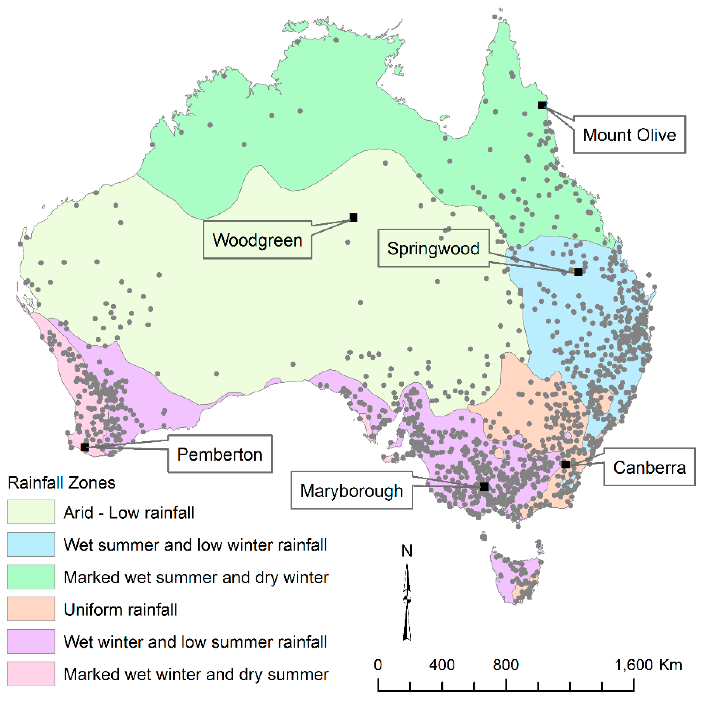
2.1. Data

The study analysed rainfall data from 1327 gauging stations across Australia having continuous long rainfall records. Daily rainfall data were obtained from the Bureau of Meteorology (BoM; http://www.bom.gov.au/). All data were checked for continuity and if any missing value was found, data for that particular year were excluded from the analysis. The final data set consisted of 92.8 years of data on average with minimum of 55 years and the maximum of 109 years. Rainfall across the study area varies significantly based on location and climate type. For the studied stations, the mean of monthly mean rainfall ranged from 11.39 mm to 321.33 mm. On an average, 6.6% of months in a year were found dry with maximum up to 55.1%. An in depth analyses on rainfall totals were conducted for six case study stations. The case study stations were selected to represent a variety of rainfall regimes in Australia (Figure 1). Woodgreen is from arid climate zone, while Canberra has a fairly uniform distribution of rainfall throughout the year. Though both Mount Olive and Springwood are from summer dominated rainfall regions, the winter for Mount Olive is drier, and the mean rainfall significantly higher than that for Springwood. Maryborough and Pemberton are from winter dominated rainfall regions, with Pemberton having a significantly high mean rainfall. To compare the distributions for the finer and the coarse time scale, the daily rainfall was accumulated to monthly and for four seasons (autumn: March, April, May; winter: June, July, August; spring: September, October, November; summer: December, January, February).
Variations in average, dispersion and extreme rainfall events have been observed between the case study stations. For example, mean daily rainfall range from 0.80 mm for Woodgreen to 4.41mm for Mount Olive. Spread in seasonal rainfall totals, as measured by co-efficient of variation, varied from 48.65% to 114.20% between the stations (Table 1). Extreme monthly rainfall totals as measured by 95th percentiles vary from 96.0 mm for dry station (Woodgreen) to 545.9 mm for wet tropical summer dominated station (Mount Olive).
All statistical analyses were conducted using the open access statistical software, R [29]. This software is freely available without any licence agreement and the software can be downloaded through the R-project web portal (http://www.R-project.org). The tweedie package [30] within the R environment was used to fit statistical models.

2.2. Methods

The study investigated a subfamily of exponential dispersion model (EDM) family of distributions to model daily, monthly and seasonal rainfall totals of Australia. The variable y (e.g., daily, monthly or seasonal rainfall totals) following the EDM family of distributions has the probability function:
f ( y ; θ , ϕ ) = a ( y , ϕ )   e x p [ 1 ϕ { y θ κ ( θ ) } ]
where θ is the canonical parameter and ϕ the dispersion parameter, a and k are suitable functions of θ and ϕ to link the variable y to an exponential probability function. The parameter θ can be positive or negative while ϕ is always positive [31].
Tweedie distributions are those EDMs for which variances are proportional to some power (p, also called index parameter) of the mean and have been used for modelling rainfall totals of Australia, Malaysia and India [7,32,33]. The Tweedie distribution with mean µ, dispersion parameter ϕ and index parameter p is dehnoted as T w p ( μ ,   ϕ ) ;   p ( 0 , 1 ) . Important properties of the Tweedie distributions are documented in scientific literature [34,35]. The normal (p = 0), Poisson (p = 1, ϕ = 1), gamma (p = 2) and inverse Gaussian (p = 3) distributions are special cases of Tweedie distributions. For (p ≥ 2), the distributions are suitable for modelling positive, right-skewed data. The distributions for which 1 < p < 2, are called the Poisson-Gamma (or P-G) distributions [36] and are capable of modelling positive rainfall data that include zero values (days with no rainfall). Dunn and Smyth [36] have shown theoretically that sometimes the maximum likelihood estimate of p is found on the boundary of the parameter space so that   p 1 . One interpretation is that the normal distribution (p = 0) may be optimal within the Tweedie family (as the Tweedie distribution is not defined for 0 < p < 1. No application of negative p values has been proposed in modelling rainfall. Except for four special cases, the Tweedie probability function cannot be written in closed form, and hence, maximum likelihood estimates of the parameters cannot be obtained directly. Therefore, the tweedie.profile function of R package tweedie initially considers a set of values for the index parameter, and computes the log-likelihood. The maximum likelihood value of the parameter is obtained from the plot of the log-likelihood against index parameter.
The models were fitted with the first half of the available data series and the rest were kept for validation purpose. Stochastic datasets were generated using the distributions and parameters obtained from the fitted models. The statistics, 5th, 25th, 95th, 99th percentiles and probability of no rainfall of observed (validated dataset) and generated rainfall amounts were compared.

3. Results

For the six case study stations, estimated p-indices, dispersion parameters (ϕ) and optimal probability distributions within the Tweedie family are presented in Table 2. Within the family, P-G distributions were found to be optimal for modelling daily rainfall totals for all case study stations. The monthly rainfall totals for Pemberton and seasonal rainfall totals for Springwood, Mount Olive, Maryborough and Pemberton, the p-indices were greater than but close to two, and hence, Gamma distributions were considered as near-optimal within the Tweedie family. It is notable that, even for strictly positive rainfall totals, P-G distribution may be optimal within the Tweedie family. In these situations, the studied data series may not include dry event; however, the model allows the possibility of getting future dry events.
Based on 1327 stations studied, within the Tweedie family, P-G distributions were found optimal for modelling the daily rainfall at any location. For monthly rainfall totals, P-G distributions were found optimal for 97.8% of stations and Gamma distributions were found near-optimal for the remaining gauges. For seasonal rainfall totals, the P-G, Gamma and Normal distributions were found optimal for 71.4%, 27.0% and 1.6% of stations respectively. For the cases where P-G distributions were optimal, the median of p-indices for daily, monthly and seasonal rainfall totals were 1.53, 1.58 and 1.71 respectively. Relatively smaller and consistent p-indices were noticed for models fitted to the daily rainfall data compared to those for monthly and seasonal timescales. The median dispersion parameters for the models fitted to the daily, monthly and seasonal rainfall were 10.95, 3.85 and 1.62 respectively (Figure 2). Relatively smaller ϕ-indices were found for cases where gamma distributions were optimal.

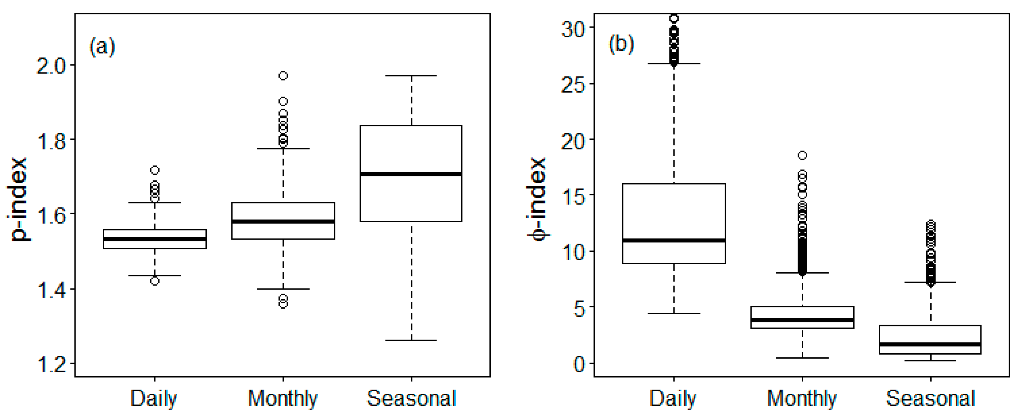
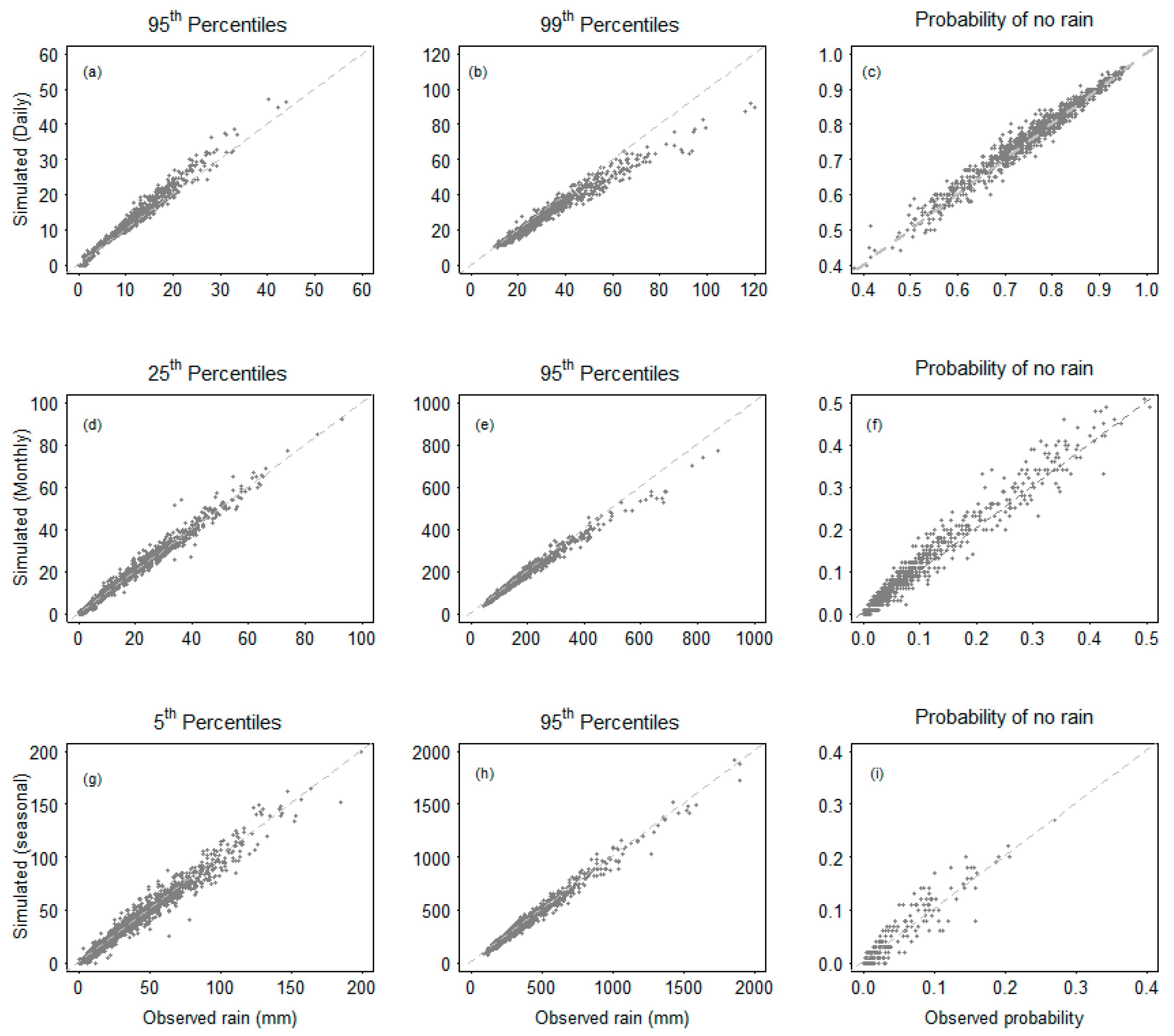
3.1. Comparing the Fit of the Model Using Tweedie Distributions

Once the optimal distribution within the Tweedie family and the parameters are obtained, the performance of the models in generating extreme events have been examined. For the purpose, statistics representing extreme rainfall event for validated and simulated data have been compared. Considering large proportion of dry days, the 95th and 99th percentiles of daily rainfall totals have been compared. Whereas, for monthly rainfall totals, 25th and 95th percentiles, and for seasonal rainfall totals 5th and 95th percentiles have been compared. The probabilities of no rainfall have been compared for all timescales. For validating, at each timescale and station, 1000 samples were generated using respective distributions and fitted parameters. The abovementioned statistics were estimated for each of the samples. Thus, for a specific timescale and station, 1000 values of each statistic were obtained. Medians of the statistics from all samples were then computed and compared with the statistics of validation data of respective timescale and station (Figure 3).
The models slightly overestimate 95th percentiles and underestimate 99th percentiles of daily and 95th percentiles of monthly rainfall totals. The models generate data reasonably well when considering the other percentiles considered in the analysis. While considering the probability of no rainfall, the models generate data reasonably well for all timescales. The extreme rainfall amounts, for example the 99th percentiles of daily and 95th percentiles monthly rainfall have a long tail and so usual distributions cannot capture well the extreme events. Extreme value distributions, such as, the Weibull, the generalised Pareto and the three-parameter log-normal, may be useful to fit such data. However, these distributions do not capture the lower parts of the data, that is, the major portion of the dataset. The mixture of models may perform better to capture both extremes of datasets; however, the approach requires extra parameters which may lead to a higher degree of parameter uncertainty in the modelling. The three parameter Tweedie models make a balance in the sense that, they capture well the probability of no rain and lower parts of the datasets and reasonably well the extremely high events.

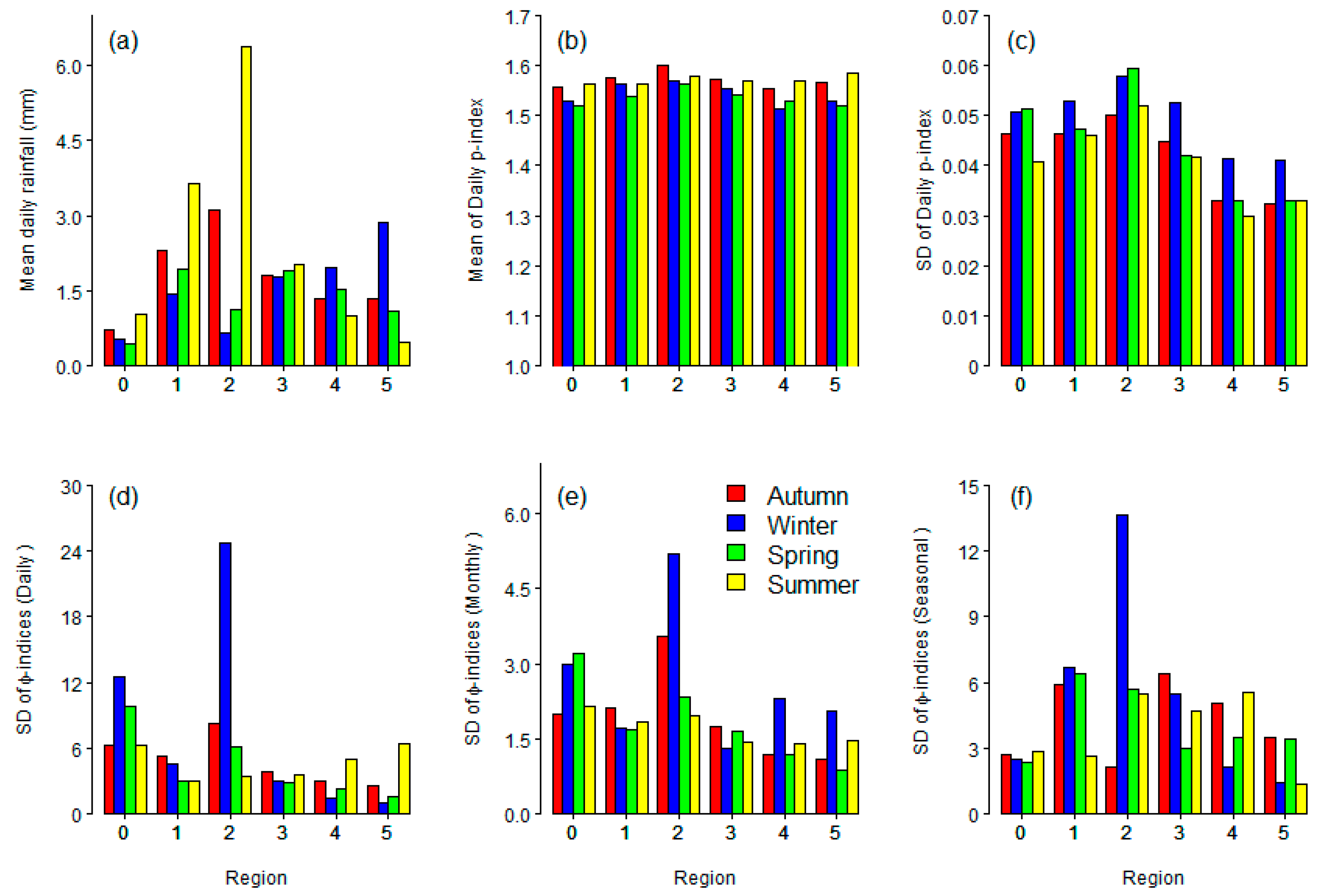
3.2. Spatial and Seasonal Variations of Parameters

The parameters of fitted models were compared for regions with diverse rainfall climate as defined by the BoM. From the arid zone (middle and parts of west coast of the country), 104 stations were considered. Next, 323 stations were studied from parts of mid-east coast that represent climate with wet summer and low winter rainfall. The north regions, with 76 studied stations, represent rainfall climate with wet summer and dry winter. From the regions with fairly uniform seasonal rainfall totals, 225 stations were studied. The largest sample of rainfall stations (504) were in regions with wet winter and low summer rainfall climate. Finally, 95 stations were considered from regions with wet winter and dry summer.
As shown in the top-left panel of Figure 4, seasonal variations in the mean rainfall amounts were evident across the studied regions. For the models fitted to daily rainfall, consistent p-indices have been observed across the regions and over the seasons (middle and right -top panels). Standard deviations of the dispersion parameters are presented in the bottom panels of Figure 4. Compared to daily or seasonal rainfall, relatively lower variation in the dispersion parameter were observed for monthly timescale. The largest and most inter-seasonal variations in the standard deviation of dispersion parameters was observed for the stations located in the dry and summer dominated northern regions. Highest dispersion parameters were observed for winter rainfall, especially in the arid and summer dominated regions. Significant seasonal variations in estimated parameters demands fitting separate models to individual seasons.

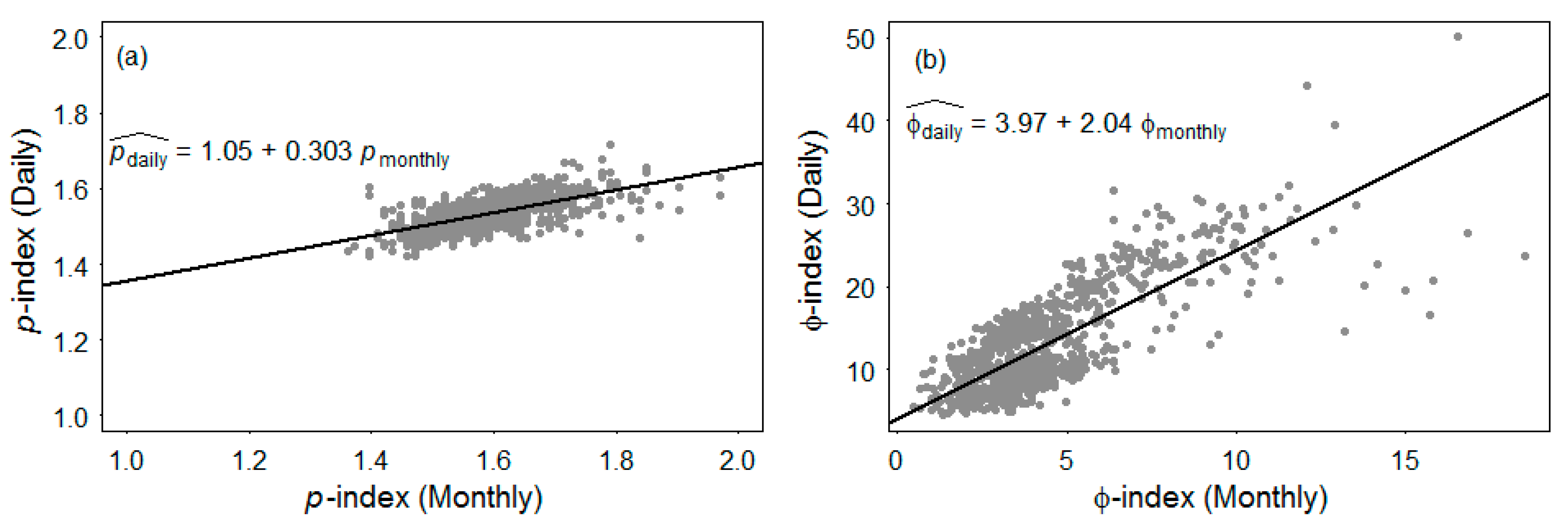
3.3. Estimating Parameters for Seasonal Models Using the Combined Model and Daily Timescales Form Monthly Timescale

This study aimed at exploring the possibility of generating rainfall data for individual seasons using estimated parameters based on annual total rainfall. For this purpose, the correlation coefficient (r) between the parameters from the overall datasets and those from individual seasons were estimated. Relatively weak relationship (r = 0.39) between ϕ-indices obtained from the fit of overall and winter daily models was observed. The reason may be the higher variations in the estimated dispersion parameters for the season. Strong relationships among the parameters (r = 0.70–0.91) for other seasons justify the possibility of predicting the parameters to individual seasons from those obtained from combined data. Table 3 represents results from the fitted linear models. The regression parameters are statistically significant for all cases, hence, the parameters for individual seasons can be estimated from the parameters of combined dataset.
Scatterplots in Figure 5 represent the relationships between parameters obtained from daily and monthly timescales. Strong correlation between daily and monthly p-indices have been observed (left panel). Regression equations have been fitted to predict parameters for daily data using the parameters for monthly parameters. Statistically significant positive slope parameters have been observed for both models. The results confirm that parameters for daily timescale can be predicted using the parameters obtained through models fitted to monthly data.
Simulated data obtained with the parameters of fitted models have similar characteristics (probability of no rainfall, extreme rainfall events) of observed data. However, the models slightly overestimate the 95th percentiles of daily rainfall and underestimate the 99th percentiles of daily and 95th percentiles of monthly rainfall totals. The results indicate that, the heavy right tail of the observed data with extreme events may not be covered well by the proposed model. Larger variations in rainfall amounts over the seasons and across the regions were obvious for the studied stations. However, the mean and standard deviations of p-indices were consistent in all cases. Standard deviations of ϕ-indices were more consistent for the monthly models than daily or seasonal model. Higher values in the dispersion parameter of daily data may be due to higher variation in the datasets, whereas, the variations in the seasonal models may be because of smaller sample size. Higher variations in the parameter were obtained for the stations from arid and summer dominated rainfall regions, and for winter seasons. Strong correlation, and significant slope parameters between the combined dispersion parameter data and those from individual seasons indicate the possibility of estimating the parameters for individual seasons from those estimated from combined data. The results also justify the possibility of estimating parameter for daily data using fitted parameters of monthly data.

4. Conclusions

Advanced statistical models have been fitted to data from 1327 gauging stations with reasonably long continuous rainfall records to test the applicability of different probability distribution functions. Within the Tweedie subfamily of EDM family, the P-G distributions were found optimal for majority of rainfall stations, whereas, normal distributions were rarely optimal. Fitted models have produced similar rainfall totals as observed. However, the models slightly overestimate the 95th percentiles of daily rainfall and underestimate the 99th percentiles of daily and 95th percentiles of monthly rainfall totals. Results indicate observed rainfall with extreme events may not be well captured by the fitted model. Findings of this study justify the possibility of estimating parameter for daily data using fitted parameters of monthly data. This may help to understand the probabilistic nature of rainfall totals across the different climatological regions of Australia, and potentially could help in other parts of the globe with similar climates. The exception is cold zone climates, where further testing of the approach would be necessary. More importantly, the relationship established between the parameter from monthly and daily models may help understanding the features and generating data to a daily timescale.

Author Contributions

This study was conceptualized by M.M.H. and B.F.W.C.; methodology was formulated and executed by M.M.H. and B.F.W.C.; resources including data were collected and processed by M.M.H. and F.K.; The manuscript was written jointly by M.M.H., B.F.W.C. and F.K.

Funding

This work was funded by the National Centre for Groundwater Research and Training, a collaborative initiative of the Australian Research Council and the National Water Commission.

Conflicts of Interest

The authors declare no conflict of interest.

References

  1. Beskow, S.; Caldeira, T.L.; de Mello, C.R.; Faria, L.C.; Guedes, H.A.S. Multiparameter probability distributions for heavy rainfall modeling in extreme Southern Brazil. J. Hydrol.-Reg. Stud. 2015, 4, 123–133. [Google Scholar] [CrossRef]
  2. Hailegeorgis, T.T.; Thorolfsson, S.T.; Alfredsen, K. Regional frequency analysis of extreme precipitation with consideration of uncertainties to update idf curves for the city of Trondheim. J. Hydrol. 2013, 498, 305–318. [Google Scholar] [CrossRef]
  3. Baigorria, G.A.; Jones, J.W. Gist: A stochastic model for generating spatially and temporally correlated daily rainfall data. J. Clim. 2010, 23, 5990–6008. [Google Scholar] [CrossRef]
  4. Hasan, M.M.; Dunn, P.K. Entropy, consistency in rainfall distribution and potential water resource availability in Australia. Hydrol. Processes 2011, 25, 2613–2622. [Google Scholar] [CrossRef]
  5. Nowak, G.; Welsh, A.; O’Neill, T.; Feng, L. Spatio-temporal modelling of rainfall in the murray-darling basin. J. Hydrol. 2018, 557, 522–538. [Google Scholar] [CrossRef]
  6. Shukla, S.; McNally, A.; Husak, G.; Funk, C. A seasonal agricultural drought forecast system for food-insecure regions of East Africa. Hydrol. Earth Syst. Sci. 2014, 18, 3907–3921. [Google Scholar] [CrossRef] [Green Version]
  7. Hasan, M.M.; Croke, B. Filling gaps in daily rainfall data: A statistical approach. In Proceedings of the 20th International Congress on Modelling and Simulation, Adelaide, Australia, 1–6 December 2013. [Google Scholar]
  8. Rosenberg, K.; Boland, J.; Howlett, P.G. Simulation of monthly rainfall totals. ANZIAM J. 2008, 46, 85–104. [Google Scholar] [CrossRef]
  9. Lee, J.; Kim, S.; Jun, H. A study of the influence of the spatial distribution of rain gauge networks on areal average rainfall calculation. Water 2018, 10, 1635. [Google Scholar] [CrossRef]
  10. Camberlin, P.; Gitau, W.; Oettli, P.; Ogallo, L.; Bois, B. Spatial interpolation of daily rainfall stochastic generation parameters over East Africa. Clim. Res. 2014, 59, 39–60. [Google Scholar] [CrossRef]
  11. Chowdhury, A.; Lockart, N.; Willgoose, G.; Kuczera, G.; Kiem, A.S.; Manage, N.P. Modelling daily rainfall along the east coast of australia using a compound distribution markov chain model. In Proceedings of the 36th Hydrology and Water Resources Symposium: The Art and Science of Water, Hobart, Australia, 7–10 December 2015; Engineers Australia: Barton, Australia, 2015; p. 625. [Google Scholar]
  12. Rajah, K.; O’Leary, T.; Turner, A.; Petrakis, G.; Leonard, M.; Westra, S. Changes to the temporal distribution of daily precipitation. Geophys. Res. Lett. 2014, 41, 8887–8894. [Google Scholar] [CrossRef] [Green Version]
  13. Liang, L.; Zhao, L.; Gong, Y.; Tian, F.; Wang, Z. Probability distribution of summer daily precipitation in the huaihe basin of China based on gamma distribution. Acta Meteorol. Sin. 2012, 26, 72–84. [Google Scholar] [CrossRef]
  14. Piantadosi, J.; Boland, J.; Howlett, P. Generating synthetic rainfall on various timescales—Daily, monthly and yearly. Environ. Model. Assess. 2009, 14, 431–438. [Google Scholar] [CrossRef]
  15. Papalexiou, S.M.; Koutsoyiannis, D. A global survey on the seasonal variation of the marginal distribution of daily precipitation. Adv. Water Resour. 2016, 94, 131–145. [Google Scholar] [CrossRef]
  16. Mandal, S.; Choudhury, B. Estimation and prediction of maximum daily rainfall at sagar island using best fit probability models. Theor. Appl. Climatol. 2015, 121, 87–97. [Google Scholar] [CrossRef]
  17. Li, Z.; Brissette, F.; Chen, J. Assessing the applicability of six precipitation probability distribution models on the loess plateau of China. Int. J. Climatol. 2014, 34, 462–471. [Google Scholar] [CrossRef]
  18. Suhaila, J.; Jemain, A. Fitting the statistical distribution for daily rainfall in peninsular malaysia based on aic criterion. J. Appl. Sci. Res. 2008, 4, 1846–1857. [Google Scholar]
  19. Borwein, J.; Howlett, P.; Piantadosi, J. Modelling and simulation of seasonal rainfall using the principle of maximum entropy. Entropy 2014, 16, 747–769. [Google Scholar] [CrossRef]
  20. Ghosh, S.; Roy, M.K.; Biswas, S.C. Determination of the best fit probability distribution for monthly rainfall data in Bangladesh. Am. J. Math. Stat. 2016, 6, 170–174. [Google Scholar]
  21. Kossieris, P.; Makropoulos, C.; Onof, C.; Koutsoyiannis, D. A rainfall disaggregation scheme for sub-hourly time scales: Coupling a bartlett-lewis based model with adjusting procedures. J. Hydrol. 2018, 556, 980–992. [Google Scholar] [CrossRef]
  22. Pal, S.; Mazumdar, D. Stochastic modelling of monthly rainfall volume during monsoon season over gangetic west Bengal, India. Nat. Environ. Pollut. Technol. 2015, 14, 951–956. [Google Scholar]
  23. Yue, S.; Hashino, M. Long term trends of annual and monthly precipitation in Japan. JAWRA J. Am. Water Resour. Assoc. 2003, 39, 587–596. [Google Scholar] [CrossRef]
  24. Abtew, W.; Melesse, A.M.; Dessalegne, T. El niño southern oscillation link to the blue nile river basin hydrology. Hydrol. Processes 2009, 23, 3653–3660. [Google Scholar] [CrossRef]
  25. Husak, G.J.; Michaelsen, J.; Funk, C. Use of the gamma distribution to represent monthly rainfall in Africa for drought monitoring applications. Int. J. Climatol. 2007, 27, 935–944. [Google Scholar] [CrossRef] [Green Version]
  26. Rader, M.; Kirshen, P.; Roncoli, C.; Hoogenboom, G.; Ouattara, F. Agricultural risk decision support system for resource-poor farmers in Burkina Faso, West Africa. J. Water Resour. Plan. Manag. 2009, 135, 323–333. [Google Scholar] [CrossRef]
  27. Hasan, M.M.; Dunn, P.K. Two tweedie distributions that are near-optimal for modelling monthly rainfall in Australia. Int. J. Climatol. 2011, 31, 1389–1397. [Google Scholar] [CrossRef]
  28. Hasan, M.M.; Dunn, P.K. Seasonal rainfall totals of Australian stations can be modelled with distributions from the tweedie family. Int. J. Climatol. 2015, 35, 3093–3101. [Google Scholar] [CrossRef]
  29. Ihaka, R.; Gentleman, R. R: A language for data analysis and graphics. J. Comput. Graph. Stat. 1996, 5, 299–314. [Google Scholar]
  30. Dunn, P. Tweedie: Tweedie Exponential Family Models; R Package Version 2.2.1; R Core Team: Vienna, Austria, 2014. [Google Scholar]
  31. McCullagh, P.; Nelder, J. Generalized Linear Models; Chapman & Hall: New York, NY, USA, 1989. [Google Scholar]
  32. Saha, K.; Hasan, M.; Quazi, A. Forecasting tropical cyclone-induced rainfall in coastal Australia: Implications for effective flood management. Australas. J. Environ. Manag. 2015, 22, 446–457. [Google Scholar] [CrossRef]
  33. Yunus, R.M.; Hasan, M.M.; Razak, N.A.; Zubairi, Y.Z.; Dunn, P.K. Modelling daily rainfall with climatological predictors: Poisson-gamma generalized linear modelling approach. Int. J. Climatol. 2017, 37, 1391–1399. [Google Scholar] [CrossRef]
  34. Dunn, P.K. Occurrence and quantity of precipitation can be modelled simultaneously. Int. J. Climatol. 2004, 24, 1231–1239. [Google Scholar] [CrossRef] [Green Version]
  35. Jiang, J. Linear and Generalized Linear Mixed Models and Their Applications; Springer Science & Business Media: Berlin, Germany, 2007. [Google Scholar]
  36. Dunn, P.K.; Smyth, G.K. Series evaluation of tweedie exponential dispersion model densities. Stat. Comput. 2005, 15, 267–280. [Google Scholar] [CrossRef]
Figure 1. Map of Australia showing rainfall zones, locations of the studied stations (grey dots). The case study stations are named and represented by black squares.
Climate 07 00004 g001
Figure 2. Boxplots representing Q1 (first quartile, bottom edge of the box), median (thick horizontal line in the middle), Q3 (third quartile, top edge of the box) and outliers (circles) for: (a) index parameter (p) and (b) dispersion parameter (ϕ) for the 1327 stations at various timescales.
Climate 07 00004 g002
Figure 3. Scatterplots of simulated and observed (validated) rainfall for 95th, 99th percentiles and probability of no rain for daily data (plots a, b and c respectively), 25th, 95th percentiles and probability of no rain for monthly data (plots d, e and f respectively) and 5th, 99th percentiles and probability of no rain for seasonal data (plots g, h and i respectively).
Climate 07 00004 g003
Figure 4. Plots representing mean daily rainfall, mean and SD of p-index for daily model (plots a, b and c respectively) and SD of ϕ-index for daily, monthly and seasonal data (plots d, e and f respectively) for all studied timescales over the seasons and across regions of Australia.
Climate 07 00004 g004
Figure 5. Scatterplots representing the relationships between monthly and daily p-indices (a) and ϕ-index (b) for the 1327 gauging stations.
Climate 07 00004 g005
Table 1. Statistics of rainfall totals at various timescales for six case study stations.
StationsDailyMonthlySeasonal
Mean (mm)CV *% Zero95th PercentileCV *% Zero95th PercentileCV *% Zero95th Percentile
Woodgreen0.80619.6493.053.0174.2837.8696.0114.209.26208.85
Mount Olive4.41345.1570.8126.6137.778.18545.999.830.911176.73
Springwood1.92430.1287.0011.9118.5911.76200.987.391.41461.98
Canberra1.69331.5770.0310.276.890.35125.748.650275.60
Maryborough1.42312.5368.938.173.470.9297.749.300248.69
Pemberton3.18212.1451.8117.884.150240.767.900631.56
* coefficient of variation.
Table 2. Index parameter (p) values, optimal distribution function within the Tweedie family and dispersion parameters (ϕ) values of daily, monthly and seasonal rainfall data for the six case study stations.
StationsDailyMonthlySeasonal
p ValueDistributionϕpDistributionϕpDistributionϕ
Woodgreen1.46P-G26.871.49P-G10.861.56P-G6.70
Springwood1.51P-G19.271.64P-G5.152.29Gamma0.17
Mount Olive1.62P-G13.931.74P-G5.832.20Gamma0.45
Canberra Airport Comparison1.63P-G8.721.67P-G2.041.87P-G0.45
Maryborough1.54P-G7.991.58P-G2.762.10Gamma0.17
Pemberton1.58P-G6.622.07Gamma0.732.13Gamma0.28
Table 3. Correlation and regression coefficients of fitted models of seasonal parameters on the parameters for combined data. Separate results have been presented for p- and ϕ-indices.
p-Indexϕ-Index
Correlation CoefficientRegression CoefficientsCorrelation CoefficientRegression Coefficients
ConstantSlope (SD *)ConstantSlope (SD *)
Autumn0.760.380.75 (0.01) a0.91−0.610.99 (0.01) a
Winter0.700.600.63 (0.12) a0.3910.800.40 (0.03) a
Spring0.810.350.79 (0.02) a0.940.871.04 (0.01) a
Summer0.770.120.92 (0.02) a0.72−5.671.39 (0.04) a
* SD = Standard Deviation; a: Significant at less than 0.01 level.

