Article

Decadal Ocean Heat Redistribution Since the Late 1990s and Its Association with Key Climate Modes

1
International Center for Climate and Environment Sciences, Institute of Atmospheric Physics, Chinese Academy of Sciences, Beijing 100029, China
2
College of Meteorology and Oceanography, National University of Defense Technology, Nanjing 210001, China
3
School of Engineering, University of St. Thomas, St. Paul, MN 55105, USA
4
State Key Laboratory of Numerical Modeling for Atmospheric Sciences and Geophysical Fluid Dynamics, Institute of Atmospheric Physics, Chinese Academy of Sciences, Beijing 100029, China
5
University of Chinese Academy of Sciences, Beijing 100049, China
*
Author to whom correspondence should be addressed.
Climate 2018, 6(4), 91; https://doi.org/10.3390/cli6040091
Submission received: 15 October 2018 / Revised: 8 November 2018 / Accepted: 15 November 2018 / Published: 19 November 2018
(This article belongs to the Special Issue Postmortem of the Global Warming Hiatus)

Abstract

:
Ocean heat content (OHC) is the major component of the earth’s energy imbalance. Its decadal scale variability has been heavily debated in the research interest of the so-called “surface warming slowdown” (SWS) that occurred during the 1998–2013 period. Here, we first clarify that OHC has accelerated since the late 1990s. This finding refutes the concept of a slowdown of the human-induced global warming. This study also addresses the question of how heat is redistributed within the global ocean and provides some explanation of the underlying physical phenomena. Previous efforts to answer this question end with contradictory conclusions; we show that the systematic errors in some OHC datasets are partly responsible for these contradictions. Using an improved OHC product, the three-dimensional OHC changes during the SWS period are depicted, related to a reference period of 1982–1997. Several “hot spots” and “cold spots” are identified, showing a significant decadal-scale redistribution of ocean heat, which is distinct from the long-term ocean-warming pattern. To provide clues for the potential drivers of the OHC changes during the SWS period, we examine the OHC changes related to the key climate modes by regressing the Pacific Decadal Oscillation (PDO), El Niño-Southern Oscillation (ENSO), and Atlantic Multi-decadal Oscillation (AMO) indices onto the de-trended gridded OHC anomalies. We find that no single mode can fully explain the OHC change patterns during the SWS period, suggesting that there is not a single “pacemaker” for the recent SWS. Our observation-based analyses provide a basis for further understanding the mechanisms of the decadal ocean heat uptake and evaluating the climate models.

1. Introduction

Recent changes in global mean surface temperature (GMST) or sea surface temperature (SST) change have been heavily debated in the past ten years, because of an occurrence of a period (1998–2013) with a slower increase in both the GMST and SST compared to the long-term trend (i.e., since 1951) or than the previous decade (1983–1997) [1] (Figure 1). This phenomenon has been termed as a so-called “global warming hiatus” or “surface temperature hiatus” in many literature references [2,3,4,5,6,7,8]. The use of these terms immediately raises a question. Does it indicate the slowdown of the human-induced global warming driven by the accumulation of greenhouse gases (GHG) in the climate system since industrial revolution, which is well established in the climate community [9,10]?
It is important to articulate a clear meaning to the “hiatus” description. In the scientific community, it generally describes a change in the range of surface warming that is outside the bounds of natural fluctuations superimposed upon a long-term trend. The requirement of statistical significance allows research tools to be used to determine whether or not some slowdown has occurred. Over the past few years, many studies have looked at this very issue. For instance, Karl et al. [11], discovered artifacts in temperature measurements that, when accounted for, showed a significant increase in warming rate. Among the artifacts were differences in ship-based and buoy-based sensors and accounting for these differences. In addition, historical changes in the SST, in particular changes to measurement techniques circa 1940s were quantified and addressed. Finally, Karl et al. [11] used an updated land-temperature dataset. The end result of these corrections was that over the preceding 17 years, GMST had increased without a halt, and in fact, had increased at a steady rate.
A series of other studies applied multiple and independent statistical tests to the GMST record and demonstrated, conclusively, that there is no statistically significant decrease in the rate of surface warming and that the rate of warming within the past two decades is not unusual in a continuously warming world [12,13,14,15]. The importance of differing definitions of a “hiatus” was discussed in Medhaug et al. [16] where contradictory conclusions can arise in the literature based on the definition. Consequently, elucidating the various different definitions of “pause” or “hiatus” is important.
Among the common definitions of pause/hiatus are: (1) a statistically significant change in the rate of global warming, as measured by changes to the heat balance of the planet; (2) a statistically significant change in the surface temperature record; (3) a non-statistically significant change in the rate of GMST change; and (4) Divergence between GMST predictions (from climate modes) and actual GMST measurements. Unfortunately, these definitions are often conflated and their separate identities must be maintained.
So, has there been a pause in global warming? The answer would be mistakenly “yes” only if one defines the “global warming” only by GMST changes (definition 3 above). Fundamentally, the global warming is caused by the Earth’s energy imbalance (EEI). During equilibrium climate states, the amount of incoming solar radiation is balanced by the outgoing radiation at the top of the atmosphere (TOA). However, increases in GHGs in the air trap more energy within the climate system, thus creating an imbalance of the Earth’s energy [17,18]. More heat available in the climate system is manifested in many ways including increasing the GMST/SST [19], increasing the ocean/land interior temperatures [20], raising the sea level [21], melting the ice sheets and permafrost [22], altering the hydrological cycle [23], changing the atmospheric and oceanic circulation [24], supporting stronger tropical cycles with heavier rainfall [25], among other “symptoms” of the global warming [9].
Due to its large heat capacity and huge volume, the ocean has a greater capability to store heat than the other components of the earth system (i.e., land, atmosphere). Actually, more than 90% of the EEI has been stored in the ocean [26]. This heat imbalance is manifested by the increase of ocean heat content (OHC). Therefore, from the energy point of view, the most fundamental metric for global warming is EEI and OHC [17,18,27,28]. Also OHC is a robust metric for global warming since it is much less impacted by the natural fluctuations of the climate system than is GMST on inter-annual scales [27].
Many studies have already shown that there is no slowdown in OHC records based on observational datasets [29,30], reanalysis products [31], and model simulations [32,33]. Instead, as presented in Figure 1, the rate of OHC increase is larger during the 1998–2013 period (0.98 ± 0.16 × 10²² J/yr, ~0.61 W m−2 averaged over the Earth’s surface) than the 1983–1997 period (0.70 ± 0.17 × 10²² J/yr, ~0.43 W m−2) and 1955–1997 period (0.30 ± 0.07 × 10²² J/yr, ~0.19 W m−2), consistent with the increase of GHG concentration in the atmosphere [10] (The 95% confidence interval for the linear trend is provided according to Foster and Rahmstorf [34]). Therefore, “global warming hiatus” to indicate a decrease in warming is misleading and has been misinterpreted; there is no slowdown in the global warming nor any decrease in the energy imbalance of the planet. It would be better to name the slowdown in the rate of GMST/SST during the 1983–1997 period as “surface warming slowdown” (SWS hereafter), which will be used in this study. And it is imperative to establish multiple climate indicators besides of GMST/SST as collected in last IPCC report [9].
With continuous warming of our climate, why was there a non-statistically significant slowing of the GMST/SST increase during the 1998–2013 period? The leading hypothesis is that this SWS was regulated by the natural variability generated near the air-sea interface, such as the Interdecadal Pacific Oscillation (IPO) or Pacific Decadal Oscillation (PDO) [35,36] in the Pacific Ocean and the Atlantic Multi-decadal Oscillation (AMO) [37] in the Atlantic Ocean. Some of the previous model-based studies reported that the tropical Pacific was the main “pacemaker” as the stronger trade winds in the central and eastern Pacific increased the cold water upwelling in the tropical eastern Pacific, which cools the local sea surface, and increases the warm water penetration into the ocean subsurface as the subtropical cell is strengthened [2,4,38]. The GMST/SST cooling induced by the tropical Pacific cooling offsets the warming effects in the other oceans, leading to weak warming rates [8]. However, other studies reported the importance of Atlantic and Southern Oceans [39], arguing that the sea surface slowdown is caused by heat transported to deeper layers driven by the change of the Atlantic Meridional Overturning Circulation. A detailed overview of the potential drivers of the SWS can be found in Liu et al. [40].
Many of these hypotheses relate surface changes (GMST/SST) to the ocean subsurface changes (OHC), as increased ocean heating driven by GHG must be sequestered in the ocean interior if it does not appear in the near surface layers (represented by GMST/SST). And then an outstanding question arises: where is the heat? What is the relationship between GMST/SST and OHC on decadal scales? This question is yet to be fully answered and a vigorous scientific debate has emerged. Palmer and McNeall [41] suggested that global OHC changes on a decadal scale is out of phase with GMST in the simulations of the fifth phase of the Coupled Model Inter-comparison Project (CMIP5). And many other studies tried to identify local OHC “hot spots” and hypothesized their role in global GMST/SST changes [32,39,42,43]. However, contradictory conclusions were drawn by these studies, highlighting different ocean basins for SWS. The contradictions in previous OHC-related studies is tied to two issues:
(1)
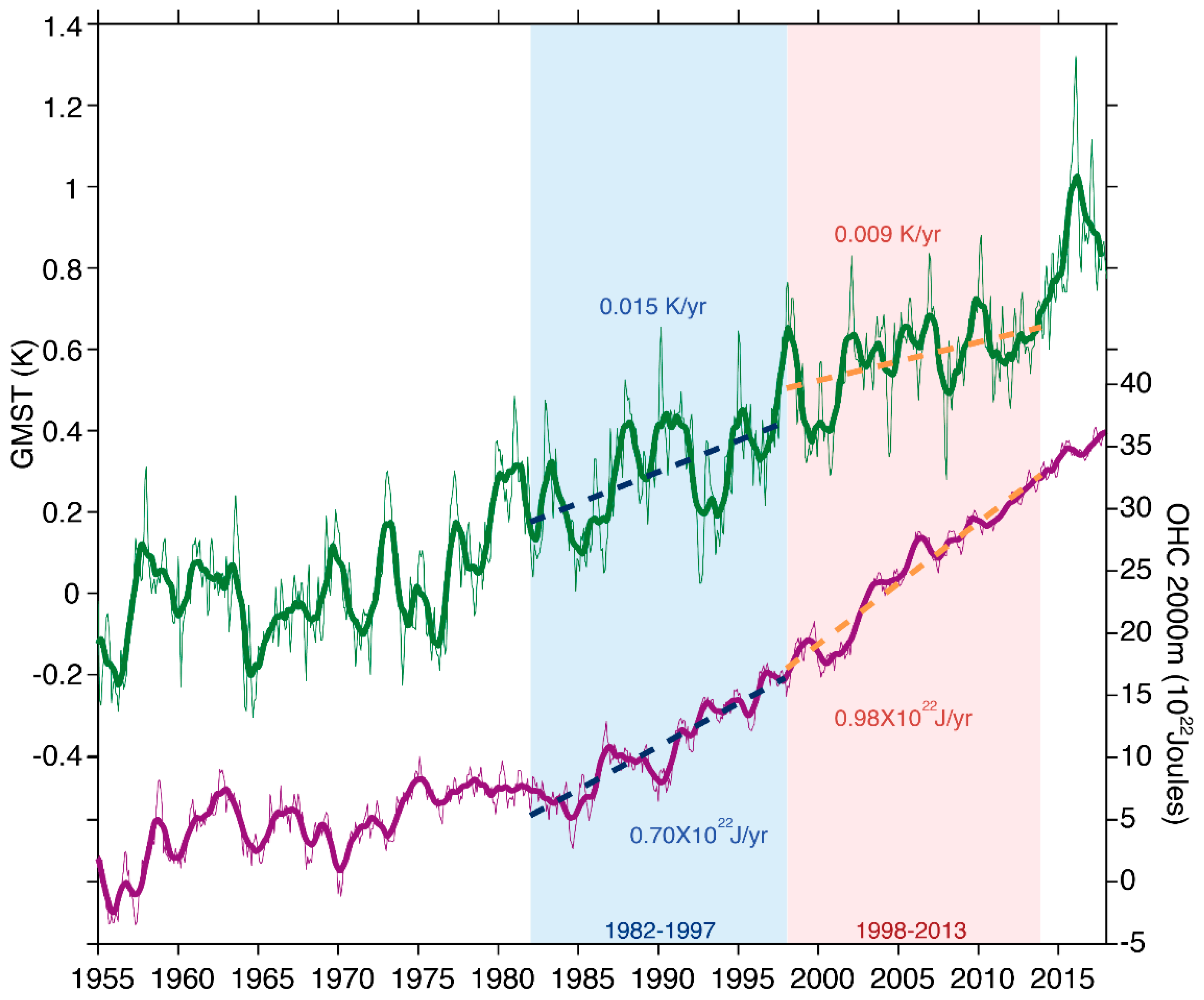
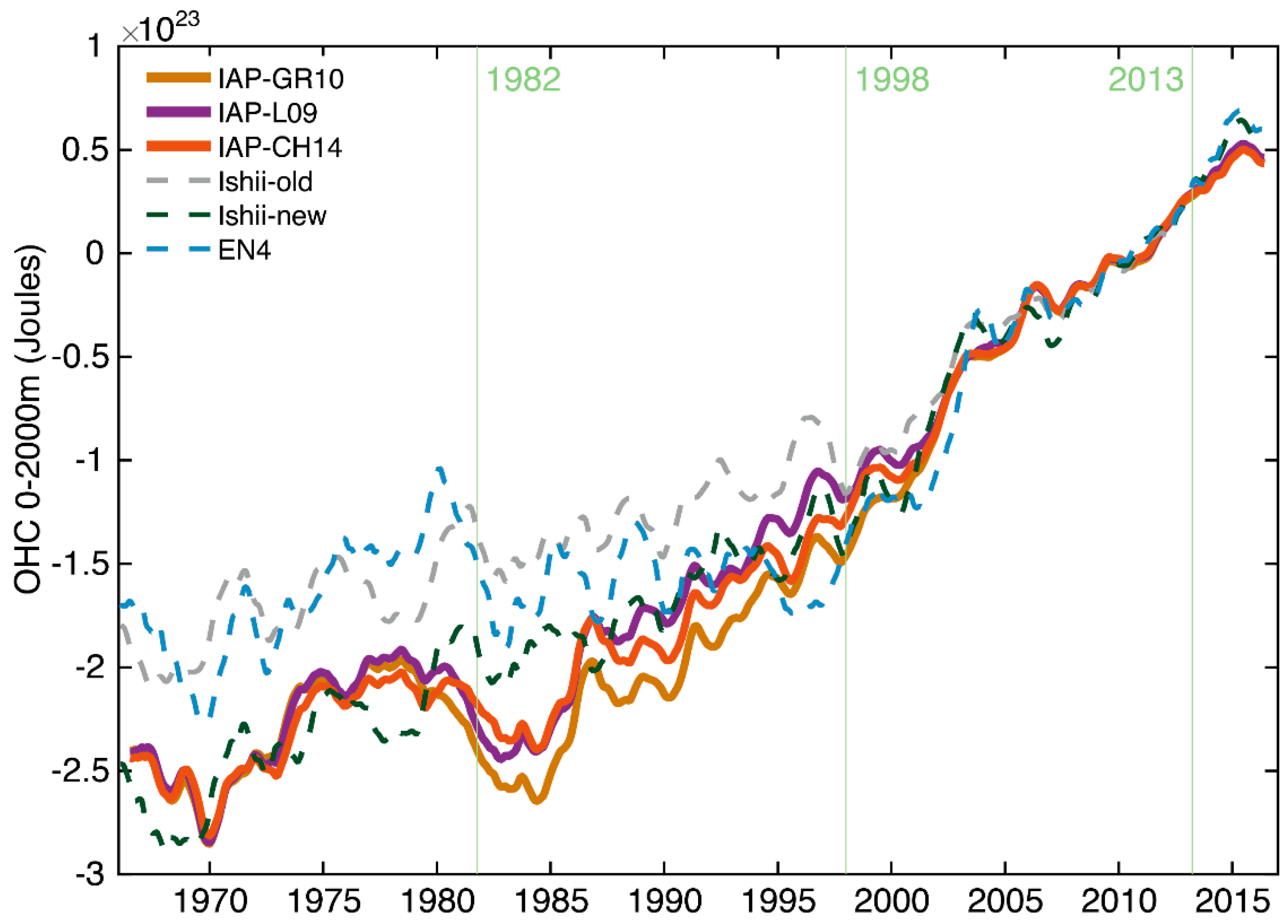
Uncertainties in OHC products, which are not fully accounted for in previous studies related to SWS. They were substantial differences among OHC datasets [26,44,45], which is one reason for the debate. Recently, progress has been made to understand the error in OHC estimates and improve the OHC record [29,46,47,48]. This progress will be discussed in Section 3 and will allow for a better identification of the OHC change during the SWS period.
(2)
On a decadal scale, natural variability in OHC records are mixed with forced changes by GHGs (manifested by a long-term warming trend in OHC), aerosols, ozone, volcanoes (manifested by a several-years decrease in OHC records) etc. [32,49,50,51,52,53]. Therefore, one has to separate the natural variability related to SWS from other changes such as a long-term anthropogenic warming signals. One method is to use climate models [32], but the short-coming of this approach is the model error at the ocean subsurface [54,55], resulting in some inconsistency among model-based studies [43,51,56]. This study used a simple method accounting for the forced changes (will be introduced in Section 2) the results will be shown in Section 3.
This study is organized as follows: data and methods will be introduced in Section 2. In the results section (Section 3), we will first revisit the improvements to OHC estimates and show the impact of OHC errors in investigating the surface warming hiatus (Section 3.1). Then we will quantify OHC changes based on improved ocean observations during the SWS period (1998–2013) and compare them with the 1982–1997 reference period. This decadal scale OHC change will also be compared with the long-term ocean warming (i.e., OHC change for 1955–2017). These comparisons will highlight the distinct pattern of the decadal ocean heat redistribution from the long-term trend (Section 3.2). In Section 3.3, potential links between the key modes of climate variability and OHC on decadal scales are investigated. Implications for the drivers of the ocean heat redistribution during the SWS period will be given. The conclusion and discussion are presented in the final Section 4.

2. Data and Method

An observational ocean temperature product from the Institute of Atmospheric Physics (IAP) [29,57] is used in this study. The IAP product has advantages in both instrumental bias correction (necessary to ensure high-quality observations) and mapping method (to provide a homogenous product with complete global ocean coverage). The instrumental bias refers to systematic errors in Expendable Bathythermograph (XBT) data [58]. It was clear that the major uncertainty in OHC record comes from two sources: bias corrections for XBT data and different choices made in the mapping method [48,59]. The impacts of these two advances on the SWS discussion will be discussed in Section 3.1. Other errors are either less understood (i.e., quality control for the data) or dependence on the performance of the mapping method (i.e., choice of climatology to calculate the anomaly field).
The IAP product uses a new XBT correction scheme which has been recommended by the XBT scientific community [46]. A mapping method uses the data only near the analyzed grid within an assumed area to perform the reconstruction at individual grid cells, with the size of the area defined by the influencing radius. The covariance defines the correlation between the analyzed grid with the adjacent locations, which are used in the reconstruction. The IAP mapping method uses the Ensemble Optimal Interpolation (EnOI) framework with first-guess and covariance from a number of CMIP5 simulations. Models provide more reliable covariance than the traditional parameterization, which always assumes a Gaussian distribution (e.g., in Levitus et al. [60] and Ishii et al. [61]). Use of models allows the choice of a larger “influencing radius” than previous methods, and ensures a near-global fractional coverage (defined as the fraction of total ocean area obtained by the mapping method).
For comparison, we also use two other gridded ocean temperature products constructed based on in-situ ocean observations and different mapping methods and XBT correction schemes. The first is Ishii data with two different versions: an old version first published in 2003 [61] (Ishii-old) and an improved version released in 2017 [47] (Ishii-new). Ishii-old data was used in many studies related to the “hiatus” [32,39,62] and has been discussed in follow-on communications [63,64]. Therefore, it is worthwhile to examine its quality in the present analysis. EN4 data from Met Office was also used in [62,65]. We will provide some analyses on these datasets in our study, but a more comprehensive comparison among these datasets can be found in Wang et al. [45] and a careful evaluation on IAP-mapping can be found in Cheng et al. [29].
Differences between the linear trends of the SWS period (1998–2013) and the reference period (1982–1997) are used to examine the ocean heat content redistribution related to SWS (this method is named “Trend-Diff method”). As discussed before, there is a substantial global warming (GHGs forced) signal in the OHC records which should be removed or reduced in order to show the natural variability. Using the trend differences reduces the impact of long-term anthropogenic warming, assuming the long-term warming is constant in time (especially during the 1982–2013 period). However, with more GHGs accumulating in the atmosphere over time, there should be an acceleration of long-term warming (nonlinear and non-constant), as shown in climate models [33]. Another way to consider the long term trend is to use the global mean time series as a primary indicator of the non-constant component, and remove it from each grid point prior to carrying out an analysis, as proposed in Trenberth and Shea [66] (this method is named “Glb-Trend-Remove method”). Both methods are tested in this study and show similar geographical patterns. Consequently, the result based on the first method is always shown.
The results could be sensitive to the choice of time-window, so we also tested the results by using several other choices (i.e., 1998–2012, 1999–2013, 2000–2013), showing that they do not impact the OHC pattern. All these methods and time-window choices impact the quantification of the OHC changes in different ocean basins, but the key conclusion remains unchanged.

3. Results

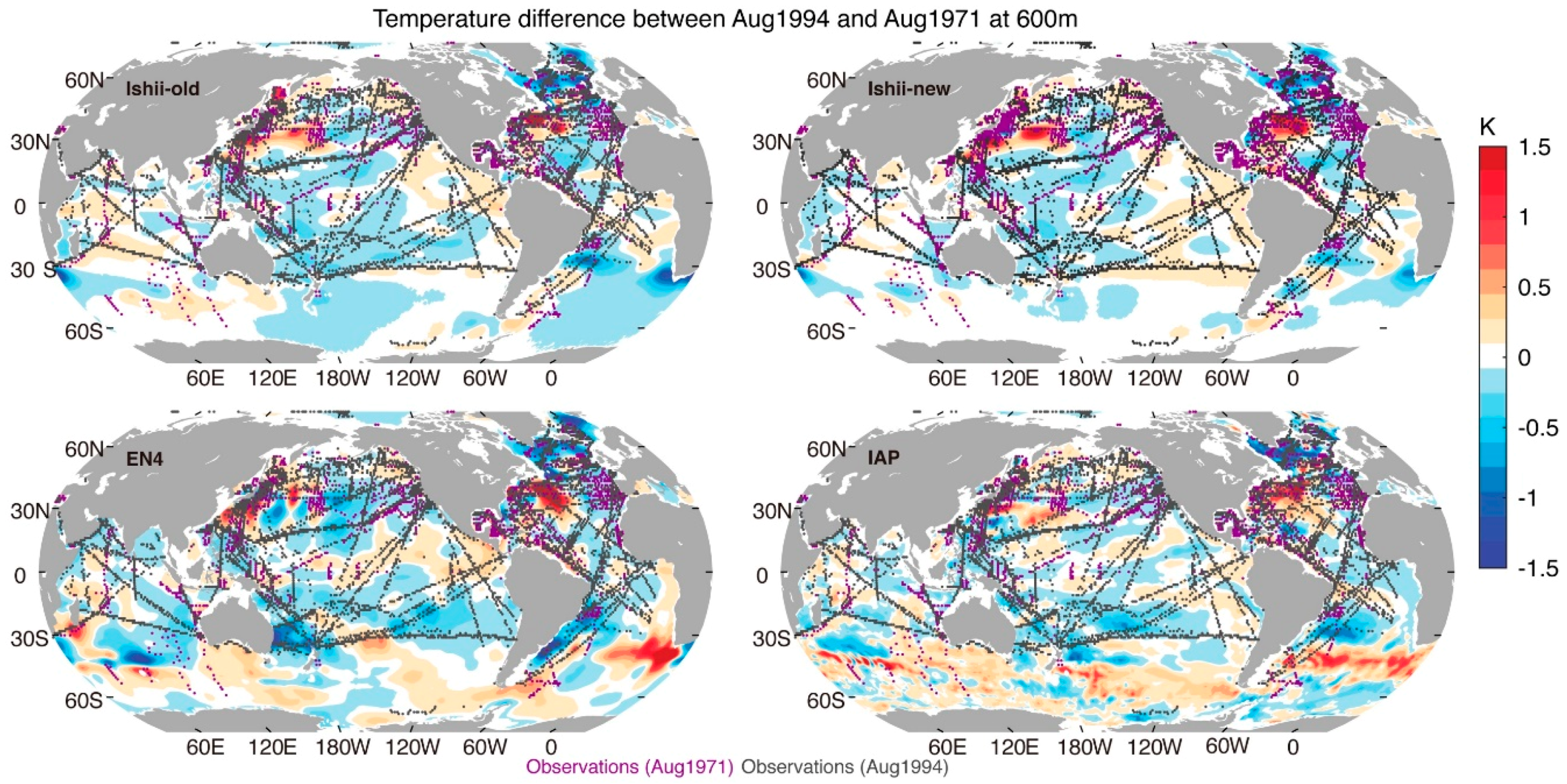
3.1. Improving the OHC Record

For XBT bias corrections, there have been more than ten correction schemes proposed since 2008 [46] and techniques to utilize metadata to identify probe types [67]. Some of them (for example, Ishii and Kimoto [68] used in Ishii-old and Ishii-new products) are not complete because only depth error is taken into account. In addition, there is also a temperature error [46]. The incompleteness of the correction schemes impact the long-term trend in OHC record [69]. Also, XBT bias has significant latitude dependency, a larger warm bias appears in the low latitudes with smaller errors in the higher latitudes. As a consequence, appropriately accounting for the XBT error is important for the examination of the regional OHC changes. Since 2014, the community has recommended the method proposed in Cheng et al. 2014 (CH14) [70] as the most complete correction for XBT data for calculating OHC, as it accounts for all of the known factors that influence XBT error and latitude-dependency of the error can be substantially reduced. Cheng et al. [69] identified three superior schemes for XBT bias correction that all reduce global mean bias. Using these three schemes results in consistent OHC changes since 1966 (Figure 2). Consequently, the uncertainty in OHC due to XBT error is reduced as a more complete understanding of the error sources and corrections are proposed and identified.
Many mapping methods used smaller “influencing radii” less than 10°, which results in smaller fractional coverage and a “conservative error” occurs in regions with major data gaps (mainly in the Southern Hemisphere) [73,74,75]. This error occurs because these methods infill climatological value (with zero anomaly) in the analyzed grid when there are no or insufficient adjacent observations located within a distance smaller than the specified “influencing radii”. An example is provided in Figure 3 which shows the temperature difference at the depth of 600-m between August 1971 and August 1998 with observation distribution indicated by dots in the plots. As expected, there are much less data in the Southern Hemisphere (70~30° S) in both 1971 and 1998. There appears to be near-zero temperature changes over the 27 years in these regions for Ishii-old, Ishii-new, and EN4 data, directly contradicting the significant Southern Ocean warming found in the literature using both observations and models [50,76,77,78]. Ishii-old, Ishii-new and EN4 also show very weak spatial variability in the data-sparse regions which are also not physically tenable because the Southern Ocean is one of the most active areas over the global ocean with rich eddy variability [79]. Calculating the difference between any two years before the Argo period yields similar results as in Figure 3. A more comprehensive comparison among these datasets can be found in Wang et al. [45], showing multiple evidence for the “conservative error” that occurred in the Ishii-old and EN4 data. Ishii-new data include a global correction into their analysis so the global OHC time series are stronger than Ishii-old (Figure 2), but the spatial pattern is still problematic (Figure 3). On the other hand, there are many quantitative evaluations on the IAP data provided in previous studies, suggesting a negligible systematical errors in that data [29]. Therefore, IAP stands out as the most reasonable reconstruction.
This “conservative error” in the traditional mapping methods before the Argo period leads to an underestimation of the trend in OHC estimates before 2005 in the data-sparse regions (Figure 3) and also in the global ocean shown in Figure 2 [45]. Consequently, larger differences will occur if one compares the OHC change in the Argo period with the change in the previous decade (i.e., 1982–1997). For example, Figure 4 shows the trend difference between the SWS period with the reference period. Ishii data show a much larger difference in the Southern Ocean than the IAP data because of the underestimation of the trend before the Argo period. Also, IAP data show that a large amount of heat was stored in the Indian Ocean in the SWS period, and the Atlantic Ocean was a secondary heat reservoir. The Pacific Ocean was cooling during the SWS period relative to the reference period. Examining the net OHC change in the major ocean basins might not be helpful to judge which basin is more important because there will always be “patterns” involved, which is more meaningful and will be examined in the next section.

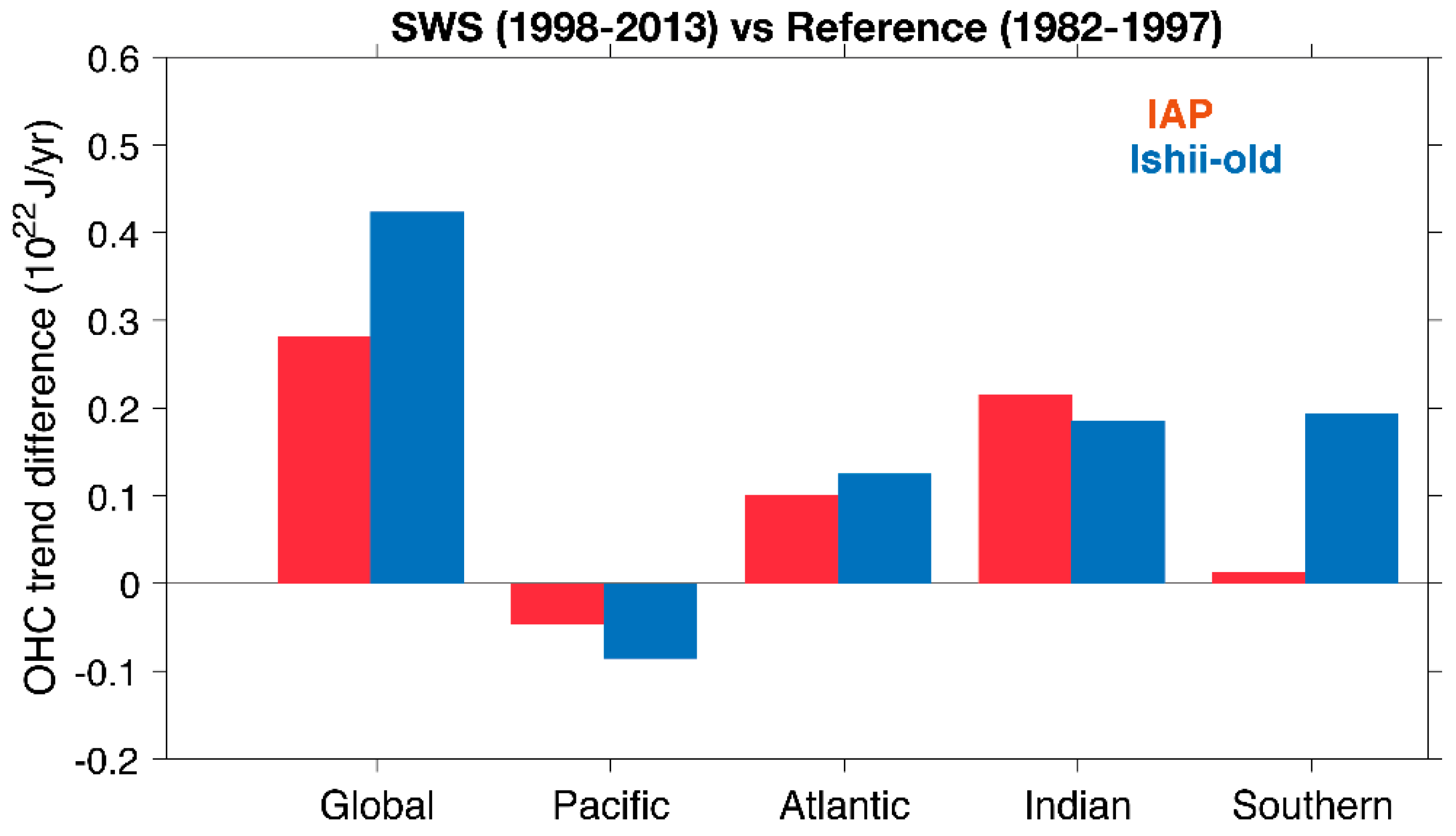
3.2. Observed Regional OHC Changes

First, it is imperative to clarify where the heat has been deposited during the SWS period (e.g., the spatial pattern). Figure 5 shows the geographical distribution of the temperature trend difference during the SWS period (1998–2013) compared with the reference period. Trend differences on the latitude-depth, longitude-depth, and latitude-longitude planes are plotted together to provide a 3-D illustration of the ocean interior changes. It is apparent that there was more heat deposited in the tropical and subtropical Western Pacific Ocean (20° S~20° N), the entire Indian Ocean (30° S~25° N), the North Atlantic Ocean (40° N~70° N), and the Tropical/South Atlantic (60° S~0) (Figure 5). The “hot spots” in the Western Pacific and Indian oceans are mainly located at ocean subsurface within 50–500 m, with a maximum at ~100 m in the Indian Ocean and 100~200 m in the Western Pacific Ocean, corresponding to the locations of the main thermocline. At the same time, the Eastern Pacific cooled. This contrasting west–east change in the Pacific Ocean implies a strengthening of the trade winds which leads to steepening tilt of the main thermocline in the tropical Pacific [4,38]. The stronger trade winds in the Pacific Ocean increase the Indonesian Through Flow (ITF), which transports warmer water in the Western Pacific into the Indian Ocean, primarily responsible for the Indian Ocean warming shown in Figure 4 and Figure 5 and other published studies [42,80]. Significant heating in the Indo-Pacific regions has also been found and explained in previous studies [32,42,62].
More heating in the Tropical/South Atlantic Ocean has not been extensively studied, but McGregor et al. [81] and Li et al. [82] hypothesized that the warming Atlantic Ocean is a major driver of the Pacific and Indian Ocean changes during the SWS period. Specifically, the AMO switched to a positive phase since the late 1990s, this resulted in the warming of the North Atlantic SST, which drives easterly wind anomalies over the Indo-Western Pacific through Kelvin waves and westerly anomalies over the eastern Pacific as Rossby waves [81,82].
In the North Atlantic, OHC sustained increases, which has been attributed primarily to the AMO [83,84,85]. Liu et al. [40] shows that the timing of the Atlantic Meridional Overturning Circulation (AMOC) change is not consistent with surface warming slowdown, since the AMOC weakened since mid-2000s while global surface warming was still paused.
Although there is a strong warming in the North Atlantic Ocean within 40° N~60° N, the “cold spots” in the broad areas in the North Pacific (20° N~60° N) and Atlantic Ocean (20° N~40° N) result in the lack of warming in the overall OHC changes in the Northern Hemisphere, also shown in Roemmich et al. [30] and Wijffels et al. [86] using Argo data.
The OHC changes in the Southern Ocean (60° S~30° S) in the SWS period are not as dramatic as other regions (Figure 4 and Figure 5), contradicting the claims in Chen and Tung [39] who showed more warming in the North Atlantic and Southern Oceans. That is because Chen and Tung [39] focused on the total OHC changes since 1998, and here we examine the difference between the 1998–2013 and the 1983–1997 periods. Therefore, implicitly, Chen and Tung [39] assumed that all of the OHC changes after 1998 are related to the SWS. However, as discussed earlier in this paper and many other studies [9,50,77], the Southern Ocean was experiencing a significant warming since 1960 due mainly to anthropogenic forcing, which was not related to the SWS. Therefore, one has to remove or reduce the influence of anthropogenic forcing when attributing the driver of the SWS. Our study used the trend difference between the 1998–2013 and 1983–1997 periods, Liu et al. [32] used models and also composite analysis to compare the warming “hiatus” and “acceleration” periods. While these methods are viable, it appears that Chen and Tung [39] failed to utilize them.
To give an idea of the long-term OHC changes caused by the anthropogenic forcing, Figure 6 presents the long-term ocean temperature trends from 1955 to 2017 to minimize the impact of inter-annual and decadal scale fluctuations in the OHC record. A distinct long-term ocean heating pattern was found and compared with the changes in the SWS period (comparing Figure 6 with Figure 5). The most prominent feature is the warming among almost the entire global ocean down to 2000 m with stronger warming near the surface than the deeper ocean (increased stratification). Some intriguing patterns emerge: stronger warming in the Southern Ocean (70° S~40° S) and North Atlantic Ocean (20° N~60° N) than the other regions; weaker warming in the entire Pacific and Indian Ocean (30° S~60° N). The long-term warming in the Southern Ocean has been identified and attributed primarily to greenhouse gasses (GHG) and ozone changes play a secondary role [50,76,77,87]. This warming in the Southern Ocean is almost the same for the 1998–2013 and 1982–1997 periods resulting in less significant changes for the trend differences shown in Figure 4.
In summary, regional OHC changes during the SWS period are examined and several “hot spots” and “cold spots” are identified and linked to previous literature. We show a significant ocean heat redistribution during the SWS period, which is distinct from the long-term ocean warming trend pattern. However, occurrences of the ocean “hot spots” or “cold spots” do not directly identify the key regions associated with the “driver” of the SWS. We will use regression analysis next to examine the possible linkage between surface changes and OHC, and give implications to the driver(s) of the ocean heat redistribution.

3.3. OHC Heat Redistribution Linked to Surface Decadal Modes

As indicated in the preceding section, several questions remain related to the oceanic heat redistribution. For instance, what mechanisms are responsible for the heat redistribution? Also, how could the major modes of climate variability impact the OHC patterns? Models might be the primary tool to fully disentangle these questions by separating the individual drivers, i.e., “pacemaker experiments” [4]. Considering the model errors, observation-based analyses can complement and provide a basis for model evaluation. In this section, we calculate linear regressions between the key indices of the surface temperature variability and the regional OHC changes in order to explore the OHC fingerprints of the major surface variability. The climate modes examined in this study include El Niño-Southern Oscillation (ENSO), PDO, and AMO, which are shown in Figure 7.

3.3.1. ENSO

ENSO is the strongest inter-annual perturbation to the climate system [88]. It has been argued that the changes in the frequency of different episodes of ENSO might be responsible for the SWS: there were more La Niña events during 2005–2013 and more El Niño events during 1998–2004 including an extreme 1997/98 event [89] (Figure 7). After removing ENSO’s impact from the GMST, the SWS disappears [34]. Cheng et al. [90] investigated the OHC changes related to ENSO, showing that the major OHC changes happen in the tropics including both adiabatic changes associated with the heat redistribution within the ocean at upper 300 m and diabatic changes associated with the heat loss in the tropical Pacific Ocean and gain in the tropical Atlantic/Indian Oceans.
Figure 8 shows geographical patterns of OHC trends, and its relationship to various indices. Figure 8b provides the regression between local OHC and an ENSO index (ONI: surface temperature in the Niño 3.4 region). A major feature of ENSO-related OHC change is the west-east seesaw pattern in the Pacific and Indian Oceans, with maximum cooling near the equator in the Eastern Pacific and maximum warming in the subtropical western Pacific Ocean. This relates to the change of the Pacific trade winds during ENSO and the associated thermocline tilt [90,91]. The ENSO-driven OHC changes in the Atlantic Ocean are very weak, with cooling within the 30° S~30° N region and warming in higher latitudes. Comparison between this ENSO-related pattern (Figure 8b) with the total SWS-OHC change (Figure 8a) shows some similarities in the Pacific Ocean, but a substantial difference outside of the Pacific Basin. The total SWS-OHC changes in the Western Pacific are generally consistent with ENSO-driven fingerprints: dramatic warming in the subtropical Western Pacific within 20° S~20° N and a cooling in the Northwest Pacific Ocean (20° N~40° N) and in coastal areas in the Northeast Pacific Ocean. However, the ocean cooling in the Eastern Pacific during the SWS period occurs outside of the equatorial areas, but ENSO-driven changes are near the equator. Also, SWS-OHC shows a broad warming within 30° S~30° N in both the Indian and Atlantic Oceans, but ENSO-driven pattern shows the opposite (Figure 8).

3.3.2. PDO

PDO (or IPO over the entire Pacific basin) is the leading hypothesis for the driver of the SWS period [2,3,4,38]. The PDO-related OHC patterns (Figure 8c) are broadly similar to the ENSO-driven patterns (Figure 8b), but with stronger signals in the middle- and high-latitudes. This is not surprising because PDO was sometimes interpreted as the low-frequency manifestation of the ENSO outside of the tropical bands [92]. A recent analysis based on model simulations show a broad similar PDO-related OHC pattern as identified by our observations [93].
PDO-driven patterns can broadly explain the SWS-OHC changes in the Pacific Ocean (seen by comparing Figure 8c and Figure 8a) and also in the North Atlantic Ocean (20° N~60° N). This provides OHC evidence for the important role of PDO in SWS. The strong PDO-driven OHC changes in the North Atlantic Ocean were related to the atmospheric teleconnections driven by the anomalous latent heating in the tropical Pacific Ocean [94].
However, in the Northwest Pacific Ocean (20° N–40° N), OHC during the SWS period shows a very strong cooling (Figure 4 and Figure 8a), but PDO-related cooling (Figure 8b) is very weak and confined within a much smaller area around ~20° N. In the Indian Ocean, PDO-driven OHC changes appear as a west-east seesaw pattern (similar to ENSO-driven pattern) and fail to explain the broad warming during the SWS period. In the tropical and subtropical Atlantic Ocean, the PDO is related to a broad ocean cooling (similar to ENSO), which is opposite to the SWS-OHC changes. Therefore, PDO cannot explain the SWS-OHC changes in these regions.

3.3.3. AMO

The North Atlantic has been hypothesized as the major driver of the SWS by Chen and Tung [39], which suggests that changes to the Atlantic Meridional Overturning Circulation play a key role. The AMO is often thought to be driven by the variability of the Atlantic Meridional Overturning Circulation (AMOC) [95]. Independent AMOC fingerprints derived from the observed subsurface ocean temperature indicate that the past AMOC variations are coherent with the observed AMO [96].
Figure 8d provides the regression between regional de-trended OHC changes with an AMO index. In the Atlantic Ocean from 30° S to 70° N, the AMO-driven changes are consistent with the SWS-OHC changes. This consistency suggests that, in addition to the PDO, the AMO might also be another mechanism in setting the Atlantic OHC patterns during the SWS period. In the Indian Ocean, AMO-driven patterns show a broad warming within 10° S to 30° N, similar to the SWS-OHC changes. Thus, the AMO provides the only mechanism among the three modes considered in this study to explain the Indian Ocean warming pattern; this supports the model-based study in Li et al. [82] suggesting an Atlantic driver of the global SST pattern during the SWS period.
In the Pacific Ocean, AMO can also drive an ocean cooling in the Eastern Pacific Ocean and warming in the Western Pacific Ocean (the maximum heating is located at Northwest Pacific at around 30° N). Therefore, AMO, PDO, and/or ENSO can all explain the Eastern Pacific cooling and Western Pacific heating pattern during the SWS period.
However, the AMO cannot explain the “cold spots” in the Northwest Pacific Ocean (20° N~40° N). Instead, AMO drives a strong warming trend in this region. In the Southern Ocean, AMO-driven patterns are generally opposite to SWS-OHC patterns, suggesting it is unlikely responsible for the Southern Ocean changes during the SWS period.

4. Discussion

Motivated by the debate related to the “global warming hiatus”, this study first suggests that it is a mistake to deny the “global warming” according to a slowing rate increase of GMST or SST over 13 years, despite the inability to find any statistically significant change in trends of these metrics. On the other hand, EEI and global OHC are fundamental metrics, as they indicate the radiative imbalance driven by GHG and they are less impacted by natural variability. Based on global OHC records, there is no indication of any pause in “global warming”, and in fact, the ocean warming is accelerating. Therefore, the term of “surface warming slowdown” was used in this study to clearly indicate any changing trend was unassociated with global warming. The scientific question then turns to: why is there a slowdown in GMST/SST with the continuous global warming and how are the GMST/SST changes related to ocean heat uptake?
On this basis, we reviewed the progress in OHC measurements and show the estimation error in traditional datasets could impact the identification of the ocean heat uptake. In this effort, a new dataset (IAP) was available for use. The most notable improvements in the new data are improved corrections for XBT bias, which significantly improvs the data quality; and a better mapping method, which effectively reduces the “conservative error” in previous dataset.
Based on the IAP data, complete 3-D temperature changes in the SWS period (related to the 1982–1997 period) in the ocean interiors are provided, with several “hot spots” and “cold spots” being identified. The decadal-scale ocean heat redistribution pattern is distinct from the long-term ocean heat uptake, confirming that natural variability dominates the decadal scale local OHC changes.
To give some implications on the driver of the ocean heat redistribution, we further perform a regression analysis to identify the OHC pattern related to three different climate models: ENSO, IPO, and AMO. The results indicate that none of them can solely explain the formation of the OHC patterns in the SWS period. Nevertheless, they can be important in different locations. The implication is that there might be no single answer to the occurrence of the SWS, instead, it is a combination of different phenomenon and different climate variability. Several model-based analyses also suggest that there are different flavors of the SWS period [8,97]. More analyses are required to investigate climate sensitivity and ocean heat uptake efficiency on decadal scales [98,99].

5. Concluding Remarks

Although this study attributes the SWS-related OHC change to natural variability, it does not relate it to the net EEI change in the climate system. Hedemann et al. [100] argued that SWS might be also caused by the reduction of EEI. Our results do not support this idea because the OHC increase (indicative of the EEI) has accelerated during the SWS period (Figure 1).
Furthermore, In Figure 1, it is apparent that the SWS ends with the appearance of the extreme 2015/16 El Niño event: the linear trend of GMST for 1998–2017 is 0.017 K/yr, larger than the linear trend during the reference (1982–1997) period (0.015 K/yr), also suggested in Hu et al. [101]. Loeb et al. [102] observed a shape increase of the net downward fluxes into the Earth system after 2014, more energy would support the further acceleration of the global warming.
This study also gives some implications for the future actions to understand the ocean heat uptake on different spatial and temporal scales:
(1).
The community should be clearer about the uncertainty in OHC. There are many lessons learned from the discrepancy of the different published analyses due to the uncertainty in OHC records. In the future, it will be helpful to quantify the signal versus error in OHC records at different temporal and spatial scales.
(2).
How do different climate modes impact the ocean heat uptake? Our observational analyses provide an ability to answer this question, but the caveat is that the record is still too short: i.e., the typical period of AMO and PDO is 30~70 years, similar to the length of the reliable OHC record (~60 years since the late 1950s). Combined analyses of models and observations are the proposed way forward.

Author Contributions

L.C. initiated this study, designed the experiments, and prepared figures and the first manuscript. G.W. contributed to preparation and analysis of the results. J.P.A. and G.H. contributed to refine the manuscript and analysis of the results.

Funding

This study is supported by National Key R&D Program of China (2017YFA0603202, 2018YFA0605904) and the National Natural Science Foundation of China (41506029, 41831175).

Acknowledgments

The authors thank the reviewers for their constructive comments. IAP data is available at http://159.226.119.60/cheng/.

Conflicts of Interest

The authors declare no conflict of interest. The funding sponsors had no role in the design of the study; in the collection, analysis, or interpretation of data; in the writing of the manuscript, and in the decision to publish the results.

References

  1. Hartmann, D.L.; Tank, A.M.G.K.; Rusticucci, M.; Alexander, L.V.; Brönnimann, S.; Charabi, Y.; Dentener, F.J.; Dlugokencky, E.J.; Easterling, D.R.; Kaplan, A.; et al. Observations: Atmosphere and surface. In Climate Change 2013: The Physical Science Basis. Contribution of Working Group I to the Fifth Assessment Report of the Intergovernmental Panel on Climate Change; Stocker, T.F., Qin, D., Plattner, G.-K., Tignor, M., Allen, S.K., Boschung, J., Nauels, A., Xia, Y., Bex, V., Midgley, P.M., Eds.; Cambridge University Press: Cambridge, UK; New York, NY, USA, 2013; pp. 159–254. [Google Scholar]
  2. Meehl, G.A.; Arblaster, J.M.; Fasullo, J.Y.; Hu, A.; Trenberth, K.E. Model-based evidence of deep-ocean heat uptake during surface-temperature hiatus periods. Nat. Clim. Chang. 2011, 1, 360–364. [Google Scholar] [CrossRef]
  3. Trenberth, K.E.; Fasullo, J.T. An apparent hiatus in global warming? Earth’s Future 2013, 1, 19–32. [Google Scholar] [CrossRef] [Green Version]
  4. Kosaka, Y.; Xie, S.-P. Recent global-warming hiatus tied to equatorial Pacific surface cooling. Nature 2013, 501, 403. [Google Scholar] [CrossRef] [PubMed]
  5. Fyfe, J.C.; Meehl, G.A.; England, M.H.; Mann, M.E.; Santer, B.D.; Flato, G.M.; Hawkins, E.; Gillett, N.P.; Xie, S.-P.; Kosaka, Y.; et al. Making sense of the early-2000s warming slowdown. Nat. Clim. Chang. 2016, 6, 224. [Google Scholar] [CrossRef]
  6. Yan, X.-H.; Boyer, T.; Trenberth, K.; Karl, T.R.; Xie, S.-P.; Nieves, V.; Tung, K.-K.; Roemmich, D. The global warming hiatus: Slowdown or redistribution? Earth’s Future 2016, 4, 472–482. [Google Scholar] [CrossRef] [Green Version]
  7. Held, I.M. CLIMATE SCIENCE The cause of the pause. Nature 2013, 501, 318–319. [Google Scholar] [CrossRef] [PubMed]
  8. Yao, S.-L.; Luo, J.-J.; Huang, G.; Wang, P. Distinct global warming rates tied to multiple ocean surface temperature changes. Nat. Clim. Chang. 2017, 7, 486. [Google Scholar] [CrossRef]
  9. IPCC. Climate Change 2013: The Physical Science Basis. In Intergovernmental Panel on Climate Change; Stocker, T.F., Ed.; Cambridge University Press: Cambridge, UK, 2013. [Google Scholar]
  10. USGCRP. Climate Science Special Report: Fourth National Climate Assessment, Volume I; Wuebbles, D.J., Fahey, D.W., Hibbard, K.A., Dokken, D.J., Stewart, B.C., Maycock, T.K., Eds.; U.S. Global Change Research Program: Washington, DC, USA, 2017; 470p. [Google Scholar]
  11. Karl, T.R.; Arguez, A.; Huang, B.; Lawrimore, J.H.; McMahon, J.R.; Menne, M.J.; Peterson, T.C.; Vose, R.S.; Zhang, H.-M. Possible artifacts of data biases in the recent global surface warming hiatus. Science 2015, 348, 1469–1472. [Google Scholar] [CrossRef] [PubMed] [Green Version]
  12. Foster, G.; Abraham, J. Lack of evidence for a slowdown in global temperature. US Clim. Var. Predict. Program 2015, 13, 6–9. [Google Scholar]
  13. Niamh, C.; Stefan, R.; Andrew, C.P. Change points of global temperature. Environ. Res. Lett. 2015, 10, 084002. [Google Scholar] [Green Version]
  14. Lewandowsky, S.; Risbey, J.S.; Oreskes, N. The “Pause” in Global Warming: Turning a Routine Fluctuation into a Problem for Science. Bull. Am. Meteorol. Soc. 2016, 97, 723–733. [Google Scholar] [CrossRef] [Green Version]
  15. Lewandowsky, S.; Risbey, J.S.; Oreskes, N. On the definition and identifiability of the alleged “hiatus” in global warming. Sci. Rep. 2015, 5, 16784. [Google Scholar] [CrossRef] [PubMed] [Green Version]
  16. Medhaug, I.; Stolpe, M.B.; Fischer, E.M.; Knutti, R. Reconciling controversies about the ‘global warming hiatus’. Nature 2017, 545, 41. [Google Scholar] [CrossRef] [PubMed]
  17. Hansen, J.; Sato, M.; Kharecha, P.; von Schuckmann, K. Earth’s energy imbalance and implications. Atmos. Chem. Phys. 2011, 11, 13421–13449. [Google Scholar] [CrossRef] [Green Version]
  18. Trenberth, K.; Fasullo, J.; Balmaseda, M. Earth’s Energy Imbalance. J. Clim. 2014, 27, 3129–3144. [Google Scholar] [CrossRef]
  19. Mann, M.E.; Zhang, Z.; Hughes, M.K.; Bradley, R.S.; Miller, S.K.; Rutherford, S.; Ni, F. Proxy-based reconstructions of hemispheric and global surface temperature variations over the past two millennia. Proc. Natl. Acad. Sci. USA 2008, 105, 13252–13257. [Google Scholar] [CrossRef] [PubMed] [Green Version]
  20. Johnson, G.C.; Lyman, J.M.; Boyer, T.; Cheng, L.; Domingues, C.M.; Gilson, J.; Ishii, M.; Killick, R.; Monselan, D.; Wijffels, S. Ocean heat content. In State of the Climate in 2017, Global Oceans. Bull. Am. Meteorol. Soc. 2018, 99, S72–S77. [Google Scholar]
  21. Nerem, R.S.; Beckley, B.D.; Fasullo, J.T.; Hamlington, B.D.; Masters, D.; Mitchum, G.T. Climate-change–driven accelerated sea-level rise detected in the altimeter era. Proc. Natl. Acad. Sci. USA 2018, 115, 2022–2025. [Google Scholar] [CrossRef] [PubMed] [Green Version]
  22. Shepherd, A.; Ivins, E.R.; Geruo, A.; Barletta, V.R.; Bentley, M.J.; Bettadpur, S.; Briggs, K.H.; Bromwich, D.H.; Forsberg, R.; Galin, N.; et al. A Reconciled Estimate of Ice-Sheet Mass Balance. Science 2012, 338, 1183–1189. [Google Scholar] [CrossRef] [PubMed] [Green Version]
  23. Durack, P.; Wijffels, S.E.; Matear, R.J. Ocean Salinities Reveal Strong Global Water Cycle Intensification During 1950 to 2000. Science 2012, 336, 455. [Google Scholar] [CrossRef] [PubMed]
  24. Rahmstorf, S.; Box, J.; Feulner, G.; Mann, M.; Robinson, A.; Rutherford, S.; Schaffernicht, E. Exceptional twentieth-Century slowdown in Atlantic Ocean overturning circulation. Nat. Clim. Chang. 2015, 5, 475–480. [Google Scholar] [CrossRef] [Green Version]
  25. Trenberth, K.E.; Cheng, L.; Jacobs, P.; Zhang, Y.; Fasullo, J. Hurricane Harvey Links to Ocean Heat Content and Climate Change Adaptation. Earth’s Future 2018, 6, 730–744. [Google Scholar] [CrossRef]
  26. Rhein, M.; Rintoul, S.R.; Aoki, S.; Campos, E.; Chambers, D.; Feely, R.A.; Gulev, S.; Johnson, G.C.; Josey, S.A.; Kostianoy, A.; et al. Observations: Ocean. In Climate Change 2013: The Physical Science Basis. Contribution of Working Group I to the Fifth Assessment Report of the Intergovernmental Panel on Climate Change; Stocker, T.F., Qin, D., Plattner, G.-K., Tignor, M., Allen, S.K., Boschung, J., Nauels, A., Xia, Y., Bex, V., Midgley, P.M., Eds.; Cambridge University Press: Cambridge, UK; New York, NY, USA, 2013. [Google Scholar]
  27. Cheng, L.; Trenberth, K.E.; Fasullo, J.; Abraham, J.; Boyer, T.P.; Schuckmann, K.V.; Zhu, J. Taking the pulse of the planet. EOS 2018, 98, 14–15. [Google Scholar] [CrossRef]
  28. von Schuckmann, K.; Palmer, M.D.; Trenberth, K.E.; Cazenave, A.; Chambers, D.; Champollion, N.; Hansen, J.; Josey, S.A.; Loeb, N.; Mathieu, P.P.; et al. An imperative to monitor Earth’s energy imbalance. Nat. Clim. Chang. 2016, 6, 138–144. [Google Scholar] [CrossRef] [Green Version]
  29. Cheng, L.; Trenberth, K.; Fasullo, J.; Boyer, T.; Abraham, J.; Zhu, J. Improved estimates of ocean heat content from 1960–2015. Sci. Adv. 2017, 3, e1601545. [Google Scholar] [CrossRef] [PubMed]
  30. Roemmich, D.; Church, J.; Gilson, J.; Monselesan, D.; Sutton, P.; Wijffels, S. Unabated planetary warming and its ocean structure since 2006. Nat. Clim. Chang. 2015, 5, 240. [Google Scholar] [CrossRef]
  31. Balmaseda, M.A.; Trenberth, K.E.; Källén, E. Distinctive climate signals in reanalysis of global ocean heat content. Geophys. Res. Lett. 2013, 40, 1754–1759. [Google Scholar] [CrossRef] [Green Version]
  32. Liu, W.; Xie, S.-P.; Lu, J. Tracking ocean heat uptake during the surface warming hiatus. Nat. Commun. 2016, 7, 10926. [Google Scholar] [CrossRef] [PubMed] [Green Version]
  33. Gleckler, P.J.; Durack, P.J.; Stouffer, R.J.; Johnson, G.C.; Forest, C.E. Industrial-era global ocean heat uptake doubles in recent decades. Nat. Clim. Chang. 2016, 6, 394–398. [Google Scholar] [CrossRef]
  34. Foster, G.; Rahmstorf, S. Global temperature evolution 1979–2010. Environ. Res. Lett. 2011, 6, 044022. [Google Scholar] [CrossRef] [Green Version]
  35. Power, S.; Casey, T.; Folland, C.; Colman, A.; Mehta, V. Inter-decadal modulation of the impact of ENSO on Australia. Clim. Dyn. 1999, 15, 319–324. [Google Scholar] [CrossRef]
  36. Kushnir, Y. Interdecadal Variations in North Atlantic Sea Surface Temperature and Associated Atmospheric Conditions. J. Clim. 1994, 7, 141–157. [Google Scholar] [CrossRef] [Green Version]
  37. Yao, S.-L.; Huang, G.; Wu, R.; Qu, X. The global warming hiatus—A natural product of interactions of a secular warming trend and a multi-decadal oscillation. Theor. Appl. Climatol. 2016, 123, 349–360. [Google Scholar] [CrossRef]
  38. England, H.M.; McGregor, S.; Spence, P.; Meehl, G.A.; Timmermann, A.; Cai, W.; Gupta, A.S.; McPhaden, M.J.; Purich, A.; Santoso, A. Recent intensification of wind-driven circulation in the Pacific and the ongoing warming hiatus. Nat. Clim. Chang. 2014, 4, 222. [Google Scholar] [CrossRef]
  39. Chen, X.; Tung, K.K. Varying planetary heat sink led to global-warming slowdown and acceleration. Science 2014, 345, 897–903. [Google Scholar] [CrossRef] [PubMed]
  40. Liu, W.; Xie, S.-P. An Ocean View of the Global Surface Warming Hiatus. Oceanography 2018, 31. [Google Scholar] [CrossRef]
  41. Palmer, M.D.; McNeall, D.J. Internal variability of Earth’s energy budget simulated by CMIP5 climate models. Environ. Res. Lett. 2014, 9, 034016. [Google Scholar] [CrossRef] [Green Version]
  42. Lee, S.; Park, W.; Baringer, M.; Gordon, A.; Huber, B.; Liu, Y. Pacific origin of the abrupt increase in Indian Ocean heat content during the warming hiatus. Nat. Geosci. 2015, 8, 445–449. [Google Scholar] [CrossRef] [Green Version]
  43. Drijfhout, S.S.; Blaker, A.T.; Josey, S.A.; Nurser, A.J.G.; Sinha, B.; Balmaseda, M.A. Surface warming hiatus caused by increased heat uptake across multiple ocean basins. Geophys. Res. Lett. 2015, 41, 7868–7874. [Google Scholar] [CrossRef]
  44. Palmer, M.D.; Roberts, C.D.; Balmaseda, M.; Chang, Y.-S.; Chepurin, G.; Ferry, N.; Fujii, Y.; Good, S.A.; Guinehut, S.; Haines, K.; et al. Ocean heat content variability and change in an ensemble of ocean reanalyses. Clim. Dyn. 2015, 49, 909–930. [Google Scholar] [CrossRef] [Green Version]
  45. Wang, G.; Cheng, L.; Abraham, J.; Li, C. Consensuses and discrepancies of basin-scale ocean heat content changes in different ocean analyses. Clim. Dyn. 2017, 50, 2471–2487. [Google Scholar] [CrossRef] [Green Version]
  46. Cheng, L.; Abraham, J.; Goni, G.; Boyer, T.; Wijffels, S.; Cowley, R.; Gouretski, V.; Reseghetti, F.; Kizu, S.; Dong, S.; et al. XBT Science: Assessment of Instrumental Biases and Errors. Bull. Am. Meteorol. Soc. 2016, 97, 924–933. [Google Scholar]
  47. Ishii, M.; Fukuda, Y.; Hirahara, S.; Yasui, S.; Suzuki, T.; Sato, K. Accuracy of Global Upper Ocean Heat Content Estimation Expected from Present Observational Data Sets. SOLA 2017, 13, 163–167. [Google Scholar] [Green Version]
  48. Boyer, T.; Domingues, C.; Good, S.; Johnson, G.; Lyman, J.; Ishii, M.; Gourestki, V.; Bindoff, N.; Church, J.; Cowley, R.; et al. Sensitivity of Global Ocean Heat Content Estimates to Mapping Methods, XBT Bias Corrections, and Baseline Climatology. J. Clim. 2016, 29, 4817–4842. [Google Scholar] [CrossRef]
  49. Fasullo, J.T.; Nerem, R.S.; Hamlington, B. Is the detection of accelerated sea level rise imminent? Sci. Rep. 2016, 6, 31245. [Google Scholar] [CrossRef] [PubMed] [Green Version]
  50. Shi, J.-R.; Xie, S.-P.; Talley, L.D. Evolving Relative Importance of the Southern Ocean and North Atlantic in Anthropogenic Ocean Heat Uptake. J. Clim. 2018, 31, 7459–7479. [Google Scholar] [CrossRef]
  51. Maher, N.; Sen Gupta, A.; England, M.H. Drivers of decadal hiatus periods in the 20th and 21st centuries. Geophys. Res. Lett. 2014, 41, 5978–5986. [Google Scholar] [CrossRef] [Green Version]
  52. Gregory, J.M.; Bi, D.; Collier, M.A.; Dix, M.R.; Hirst, A.C.; Hu, A.; Huber, M.; Knutti, R.; Marsland, S.J.; Meinshausen, M.; et al. Climate models without preindustrial volcanic forcing underestimate historical ocean thermal expansion. Geophys. Res. Lett. 2013, 40, 1600–1604. [Google Scholar] [CrossRef] [Green Version]
  53. Thompson, D.W.J.; Solomon, S.; Kushner, P.J.; England, M.H.; Grise, K.M.; Karoly, D.J. Signatures of the Antarctic ozone hole in Southern Hemisphere surface climate change. Nat. Geosci. 2011, 4, 741. [Google Scholar] [CrossRef]
  54. Sen Gupta, A.; Jourdain, N.C.; Brown, J.N.; Monselesan, D. Climate Drift in the CMIP5 Models. J. Clim. 2013, 26, 8597–8615. [Google Scholar] [CrossRef]
  55. Mayer, M.; Fasullo, J.T.; Trenberth, K.E.; Haimberger, L. ENSO-driven energy budget perturbations in observations and CMIP models. Clim. Dyn. 2016, 47, 4009–4029. [Google Scholar] [CrossRef] [Green Version]
  56. Gastineau, G.; Friedman, A.R.; Khodri, M.; Vialard, J. Global ocean heat content redistribution during the 1998–2012 Interdecadal Pacific Oscillation negative phase. Clim. Dyn. 2018. [Google Scholar] [CrossRef]
  57. Cheng, L.; Zhu, J. Benefits of CMIP5 Multimodel Ensemble in Reconstructing Historical Ocean Subsurface Temperature Variations. J. Clim. 2016, 29, 5393–5416. [Google Scholar] [CrossRef]
  58. Abraham, J.P.; Baringer, M.; Bindoff, N.L.; Boyer, T.; Cheng, L.J.; Church, J.A.; Conroy, J.L.; Domingues, C.M.; Fasullo, J.T.; Gilson, J.; et al. A Review of Global Ocean Temperature Observations: Implications for Ocean Heat Content Estimates and Climate Change. Rev. Geophys. 2013, 51, 450–483. [Google Scholar] [CrossRef]
  59. Lyman, J.M.; Good, S.A.; Gouretski, V.V.; Ishii, M.; Johnson, G.C.; Palmer, M.D.; Smith, D.M.; Willis, J.K. Robust warming of the global upper ocean. Nature 2010, 465, 334–337. [Google Scholar] [CrossRef] [PubMed]
  60. Levitus, S.; Antonov, J.I.; Boyer, T.P.; Baranova, O.K.; Garcia, H.E.; Locarnini, R.A.; Mishonov, A.V.; Reagan, J.R.; Seidov, D.; Yarosh, E.S.; et al. World ocean heat content and thermosteric sea level change (0–2000 m), 1955–2010. Geophys. Res. Lett. 2012, 39. [Google Scholar] [CrossRef]
  61. Ishii, M.; Kimoto, M.; Kachi, M. Historical ocean subsurface temperature analysis with error estimates. Mon. Weather Rev. 2003, 131, 51–73. [Google Scholar] [CrossRef]
  62. Nieves, V.; Willis, J.K.; Patzert, W.C. Recent hiatus caused by decadal shift in Indo-Pacific heating. Science 2015, 349, 532–535. [Google Scholar] [CrossRef] [PubMed]
  63. Liu, W.; Xie, S.-P.; Lu, J. Correspondence: Reply to: ‘Correspondence: Variations in ocean heat uptake during the surface warming hiatus’. Nat. Commun. 2016, 7, 12542. [Google Scholar] [CrossRef] [PubMed] [Green Version]
  64. Chen, X.; Tung, K.-K. Correspondence: Variations in ocean heat uptake during the surface warming hiatus. Nat. Commun. 2016, 7, 12541. [Google Scholar] [CrossRef] [PubMed] [Green Version]
  65. Good, S.A.; Martin, M.J.; Rayner, N.A. EN4: Quality controlled ocean temperature and salinity profiles and monthly objective analyses with uncertainty estimates. J. Geophys. Res. Oceans 2013, 118, 6704–6716. [Google Scholar] [CrossRef] [Green Version]
  66. Trenberth, K.E.; Shea, D.J. Atlantic hurricanes and natural variability in 2005. Geophys. Res. Lett. 2006, 33. [Google Scholar] [CrossRef] [Green Version]
  67. Palmer, M.D.; Boyer, T.; Cowley, R.; Kizu, S.; Reseghetti, F.; Suzuki, T.; Thresher, A. An algorithm for classifying unknown expendable bathythermograph (XBT) instruments based on existing metadata. J. Atmos. Ocean. Tech. 2018, 35. [Google Scholar] [CrossRef]
  68. Ishii, M.; Kimoto, M. Reevaluation of historical ocean heat content variations with time-varying XBT and MBT depth bias corrections. J. Oceanogr. 2009, 65, 287–299. [Google Scholar] [CrossRef]
  69. Cheng, L.; Luo, H.; Boyer, T.; Cowley, R.; Abraham, J.; Gouretski, V.; Reseghetti, F.; Zhu, J. How well can we correct systematic errors in historical XBT data? J. Atmos. Ocean. Technol. 2018, 35, 1103–1125. [Google Scholar] [CrossRef]
  70. Cheng, L.; Zhu, J.; Cowley, R.; Boyer, T.; Wijffels, S. Time, Probe Type and Temperature Variable Bias Corrections to Historical Expendable Bathythermograph Observations. J. Atmos. Ocean. Technol. 2014, 31, 1793–1825. [Google Scholar] [CrossRef]
  71. Levitus, S.; Antonov, J.I.; Boyer, T.P.; Locarnini, R.A.; Garcia, H.E.; Mishonov, A.V. Global ocean heat content 1955-2008 in light of recently revealed instrumentation problems. Geophys. Res. Lett. 2009, 36, 471–478. [Google Scholar] [CrossRef]
  72. Gouretski, V.; Reseghetti, F. On depth and temperature biases in bathythermograph data: Development of a new correction scheme based on analysis of a global ocean database. Deep-Sea Res. Part I Oceanogr. Res. Pap. 2010, 57, 812–833. [Google Scholar] [CrossRef]
  73. Lyman, J.M.; Johnson, G.C. Estimating Annual Global Upper-Ocean Heat Content Anomalies despite Irregular In Situ Ocean Sampling. J. Clim. 2008, 21, 5629–5641. [Google Scholar] [CrossRef]
  74. Durack, P.; Gleckler, P.J.; Landerer, F.; Taylor, K.E. Quantifying underestimates of long-term upper-ocean warming. Nat. Clim. Chang. 2014, 4, 999–1005. [Google Scholar] [CrossRef]
  75. Cheng, L.; Zhu, J. Artifacts in variations of ocean heat content induced by the observation system changes. Geophys. Res. Lett. 2014, 20, 7276–7283. [Google Scholar] [CrossRef]
  76. Gille, S.T. Decadal-scale temperature trends in the Southern Hemisphere ocean. J. Clim. 2008, 21, 4749–4765. [Google Scholar] [CrossRef]
  77. Swart, N.C.; Gille, S.T.; Fyfe, J.C.; Gillett, N.P. Recent Southern Ocean warming and freshening driven by greenhouse gas emissions and ozone depletion. Nat. Geosci. 2018, 11, 836. [Google Scholar] [CrossRef]
  78. Frölicher, T.L.; Sarmiento, J.L.; Paynter, D.J.; Dunne, J.P.; Krasting, J.P.; Winton, M. Dominance of the Southern Ocean in Anthropogenic Carbon and Heat Uptake in CMIP5 Models. J. Clim. 2014, 28, 862–886. [Google Scholar] [CrossRef]
  79. Marshall, J.; Speer, K. Closure of the meridional overturning circulation through Southern Ocean upwelling. Nat. Geosci. 2012, 5, 171. [Google Scholar] [CrossRef]
  80. Li, Y.; Han, W.; Zhang, L. Enhanced Decadal Warming of the Southeast Indian Ocean During the Recent Global Surface Warming Slowdown. Geophys. Res. Lett. 2017, 44, 9876–9884. [Google Scholar] [CrossRef]
  81. McGregor, S.; Timmermann, A.; Stuecker, M.F.; England, M.H.; Merrifield, M.; Jin, F.-F.; Chikamoto, Y. Recent Walker circulation strengthening and Pacific cooling amplified by Atlantic warming. Nat. Clim. Chang. 2014, 4, 888. [Google Scholar] [CrossRef] [Green Version]
  82. Li, X.; Xie, S.-P.; Gille, S.T.; Yoo, C. Atlantic-induced pan-tropical climate change over the past three decades. Nat. Clim. Chang. 2015, 6, 275. [Google Scholar] [CrossRef]
  83. Robson, J.; Ortega, P.; Sutton, R. A reversal of climatic trends in the North Atlantic since 2005. Nat. Geosci. 2016, 9, 513–517. [Google Scholar] [CrossRef]
  84. Piecuch, C.G.; Ponte, R.M.; Little, C.M.; Buckley, M.W.; Fukumori, I. Mechanisms underlying recent decadal changes in subpolar North Atlantic Ocean heat content. J. Geophys. Res. Oceans 2017, 122, 7181–7197. [Google Scholar] [CrossRef]
  85. Jackson, L.C.; Peterson, K.A.; Roberts, C.D.; Wood, R.A. Recent slowing of Atlantic overturning circulation as a recovery from earlier strengthening. Nat. Geosci. 2016, 9, 518. [Google Scholar] [CrossRef]
  86. Wijffels, S.; Roemmich, D.; Monselesan, D.; Church, J.; Gilson, J. Ocean temperatures chronicle the ongoing warming of Earth. Nat. Clim. Chang. 2016, 6, 116. [Google Scholar] [CrossRef]
  87. Liu, W.; Lu, J.; Xie, S.-P.; Fedorov, A. Southern Ocean Heat Uptake, Redistribution, and Storage in a Warming Climate: The Role of Meridional Overturning Circulation. J. Clim. 2018, 31, 4727–4743. [Google Scholar] [CrossRef]
  88. Trenberth, K.; Caron, M.; Stepaniak, D.; Worley, S. Evolution of El Niño–Southern Oscillation and global atmospheric surface temperatures. J. Geophys. Res. Atmos. 2002, 107, AAC 5-1–AAC 5-17. [Google Scholar] [CrossRef]
  89. Cheng, L.; Zheng, F.; Zhu, J. Distinctive ocean interior changes during the recent warming slowdown. Sci. Rep. 2015, 5, 14346. [Google Scholar] [CrossRef] [PubMed] [Green Version]
  90. Cheng, L.; Trenberth, K.E.; Fasullo, J.T.; Mayer, M.; Balmaseda, M.A.; Zhu, J. Evolution of ocean heat content related to ENSO. J. Clim. 2018. submitted. [Google Scholar]
  91. McPhaden, M.J. Playing hide and seek with El Niño. Nat. Clim. Chang. 2015, 5, 791. [Google Scholar] [CrossRef]
  92. Newman, M.; Alexander, M.A.; Ault, T.R.; Cobb, K.M.; Deser, C.; Lorenzo, E.D.; Mantua, N.J.; Miller, A.J.; Minobe, S.; Nakamura, H.; et al. The Pacific Decadal Oscillation, Revisited. J. Clim. 2016, 29, 4399–4427. [Google Scholar] [CrossRef]
  93. Hu, Z.; Hu, A.; Hu, Y. Contributions of Interdecadal Pacific Oscillation and Atlantic Multidecadal Oscillation to Global Ocean Heat Content Distribution. J. Clim. 2018, 31, 1227–1244. [Google Scholar] [CrossRef]
  94. Trenberth, K.E.; Fasullo, J.T.; Branstator, G.; Phillips, A.S. Seasonal aspects of the recent pause in surface warming. Nat. Clim. Chang. 2014, 4, 911–916. [Google Scholar] [CrossRef]
  95. Delworth, T.L.; Mann, M.E. Observed and simulated multidecadal variability in the Northern Hemisphere. Clim. Dyn. 2000, 16, 661–676. [Google Scholar] [CrossRef]
  96. Zhang, R. Coherent surface-subsurface fingerprint of the Atlantic meridional overturning circulation. Geophys. Res. Lett. 2008, 35. [Google Scholar] [CrossRef] [Green Version]
  97. Känel, L.; Frölicher, T.L.; Gruber, N. Hiatus-like decades in the absence of equatorial Pacific cooling and accelerated global ocean heat uptake. Geophys. Res. Lett. 2017, 44, 7909–7918. [Google Scholar] [CrossRef]
  98. Watanabe, M.; Kamae, Y.; Yoshimori, M.; Oka, A.; Sato, M.; Ishii, M.; Mochizuki, T.; Kimoto, M. Strengthening of ocean heat uptake efficiency associated with the recent climate hiatus. Geophys. Res. Lett. 2013, 40, 3175–3179. [Google Scholar] [CrossRef] [Green Version]
  99. Xie, S.-P.; Kosaka, Y.; Okumura, Y.M. Distinct energy budgets for anthropogenic and natural changes during global warming hiatus. Nat. Geosci. 2015, 9, 29. [Google Scholar] [CrossRef]
  100. Hedemann, C.; Mauritsen, T.; Jungclaus, J.; Marotzke, J. The subtle origins of surface-warming hiatuses. Nat. Clim. Chang. 2017, 7, 336–339. [Google Scholar] [CrossRef]
  101. Hu, S.; Fedorov, A.V. The extreme El Niño of 2015–2016 and the end of global warming hiatus. Geophys. Res. Lett. 2017, 44, 3816–3824. [Google Scholar] [CrossRef]
  102. Loeb, N.; Thorsen, T.; Norris, J.; Wang, H.; Su, W. Changes in Earth’s Energy Budget during and after the “Pause” in Global Warming: An Observational Perspective. Climate 2018, 6, 62. [Google Scholar] [CrossRef]
Figure 1. Global mean surface temperature (GMST) (green solid) and OHC (0–2000 m, purple solid) time series since 1955 with monthly time series in light lines and 12-month running means in thick lines. The surface warming slowdown (SWS) period (16 years from 1998 to 2013) is shaded in red and the previous 16-year period (1982–1997) is marked by blue shading. The linear trends for the two records during the two periods are shown in dashed lines. GMST data is Goddard Institute for Space Studies (GISS) Surface Temperature Analysis (GISTEMP) available at (https://data.giss.nasa.gov/gistemp/).
Climate 06 00091 g001
Figure 2. Ocean heat content changes in the upper 2000-m (1966–2016) with three superior XBT bias correction schemes in solid lines: Levitus et al. [71] (L09), Gouretski and Reseghetii [72] (GR10), and CH14 based on IAP mapping. For comparison, time series for Ishii-old, Ishii-new, and EN4 are attached in dashed curves. Ishii-old data is for 0–1500 m and all other data are for 0–2000 m (note that OHC change within 1500–2000 m is very small and is not responsible for the distinction between Ishii-old and IAP). 12-month running means are applied to all time series.
Climate 06 00091 g002
Figure 3. Temperature difference between August 1971 and August 1994 revealed by Ishii-old, Ishii-new, EN4, and IAP data at the depth of 600 m. Distribution of the temperature observations at 600 m in August 1971 (purple) and August 1994 (grey) are shown in dots.
Climate 06 00091 g003
Figure 4. Trend difference of OHC over the global ocean and four major ocean basins during the SWS period related to the reference period (1982–1997). IAP data is shown in red and Ishii-old is shown in blue. The Southern oceans represent ocean areas within 70° S to 30° S.
Climate 06 00091 g004
Figure 5. Trend difference between the surface slowdown period (1998–2013) and the 1982–1997 period. The front section shows the meridional mean temperature trend over the global ocean, the right section shows the zonal mean temperature trend. The upper map shows the trend of average temperature in the upper 2000 m range. IAP data is used. The units are K/yr.
Climate 06 00091 g005
Figure 6. Long-term ocean temperature trend since 1955. The front section shows the meridional mean temperature trend over the global ocean, the right section shows the zonal mean temperature trend. The upper map shows the trend of average temperature in the upper 2000 m range. IAP data is used. The units are K/yr.
Climate 06 00091 g006
Figure 7. Key indices of climate variability. El Niño-Southern Oscillation (ENSO) index: sea surface temperature in Nino 3.4 region, shown in as Oceanic Niño Index (ONI)—Niño (http://origin.cpc.ncep.noaa.gov/products/analysis_monitoring/ensostuff/ONI_v5.php); Pacific Decadal Oscillation (PDO) (https://www.esrl.noaa.gov/psd/gcos_wgsp/Timeseries/PDO/); and Atlantic Multi-decadal Oscillation (AMO) (https://www.esrl.noaa.gov/psd/data/timeseries/AMO/).
Climate 06 00091 g007
Figure 8. OHC 0–2000 m trend difference between the SWS period and reference period (a), similar to the top panel in Figure 5. OHC changes regressed onto the ENSO index (ONI) (b), PDO index (c), and AMO index (d). For ENSO/PDO, the negative regression coefficients are shown, because both ENSO and PDO are shifted to the negative phase (more La Nina episode for ENSO) during the SWS period. For OHC, a linear trend is removed before the regression is calculated, and the insignificant regression coefficients (at 95% confidence interval) are stippled.
Climate 06 00091 g008

