Article

Estimating the Impact of Artificially Injected Stratospheric Aerosols on the Global Mean Surface Temperature in the 21th Century

by
Sergei A. Soldatenko
St. Petersburg Institute for Informatics and Automation of the Russian Academy of Sciences, No. 39, 14-th Line, St. Petersburg 199178, Russia
Climate 2018, 6(4), 85; https://doi.org/10.3390/cli6040085
Submission received: 28 September 2018 / Revised: 24 October 2018 / Accepted: 26 October 2018 / Published: 28 October 2018
(This article belongs to the Special Issue Climate Variability and Change in the 21th Century)

Abstract

:
In this paper, we apply the optimal control theory to obtain the analytic solutions of the two-component globally averaged energy balance model in order to estimate the influence of solar radiation management (SRM) operations on the global mean surface temperature in the 21st century. It is assumed that SRM is executed via injection of sulfur aerosols into the stratosphere to limit the global temperature increase in the year 2100 by 1.5 °C and keeping global temperature over the specified period (2020–2100) within 2 °C as required by the Paris climate agreement. The radiative forcing produced by the rise in the atmospheric concentrations of greenhouse gases is defined by the Representative Concentration Pathways and the 1pctCO2 (1% per year CO2 increase) scenario. The goal of SRM is formulated in terms of extremal problem, which entails finding a control function (the albedo of aerosol layer) that minimizes the amount of aerosols injected into the upper atmosphere to satisfy the Paris climate target. For each climate change scenario, the optimal albedo of the aerosol layer and the corresponding global mean surface temperature changes were obtained. In addition, the aerosol emission rates required to create an aerosol cloud with optimal optical properties were calculated.

1. Introduction

Climate change is among the most significant threats to human civilization in the 21st century and beyond [1]. The Paris Climate Accord proposed to hold average temperature increase “to well below 2 °C above pre-industrial levels” and to pursue efforts to keep warming “below 1.5 °C above pre-industrial levels” [2]. To reach these goals, eight countries have already presented long-term low-emission strategies, which aims to reduce greenhouse gas emissions; several countries are currently in the process of preparing such strategies [3]. Meanwhile, the World Meteorological Organization’s (WMO) “Statement of the State of the Global Climate in 2017” released in January 2018 said, “The global mean temperature in 2017 was approximately 1.1 °C above the pre-industrial era” [4]. There is high confidence that planetary warming will continue throughout the 21st century even if we immediately stopped emitting greenhouse gases into the atmosphere (e.g., References [5,6,7,8,9]). Some resent studies (e.g., References [10,11,12,13]) suggest that geoengineering technologies can serve as a supplementary measure to stabilize climate as “in the absence of external cooling influence” [14], it is hard to achieve the Paris Agreement climate goals.
Solar radiation management (SRM) by injection of sulfur aerosols into the stratosphere [15,16] is one of the most feasible and promising solutions for inducing negative radiative forcing (RF) from aerosols in order to at least partially compensate the positive RF from atmospheric greenhouse gases. The current state of understanding of climate engineering technologies, including SRM, has been discussed in References [17,18,19,20,21,22,23,24,25,26]. Over the years, climate models have played a key role in exploring geoengineering techniques and predicting and quantifying their potential effects on Earth’s climate (e.g., References [27,28,29,30,31,32,33,34,35,36]). Due to the uncertainties inherent in climate models that could not be sufficiently reduced over the last decade [37], the resulting range of possible outcomes of hypothetical geoengineering efforts remains quite vague. To handle the climate response uncertainties, some studies (e.g., References [38,39,40,41,42,43,44,45]) have suggested modeling the Earth’s climate as a control system with feedbacks, which allows planning scenarios for geoengineering using the so-called “design model”. This formulation makes it possible to design the control law and calculate the amount of SRM forcing as a function of time needed to offset the rise in global mean surface temperature due to human-caused positive RF. Meanwhile, exploring Earth’s global climate as controlled dynamical system, we can approach geoengineering from the perspective of optimal control theory [46,47,48,49]. Within the optimal control framework, the goal of geoengineering can be formulated in terms of extremal problem, which involves finding control functions and the corresponding climate system trajectory that minimize or maximize a certain objective functional (also referred to as performance measure or index) subject to various constraints (e.g., References [50,51]. If x is the state vector of climate system and u is the vector of control variables, then the abstract extremal problem can be formulated as follows:
  J ( x , u ) e x t r ,     F ( x ,   u ) = 0 ,     ( x ,   u ) M X × U  
The statement of this problem includes a set X × U on which the (real) functional J ( x , u ) is defined and constraints imposed on state and control variables given by the model of control object F ( x ,   u ) = 0 (dynamic constraints) and by the subset M in X × U . The solution to the extremal problem (Equation (1)) is the optimal process ( x , u ) . Thus, by solving the optimal control problem (OCP), we can obtain the mathematically rigorous control law and the corresponding system’s trajectory that are relevant for the specified performance measure J ( x , u ) .
This paper deals with a simple mathematical model for controlling the global mean surface temperature T s f c in the 21st century by the injection of sulfur aerosols into the stratosphere to limit the global temperature increase in the year 2100 by 1.5 °C above pre-industrial level and keeping global temperature over the period of 2020–2100 within 2 °C as required by the Paris climate agreement. The objective is to minimize resources (the total mass of aerosols) required to achieve the desired final state of the climate system. In the model, the positive RF produced by the rise in the atmospheric concentrations of greenhouse gases is specified in accordance with the Representative Concentration Pathways [52] and the 1pctCO2 (1% per year CO2 increase) scenario.
The mathematical statement of OCP is the collection of the following key elements: objective function defined to judge the effectiveness of control process, mathematical model of the controlled object, equality and inequality constraints to be satisfied by state and control variables, and boundary and initial conditions (if any) for state variables. To imitate the behavior of the climate system, we applied a two-component energy balance model [53,54,55] in which the global mean surface temperature anomaly (perturbation) represents the variable that interests us the most, and the albedo of the global aerosol layer is designated as the control variable. We derived analytical expressions for both the optimal albedo of the global aerosol layer and the corresponding change in the global mean surface temperature.
The results of illustrative calculations are presented for the period 2020–2100. For each climate change scenario, the optimal albedo of the aerosol layer—and therefore the aerosol emission rates—as well as the associated global mean surface temperature changes were found.
We need to emphasize that the main reason for using such a model is that similar two-layer models have been considered and analyzed in a number of papers considering the response to forced climate change. For example, Geoffroy et al. [56,57] obtained and discussed the general analytical solutions of the two-layer model for different hypothetical climate forcing scenarios and suggested the approach of calibrating the model parameters to imitate the time response of coupled general circulation models (CGCMs) from CMIP5 to radiative forcing. Gregory et al. [58] analyzed the two-layer model and discussed the transient climate response, the global mean surface air temperature change under two scenarios: one with a step forcing (the abrupt 4xCO2 experiment) and one with the 1pctCO2 scenario. Despite the fact that the two-layer model is one of the simplest tools to mimic climate dynamics under external radiative forcing, it was able to simulate the evolution of average global surface temperature over time in response to both abrupt and time-dependent forcing with reasonable accuracy (e.g., References [56,59]).
In the two-layer model, climate control is carried out via changing Earth’s planetary albedo by injection of sulfur aerosols into the stratosphere (“albedo modification”). Sulfur aerosols increase the amount of sunlight that is scattered back to space, thereby reducing the amount of sunlight absorbed by Earth. Inherently, the planetary albedo is an average of the local albedo, averaged over the entire globe. The local albedo, in turn, is a highly variable dimensionless parameter that depends on a number of local factors, such as the composition of the atmosphere and in particular the presence of aerosols, the cloud amount and properties [60], the sea ice cover [61], the land use [62,63,64], the snow cover [65], etc. A typical value of Earth’s planetary albedo is about 0.3 [66].
As change in the albedo of our planet is a powerful driver of climate (indeed, a 1% change in the Earth’s planetary albedo generates the radiative effect of 3.42 Wm−2, which is commensurate with radiative forcing due to a doubling of CO2 concentrations in the atmosphere), scientists have proposed “albedo modification” as a powerful tool to deal with global warming (e.g., References [16,20,23,29,31,33,67]).

2. Materials and Methods

2.1. The Model of Control Object

The control object is Earth’s climate system. To simulate the climate system dynamics under the influence of external radiative forcing, we have applied the mathematical model consisting of two subsystems: One is the upper layer subsystem, which combines the atmosphere, the land surface, and the upper ocean; the other is the lower layer subsystem, which represents the deep ocean [53,54,55]. The state of each subsystem is characterized by the corresponding temperature perturbation (anomaly) with respect to initial climate “equilibrium” state. Denoting temperature anomalies for upper and lower subsystems by T and T D , respectively, the equations that govern these perturbations can be written as follows:
  C U d T d t = λ T γ ( T T D ) + Δ R CO 2 + ( 1 α 0 ) Δ R A  
  C D d T D d t = γ ( T T D )  
Here, C U and C D are the effective heat capacities of the upper and lower models, respectively (note that C U C D ); λ is a climate radiative feedback parameter; γ is a coupling strength parameter that describes the rate of heat loss by the upper layer; Δ R CO 2 is the radiative forcing caused by global increase in the atmospheric CO2 concentration; Δ R A is the negative radiative forcing generated by the artificial aerosols at the top of the atmosphere; and α 0 is Earth’s planetary albedo. We will assume that the temperature anomaly T is identified with the global mean surface temperature change T s f c [53,54].
Despite its simplicity, this model imitates climate changes under external radiative forcing with reasonable accuracy [56,57,58,59]. We have chosen values of 7.34   W   y r   m 2   K 1 , 105.5   W   y r   m 2   K 1 , 1.13   W   m 2   K 1 , and 0.7   W   m 2   K 1 for parameters C U ,     C D ,     λ , and γ , respectively. These values are taken in accordance with values consistent with the CMIP5 multimodel mean under climate change derived in Reference [56].
For convenience sake, we have rewritten the model Equations (2) and (3) as follows:
  d T d t = a T + b T D + Δ R CO 2 C U + ( 1 α 0 ) Δ R A C U  
  d T D d t = p T p T D  
where
  a = λ + γ C U ,       b = γ C U ,       p = γ C D .  
Ordinary Differential Equations (4) and (5) represent a mathematical model of the object to be controlled.

2.2. Parameterization of the Aerosols’ Radiative Effect

The climate control is assumed to be executed through the injection of nonabsorptive sulfate aerosols into the stratosphere. Injected aerosol particles scatter shortwave solar radiation back to the outer space and consequently change the radiative balance of our planet, increasing Earth’s planetary albedo and therefore causing the negative RF at the top of the atmosphere [68,69,70,71]:
  Δ R A = α A Q 0  
Here, α A is the instant albedo of the global aerosol layer; Q 0 is the global average incoming solar radiation on the top of the atmosphere defined as Q 0 = I 0 / 4 , where I 0 = 1368   W   m 2 is a solar constant [72,73]. Thus, to estimate the radiative effect of stratospheric aerosol, we need to calculate the albedo α A , which is considered as the control variable. However, in reality, we have the ability to manipulate the emission rate of aerosols injected into the stratosphere E A . To determine E A from the known α A , the mass balance equation is used:
  d M A d t = E A M A τ A  
where τ A is the residence time of stratospheric aerosol particles; M A is the global mass of the stratospheric aerosols, which is linearly related to the albedo α A [69]:
α A = M A ( β A k A / Q 0 S e )  
where the coefficient β A = 24 W m−2 [70,71]; k A = 7.6   m 2 g 1 is the mass extinction coefficient [69]; S e is Earth’s area determined as S e = 4 π R e 2 , where R e = 6371   km is Earth’s radius.
In geoengineering, sulfate aerosol particles are not directly injected into the stratosphere but can be formed from gaseous precursors, such as sulfur dioxide SO2, hydrogen sulfide H2S, carbonyl sulfide OCS, or dimethyl sulfide (DMS), which then convert into aerosols. We will express the emission rate of aerosol precursors as well as the mass of sulfate aerosols in units of sulfur, denoting them by E S (in Tg S yr−1) and M S (in Tg S), respectively. Assuming that 1 Tg of sulfur injected into the stratosphere forms approximately 4 Tg of aerosol particles [74], we obtain that E S E A / 4 and M S M A / 4 . As the relationship between M A and α A is linear, the following predictive equation for α A can be derived from Equation (8):
  d α A d t = χ 1 E S α A τ A  
where χ = Q 0 S e / ( 4 β A k A ) 2.39 × 10 2   Tg   S .
Thus, solving the OCP, we can find the optimal control law α A ( t ) and then calculate the optimal aerosol emission rate E S ( t ) using Equation (10).

2.3. Parameterization of the Anthropogenic Radiative Forcing

In energy balance models, simple empirical expressions are generally used to calculate radiative forcing due to the increase in atmospheric greenhouse gases. For example, the radiative forcing caused by a perturbation of the atmospheric burden of CO2 can be parameterized as a function of CO2 only [75,76]: Δ R CO 2 = κ × ln [ C CO 2 ( t ) / C CO 2 ( 0 ) ] , where κ (W m−2) is the empirical coefficient; C CO 2 ( t ) is the CO2 concentration at time t; and C CO 2 ( 0 ) is the reference CO2 concentration level. A typical value for the parameter κ is near 5.35 W m2 [75,76]. In our model, we have taken the total global mean anthropogenic and natural radiative forcing Δ R N as prescribed by the different scenarios and approximated by a linear function of time:
  Δ R N = η t  
where η is the annual rate of forcing (see Table 1).

2.4. Optimal Control Problem Formulation

We let [ t 0 ,   t f ] be a finite and fixed time interval. The OCP is defined as follows:
We find the control function α A ( t ) generating the corresponding temperature anomalies T ( t ) and T D ( t ) that minimizes the objective function:
  J = 1 2 t 0 t f α A 2 ( t ) d t  
subject to the dynamics (4) and (5) and given initial T ( t 0 ) = 0 and T D ( t 0 ) = 0 , as well as final (terminal) T ( t f ) = T f conditions.
In this formulation, the terminal condition T f is interpreted as a target change in the global mean surface temperature at t = t f , and the performance index (Equation (12)) characterizes the aerosol consumption for SRM operations (recall that α A and M A are linearly dependent functions). Thus, we wish to minimize the mass of aerosols required to reach the target surface temperature change at the final time. The global mean deep ocean temperature anomaly at the final time t f is not defined because changes in the global mean surface temperature are of primary concern, while changes in the deep ocean temperature are only of secondary concern. The total amount of aerosols annually emitted to the stratosphere can be limited by the available technical equipment. In this case, the minimization problem (Equation (12)) should be considered within the framework of control-constrained OCP. The set of admissible controls is given formally by α A [ 0 ,   U ] , where U is the maximum value of technically feasible and affordable albedo α A .

2.5. Method for Solving the Optimal Control Problem

Before proceeding further, we rewrite the model Equations (4) and (5) by replacing Δ R C O 2 with η t (11) and Δ R A with α A Q 0 (7):
  d T d t = a T + b T D + c t q α A  
  d T D d t = p T p T D  
where c = η / C U and q = ( 1 α 0 ) Q 0 / C U .
We solve the formulated OCP using the Pontryagin’s maximum principle (PMP) [47]. The Hamiltonian function for the problem (12) is defined as follows:
  H = 1 2 α A 2 + ψ 1 ( a T + b T D + c t q α A ) + ψ 2 ( p T p T D )  
where ψ 1 and ψ 2 are time-varying Lagrange multipliers, also known as costate or adjoint variables, which satisfy the adjoint system:
  d ψ 1 d t =   H T = a ψ 1 p ψ 2  
  d ψ 2 d t = H T D = b ψ 1 + p ψ 2  
The PMP states that the optimal control α A ( t ) [ 0 ,   U ] is one that would maximize the Hamiltonian (Equation (13)) at each fixed time t [ t 0 ,   t f ] :
  α A = arg   max α A [ 0 , U ] H ( α A )  
Therefore, to find the optimal control α A , we must maximize H with respect to α A , where the control belongs to the admissible control region α A [ 0 , U ] . The Hamiltonian maximization condition is as follows:
    H α A = α A q ψ 1 = 0  
Thus, to find the optimal control and the corresponding climate system’s trajectory, we need to solve the set of four ordinary Differential Equations (13), (14), (16), and (17) in four unknowns T , T D , ψ 1 , and ψ 2 with given initial and terminal conditions. As the variable T D is not defined at t f , the following transversality condition for costate variable ψ 2 applies: ψ 2 ( t f ) = 0 [48,49]. The analytic expressions derived for the control variable α A and temperature anomalies T and T D can be written as follows:
  α A ( t ) = C 1 q [ v 11 e λ 1 t + e ( λ 1 λ 2 ) t f v 21 e λ 2 t ]  
  T ( t ) = C 1 α 1 ( e λ 1 t e λ 2 t ) + C 3 e λ 1 t + C 4 e λ 2 t + + w 2 t + w 1  
  T D ( t ) = C 3 a λ 1 b e λ 1 t + C 4 a λ 2 b e λ 2 t +  
  + C 1 [ α 1 ( a + α 1 ) q 2 v 11 b e λ 1 t α 2 ( a + α 2 ) q 2 v 21 e ( λ 1 λ 2 ) t f b e λ 2 t ] +  
  + a w 2 c b t + a w 1 + w 2 b  
where C 1 , C 3 , and C 4 are arbitrary integration constants (note that the integration constant C 2 = C 1 e ( λ 1 λ 2 ) t f ); λ 1 and λ 2 are the eigenvalues of the coefficient matrix of the adjoint system, Equations (14) and (15); v 11 and v 21 are the components of the corresponding eigenvectors.
  α 1 = q 2 v 11 ( λ 1 + p ) λ 1 2 + λ 1 ( a + p ) + ( a p p b )  
  α 2 = q 2 v 21 ( λ 2 + p ) e ( λ 1 λ 2 ) t f λ 1 2 + λ 1 ( a + p ) + ( a p p b )  
  w 1 = c [ ( a p p b ) p ( a + p ) ] ( a p p b ) 2  
  w 2 = p c a p p b  
The constants of integration are determined by applying the boundary conditions.
If we consider climate engineering as a state-constrained OCP with constraints on the state variables, then additional necessary conditions for optimality, known as the complementary slackness conditions, should be specified [77]. In this study, we express the OCP with the following state constraint:
  T ( t ) C T               t [ t 0 ,   t f ]  
where C T is the threshold parameter whose value should be set. The meaning of the condition (Equation (23)) known as a path constraint is that throughout the geoengineering project, the global mean surface temperature change should not exceed a certain value C T , which is determined a priori. We should highlight that state constraints add a great deal of complexity to the OCP [77,78].

3. Results and Discussion
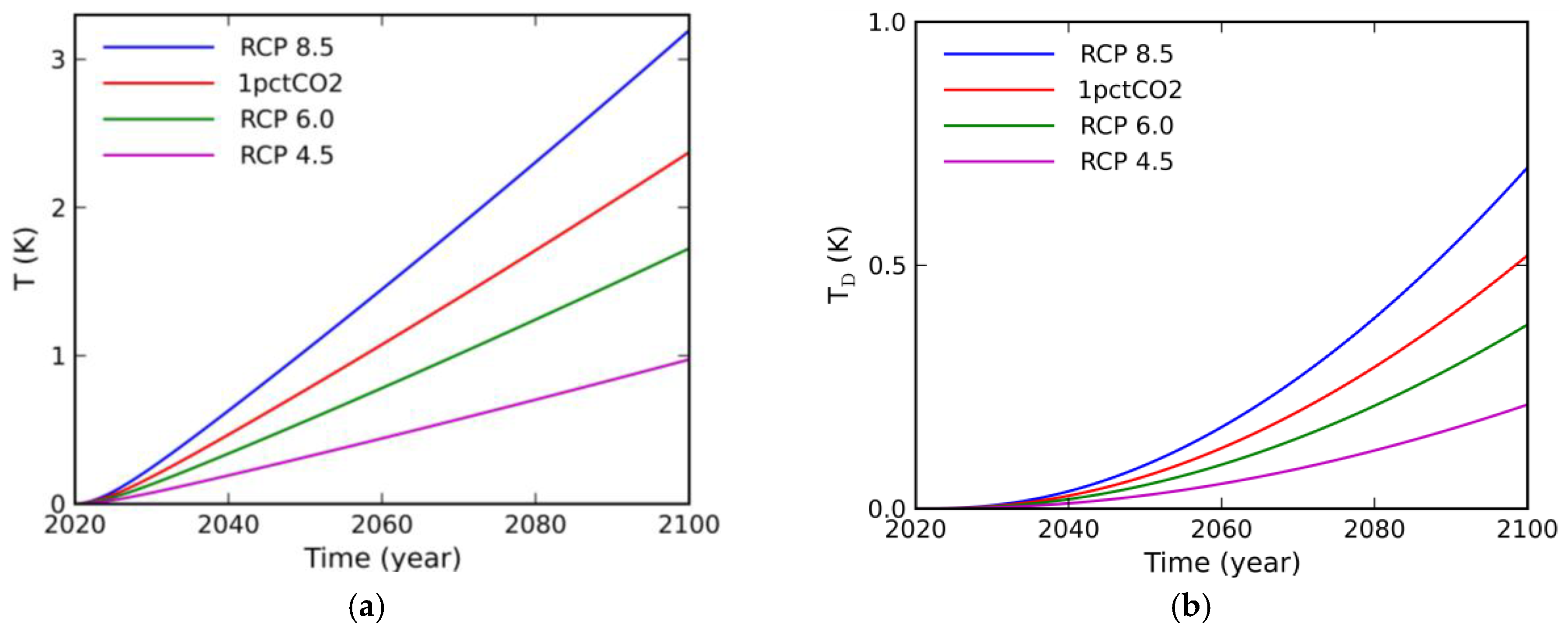
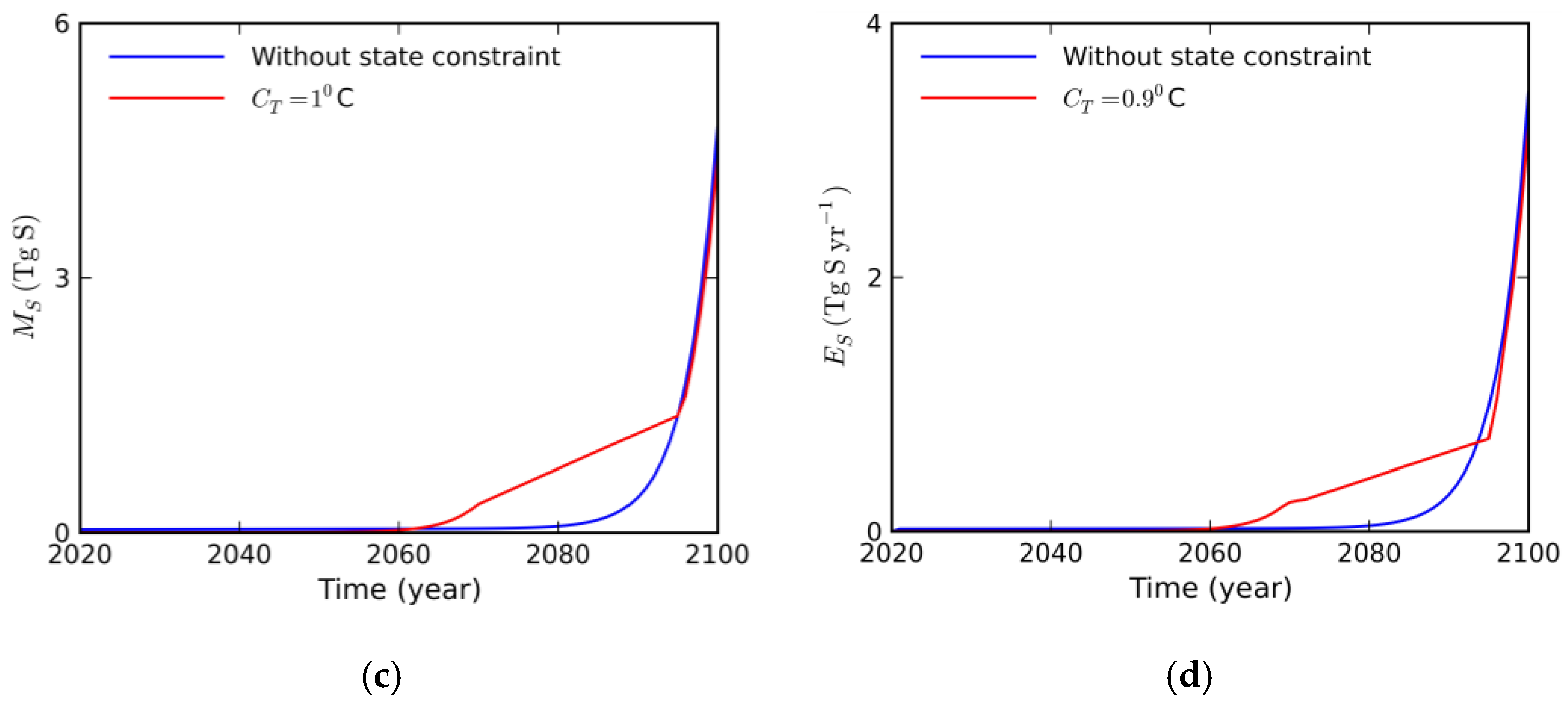
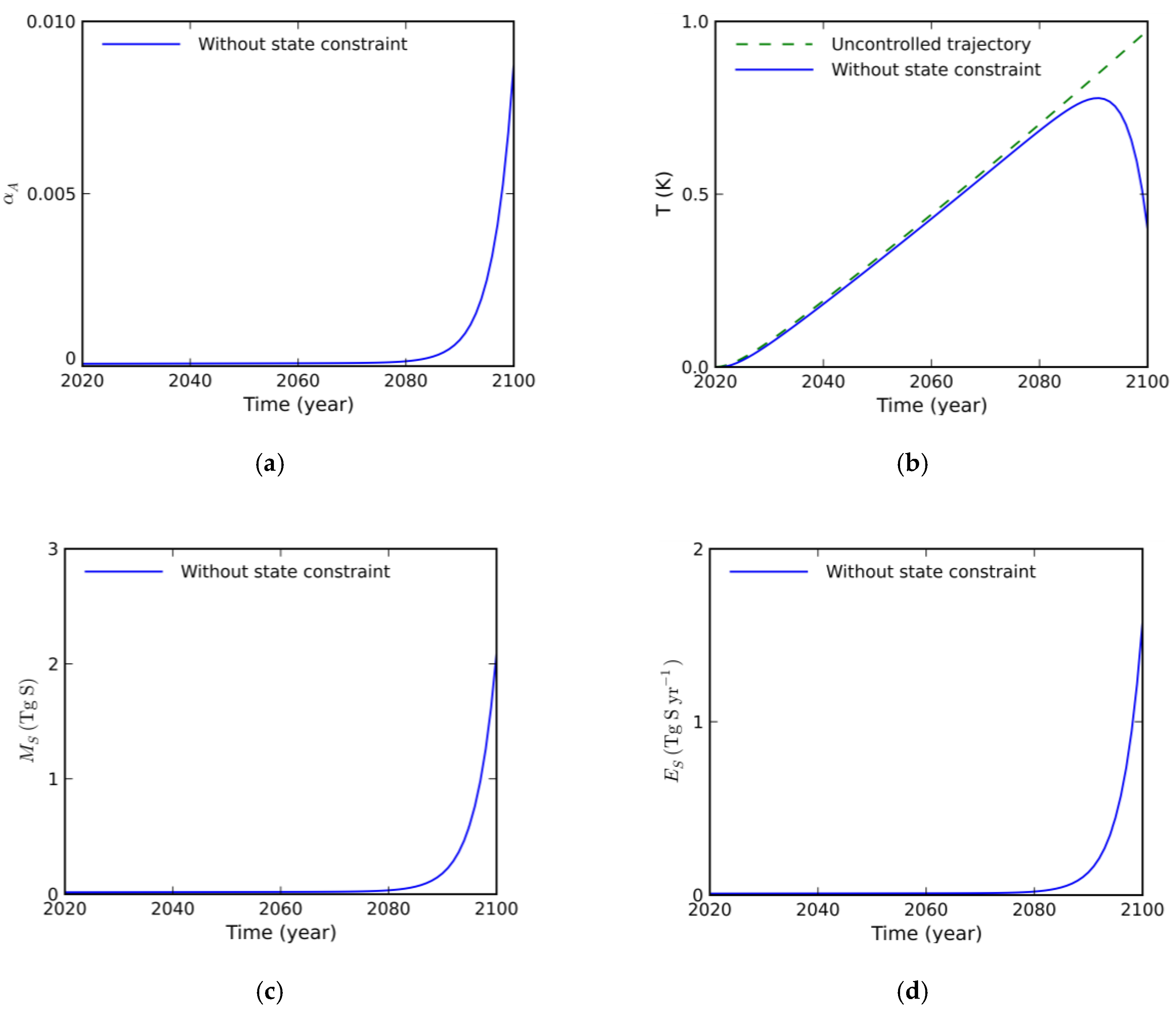
In the calculations, we took calendar years 2020 and 2100 as the initial t 0 and the final (terminal) t f time, respectively, which meant that we were examining the climate control problem on the finite time interval 2020–2100. To formulate the boundary conditions and impose a constraint on change in the global mean surface temperature T s f c , we assumed the following:
-
The temperature anomalies T and T D were calculated relative to 2020, i.e., the boundary conditions for T and T D at t = t 0 were T 2020 = 0 and T D ,   2020 = 0 , respectively, where the numerical subscript referred to the year 2020.
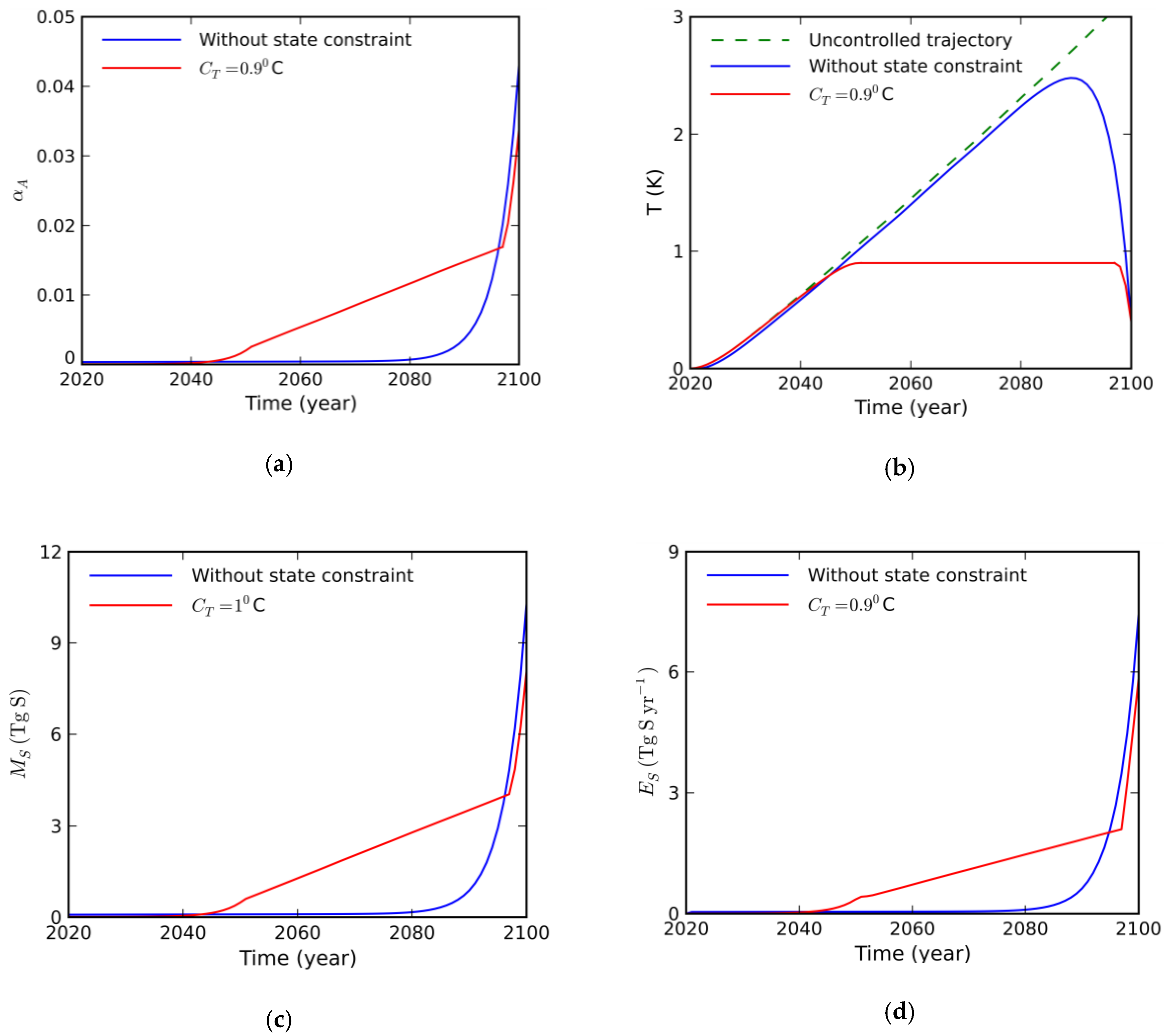
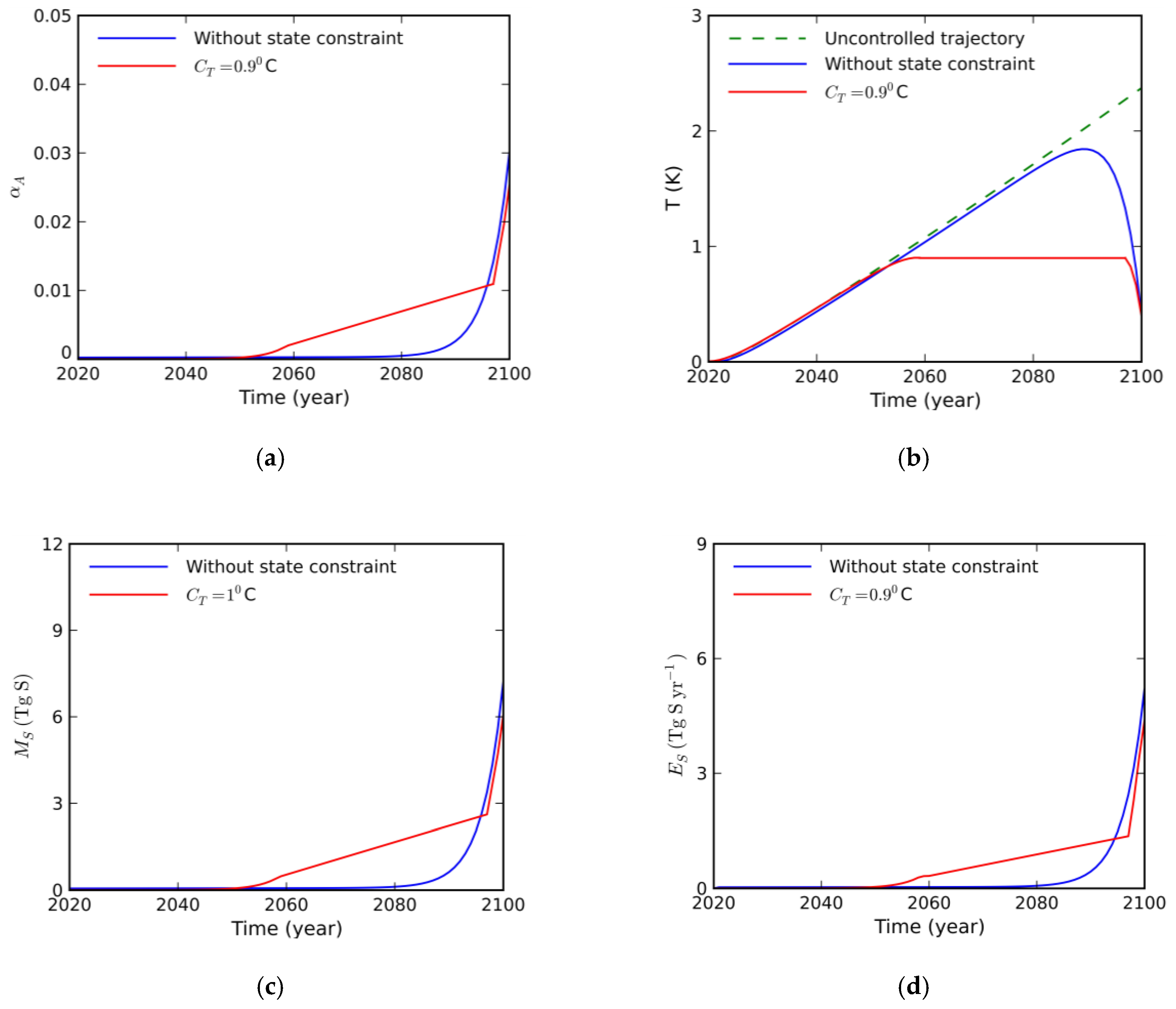
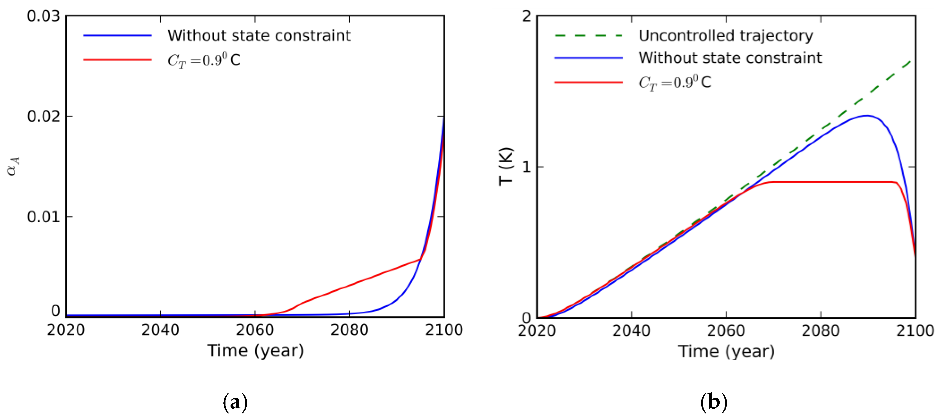
-
By 2020, T s f c would exceed the pre-industrial level by 1.1 °C, i.e., Δ T 2020 = 1.1   .
-
By 2100, T s f c would exceed the pre-industrial level by 1.5 °C, i.e., Δ T 2100 = 1.5   .
-
For the 2020 to 2100 period, the rise in T s f c should not exceed 2 °C above the pre-industrial level.
Then, the permissible increase in the temperature anomaly T 2100 by year 2100 relative to 2020 would be T 2100 = Δ T 2100 Δ T 2020 = 0.4   . This value represents the boundary condition for T at t = t f . The threshold parameter, which defines a path constraint (Equation (23)), is C T = 2   Δ T 2020 = 0.9   .
Changes in both global mean surface temperature and deep ocean temperature calculated for different climate change scenarios in the absence of climate engineering interventions are illustrated in Figure 1. The corresponding temperature changes in the year 2100 are shown in Table 2. According to Reference [79], without additional measures to reduce GHG emissions (RCP8.5 scenario), increases in global mean surface temperatures are expected to be between 3.7 and 4.8 °C by the year 2100 versus pre-industrial levels (this range is based on median climate response). As seen in Table 2, by year 2100, the model outlined here projects globally averaged surface temperature increases of 4.26, 3.44, and 2.80 °C for the RCP8.5, 1pctCO2, and RCP6.0 scenarios, respectively (relative to pre-industrial period). Thus, geoengineering can be regarded as one of supplementary measures needed to achieve the climate targets of the Paris Agreement.
We considered results of calculations for the RCP8.5 (the worst-case) scenario in more detail. Figure 2 shows (a) the optimal albedo of the global stratospheric aerosol layer, (b) the corresponding surface temperature anomaly, (c) the mass of the global aerosol layer, and (d) the optimal emission rate of aerosol particles calculated for RCP8.5 pathway with and without constraint on the global mean surface temperature increase. In the absence of state constraint, the optimal albedo α A and, accordingly, the optimal emission rate of aerosol particles E S would increase exponentially. This optimal aerosols emission rate ensures that the target temperature anomaly T 2100 = 0.4   is satisfied. However, within the given time interval 2020–2100, a temperature rise would exceed the set point C T , i.e., T ( t ) > C T (the “overshooting” phenomenon [80]). The maximum increases in global mean surface temperature for different climate change scenarios are presented in Table 3. The use of the constraint (Equation (21)) allows us to avoid overshoot; however, compared to the unconstrained case, keeping the increase in global mean surface temperature below the target constrained level C T would require additional amount of aerosols (see Table 4). For example, for the RCP8.5 scenario, the total mass of aerosol particles injected in the stratosphere from the year 2020 to 2100 is about 73.6 Tg S, which is about 2 times larger than M S ,   t o t , calculated by solving an unconstrained OCP.
Results obtained for 1pctCO2, RCP6.0, and RCP4.5 scenarios are represented in Figure 3, Figure 4 and Figure 5, respectively. These figures show that the overshooting phenomenon is also observed for the 1pctCO2 and RCP6.0 scenarios. The only exception is the RCP4.5 scenario.
If the optimal control problem is considered with control variable constraint α A ( t ) U , then the target value for the temperature anomaly in the year 2100 may not necessarily be achieved (this depends on the value of the constraint U and the scenario in question). Assuming, for example, that U = 0.02 , then the corresponding instant mass of aerosols is estimated to be 4.8 Tg S. In such a case, for the RCP8.5 scenario, the calculated temperature anomaly in the year 2100 relative to 2020 would exceed the target value by 0.3 °C, which is equivalent to exceeding the pre-industrial level by 1.8 °C. It needs to be recalled that constraint on the control variable is associated with a possible limitation on resources required to implement the project, namely, the amount of aerosols available to the project executors.
We emphasize that the results of calculations discussed above are for illustration purposes only. The primary outcome presented in this paper is the optimal control-based approach that can be used to design projects targeting purposeful manipulation of climate and weather.

4. Concluding Remarks

The use of fine aerosol particles, artificially injected into the stratosphere, is considered to be one of the most effective and feasible measures to counter global warming in the 21st century and beyond. Computer simulation using mathematical climate models of various degrees of sophistication and complexity is the most popular and reliable technique for exploring and estimating the effectiveness of stratospheric aerosol climate engineering and climate and weather manipulation. Numerical simulation of climate engineering requires the design of fairly realistic scenarios for aerosol injections. This paper introduced the optimal-control-based method for designing climate engineering scenarios. Considering Earth’s climate as controlled dynamical system, we proposed to approach geoengineering from the standpoint of the optimal control theory, thereby formulating the goal of geoengineering projects in terms of extremal problem. The capability to apply this technique was illustrated using the two-layer energy balance model in which the global mean surface temperature anomaly and the deep ocean temperature perturbation were the state variables, and the emission rate of aerosol precursors was the control variable. Solutions to the unconstrained as well as state and control constrained problems were obtained on the basis of classical Pontryagin’s maximum principle. The proposed method will provide additional useful insights for the development of optimal climate manipulation strategies to counter global warming in the 21st century.

Funding

This research received no external funding.

Acknowledgments

The author would like to thank two anonymous reviewers for their helpful comments.

Conflicts of Interest

The author declares no conflict of interest.

References

  1. Stocker, T.F.; Qin, D.; Planner, G.; Tignor, M.S.; Allen, K.; Boschumg, J.; Alexander, N.; Yu, X.; Vincent, B.; Pauline, M.M. Climate Change 2013: The Physical Science Basis. Contribution of Working Group I to the Fifth Assessment Report of the Intergovernmental Panel on Climate Change; Cambridge University Press: Cambridge, UK, 2013. [Google Scholar]
  2. Paris Agreement. Available online: https://unfccc.int/sites/default/files/english_paris_agreement.pdf (accessed on 16 August 2018).
  3. New Climate Institute. Available online: https://unfccc.int/process/the-paris-agreement/long-term-strategies (accessed on 16 August 2018).
  4. World Meteorological Organization. WMO Statement on the State of the Global Climate in 2017; WMO-No. 1212; World Meteorological Organization: Geneva, Switzerland, 2018. [Google Scholar]
  5. Rodelj, J.; den Elzen, M.; Höhne, N.; Fransen, T.; Fekete, H.; Winkler, H.; Schaeffer, R.; Sha, F.; Riahi, K.; Meinshausen, M. Paris Agreement climate proposals need a boost to keep warming well below 2 °C. Nature 2016, 534, 631–639. [Google Scholar] [CrossRef] [Green Version]
  6. Brown, P.; Caldeira, K. Greater future global warming inferred from Earth’s recent energy budget. Nature 2017, 552, 45–50. [Google Scholar] [CrossRef] [PubMed]
  7. Raftery, A.E.; Zimmer, A.; Frierson, D.M.W.; Startz, R.; Liu, P. Less than 2 °C warming by 2100 unlikely. Nat. Clim. Chang. 2017, 7, 637–641. [Google Scholar] [CrossRef] [PubMed]
  8. Kong, Y.; Wang, C.-H. Responses and changes in the permafrost and snow water equivalent in the Northern Hemisphere under a scenario of 1.5 °C warming. Adv. Clim. Chang. Res. 2017, 8, 235–244. [Google Scholar] [CrossRef]
  9. Jacob, D.; Kotova, L.; Teichmann, C.; Stefan, P.S.; Vautard, R.; Chantal, D.; Aristeidis, G.; KoutroulisManolis, G.; GrillakisIoannis, K.T.; Andrea, D. Climate impacts in Europe under +1.5 °C global warming. Earth Future 2018, 6, 264–285. [Google Scholar] [CrossRef]
  10. Tanaka, K.; O’Neill, B.C. The Paris Agreement zero-emissions goal is not always consistent with the 1.5 °C and 2 °C temperature targets. Nat. Clim. Chang. 2018, 8, 319–324. [Google Scholar] [CrossRef]
  11. Keith, D.; Mac-Martin, D. A temporary, moderate and responsive scenario for solar geoengineering. Nat. Clim. Chang. 2015, 5, 201–206. [Google Scholar] [CrossRef] [Green Version]
  12. Chen, Y.; Xin, Y. Implications of geoengineering under the 1.5 °C target: Analysis and policy suggestions. Adv. Clim. Chang. Res. 2017, 8, 123–129. [Google Scholar] [CrossRef]
  13. MacMartin, D.G.; Ricke, K.L.; Keith, D.W. Solar geoengineering as part of an overall strategy for meeting the 1.5 °C Paris target. Phil. Trans. R. Soc. 2018, 376. [Google Scholar] [CrossRef] [PubMed]
  14. Henley, B.; King, A. Trajectories toward the 1.5 °C Paris target: Modulation by the Interdecadal Pacific Oscillation. Geophys. Res. Lett. 2017, 44, 4256–4262. [Google Scholar] [CrossRef]
  15. Budyko, M.I. Climate and Life; Academic Press: New York, USA, 1974. [Google Scholar]
  16. Crutzen, P.J. Albedo enhancement by stratospheric sulfur injections: A contribution to resolve a policy dilemma? Clim. Chang. 2006, 77, 211–220. [Google Scholar] [CrossRef]
  17. Bellamy, R.; Chilvers, J.; Vaughan, N.E.; Lenton, T.M. A review of climate geoengineering appraisals. WIREs Clim. Chang. 2012, 3, 597–615. [Google Scholar] [CrossRef]
  18. Shepherd, J.G. Geoengineering the climate: An overview and update. Philos. Trans. R. Soc. A 2012, 370, 4166–4175. [Google Scholar] [CrossRef] [PubMed]
  19. Zhang, Z.; Moore, J.C.; Huisingh, D.; Zhao, Y. Review of geoengineering approaches to mitigating climate change. J. Clean. Prod. 2015, 103, 898–907. [Google Scholar] [CrossRef]
  20. Irvine, P.J.; Kravitz, B.; Lawrence, M.G.; Muri, H. An overview of the Earth system science of solar geoengineering. WIREs Clim. Chang. 2016, 7, 815–833. [Google Scholar] [CrossRef] [Green Version]
  21. Irvine, P.J.; Kravitz, B.; Lawrence, M.G.; Gerten, D.; Caminade, C.; Gosling, S.N.; Hendy, E.J.; Kassie, B.T.; Kissling, W.D.; Muri, H.; et al. Towards a comprehensive climate impact assessment of solar engineering. Earth Future 2017, 5, 93–106. [Google Scholar] [CrossRef]
  22. Visioni, D.; Pitari, G.; Aquila, V. Sulfate geoengineering: A review of the factors controlling the needed injection of sulfur dioxide. Atmos. Chem. Phys. 2017, 17, 3879–3889. [Google Scholar] [CrossRef]
  23. Caldeira, K.; Bala, G. Reflecting on 50 years of geoengineering research. Earth Future 2017, 5, 1–17. [Google Scholar] [CrossRef]
  24. Boettcher, M.; Schäfer, S. Reflecting upon 10 years of geoengineering research. Earth Future 2017, 5, 266–277. [Google Scholar] [CrossRef]
  25. Keith, D.W. Geoengineering the Climate: History and Prospect. Annu. Rev. Energy Environ. 2000, 25, 245–284. [Google Scholar] [CrossRef]
  26. Robock, A.; Marquardt, A.; Kravitz, B.; Stenchikov, G. Benefits, risks, and costs of stratospheric geoengineering. Geophys. Res. Lett. 2009, 36, L19703. [Google Scholar] [CrossRef]
  27. Robock, A.; Kravitz, B.; Boucher, O. Standardizing experiments in geoengineering. Eos Trans. Am. Geophys. Union 2011, 92, 197. [Google Scholar] [CrossRef] [Green Version]
  28. Schmidt, H.; Alterskjær, K.; Karam, B.D.; Boucher, O.; Jones, A.; Kristjánsson, J.E.; Niemeier, U.; Schulz, M.; Aaheim, A.; Benduhn, F.; et al. Solar irradiance reduction to counteract radiative forcing from a quadrupling CO2: Climate responses simulated by four earth system models. Earth Syst. Dyn. 2012, 3, 63–78. [Google Scholar] [CrossRef] [Green Version]
  29. Kravitz, B.; Robock, A.; Boucher, O.; Schmidt, H.; Taylor, K.E.; Stenchikov, G.; Schulz, M. The Geoengineering Model Intercomparison Project (GeoMIP). Atmos. Sci. Lett. 2011, 12, 162–167. [Google Scholar] [CrossRef] [Green Version]
  30. Kravitz, B.; Robock, A.; Haywood, J.M. Progress in climate model simulations of geoengineering. Eos Trans. Am. Geophys. Union 2012, 93, 340. [Google Scholar] [CrossRef]
  31. Kravitz, B.; Caldeira, K.; Boucher, O.; Robock, A.; Rasch, P.J.; Alterskjær, K.; Karam, D.B.; Cole, J.N.S.; Curry, C.L.; Haywood, J.M.; et al. Climate model response from the Geoengineering Model Intercomparison Project (GeoMIP). J. Geophys. Res. 2013, 118, 8320–8332. [Google Scholar] [CrossRef] [Green Version]
  32. Kravitz, B.; Robock, A.; Irvine, P. Robust results from climate model simulations of geoengineering. Eos Trans. Am. Geophys. Union 2013, 94, 292. [Google Scholar] [CrossRef]
  33. Kravitz, B.; Robock, A.; Tilmes, S.; Boucher, O.; English, J.M.; Irvine, P.J.; Jones, A.; Lawrence, M.G.; MacCracken, M.; Muri, H.; et al. The Geoengineering Model Intercomparison Project Phase 6 (GeoMIP6): Simulation design and preliminary results. Geosci. Model Dev. 2015, 8, 2279–2292. [Google Scholar] [CrossRef] [Green Version]
  34. MacMartin, D.G.; Keith, D.W.; Kravitz, B.; Caldeira, K. Management of trade-offs in geoengineering through optimal choice of non-uniform radiative forcing. Nat. Clim. Chang. 2013, 3, 365–368. [Google Scholar] [CrossRef]
  35. Kalidindi, S.; Bala, G.; Modak, A.; Caldeira, K. Modeling of solar radiation management: A comparison of simulations using reduced solar constant and stratospheric sulfate aerosols. Clim. Dyn. 2015, 44, 2909–2925. [Google Scholar] [CrossRef]
  36. Crook, J.A.; Jackson, L.S.; Osprey, S.M.; Forster, P.M. A comparison of temperature and precipitation responses to different Earth radiation management schemes. J. Geophys. Res. 2015, 120, 9352–9373. [Google Scholar] [CrossRef]
  37. Qian, Y.; Jackson, C.; Giorgi, F.; Booth, B.; Duan, Q.; Forest, C.; Higdon, D.; Hou, Z.J.; Huerta, G. Uncertainty quantification in climate modelling and prediction. Bull. Am. Meteorol. Soc. 2016, 97, 821–824. [Google Scholar] [CrossRef]
  38. MacMartin, D.G.; Kravitz, B.; Keith, D.W.; Jarvis, A. Dynamics of the coupled human-climate system resulting from closed-loop control of solar geoengineering. Clim. Dyn. 2014, 43, 243–258. [Google Scholar] [CrossRef]
  39. Jarvis, A.J.; Young, P.C.; Leedal, D.T.; Chotai, A. A robust sequential CO2 emissions strategy based on optimal control of atmospheric CO2 concentrations. Clim. Chang. 2008, 86, 357–373. [Google Scholar] [CrossRef]
  40. Jarvis, A.J.; Leedal, D.T.; Taylor, C.J.; Young, P.C. Stabilizing global mean surface temperature: A feedback control perspective. Environ. Model. Softw. 2009, 24, 665–674. [Google Scholar] [CrossRef]
  41. Ban-Weiss, G.A.; Caldeira, K. Geoengineering as an optimization problem. Environ. Res. Lett. 2010, 5, 034009. [Google Scholar] [CrossRef] [Green Version]
  42. Jarvis, A.; Leedal, D. The geoengineering model intercomparison project (GeoMIP): A control perspective. Atmos. Sci. Lett. 2012, 13, 157–163. [Google Scholar] [CrossRef]
  43. Kravitz, B.; MacMartin, D.G.; Leedal, D.T.; Rasch, P.J.; Jarvis, A.J. Explicit feedback and the management of uncertainty in meeting climate objectives with solar geoengineering. Environ. Res. Lett. 2014, 9, 044006. [Google Scholar] [CrossRef] [Green Version]
  44. Dykema, J.A.; Keith, D.W.; Anderson, J.G.; Weisenstein, D. Stratospheric controlled perturbation experiment: A small-scale experiment to improve understanding of the risks of solar geoengineering. Philos. Trans. A Math. Phys. Eng. Sci. 2014, 372. [Google Scholar] [CrossRef] [PubMed] [Green Version]
  45. Weller, S.R.; Schultz, B.P. Geoengineering via solar radiation management as a feedback control problem: Controller design for disturbance rejection. In Proceedings of the 4th Australian Control Conference (AUCC), Canberra, Australia, 17–18 November 2014. [Google Scholar]
  46. Bellman, R. Dynamical Programming; Princeton University Press: Princeton, NJ, USA, 1957. [Google Scholar]
  47. Pontryagin, L.S.; Bolryanskii, V.G.; Gamktelidze, R.V.; Mishchenko, E.F. The Mathematical Theory of Optimal Processes; Wiley: New York, NY, USA, 1962. [Google Scholar]
  48. Kirk, D. Optimal Control Theory: An Introduction; Prentice Hall: Englewood Cliffs, NJ, USA, 1970. [Google Scholar]
  49. Sontag, E.D. Mathematical Control Theory: Deterministic Finite Dimensional Systems; Springer: New York, NY, USA, 1990. [Google Scholar]
  50. Yusupov, R.M. An Introduction to Geophysical Cybernetics and Environmental Monitoring; St. Petersburg State University Press: St. Petersburg, Russia, 1998. [Google Scholar]
  51. Soldatenko, S.A. Weather and climate manipulation as an optimal control for adaptive dynamical systems. Complexity 2017, 1–12. [Google Scholar] [CrossRef]
  52. Meinshausen, M.; Smith, S.J.; Calvin, K.; Daniel, J.S.; Kainuma, M.L.T.; Lamarque, J.-F.; Matsumoto, K.; Montzka, S.A.; Raper, S.C.B.; Riahi, K.; et al. The RCP greenhouse gas concentrations and their extensions from 1765 to 2300. Clim. Chang. 2011, 109, 213–241. [Google Scholar] [CrossRef] [Green Version]
  53. Gregory, J.M.; Mitchell, J.F.B. The climate response to CO2 of the Hadley Centre coupled AOGCM with and without flux adjustment. Geophys. Res. Lett. 1997, 24, 1943–1946. [Google Scholar] [CrossRef]
  54. Gregory, J.M. Vertical heat transports in the ocean and their effect on time-dependent climate change. Clim. Dyn. 2000, 16, 501–515. [Google Scholar] [CrossRef]
  55. Held, I.M.; Winton, M.; Takahashi, K.; Delworth, T.; Zeng, F.; Vallis, G.K. Probing the fast and slow components of global warming by returning abruptly to preindustrial forcing. J. Clim. 2010, 23, 2418–2427. [Google Scholar] [CrossRef]
  56. Geoffroy, O.; Saint-Martin, D.; Olivié, D.J.L.; Voldoire, A.; Bellon, G.; Tytéca, S. Transient climate response in a two-layer energy-balance model. Part I: Analytical solution and parameter calibration using CMIP5 AOGCM experiments. J. Clim. 2012, 26, 1841–1857. [Google Scholar] [CrossRef]
  57. Geoffroy, O.; Saint-Martin, D.; Bellon, G.; Voldoire, A.; Olivié, D.J.L.; Tytéca, S. Transient climate response in a two-layer energy-balance model. Part II: Representation of the efficacy of deep-ocean heat uptake and validation for CMIP5 AOGCMs. J. Clim. 2013, 26, 1859–1876. [Google Scholar] [CrossRef]
  58. Gregory, J.M.; Andrews, T.; Good, P. The inconstancy of the transient climate response parameter under increasing CO2. Philos. Trans. R. Soc. A 2015, 373, 20140417. [Google Scholar] [CrossRef] [PubMed]
  59. Gregory, J.M.; Andrews, T. Variation in climate sensitivity and feedback parameters during the historical period. Geophys. Res. Lett. 2016, 43, 3911–3920. [Google Scholar] [CrossRef]
  60. Farmer, G.T.; Cook, J. Earth’s Albedo, Radiative Forcing and Climate Change. In Climate Change Science: A Modern Synthesis; Springer: Dordrecht, The Netherlands, 2018; pp. 217–229. [Google Scholar]
  61. Pistone, K.; Eisenman, I.; Ramanathan, V. Observational determination of albedo decrease caused by vanishing Arctic sea ice. Proc. Natl. Acad. Sci. USA 2014, 111, 3322–3326. [Google Scholar] [CrossRef] [PubMed] [Green Version]
  62. Calabrò, E.; Magazù, S. Correlation between Increases of the Annual Global Solar Radiation and the Ground Albedo Solar Radiation due to Desertification—A Possible Factor Contributing to Climatic Change. Climate 2016, 4, 64. [Google Scholar] [CrossRef]
  63. Rutherford, W.A.; Painter, T.H.; Ferrenberg, S.; Belnap, J.; Okin, G.S.; Flagg, C.; Reed, S.C. Albedo feedbacks to future climate via climate change impacts on dryland biocrusts. Sci. Rep. 2017, 7, 44188. [Google Scholar] [CrossRef] [PubMed] [Green Version]
  64. Kreidenweis, U.; Humpenöder, F.; Stevanović, M.; Bodirsky, B.L.; Kriegler, E.; Lotze-Campen, H.; Popp, A. Afforestation to mitigate climate change: Impacts on food prices under consideration of albedo effects. Environ. Res. Lett. 2016, 11, 085001. [Google Scholar] [CrossRef]
  65. Fassnacht, S.R.; Cherry, M.L.; Venable, N.B.H.; Saavedra, F. Snow and albedo climate change impacts across the United States Northern Great Plains. Cryosphere 2016, 10, 329–339. [Google Scholar] [CrossRef] [Green Version]
  66. Cohen, S.; Stanhill, G. Widespread Surface Solar Radiation Changes and Their Effects: Dimming and Brightening. In Climate Change. Observed Impacts on Planet Earth, 2nd ed.; Letcher, T.M., Ed.; Elsevier: Amsterdam, The Netherlands, 2016; pp. 491–511. [Google Scholar]
  67. Kravitz, B.; Rasch, P.J.; Wang, H.; Robock, A.; Gabriel, C.; Boucher, O.; Cole, J.N.S.; Haywood, J.; Ji, D.; Jones, A.; et al. The climate effects of increasing ocean albedo: An idealized representation of solar geoengineering. Atmos. Chem. Phys. 2018, 18, 13097–13113. [Google Scholar] [CrossRef]
  68. Bluth, G.J.S.; Doiron, S.D.; Schnetzler, C.C.; Krueger, A.J.; Walter, L.S. Global tracking of the SO2 clouds from the June, 1991 Mount-Pinatubo eruptions. Geophys. Res. Lett. 1992, 19, 151–154. [Google Scholar] [CrossRef]
  69. Eliseev, A.V.; Chernokulsky, A.V.; Karpenko, A.A.; Mokhov, I.I. Global warming mitigation by sulfur loading in the stratosphere: Dependence of required emissions on allowable residual warming rate. Theor. Appl. Climatol. 2010, 101, 67–81. [Google Scholar] [CrossRef]
  70. Hansen, J.; Sato, M.; Ruedy, R.; Nazarenko, L.; Lacis, A.; Sato, R.; Ruedy, L.; Nazarenko, A.; Lacis, G.A.; Schmidt, G.; et al. Efficacy of climate forcing. J. Geophys. Res. 2005, 110, D18104. [Google Scholar] [CrossRef]
  71. Lenton, T.M.; Vaughan, N.E. The radiative forcing potential of different climate geoengineering options. Atmos. Chem. Phys. 2009, 9, 5539–5561. [Google Scholar] [CrossRef] [Green Version]
  72. McGuffie, K.; Henderson-Sellers, A. A Climate Modelling Primer, 3rd ed.; Wiley: New York, NY, USA, 2005. [Google Scholar]
  73. Karper, H.; Engler, H. Mathematics and Climate; SIAM: Philadelphia, PA, USA, 2013. [Google Scholar]
  74. Rasch, P.J.; Tilmes, S.; Turco, R.; Robock, A.; Oman, L.; Chen, C.-C.; Stenchikov, G.L.; Garcia, R.R. An overview of geoengineering of climate using stratospheric sulphate aerosols. Philos. Trans. R. Soc. A 2008, 366, 4007–4037. [Google Scholar] [CrossRef] [PubMed] [Green Version]
  75. Myhre, G.; Highwood, E.J.; Shine, K.P.; Stordal, F. New estimates of radiative forcing due to well mixed greenhouse gases. Geophys. Res. Lett. 1998, 25, 2715–2718. [Google Scholar] [CrossRef] [Green Version]
  76. Myhre, G.D.; Shindell, F.-M.; Bréon, W.; Collins, J.; Fuglestvedt, J.; Huang, D.; Koch, J.-F.; Lamarque, D.; Lee, B.; Mendoza, T.; et al. Anthropogenic and Natural Radiative Forcing Supplementary Material. In Climate Change 2013: The Physical Science Basis. Contribution of Working Group I to the Fifth Assessment Report of the Intergovernmental Panel on Climate Change; Stocker, T.F., Qin, D., Plattner, G.-K., Tignor, M., Allen, S.K., Boschung, J., Nauels, A., Xia, Y., Bex, V., Midgley, P.M., Eds.; World Meteorological Organization: Geneva, Switzerland, 2013. [Google Scholar]
  77. Bryson, A.E.; Ho, Y.-C. Appled Optimal Control: Optimization, Estimation, and Control; Wiley: New York, NY, USA, 1975. [Google Scholar]
  78. Sethi, S.P.; Thompson, G.L. Optimal Control Theory: Application to Management Science and Economics; Springer: New York, NY, USA, 2000. [Google Scholar]
  79. Intergovernmental Panel on Climate Change (IPCC). Summary for Policymakers. In Climate Change 2014: Mitigation of Climate Change. Contribution of Working Group III to the Fifth Assessment Report of the Intergovernmental Panel on Climate Change; Edenhofer, O.R., Pichs-Madruga, Y., Sokona, E., Farahani, S., Kadner, K., Seyboth, A., Adler, I., Baum, S., Brunner, P., Eickemeier, B., et al., Eds.; Cambridge University Press: Cambridge, UK; New York, NY, USA, 2014. [Google Scholar]
  80. Ricker, K.L.; Millar, R.J.; MacMartin, D.G. Constraints on global temperature target overshoot. Sci. Rep. 2017, 7, 14743. [Google Scholar] [CrossRef] [PubMed] [Green Version]
Figure 1. Changes in (a) global mean surface temperature and (b) deep ocean temperature calculated for different climate change scenarios in the absence of climate engineering interventions.
Climate 06 00085 g001
Figure 2. Results for the RCP8.5 pathway: (a) optimal albedo of aerosol layer α A ; (b) the corresponding temperature anomaly T ; (c) total mass of aerosols M S ; and (d) the optimal emission rate E S .
Climate 06 00085 g002
Figure 3. Results for the 1pctCO2 scenario: (a) optimal albedo of aerosol layer α A ; (b) the corresponding temperature anomaly T ; (c) total aerosol mass M S ; and (d) the optimal emission rate E S .
Climate 06 00085 g003
Figure 4. Results for the RCP6.0 pathway: (a) optimal albedo of aerosol layer α A ; (b) the corresponding temperature anomaly T ; (c) total mass of aerosols M S ; and (d) the optimal emission rate E S .
Climate 06 00085 g004aClimate 06 00085 g004b
Figure 5. Results for the RCP4.5 pathway: (a) optimal albedo of aerosol layer α A ; (b) the corresponding temperature anomaly T ; (c) total mass of aerosols M S ; and (d) the optimal emission rate E S .
Climate 06 00085 g005
Table 1. Annual radiative forcing rate η.
ScenarioRCP8.51pctCO2RCP6RCP4.5
η (W m−2 yr−1) 7.14 × 10⁻² 5.29 × 10⁻² 3.814 × 10⁻² 2.17 × 10⁻²
Table 2. Calculated temperature changes T and TD from 2020 to 2100 (changes relative to the pre-industrial level are shown in brackets).
ScenarioRCP8.51pctCO2RCP6.0RCP4.5
T (K)3.16 (4.26)2.34 (3.44)1.70 (2.80)0.96 (2.06)
Table 3. Maximum global mean surface temperature anomaly T calculated without state constraint.
ScenarioRCP8.51pctCO2RCP6RCP4.5
T (K)2.481.841.340.78
Table 4. The mass of aerosols M S ,     t o t (Tg S) injected into the stratosphere from 2020 to 2100.
ScenarioRCP8.51pctCO2RCP6RCP4.5
M S , t o t without state constraint36.525.617.07.7
M S , t o t with state constraint 73.644.4623.3-

