Article

Air-Temperature Response to Neighborhood-Scale Variations in Albedo and Canopy Cover in the Real World: Fine-Resolution Meteorological Modeling and Mobile Temperature Observations in the Los Angeles Climate Archipelago

1
Altostratus Inc., 940 Toulouse Way, Martinez, CA 94553, USA
2
Lawrence Berkeley National Laboratory, 1 Cyclotron Road, Berkeley, CA 94720, USA
3
University of Southern California, Los Angeles, CA 90007, USA
*
Author to whom correspondence should be addressed.
Climate 2018, 6(2), 53; https://doi.org/10.3390/cli6020053
Submission received: 11 May 2018 / Revised: 12 June 2018 / Accepted: 14 June 2018 / Published: 17 June 2018

Abstract

:
To identify and characterize localized urban heat- and cool-island signals embedded within the temperature field of a large urban-climate archipelago, fine-resolution simulations with a modified urbanized version of the WRF meteorological model were carried out as basis for siting fixed weather monitors and designing mobile-observation transects. The goal was to characterize variations in urban heat during summer in Los Angeles, California. Air temperatures measured with a shielded sensor mounted atop an automobile in the summers of 2016 and 2017 were compared to model output and also correlated to surface physical properties focusing on neighborhood-scale albedo and vegetation canopy cover. The study modeled and measured the temperature response to variations in surface properties that already exist in the real world, i.e., realistic variations in albedo and canopy cover that are attainable through current building and urban design practices. The simulated along-transect temperature from a modified urbanized WRF model was compared to the along-transect observed temperature from 15 mobile traverses in one area near downtown Los Angeles and another in an inland basin (San Fernando Valley). The observed transect temperature was also correlated to surface physical properties characterizations that were developed for input to the model. Both comparisons were favorable, suggesting that (1) the model can reliably be used in siting fixed weather stations and designing mobile-transect routes to characterize urban heat and (2) that except for a few cases with opposite co-varying influences, the correlations between observed temperature and albedo and between observed temperature and canopy cover were each negative, ranging from −1.0 to −9.0 °C per 0.1 increase in albedo and from −0.1 to −2.2 °C per 0.1 increase in canopy cover. Observational data from the analysis domains pointed to a wind speed threshold of 3 m/s. Below this threshold the variations in air temperature could be explained by land use and surface properties within a 500-m radius of each observation point. Above the threshold, air temperature was influenced by the properties of the surface within a 1-km upwind fetch. Of relevance to policy recommendations, the study demonstrates the significant real-world cooling effects of increasing urban albedo and vegetation canopy cover. Based on correlations between the observed temperature (from mobile transects) and surface physical properties in the study domains, the analysis shows that neighborhood-scale (500-m) cooling of up to 2.8 °C during the daytime can be achieved by increasing albedo. A neighborhood can also be cooled by up to 2.3 °C during the day and up to 3.3 °C at night by increasing canopy cover. The analysis also demonstrates the suitability of using fine-resolution meteorological models to design mobile-transect routes or site-fixed weather monitors in order to quantify urban heat and the efficacy of albedo and canopy cover countermeasures. The results also show that the model is capable of accurately predicting the geographical locations and the magnitudes of localized urban heat and cool islands. Thus the model results can also be used to devise urban-heat mitigation measures.

1. Introduction

Characterization of urban heat and its causes, such as land-surface properties, is an important first step towards designing countermeasures [1,2]. Understanding the correlation between urban heat and variations in land-cover and physical properties of the urban surface is also critical in understanding how future changes in land use can inadvertently impact urban heat, e.g., the heat island effect, and, hence, its mitigation.
Taha [3] shows that in California, the urban heat island (UHI) takes on different characteristics, viz: small, single cores, multiple cores, and climate archipelagos, and manifests itself differently with varying topography, urban morphology, coastal/inland situations, and land-cover properties. The Los Angeles area is one major urban-climate archipelago where it is difficult to define or even discern the UHI in conventional terms since there are no clear urban/non-urban demarcations in the region [3,4].
In this study, the goal was to identify air-temperature-based localized UHI and urban cool islands (UCI) at the intra-urban scale and to correlate their intensities with land-use/land-cover (LULC) and surface physical properties. Such characterizations have been undertaken elsewhere to facilitate planning for mitigation [5]. However, these studies were based on surface rather than air temperature, as done in this work.
Further, and unlike “standard” characterizations of the UHI effect as differences between some urban and non-urban temperatures [6,7], here we attempt to identify UHI and UCI signals that are embedded within the temperature field of an urban-climate archipelago [3]. A similar approach has recently been identified in other studies as well, such as by correlating UHI with local climate zones and land-use [8,9]. To cancel out the effects of larger-scale processes, such as onshore warming with distance from coastline, the archipelago effect, and time of day, the correlations we sought were examined at fine spatio-temporal scales—e.g., within a 500-m radii of influence and within time horizons briefer than 1 hour.
In this attempt at characterizing the roles of surface physical properties, such as albedo and vegetation-canopy cover, in localized UHI and UCI, we did not seek to idealize these parameters or use hypothetical values as many heat-island mitigation modeling studies typically do [7,10,11,12]. Instead, this study modeled and measured the temperature response to variations in surface properties that already exist in the real world, thus representing realistic modifications in surface albedo and canopy cover that are attainable with current building and urban design practices. The study relied on (1) fine-resolution meteorological modeling with an updated version of the urbanized WRF-ARW model and (2) 15 mobile-observation transects that were carried out on different dates (in summers of 2016 and 2017), times, and routes.
At the intra-urban scale of ~1 km or finer, three main factors dominate in terms of the effects on microclimate and heat. These are (1) albedo; (2) vegetation cover and related shading and evapotranspiration effects; and (3) urban morphology and related parameters such as sky-view factor and surface roughness [7,13]. At the local scales of analysis in this study—i.e., in the areas selected for mobile observations—the statistical and classification-and-regression-tree (CART) analyses showed that the changes in surface roughness were relatively small and that the main variables to consider as predictors to air temperature were albedo and canopy cover.
Several studies have relied on mobile platforms to carry out the measurement of urban microclimate parameters, especially air temperature. For example, Qiu et al. [14] carried out automobile observations to quantify the effects of green spaces on the UHI in Shenzhen, China. The study focused on evapotranspiration as the main cooling mechanism and found that green spaces were the coolest in the urban environment (by up to ~1.6 °C lower in diurnal-average air temperature). The study also found that green areas were cooler than open water bodies and also cooler at night than other urban land uses.
Tsin et al. [15] compared on-foot mobile transect air-temperature measurements in Vancouver with temperature readings from fixed monitors and land-surface temperature from Landsat. They found greater variability in temperature from the transect measurements relative to that from the fixed monitoring stations. The reason is because the mobile measurements were carried out in streets and urban canyons; thus temperatures were influenced by microclimate anomalies. Jonsson [16] used mobile measurements to show that the intra-urban variability in air temperature, as a result of changes in vegetation cover, was of the same magnitude as the urban-rural temperature difference. Furthermore, the study found that urban green spaces could be cooler than non-urban surroundings. In this case, a midday oasis of 2 °C was found to exist in the urban area relative to rural surroundings.
While many studies have characterized summer UHIs, because of interest in their negative impacts on cooling energy use and thermal comfort, some studies (e.g., Sun et al. [17]) have used mobile observations and fixed monitoring to characterize wintertime UHIs. They found that LULC was an important factor in their magnitudes. They also showed that vegetated parts were the coolest urban areas during both day and night times.
Ellis et al. [18] deployed 10 fixed weather stations at ~2 m above ground level in different land-use types across Knoxville, TN, for summertime observations of the UHI. They found that vegetation cover had a significant cooling effect, reducing maximum daytime temperature by up to ~1.2 °C, but with smaller effects at night. They also found that the distance from the city center was not a factor in UHI, but that the effects of LULC variations were dominant. This is similar to what Taha [3] found in the Los Angeles climate archipelago and other large urban regions in California. It is also what we found in this study and will be described in the following sections. For a review of other UHI investigations, the reader is referred to Taha [19].
While there are numerous studies, similar to the ones reviewed above, that used observations to evaluate real-world heat islands, two of the aspects that have not been sufficiently addressed are (1) the characterization of UHI and UCI within large urban-climate archipelagos and (2) characterizing UHI and UCI based on a combination of both atmospheric modeling and field observations, where the former guides the latter. These two aspects were the inspiration behind the work summarized in this paper.

2. Methodology

2.1. LULC Analysis and Bottom-Up Approach to Developing Input to WRF

Land-use and land-cover analysis was carried out following a bottom-up approach to develop surface input in the urbanized meteorological model. LULC and surface physical properties were used to (1) characterize study regions for targeted modeling; (2) develop urban-parameter inputs to the modified urban WRF model for the selected domains; and (3) use these computed parameters to correlate surface properties with observed air temperature from mobile transects.
In the bottom-up approach of Taha [3] and Taha and Freed [20], each model grid cell is characterized based on as much information as available from any and all sources. This is to directly characterize or scale each cell’s properties in terms of parameters required by the meteorological and land-surface models and use them instead of the standard model’s lookup parameters. These include, among others, surface albedo, urban morphology parameters, vegetation canopy cover, shade factor, view factor, roughness length or drag coefficient, and soil moisture. The following data sources were used:
  • Fine-resolution (30 m) LULC classification of the Los Angeles region’s six counties (134 classes total; 97 urban classes) generally following the Anderson Level-4 classification system [21]. The dataset was developed by the Southern California Association of Governments (SCAG) and the City of Los Angeles.
  • Fine-resolution individual buildings footprint and height information throughout the Los Angeles County. This dataset was developed by SCAG and the County of Los Angeles.
  • Building-specific roof albedo derived based on aerial imagery from the National Agriculture Imagery Program (NAIP). Albedo was developed for each roof within the boundaries of the City of Los Angeles. The dataset was generated by the Lawrence Berkeley National Laboratory (http://albedomap.lbl.gov) [22].
  • Fine-resolution tree-canopy cover for urban areas in California characterizing each 1-m pixel as either canopy or non-canopy. The data were developed by EarthDefine and CAL FIRE/Fire Resource Assessment Program (http://frap.fire.ca.gov).
  • National Land Cover Datasets (NLCD) and United States Geological Survey LULC [23] providing additional information in areas where other fine-resolution datasets are lacking or where such data are sparse.
  • Fine-resolution, detailed Light Detection and Ranging (LiDAR)-derived urban morphology parameters for areas within the Los Angeles region (in Los Angeles and Orange counties). Data were based on the National Urban Data and Portal Tool (N/WUDAPT) effort of Ching et al. [24].
  • Google Earth PRO 3-D building attributes information for site-specific building and urban canyon geometrical characterizations.
In the bottom-up approach, the above datasets were merged at the grid-cell level and used to derive model parameters as needed. This cell-specific approach does away with the typical look-up that the model uses and significantly improves the site-specificity of surface characterization. The parameters discussed above were computed at 500-m resolution including roof and non-roof albedo; vegetation cover; ground cover; shade factor; soil moisture; roughness length; view factor; building and vegetation-canopy plan-area, frontal-area, and top-area densities; anthropogenic heat flux profiles; street orientations; street widths; and building heights. The bottom-up approach followed in computing these parameters is discussed in Taha and Freed [20] and Taha [1,3,7].
Based on LULC analysis, two areas of interest in the Los Angeles region were identified for fine-scale meteorological modeling (Figure 1). One area is near downtown Los Angeles (quasi coastal) while the other is in an inland basin (San Fernando Valley). These two areas were selected (1) for contrast in vegetation cover (San Fernando Valley; see Figure 2) as well as variability in both albedo and vegetation cover (in the downtown area), and (2) because they represent contrasting local weather conditions: whereas the downtown area is subject to on-shore flow and sea breeze circulation, the San Fernando Valley is strongly influenced by locally-driven winds and up- and downslope flows.
The meteorological model was run with a nested-grid configuration of 27 km, 9 km, 3 km, and 500 m (only the 500 -m grids are shown in Figure 1). For the long-term, multi-seasonal simulations, the finest grids were run off-line after downscaling. For transect-specific simulations (discussed in Section 3.2), two-way feedback was applied. The WRF configuration used in this project is based on and discussed in a study by Taha [3] and will not be repeated here, except for a brief summary in Section 2.2. Here, we add two 500-m grids over the desired domains in San Fernando Valley and the west basin (as shown in Figure 1).

2.2. Meteorological Modeling

The urbanized WRF-ARW model was modified at Altostratus Inc. and applied to study the domains identified above. The parameterizations, land-surface model, and input were modified and tailored specifically for this type of applications. The approach in this study overrides the typical LULC lookup in urban WRF and characterizes every grid cell independently using the bottom-up approach discussed above that is significantly more resolved than the standard approach in the WRF model.
Modifications in this study were carried out within the Noah land-surface model of Pleim et al. [25] and the urban canopy model of Kusaka et al. [26]. These modifications, discussed in Taha and Freed [20] and Taha [3,7], were carried out to (1) enable ingestion of new parameters computed in the bottom-up approach discussed above; (2) trigger the modified urban-canopy model for each grid cell based on a different set of physical criteria rather than simply as a function of land use, which is how the standard model operates; (3) account for wind direction in the calculations of roughness- and drag-related parameters; and (4) mesh the urban and non-urban parts of each grid cell using cell-specific surface properties rather than a single default value for the non-urban part as in the standard model. In addition, the urban-canopy model was also modified to directly use cell-specific building height, street width, orientation, building footprint, roof albedo, ground albedo, shade factor, vegetation cover, and anthropogenic heat flux, instead of the generic lookup values assigned to LULC types in the standard model.
The modified urban WRF was run to (1) characterize microclimate variations within the domains defined above to select the study areas; (2) help site the fixed weather monitors in the study region and design mobile-observation routes to characterize urban heat; and (3) provide a full 4-dimensional picture of the state of the urban atmosphere before, during, and after the specific time of each mobile-transect segment. For objectives 1 and 2, the model was run June through September, 2013–2015. For objective 3, transect-specific simulations were started one week prior to (leading up to) the time of the actual mobile transect and continued for two days past that time. Model validation and performance evaluation—i.e., comparison of model output with observations—are discussed in Section 3.2.

2.3. Mobile Observations

A mobile-observations apparatus (Figure 3) was designed in this project to measure air temperature at ~2 m above ground level by attaching a thermometer atop a vehicle, then logging (at 10-second intervals) temperature, position, elevation, speed, and time during a transect. To ensure that the thermometer accurately measures air temperature, its sensor is aspirated by the motion of the vehicle, shielded from the sun, and radiatively isolated from its shield. The sensor also responds quickly to air temperature changes to minimize spatial inaccuracies, or blurring, in the air temperature map induced by the motion of the vehicle.
The mobile apparatus contains five elements: (1) a shielded temperature sensor (2.5-mm diameter thermistor of nominal accuracy ±0.1 °C from 0 to 70 °C and still-air time constant 10 s, wrapped in aluminum foil to minimize exchange of longwave radiation with enclosure, and suspended in the center of a 17 cm diameter white PVC-pipe solar shield) that is aspirated by vehicle motion; (2) a quick-install mount to attach the shielded sensor to the roof of a vehicle; (3) a portable data logger to record the temperature time series; (4) a global positioning system (GPS) to record the position time series; and (5) a dash camera (dash-cam) to record a time-stamped video of the transect from the perspective of the driver.
Following testing and calibration of the apparatus, 15 transects were carried out for this analysis, some on duplicate routes (but different times and dates) and others on different routes as well as different dates. This is discussed in Section 3.1.
To ensure a uniform basis for analyzing the mobile observations, changes in elevation (within each transect segment) were constrained to under 15 m. To minimize time-of-day effects (solar radiation and background temperature) the analysis was done for segments of well under 1 hour at a time. To minimize the effects of anthropogenic heating changes on the observations and to ensure that measurements represent air temperature, observations readings at travel speeds of under 10 km/h (~3 m/s) were discarded. Finally, transects were carried out only during clear-sky conditions to avoid the effects of coastal stratus or other cloud cover.
Mobile temperature observations, subject to the above criteria, were compared to model temperature at the nearest grid points (based on specification of radii of influence, as will be discussed in Section 3.3). In addition to the mobile observations, microclimate readings from existing nearby fixed mesonet monitors (NOAA/MADIS) were used to determine background temperature, cloud cover, wind speed, and wind direction during each transect segment. The mesonet stations nearest to the modeling domains are located in Figure 1. As discussed in Section 3.1, the transects were designed to go through areas with varying temperature, albedo, and canopy cover. As an example, Figure 2 shows a segment from one of the transects in the San Fernando Valley study domain.

3. Results and Discussion

3.1. Predicted Urban Heat and Cool Islands

In this section, modeling results for the two 500-m resolution domains (Figure 1) are discussed. Four time intervals selected from 2006–2013 simulations are presented, where interval 4 is the California heat wave of 2006:
  • Interval 1: 2013-05-30_00:00 through 2013-06-16_00:00 UTC
  • Interval 2: 2013-06-29_00:00 through 2013-07-16_00:00 UTC
  • Interval 3: 2006-05-30_00:00 through 2006-06-16_00:00 UTC
  • Interval 4: 2006-07-14_00:00 through 2006-08-01_00:00 UTC
Across the different summer periods in May–August (MJJA) 2006–2013 (not shown), the model produced generally similar spatial patterns of air temperature in each region and relatively consistent geographical locations of UHI and UCI, as will be discussed next in this section. Since one goal of the modeling was to assist in siting fixed weather monitors and designing mobile-observations routes, the repeatability of these spatial patterns, i.e., areas with consistent hot or cool islands, could facilitate this task.
To provide a geographical context, Figure 4 and Figure 5 depict the modeled 2-m air temperature field (shown as degree-hours, °C·h, to capture the cumulative rather than instantaneous signal) for interval 1 in the two 500-m domains. The purpose of these two figures is not to present the quantitative data per se but, rather, to give an idea where certain temperature patterns occur relative to the urban and geographical features in the area and also to show how the model captures the cooling and heating effects of certain land covers such as parks, large roof areas, and roadways. In subsequent graphs in Figure 6 and Figure 7 the corresponding domains are shown again but without the background for easier visualization and assessment of the temperature-field characteristics. The contours are color-coded ranging from low to high degree-hours (blue to red).
In the downtown area (Figure 6), the modeled air-temperature field captures the on-shore warming tendency (in the southwest-to-northeast direction) and also the consistently warmer commercial and industrial areas southeast of the Arts District, including the cities of Vernon, Maywood, and Commerce. In the northeastern parts of this domain, the model shows warmer urban areas in the region between the cities of Monterey Park and Alhambra and between Lincoln Heights and South Glendale. The temperature field also captures many areas of localized cool islands, mostly associated with open and/or green spaces and areas with higher urban albedo. Figure 6 also shows that the effects of on-shore warming are dominant and that the localized UHI/UCI effects are superimposed on this signal [3].
In the San Fernando Valley domain (Figure 7), sea-breeze effects are practically non-existent and temperature is influenced mainly by topography and variations in land use and surface properties. The graphs in Figure 7 show that the model predicts higher temperatures in the industrial and commercial areas from near Chatsworth in the north, to Canoga Park, and Woodland Hills in the south. Higher model temperatures are also seen along the major roadways, including, for example Sherman Way and Parthenia Street (running west to east) and Reseda Blvd. (running north to south). Cool islands in this domain are associated with areas of higher vegetation cover.
In Figure 6 and Figure 7, the graphs show the 2-m model air-temperature field expressed as degree-hour totals (DH), in units of °C·h, over each of the four intervals identified at the beginning of this section. A temperature equivalent is also provided as DH/hour, that is, the interval-average temperature. Since one goal of the modeling was to assist in siting the fixed weather stations and in designing the mobile-observation routes, the model DH in these figures were plotted with the same number of levels (across the data range) for all periods. This serves to show that the model consistently defines certain areas as heat or cool islands (at fine scales) and that this information can be useful in selecting the monitoring sites and the transect routes. Plotting at a different number of levels will make it difficult to visually identify these consistent features.
It is of interest to evaluate how the gradients (spacing) in DH (or average temperature) vary across the four periods and the two domains. In the downtown area (Figure 6), the gradients are 77 DH in interval 1, 90 DH in interval 2, 92 DH in interval 3, and 94 DH in interval 4. In the San Fernando Valley area (Figure 7), the DH gradients are 119, 124, 106, and 110 DH in intervals 1, 2, 3 and 4, respectively. Converting these DH values into temperature (calculated as DH/hour), we obtain the following averaged temperature gradients (spacing) per contour level; in the downtown area: 0.189 °C, 0.220 °C, 0.225 °C, and 0.230 °C in intervals 1–4, respectively; in the San Fernando Valley: 0.291 °C, 0.303 °C, 0.259 °C, and 0.269 °C in intervals 1–4, respectively.
Based on model results, several transect routes were designed to pass through areas of varying temperature (UHI/UCI spots) and land use properties (albedo and/or canopy cover). Figure 8 is a composite of 15 transects showing the routes in the downtown area and the San Fernando Valley domains. Observations from these mobile transects and comparison with model results are discussed next in Section 3.2 and Section 3.3.

3.2. Model Performance Evaluation and Validation against Mobile Observations

To demonstrate that the model correctly captures the features of urban heat (i.e., magnitudes and variations in air temperature), model performance evaluation for the simulations listed in Section 3.1 was carried out. This included evaluating the regional, seasonal runs for the coarse domains, as well as the fine-scale transect-specific simulations. For the seasonal (summer) coarse-scale WRF simulations (3-km resolution), performance indicators are shown in Table 1, averaged over the seasonal model runs.
The computed values for the metrics (in Table 1) compare favorably to the modeling community’s recommended benchmarks [27]. For the transect-specific simulations (500-m resolution), modeled air temperature was compared to observations from mobile transects at the coincident times (sub-hourly intervals). The goal was to ascertain successful model capture of the micrometeorological variations in the urban areas and to validate the modified WRF-urban model against the mobile observations.
While the transect-specific model runs were initiated a week ahead of the actual transect time and were continued for 2 days past that, model performance evaluation for these runs was carried out only and specifically at the actual transect time. The statistics reported in Table 2 compare along-transect model temperature to along-transect observations and demonstrate a satisfactory performance for the approach adopted in this study. In Table 2, MAE is mean absolute error (°C) and RMSE is root mean square error (°C). Both MAE and RMSE are significantly better than the modeling-community-recommended performance benchmarks of MAE ≤ 2 °C and RMSE ≤ 2 °C [27].
In this paper, we describe a methodology that researchers could follow to model regions and urban areas of interest depending on local data availability. In this study, the Los Angeles region is a data-rich geographical area for which it is possible to develop sufficient fine-resolution, detailed characterizations of surface properties, urban morphology, canopy-layer properties, and microclimate input for use in urbanized WRF model.
For urban areas that lack detailed characterizations, it is possible to develop input to the WRF-urban model based on indirect approaches such as the local climate zones (LCZ) classification based on N/WUDAPT [24], or by developing crosswalks among various datasets—e.g., USGS L-II–L-IV [21], NLCD 2011 [23], and other LCZs [28].
In the rest of this section, we briefly assess the improvements in model performance when using the detailed urban surface characterizations and the updated/customized WRF-urban of Taha [3,7] relative to standard, non-urban WRF. Thus three “configurations” are compared in Table 3: (1) the standard non-urban WRF with default lookup values; (2) the standard WRF-urban with lookup values; and (3) the modified WRF-urban including parameterizations, triggers, and surface input (non-lookup) as modified and customized by Taha [3,7] and discussed in Section 2.2.
In Table 3, we provide metrics for 2-m air temperature, as an example to show how performance improves from configuration 1 to configuration 2 to configuration 3. In the table, reductions in mean bias and mean error of 2-m air-temperature are averaged for each 2-week time interval over 3 years (2013, 2014, and 2015) as identified in the first column. The results show that the approach of Taha [3,7] with improved fine-resolution data and parameterizations (last two columns) reduces mean bias by two- to three-fold and mean error by three- to seven-fold compared to the standard urban version of WRF (columns 2 and 3) that uses lookup values and has no specific model customizations.

3.3. Correlations of Observed Temperature with Albedo and Canopy Cover

Following model performance evaluation, correlations between observed temperature and surface physical properties were evaluated. In this case, two surface properties of interest were examined: neighborhood-scale albedo and vegetation canopy cover. The relationships between observed air temperature (dependent variable, or “predictand”) and either albedo and/or canopy cover (independent variables, or “predictors”) were examined in three manners: (1) simple linear regression, (2) multiple regression, and (3) CART analysis.
To develop these correlations, weighted albedo and canopy cover corresponding to each mobile-transect observation point were calculated based on Cressman-type analysis, where
W p , i = R 2 d p , i 2 R 2 + d p , i 2
for dp,iR, and Wp,i = 0 for dp,i > R.
In Equation (1), Wp,i is the weighting factor for the quantity of interest (e.g., albedo or canopy cover) at a model grid point, i, relative to a transect observation point, p; R is a pre-determined radius of influence; and dp,i is the distance from the transect observation point p to the grid point i. The weighted property, Pwv (i.e., weighted albedo or canopy cover) per each transect observation point is simply:
P w v , p = i W p , i V i i W p , i
where V is the property in question (albedo or canopy cover) at the grid point i.
Thus, the albedo and canopy-cover values that we use to predict air temperature are not just those along the street, i.e., in the urban canyon. The values used are at neighborhood scale, i.e., computed at 500-m radius or larger if wind speed is higher than a certain threshold, as discussed later in Section 3.3.1. For each point of observation along a mobile transect, the area-wide albedo and/or canopy cover within a 500-m radius (or larger) of that point are correlated to the observed temperature from the transect. Thus, the temperature observed along a transect is influenced by albedo of all surfaces within the radius of influence, including albedo of roofs, pavements, vegetation, non-built surfaces, water, other ground cover, etc. The observed transect temperature was also correlated to area-wide vegetation-canopy cover within the radius of influence from each observation point.
Unless the air flow is perfectly aligned with the length of the road, the road’s albedo and surface temperature will have little effect on the localized air temperature at 2 m because the residence time over the road will be very small (order seconds). Millstein and Levinson [29] found that air has to flow over a surface for about 1 km to get a noticeable change in 2 m air temperature. Furthermore, the transects in this study were conducted within uniform land uses in each segment with little variation in building geometry and heights. Thus, these effects tend to cancel out, leaving albedo and canopy cover as the main predictor variables.
Finally, in terms of urban block shape, our CART analysis (discussed in Section 3.3) shows that roughness length (a surrogate to urban geometry) has much smaller effects than area-wide albedo and/or vegetation cover, in part because the areas where we conducted the transects were relatively uniform with no significant contrasts in building geometry or heights. This cancels out the effects of changes in geometry on the flow (again, leaving albedo and canopy cover as the two main predictors to air temperature).

3.3.1. Simple Linear Regression
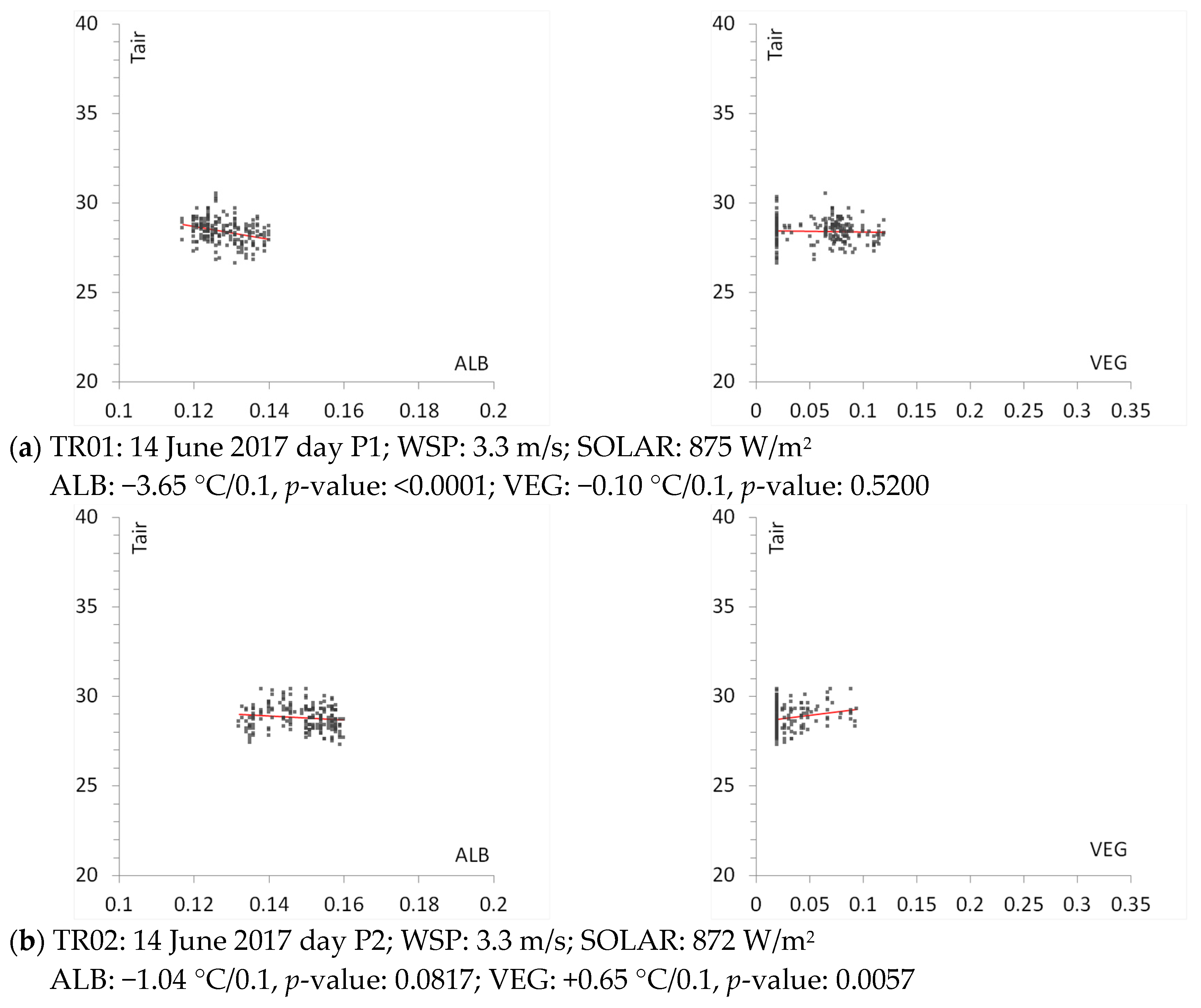
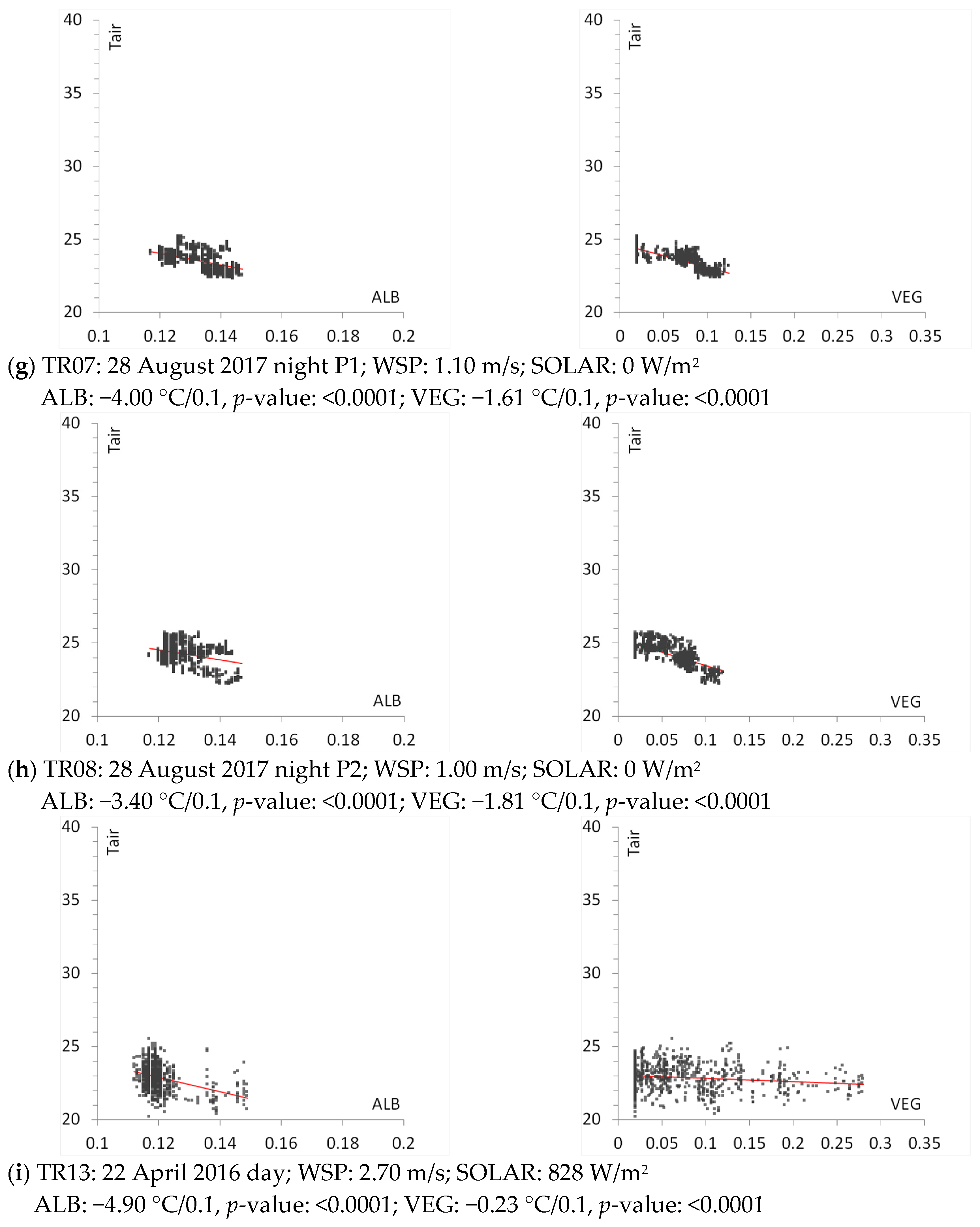
In 
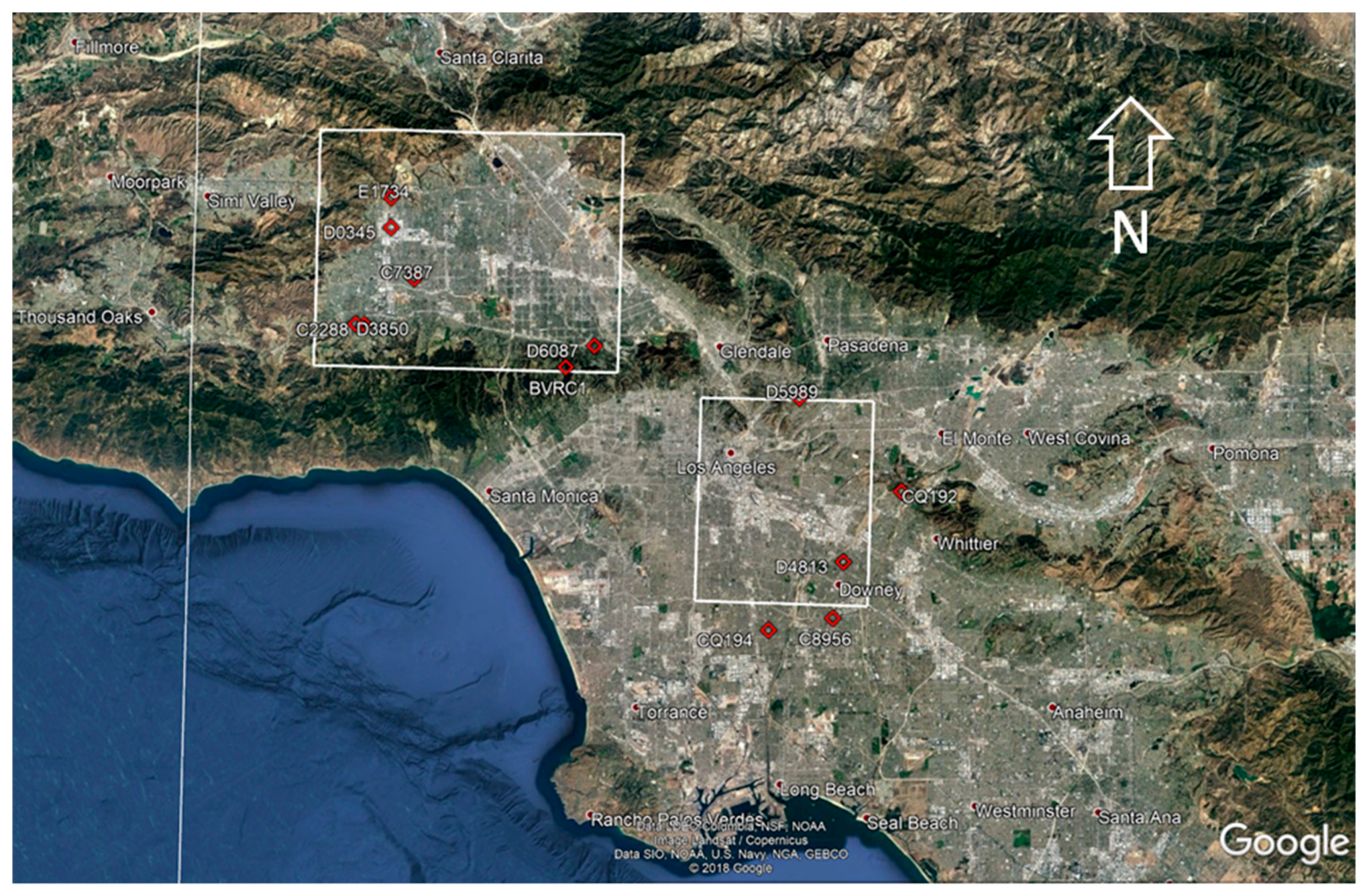
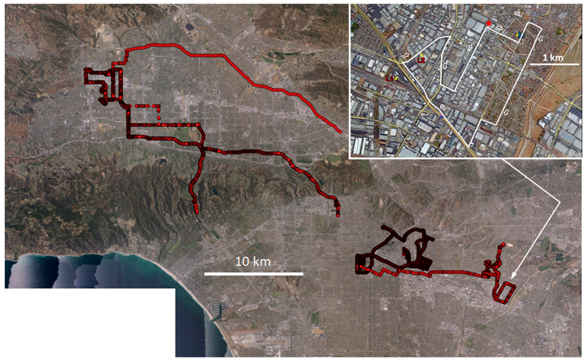
Figure 9a–i, observed air temperature (°C) from mobile transects is plotted on the vertical axis against grid-level (neighborhood-scale) albedo (ALB) or canopy cover (VEG), where ALB and VEG are each computed via Equations (1) and (2). This analysis is for the downtown area defined by the rectangle on the right in Figure 1. For the San Fernando Valley (domain defined by white rectangle on the left in Figure 1), the observed temperature in Figure 10a–e is plotted against canopy cover only (as predictor) because albedo has a smaller variability in this domain.
The analysis in Figure 9 and Figure 10 provides information for each transect segment including dates, slopes computed as temperature change per 0.1 increase in albedo or canopy cover (to normalize and facilitate inter-comparisons of effects across various transects), corresponding p-values (probability values), wind speed (WSP), and solar radiation (SOLRAD) at the time of the transect. The latter two were obtained from the NOAA/MADIS mesonet monitors closest to each mobile transect at the time it was conducted. In this analysis, a significance level of 0.05 was selected and, as such, a p-value < 0.05 represents a statistically significant correlation between observed temperature (from the transect) and surface properties (albedo and canopy cover).
The analysis in Figure 9 and Figure 10 was based on the Cressman-weighting scheme discussed above and a radius of influence of 1 km. The fifteen transects are identified as TR01 through TR15 and if a transect is made up of parts carried out at different times, these will be indicated as P1, P2, etc. One transect (TR14) is not shown in this analysis because of missing data.
Table 4 summarizes the main takeaways from the analysis in Figure 9 and Figure 10. It shows the response of observed air temperature (°C) to a 0.1 increase in neighborhood-scale albedo, symbolically written as ΔT/(0.1Δa), or in canopy cover, written as ΔT/(0.1Δη), in columns 2 and 6, along with the corresponding p-value for each transect (in columns 3 and 7, respectively). Again, the reason for selecting a denominator of 0.1 is simply to normalize the temperature sensitivity and facilitate inter-comparisons of the effects across various transects. Also, an increase of 0.1 in neighborhood-scale albedo and/or canopy cover is one assumption often made as a mitigation scenario in UHI studies. Hence, it is used here as an indicator to what the real-world impact might be on air temperature.
Except for two entries (contribution of canopy cover to air temperature in transect TR01 and contribution of albedo to air temperature in transect TR02, as seen in columns 7 and 3, respectively), all other entries are statistically significant. For these two transects, the p-values suggest that in TR01, albedo is the main driver of air temperature and in TR02, canopy cover is the main driver.
In addition, all correlations are negative (i.e., when albedo and/or canopy cover increase, temperature decreases) except for transects TR02 (for canopy cover, column 6) and TR03 (for albedo, column 2). As will be discussed next, these two transects were among those carried out during periods of higher wind speeds, which can weaken the correlations. In transects TR04 and TR05, the large temperature response (sensitivity) to albedo change is likely caused by the extensive freeway and roof cover in these areas (>95%).
Columns 4 and 8 show the actual range of albedo and canopy cover, respectively, associated with each specific transect instead of a hypothetical range of 0.1 as used in columns 2 and 6. In other words, the ranges of albedo and canopy cover in columns 4 and 8 are “bounded” by the values encountered in the real world at each of these transects.
Columns 5 and 9 are temperature changes (°C) computed by multiplying the corresponding actual range (from columns 4 or 8, respectively) by the slope given in columns 2 or 6 and dividing by 0.1. Thus the bounded temperature variations in columns 5 and 9 represent the maximum changes that can be expected in each specific transect (per its actual albedo or canopy-cover range) rather than the unbounded values in columns 2 and 6. By doing so, some of the unreasonably large slopes (unbounded) in column 2, e.g., for TR04 and TR05, become much more reasonable when bounded, as in column 5.
Thus, columns 5 and 9 represent the changes in temperature that one can expect as a result of increasing albedo and/or canopy cover by the amounts already encountered in the real world and that are achievable via current practices in building and planning. On the other hand, columns 2 and 6 represent the potential cooling effects that would result from implementations of high-albedo measures (cool roofs and cool pavements) and/or urban forestation, where each would be increased by 0.1.
Next, the correlations between mobile-observed temperature and albedo and/or canopy cover are re-examined but with a smaller radius of influence (<500 m). The goal is to evaluate whether a length-scale effect exists in these correlations. This analysis is done by comparing observations directly to surface properties at grid points, that is, without the Cressman analysis discussed above.
This analysis shows that the correlations between observed temperature and neighborhood-scale albedo and/or canopy cover are negative and statically significant at R < 500 m when wind speed is under 3 m/s locally—compare the p-values of rows 1, 3, 5, 7, and 9 in the right half of Table 5 with all the rows in the left half, suggesting weaker correlation between temperature and surface properties within 500 m at wind speeds exceeding 3 m/s. That is, when wind speed exceeds 3 m/s, the correlations either become weaker (for one of the predictors or the other) or statistically insignificant (see TR01, TR02, TR03, TR10, and TR15). For these cases, the analysis was repeated once more by (1) increasing the radius of influence from 500 m to 1 km and (2) restricting the correlations to upwind model points.
In this repeated analysis, the correlations improved further, i.e., some positive or weak correlations converted into negative or stronger ones as seen in Table 5 (compare TR01-SE to TR01, TR02-NW to TR02, TR03-NE to TR03, TR10-NW to TR10, and TR15-NE to TR10). In these cases, the p-values and slopes improved after increasing the upwind fetch (from 500 m to 1 km) and including only grid points within the wind approach direction. This also explains why these adjusted correlations are better than the corresponding ones in Table 4 (in some cases) for one or the other predictors, since the correlations in Table 4 were not limited to upwind points. For example, comparing TR01-SE from Table 5 to TR01 from Table 4, we can see that whereas the albedo-temperature correlation becomes a little weaker, the canopy-temperature correlation becomes much more significant (p-value changes from 0.53 to 0.0087). Comparing TR02-NW (Table 5) to TR02 (Table 4) shows a slight improvement in the significance of the albedo-temperature correlation and also a change in sign (from 0.65 to −0.11) for canopy-temperature correlation, albeit at a larger p-value. In this case, therefore, the temperature is driven by the albedo effect mainly. For TR03-NE there are mixed effects: whilst TR03-NE is improved relative to TR03 (in Table 5), it is not as good as the correlation for TR03 in Table 4 (this transect appears to be an exception). Finally, for TR10-NW and TR15-NW (in Table 5 relative to Table 4), the correlations do not change much.
Thus the results from this analysis suggest that when wind speed is less than 3 m/s, the observed temperature is influenced by the physical properties of the immediate surroundings (less than 500 m radius). At wind speeds exceeding 3 m/s, temperature is influenced by surface properties in a longer fetch (~1 km) in the upwind direction. Physically, this is because advective effects are smaller than the localized convective effects when wind speed is lower. At higher wind speed, in this case >3 m/s, temperature is influenced more by advective than localized effects. To provide context, the monthly average wind speeds in the study areas (from climatology) for January–December are 3.7, 3.5, 3.3, 3.1, 3.1, 2.6, 2.3, 2.2, 2.6, 2.6, 3.1, and 4.0 m/s, respectively. Thus the 3.3–4.0 m/s winds that were observed during some of the transects are relatively uncommon in this area and time of year, i.e., July and August, where 2.2–2.6 m/s is a more typical range. Of note, while there likely is a smooth transition around the 3-m/s threshold, we do not have observational values slightly under or over 3 m/s that can be used to evaluate this transition. Thus the suggested threshold of 3 m/s, while not a hard cutoff, is the most representative value that we determined based on the statistical analysis discussed above.

3.3.2. Multiple Regression

Multiple regression was carried out for albedo and canopy cover as predictors to observed air temperature from the transects. This analysis applies only to the downtown area since the San Fernando Valley analysis involved only variations in one predictor, canopy cover.
Here, the form of the correlation is given by Equation (3) where a is albedo and η is canopy cover. The coefficients (C1, C2, C3) and corresponding p-values (p1, p2, p3) are given in Table 6 and Table 7. Coefficients C1, C2, and C3 are in °C, and the “0.1” denominator simply indicates that the changes in temperature (C2 and C3) correspond to a 0.1 increase in surface albedo or a 0.1 increase in canopy cover. This was done for reasons explained in Section 3.3.1.
T air = C 1 + C 2 0.1     a + C 3 0.1     η
Following the structure of the discussion above, results from the multiple-regression analysis are presented in two parts; Table 6 summarizes the analysis at a 1-km radius of influence using the Cressman-type weighting discussed earlier, while Table 7 summarizes the 500-m analysis without weighting. The results in Table 6 show that the correlations are overwhelmingly negative (as albedo and canopy cover increase, temperature decreases) and statistically significant except for three situations. These are in transect TR01, where the role of the canopy cover is insignificant, and in transects TR02 and TR03, where the role of albedo is insignificant. This was already discussed in Section 3.3.1, as were the large slopes in TR04 and TR05.
In Table 7, and as introduced in Section 3.3.1, the sign of some correlations change to negative or significance improves (smaller p-values) when the radius of influence is increased and wind from a specific direction is accounted for rather than an average from several directions (e.g., TR01-SE and TR02-NW). In other words, at wind speeds exceeding 3 m/s, extending the upwind fetch from 500 m to 1 km and accounting for LULC properties only in the wind-approach direction improves the p-values and/or the coefficients for albedo and/or canopy cover changes. This is similar to what was found in Section 3.3.1.
The values listed in Table 6 and Table 7 are relative to changes of 0.1 in albedo or vegetation cover and, thus, are unbounded. These can be converted into transect-specific bounded values as was done in 
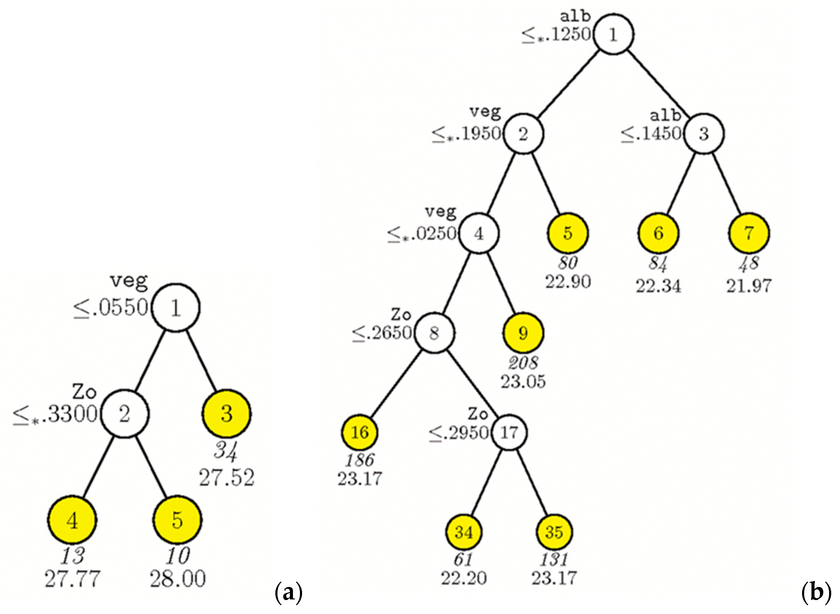
Table 4. Two examples are demonstrated here that will be referred to in the following discussion of example CART for transects TR04 and TR13 in Section 3.3.3. The first example is the coefficient C3 (for canopy cover) in Table 7, corresponding to transect TR04 with a value of −0.417 °C. If this is multiplied by the actual canopy-cover range of 0.1 (from Table 4, TR04 under column 8) and divided by 0.1, we obtain a bounded value of −0.41 °C. The second example is the coefficient C2 (for albedo) in Table 7, corresponding to transect TR13 (value of −2.088 °C). If this is multiplied by the actual albedo range of 0.037 (Table 4, transect TR13, under column 4), and divided by 0.1, we obtain a bounded value of −0.77 °C.

3.3.3. Classification and Regression Tree (CART)

A classification and regression tree (CART) analysis was also undertaken to assess the interactions among predictors of observed air temperature (from the mobile transects). The purpose of the CART analysis was to identify the main driver (albedo or canopy cover) of air temperature in each case, i.e., in various transect segments, because of variations in land use and surface physical properties. In addition, the roughness length parameter, computed following the approach of MacDonald et al. [30], was included in the following CART examples as an additional predictor to evaluate its role relative to that of albedo and canopy cover.
While the CART analysis was carried out for each of the 15 transects, two examples are presented here. Transect TR04 is a daytime transect at 14:00 Pacific Daylight saving Time (PDT) carried out on 14 June 2017 in the downtown area; TR13 also a daytime (13:00 PDT) transect in the downtown area, was carried out on 22 April 2016.
From the CART analysis of TR04 (Figure 11a), the following can be deduced:
  • In this transect segment, canopy cover (top node) is the main splitting variable, i.e., the main driver of air temperature. The lowest temperatures are associated with the highest canopy cover (node 3).
  • To estimate the influence of canopy cover on temperature in this sub-segment, we compare terminal nodes 3, 4, and 5. The difference between temperature at node 3 and the weighted temperatures at nodes 4 and 5 is −0.35 °C, which is the contribution of canopy-cover change to air temperature in this sub-segment. This is comparable to the value −0.41 °C computed above, in the last paragraph of Section 3.3.2 (based on the multiple regression in Table 7). The reduction in air temperature is significant, considering that this is a short segment (57 temperature observations).
  • Roughness length has minor, secondary effects. Within the range of lower canopy cover (<0.055), roughness length (Zo) can play a role. In this case, the larger Zo (node 5) produces slightly higher air temperatures (0.23 °C warmer on average) during daytime.
Transect TR13 is a longer segment with 798 temperature observations. The following can be deduced from this CART analysis (Figure 11b):
  • In this transect segment, the most influential variable on air temperature (top splitting node) is albedo.
  • Observed temperature is lower where albedo is larger. For neighborhood-scale albedo greater than 0.125, the temperatures are lowest, e.g., compare terminal nodes 6 and 7 (temperatures of 22.34 and 21.97 °C) with nodes 5, 9, 16, 34, and 35 (with higher temperatures of 22.90, 23.05, 23.17, 22.20, and 23.17 °C, respectively).
  • Calculating the weighted temperature differences for nodes with albedo higher then 0.125 (6 and 7) versus lower than 0.125 (nodes 5, 9, 16, 34, and 35) shows that the contribution of higher albedo in this transect is to lower air temperature by 0.81 °C, which is significant. This is comparable to the value of −0.77 °C computed in the last paragraph of Section 3.3.2, which was based on multiple regression.
  • Furthermore, within each subtree, the effects of increased albedo are evident. For example, comparing terminal nodes 6 and 7 shows that observed temperatures are 0.37 °C lower where albedo is larger than 0.145 relative to where albedo is lower than that.
  • In this transect, where albedo is lower than 0.125, canopy cover also has a significant effect. Comparing node 5 (where canopy cover is greater than 0.195) and nodes 9, 16, 34, and 35 (where cover is lower than 0.195), the contribution of canopy cover is to cool the air by 0.12 °C. This effect is smaller than the effects of albedo in this transect.
  • The effects of roughness length are secondary and different from one subtree to another. For instance, whereas increased roughness length in node 35 relative to node 34 does show increased temperature, comparing the increased roughness in nodes 34 and 35 relative to node 16, shows the opposite effect.

4. Conclusions

Fine-resolution meteorological modeling with a modified urbanized version of WRF was carried out as basis for siting fixed weather monitors and designing temperature mobile-observation routes. In combination, the modeling and observations were carried out to study urban heat in the Los Angeles region. A total of 15 observational mobile transects were carried out in the summers of 2016 and 2017. The mobile-observation temperatures were compared to model fields and also correlated to surface physical properties focusing on neighborhood-scale albedo and vegetation canopy cover.
Evaluation of coarse-scale regional simulations and fine-scale, transect-specific simulations against observations shows a meteorological-model performance that meets or is better than community-recommended benchmarks. For example, the temperature mean absolute error for transect-specific simulations is 0.86 °C (compare to a recommended threshold of ≤2 °C). The performance evaluation demonstrates that the model can be used in siting fixed weather stations and designing mobile-observation routes to characterize urban heat and cool islands.
The model results and observational data analysis (measurements from mobile transects) show that as albedo increases, air temperature decreases during the day, but also at night in smaller extents likely because of lag effects or masking by other variables (co-variance). The increase in canopy cover lowers air temperature during both day and night via combined effects of canopy shading, soil moisture, roughness, and evapotranspiration. The unbounded correlation between temperature and albedo or canopy cover, are both negative, ranging from −1.0 to −9.0 °C per 0.1 increase in neighborhood-scale albedo (or larger) and from −0.1 to −2.2 °C per 0.1 increase in canopy cover, except for a few cases with co-varying influences. While both albedo and canopy cover have significant impacts on air temperature, CART analysis done in this study also shows that, depending on land-use, surface physical properties, and geographical location, that one or the other becomes the main driver of air temperature.
At the 500-m scale, the analysis of observed temperature from mobile transects indicates that the negative correlations between air temperature and surface albedo and/or canopy cover become weaker or statistically insignificant at wind speeds exceeding about 3 m/s. For observations when wind speeds exceeded this threshold, the analysis was repeated to increase the radius of influence (from 500 m to 1 km) and to consider land use and surface physical properties in the upwind fetch only (wind approach direction). This resulted in the correlations becoming stronger (lower p-values and statistically more significant) and, where they were positive, the correlations became negative.
Of relevance to policy recommendations, the results from model, simple and multiple regressions, and CART analyses demonstrate the significant real-world cooling potential of increasing neighborhood-scale albedo and canopy cover. Based on bounded correlations between observed temperature and transect-specific ranges of albedo and canopy cover, the analysis shows that cooling of up to 2.8 °C during the daytime can be achieved by increasing neighborhood-scale (500-m) albedo. Cooling of up to 2.3 °C during the day and up to 3.3 °C at night can be achieved by increasing canopy cover. The changes in albedo and canopy cover that resulted in these amounts of cooling are actual neighborhood-scale variations already encountered in the real world in the Los Angeles area. This ability to cool a neighborhood will have added significance during excessive heat events or future climates when the warmer weather exacerbates urban heat.

Author Contributions

H.T., R.L., A.M., H.G, and G.B-W. conceived and designed the study; H.T. performed the land-use analysis, atmospheric modeling, analysis of simulation results, and statistical analysis of observations; R.L. and S.C. designed and built the air temperature measurement apparatus; A.M. and G.B-W. conducted the mobile transects; H.G. managed the project and coordination with partners; H.T. wrote the paper.

Acknowledgments

This work was funded by the California Energy Commission under Contract No. EPC-14-073. The effort from Lawrence Berkeley National Laboratory was also supported by the Assistant Secretary for Energy Efficiency and Renewable Energy, Office of Building Technology, State, and Community Programs, of the U.S. Department of Energy under Contract No. DE-AC02-05CH11231. We would like to acknowledge the support of the City of Los Angeles’ Department of Water and Power Bureau of Street Services; City of Los Angeles’ Mayor’s Office of Sustainability and Office of Resilience, County of Los Angeles, Los Angeles Unified School District, and California’s Department of Forestry and Fire Protection for providing data and informing selection of study areas. We also acknowledge the Southern California Association of Governments, the City of Los Angeles, and EarthDefine/CAL FIRE for providing high-resolution land-use and land-cover datasets. Tianbo Tang and Joseph Ko (University of Southern California) and Angie Rodriguez (National Autonomous University of Mexico) are acknowledged for assisting in carrying out mobile-transect observations and in the installation of fixed weather monitors.

Conflicts of Interest

The authors declare no conflicts of interest.

References

  1. Taha, H. Meteorological, emissions, and air-quality modeling of heat-island mitigation: Recent findings for California, USA. Int. J. Low Carbon Technol. 2013, 10, 3–14. [Google Scholar] [CrossRef]
  2. Sailor, D.; Shepherd, M.; Sheridan, S.; Tone, B.; Kalkstein, L.; Russell, A.; Vargo, J.; Andersen, T. Improving heat-related health outcomes in an urban environment with science-based policy. Sustainability 2016, 8, 1015. [Google Scholar] [CrossRef]
  3. Taha, H. Characterization of Urban Heat and Exacerbation: Development of a Heat Island Index for California. Climate 2017, 5, 59. [Google Scholar] [CrossRef]
  4. Vahmani, P.; Ban-Weiss, G.A. Impact of remotely sensed albedo and vegetation fraction on simulation of urban climate in WRF-urban canopy model: A case study of the urban heat island in Los Angeles. J. Geophys. Res. 2016, 121, 1511–1531. [Google Scholar] [CrossRef]
  5. Mavrakou, T.; Polydoros, A.; Cartalis, C.; Santamouris, M. Recognition of thermal hot and cold spots in urban areas in support of mitigation plans to counteract overheating: Application for Athens. Climate 2018, 6, 16. [Google Scholar] [CrossRef]
  6. Vahmani, P.; Sun, F.; Hall, A.; Ban-Weiss, G.A. Investigating the climate impacts of urbanization and the potential for cool roofs to counter future climate change in Los Angeles. Environ. Res. Lett. 2016, 11. [Google Scholar] [CrossRef]
  7. Taha, H. Meso-urban meteorological and photochemical modeling of heat island mitigation. Atmos. Environ. 2008, 42, 8795–8809. [Google Scholar] [CrossRef]
  8. Alexander, P.G.; Mills, G. Local climate classification and Dublin’s urban heat island. Atmosphere 2014, 5, 755–774. [Google Scholar] [CrossRef]
  9. Georgakis, C.; Santamouris, M. Determination of the surface and canopy urban heat island in Athens central zone using advanced monitoring. Climate 2017, 5, 97. [Google Scholar] [CrossRef]
  10. Mohegh, A.; Rosado, P.; Jin, L.; Millstein, D.; Levinson, R.; Ban-Weiss, G.A. Modeling the climate impacts of deploying solar reflective cool pavements in California cities. J. Geophys. Res. 2017. [Google Scholar] [CrossRef]
  11. Zhang, J.; Zhang, K.; Liu, J.; Ban-Weiss, G.A. Revisiting the climate impacts of cool roofs around the globe using an earth system model. Environ. Res. Lett. 2016, 11. [Google Scholar] [CrossRef]
  12. Taleghani, M.; Sailor, D.; Ban-Weiss, G.A. Micrometeorological simulations to predict the impacts of heat mitigation strategies on pedestrian thermal comfort in a Los Angeles neighborhood. Environ. Res. Lett. 2016, 11, 1–12. [Google Scholar] [CrossRef]
  13. Jin, H.; Cui, P.; Wong, N.H.; Ignatius, M. Assessing the effects of urban morphology parameters on microclimate in Singapore to control the urban heat island effect. Sustainability 2018, 10, 206. [Google Scholar] [CrossRef]
  14. Qiu, G.Y.; Zou, Z.; Li, X.; Li, H.; Guo, Q.; Yan, C.; Tan, S. Experimental studies on the effects of green space and evapotranspiration on urban heat island in a subtropical megacity in China. Habitat Int. 2017, 68, 30–42. [Google Scholar] [CrossRef]
  15. Tsin, P.K.; Knudby, A.; Krayenhoff, E.S.; Ho, H.C.; Brauer, M.; Henderson, S.B. Microscale mobile monitoring of urban air temperature. Urban Clim. 2016, 18, 58–72. [Google Scholar] [CrossRef]
  16. Jonsson, P. Vegetation as an urban climate control in the subtropical city of Gaborone, Botswana. Int. J. Climatol. 2004, 24, 1307–1322. [Google Scholar] [CrossRef] [Green Version]
  17. Sun, C.-Y.; Brazel, A.J.; Chow, W.T.L.; Hedquist, B.C.; Prashad, L. Desert heat sialnd study by mobile transect and remote sensing techniques. Theor. Appl. Climatol. 2009, 98, 323–335. [Google Scholar] [CrossRef]
  18. Ellis, K.N.; Hathaway, L.; Mason, R.; Howe, D.A.; Epps, T.H.; Brown, V.M. Summer temperature variability across four urban neighborhoods in Knoxville, Tennessee, USA. Theor. Appl. Climatol. 2017. [Google Scholar] [CrossRef]
  19. Taha, H. Cool cities: Counteracting potential climate change and its health impacts. In Current Climate Change Report; Invited Paper; Springer International Publishing: Cham Switzerland, 2015; Volume 1, pp. 163–175. [Google Scholar]
  20. Taha, H.; Freed, T. Creating and Mapping an Urban Heat Island Index for California. Report Prepared by Altostratus Inc. for the California Environmental Protection Agency (Cal/EPA); 2015. Available online: https://calepa.ca.gov/wp-content/uploads/sites/62/2016/10/UrbanHeat-Report-Report.pdf (accessed on 5 January 2018).
  21. Anderson, J.R.; Hardy, E.E.; Roach, J.T.; Witmer, R.E. A Land Use and Land Cover Classification System for Use with Remote Sensor Data; USGS Professional Paper 964; U.S. Government Printing Office: Washington, DC, USA, 2001.
  22. Ban-Weiss, G.A.; Woods, J.; Levinson, R. Using remote sensing to quantify albedo of roofs in seven California cities, Part 1: Methods. Sol. Energy 2015, 115, 777–790. [Google Scholar] [CrossRef] [Green Version]
  23. Multi-Resolution Land-Characteristics Consortium (MRLC), 2011. National Land Cover Databases. Available online: www.mrlc.gov (accessed on 15 June 2017).
  24. Ching, J.; Brown, M.; Burian, S.; Chen, F.; Cionco, R.; Hanna, A.; Hultgren, T.; McPherson, T.; Sailor, D.; Taha, H.; et al. National urban database and access portal tool, NUDAPT. Bull. Am. Meteorol. Soc. 2009. [Google Scholar] [CrossRef]
  25. Pleim, J.; Xiu, A.; Finkelstein, P.; Otte, T. A coupled land-surface and dry deposition model and comparison to field measurements of surface heat, moisture, and ozone fluxes. Water Air Soil Pollut. 2001, 1, 243–252. [Google Scholar] [CrossRef]
  26. Kusaka, H.; Kondo, H.; Kikegawa, Y.; Kimura, F. A simple single-layer urban canopy model for atmospheric models: Comparison with multi-layer and slab models. Bound.-Lay. Meteorol. 2001, 101, 329–358. [Google Scholar] [CrossRef]
  27. Tesche, T.W.; McNally, D.E.; Emery, C.A.; Tai, E. Evaluation of the MM5 Model over the Midwestern U.S. for Three 8-Hour Oxidant Episodes; Prepared for the Kansas City Ozone Technical Workgroup; Alpine Geophysics LLC: Arvada, CO, USA; Environ Corp.: San Rafael, CA, USA, 2001. [Google Scholar]
  28. Stewart, I.D.; Oke, T.R. Local climate zones for urban temperature studies. Bull. Am. Meteorol. Soc. 2012. [Google Scholar] [CrossRef]
  29. Millstein, D.; Levinson, R. Preparatory meteorological modeling and theoretical analysis for a neighborhood-scale cool roof demonstration. Urban Clim. 2018, 24, 616–632. [Google Scholar] [CrossRef]
  30. Macdonald, R.W.; Griffiths, R.F.; Hall, D.J. An improved method for estimation of surface roughness of obstacle arrays. Atmos. Environ. 1998, 32, 1857–1864. [Google Scholar] [CrossRef]
Figure 1. Urban WRF 500-m modeling domains for San Fernando Valley (left rectangle) and downtown area (right rectangle). Red diamonds locate the mesoscale network (mesonet) monitors closest to either domain. Downtown Los Angeles is near the northwest corner of the right rectangle.
Climate 06 00053 g001
Figure 2. Detail from the San Fernando Valley domain in Figure 1, showing 30-m tree cover (yellow: <10%, light green: 10–20%, black: >20% cover), building-specific roof albedo (red: 0.05–0.25, orange: 0.25–0.50, light orange: 0.50–0.90), and a sample mobile transect segment (white dots).
Climate 06 00053 g002
Figure 3. Mobile-transect apparatus.
Climate 06 00053 g003
Figure 4. Total DH for interval 1 in the downtown area 500-m domain. The unlabeled contours are only meant to show the spatial pattern of the temperature field.
Climate 06 00053 g004
Figure 5. Total DH for interval 1 in the San Fernando Valley 500-m domain. The unlabeled contours are only meant to show the spatial pattern of the temperature field.
Climate 06 00053 g005
Figure 6. Modeled total degree-hours (DH) for intervals 1–4 in the downtown area. The derived interval-average temperature (computed as DH/hour), blue to red, is as follows: 17.2–20.6 °C for interval 1; 21.3–25.3 °C for interval 2; 19.6–23.7 °C for interval 3; and 22.5–27.9 °C for interval 4.
Climate 06 00053 g006
Figure 7. Modeled total degree-hours (DH) for intervals 1–4 in the San Fernando Valley domain. The derived interval-average temperature (computed as DH/hour), blue to red, is as follows: 17.7–22.9 °C for interval 1; 22.0–27.5 °C for interval 2; 21.0–25.7 °C for interval 3; and 23.6–30.0 °C for interval 4.
Climate 06 00053 g007
Figure 8. Superimposed routes of 15 transects. Inset: a randomly-selected transect detail.
Climate 06 00053 g008
Figure 9. (ai): Observed air temperature (from mobile transects) versus neighborhood-scale albedo and canopy cover in the downtown area. Vertical axis (Tair) is air temperature (°C); horizontal axis is albedo (ALB) or canopy cover (VEG), unitless.
Climate 06 00053 g009aClimate 06 00053 g009bClimate 06 00053 g009c
Figure 10. (ae): Observed air temperature (from mobile transects) versus neighborhood-scale canopy cover in the San Fernando Valley domain. Vertical axis (Tair) is air temperature (°C); horizontal axis is canopy cover (VEG), unitless.
Climate 06 00053 g010aClimate 06 00053 g010b
Figure 11. CART for transects (a) TR04 and (b) TR13.
Climate 06 00053 g011
Table 1. Model performance indicators for seasonal simulations: bias, error, RMSE (root mean square error), and IOA (index of agreement). Model results were compared to observations from fixed monitor networks.
Performance IndicatorUnitsComputed Value
Wind speed bias m/s0.08
Wind speed RMSEm/s0.71
Wind speed IOA-0.80
Wind direction bias°0.92
Wind direction error°37.3
Temperature bias°C0.60
Temperature error°C2.10
Temperature IOA-0.95
Humidity biasg/kg−0.80
Humidity errorg/kg1.41
Humidity IOA-0.71
Table 2. Model performance metrics against observational mobile-transect temperature.
TransectMAE (°C)RMSE (°C)
2016_04_22 (west basin)1.151.33
2017_06_14 Part 1 (west basin)0.881.00
2017_06_14 Part 2 (west basin)0.610.76
2017_06_14 Part 3 (west basin)0.800.94
2017_06_14 Part 4 (west basin)0.700.86
2017_06_21 (San Fernando)1.732.00
2017_07_27 day Part 1 (San Fernando)0.971.20
2017_07_27 day Part 2 (San Fernando)0.921.10
2017_07_27 night Part 1 (San Fernando)0.550.68
2017_07_27 night Part 2 (San Fernando)0.851.00
2017_08_28 day Part 1 (west basin)0.480.60
2017_08_28 day Part 2 (west basin)0.710.94
2017_08_28 night Part 1 (west basin)1.001.10
2017_08_28 night Part 2 (west basin)0.820.92
Table 3. Comparison of model performance using standard and customized WRF-urban model.
Standard WRF-Urban Relative to Standard Non-Urban WRFModified WRF-Urban (Taha [3,7]) Relative to Standard Non-Urban WRF
Average over 2013, 2014, 2015Change in mean bias (°C)Change in mean error (°C)Change in mean bias (°C)Change in mean error (°C)
1–15 June −40%−4%−98%−28%
16–30 June −25%−6%−72%−31%
1–15 July −68%−4%−126%−15%
16–31 July −46%−7%−97%−26%
1–15 August −40%−7%−87%−26%
16–31 August −33%−6%−84%−25%
1–20 September −36%−5%−82%−25%
Table 4. Summary of observed transect temperature response to changes in neighborhood scale (500 m) albedo and/or canopy cover.
123456789
Albedo EffectsCanopy-Cover Effects
TransectΔT/(0.1Δa)p-valueActual Range (a)ΔT BoundedΔT/(0.1Δη)p-valueActual Range (η)ΔT Bounded
TR01−3.65<0.00010.023−0.84−0.100.53000.100−0.10
TR02−1.040.08170.021−0.220.650.00570.0540.35
TR031.000.00010.0170.17−0.400.00740.070−0.28
TR04−14.70<0.00010.012−1.76−0.890.00610.100−0.89
TR05−9.24<0.00010.030−2.77−2.20<0.00010.105−2.29
TR06−1.10<0.00010.038−0.38−0.40<0.00010.183−0.73
TR07−4.00<0.00010.030−1.20−1.61<0.00010.105−1.69
TR08−3.40<0.00010.030−1.02−1.81<0.00010.100−1.81
TR13−4.89<0.00010.037−1.81−0.22<0.00010.260−0.60
TR09 −0.40<0.00010.330−1.32
TR10−0.110.01050.304−0.33
TR11−0.20<0.00010.330−0.66
TR12−1.06<0.00010.313−3.31
TR15−0.53<0.00010.310−1.76
Table 5. Correlations between air temperature (°C) (observed from transects) and neighborhood-scale (500 m) albedo and/or canopy cover. Transects with wind direction represent effects from a 1-km upwind fetch.
TransectΔT/(0.1Δa)p-valueΔT/(0.1Δη)p-valuewind m/sTransectΔT/(0.1Δa)p-valueΔT/(0.1Δη)p-valuewind m/s
Wind speed < 3 m/sWind speed > 3 m/s
TR04−2.140.0120−0.530.00172.7TR01−0.830.05000.120.03703.3
TR05−5.03<0.0001−0.49<0.00011.3TR01-SE−0.950.0003−0.180.0087
TR06−1.08<0.0001−0.22<0.00012.2TR021.080.0007−0.220.10003.3
TR07−2.66<0.0001−0.41<0.00011.1TR02-NW−0.440.0414−0.110.6000
TR08−1.96<0.0001−0.50<0.00011.0TR031.410.0020−0.190.00033.4
TR13−2.35<0.0001−0.22<0.00012.7TR03-NE1.150.0010−0.300.0005
TR09 −0.18<0.00011.7TR10 0.080.00304.0
TR11−0.13<0.00011.3TR10-NW−0.070.0800
TR12−0.39<0.00010.0TR150.040.03303.3
TR15-NE−0.18<0.0001
Table 6. Equation (3) applied to a 1-km Cressman-type analysis of air temperature correlation to albedo and canopy cover. Coefficients C2 and C3 are, respectively, the responses of observed air temperature to a 0.1 increase in neighborhood-scale albedo and canopy cover.
TransectC1 (°C)p1C2 (°C)p2C3 (°C)p3
TR0133.25<0.0001−3.70<0.0001−0.150.3350
TR0231.65<0.0001−1.810.1204−1.080.0154
TR0329.42<0.0001−0.150.935−0.750.0086
TR0447.18<0.0001−13.95<0.0001−0.710.0052
TR0543.17<0.0001−8.17<0.0001−1.97<0.0001
TR0633.25<0.0001−0.78<0.0001−0.36<0.0001
TR0727.83<0.0001−2.42<0.0001−1.47<0.0001
TR0830.04<0.0001−3.71<0.0001−1.85<0.0001
TR1328.52<0.0001−4.63<0.0001−0.100.0500
Table 7. Equation (3) applied to a 500-m analysis of air temperature correlation to albedo and canopy cover without weighting (without and with correction for wind speed and direction). Coefficients C2 and C3 are, respectively, the responses of observed air temperature to a 0.1 increase in neighborhood-scale albedo and canopy cover.
TransectC1 (°C)p1C2 (°C)p2C3 (°C)p3
TR0129.28<0.0001−0.7650.050+0.1190.0266
TR01-SE29.59<0.0001−0.8810.010−0.0300.7000
TR0227.37<0.0001+1.0870.008−0.1480.2660
TR02-NW29.56<0.0001−0.4590.036−0.1610.5000
TR0329.94<0.0001−0.7020.100−0.2070.0005
TR0428.66<0.0001−0.4500.055−0.4170.1600
TR0537.41<0.0001−4.575<0.0001−0.238<0.0001
TR0633.98<0.0001−1.211<0.0001−0.353<0.0001
TR0725.93<0.0001−1.488<0.0001−0.334<0.0001
TR0827.21<0.0001−1.910<0.0001−0.491<0.0001
TR1325.49<0.0001−2.088<0.0001−0.120<0.0001

