1. Introduction
Atmosphere is highly variable over a large range of time and space scales. To understand environmental variability, continuous sampling measurements taken over time and space scales, which vary by many orders of magnitude, are essential. Environmental data can now be collected at time scales on the order of minutes, giving access to microscale information related to physical processes important for the urban built environment.
Many studies statistically analyze ambient air temperatures and the urban heat island phenomenon, and propose some data-driven modelling techniques, based mainly on hourly records [
1,
2,
3].
The high-frequency sampling is important to better understand small-scale couplings between different meteorological parameters (such as temperature, solar radiation, air velocity, and humidity) and buildings. In this framework, databases are being recorded so that multi-scale analyzing procedures can be applied, in order to be able to treat, exploit, and validate these datasets.
Even though the recording devices are often highly automated and give the means for online, real-time monitoring, they may possess a number of gaps, for many reasons. This being the case, many classical time series analysis methods, such as discrete-time Fourier transform, linear correlation analysis, multi-scale, or wavelet transform cannot be applied (see e.g., [
4,
5]).
Several authors have showed empirically that fluctuations of geophysical time series possess multifractal statistics.
Multifractals can be regarded as a rather considerable generalization of fractal geometry, developed for the description of geometrical patterns [
6] and the scaling relationship between patterns and the scale of measurement; the scale of a fractal set varies with the scale at which it is examined and raised to a scaling exponent, given by the fractal dimension. The extended multifractal fields concept [
7,
8,
9,
10,
11,
12,
13] can be considered as an infinite hierarchy of sets, each with its own fractal dimension. Thus, multifractals are described by scaling relationships that require a set of different exponents, rather than the single exponent of fractal patterns. Despite the apparent complexity of the multifractals, the distribution of a given scalar field can be wholly described by only three indices, using the universal multifractal formalism, as proposed by Schertzer and Lovejoy [
14,
15]. These indices resume the statistical behavior of turbulent fields from larger to smaller scales, as well as from extreme to mean behaviors.
The multifractal framework was largely developed for studying turbulent intermittency [
11,
16,
17,
18,
19,
20,
21]; it has been shown to be well-adapted for providing a parsimonious description of the statistics at all orders and over a wide range of scales for air temperature, air velocity, rainfall [
11,
22,
23], and for other intermittent geophysical fields [
24,
25,
26].
The aim of this paper is to further investigate the scaling behavior of air temperature data and its evolution with respect to the urban built environment. We therefore propose an approach to analyze high-frequency meteorological data, by adopting and applying time series analysis techniques in which missing data are well-respected: a frequency analysis through power spectral density estimation and a multi-scale structure functions analysis. To apply and assess the proposed approach, we use air temperature data recorded every 10 min by an autonomous monitoring system.
2. Materials and Methods
Here, we study high-frequency ambient air temperature data continuously monitored in Athens, Greece, during the period 2003. We use two different data sets provided from two different locations. The first data set, time series A, comes from a location suited in Athens University Campus, a sub-urban area on the outskirts of Ymitos Mountain. The second data set, time series B, comes from a monitoring system placed at the Western Athens Municipality, Peristeri, which is an urban area characterized by a high-density built environment and population. Temperature sensors where housed in a Stevenson screen 1.5 m above ground level.
Both time series consisted of data sampled every 10 min from 24 June 2003 to 21 August 2003. This corresponds to 8202 data points.
We performed spectral analysis, using extended discrete Fourier transform (EDFT), and multifractal analysis, using structure functions. Here follows a short description of the methods.
Spectral analysis corresponds to an analysis of variance, in which the total variance of a process is portioned into contributions arising from processes with different periodicities. Spectral analysis separates and measures the amount of variability occurring in different wave numbers of frequency bands. It characterizes the dynamics of the investigated series by associated scales and emphasizes periodicities, as well as forcing and scaling ranges. When all or part of the spectrum follows a power law, such as
where
f is the frequency, the data possess scaling statistics over this range. The velocity field for homogenous turbulence scales with a power spectrum slope of
[
27,
28]. The same slope is obtained for turbulent temperatures in homogeneous turbulence [
29,
30].
The fluctuation of time series that possess intermittent distributions can be studied using structure functions analysis, a simple yet powerful tool.
Assuming statistical time translational invariance, the structure function
, i.e., the statistical moments of the increment of the original series
, will depend only on the time lag
; in addition, according to a power law, if the process is scaling, then
where
T is the fixed, largest time scale of the system,
denotes the statistical average (for non-overlapping increments of length
),
q is the order of the moment (we take here
), and
is the scale-invariant structure function exponent. Structure function analysis corresponds, in fact, to studying “generalized” average volatilities at scale, since only moments of orders 1 or 2 are usually used to define the volatility. Furthermore, the present analysis consists in analyzing this generalized volatility for all time scales.
Intermittency can be characterized introducing scaling exponents from Equation (2). In this relation, since T is fixed, is a constant, and the main information is the time increment () dependence of the moments of fluctuations. The scaling exponent is estimated by the slope of the linear trends of versus in a log–log plot.
The average of the fluctuations corresponding to , i.e., the first moment, gives the scaling exponent , which is the so-called “Hurst” exponent characterizing the scaling non-conservation of the mean. The Hurst exponent provides a measure that characterizes the level of persistence in the time series. Values of H < 0.5 point to anti-persistency—i.e., a lower-than-average value tends to be followed by a higher-than-average value, and vice versa. A value of H = 0.5 signifies complete randomness, while values of H > 0.5 correspond to positive autocorrelation, and exhibit long memory that enables predictability.
The second moment is linked to the slope
β of the Fourier power spectrum [
16,
17,
18,
19,
20,
21,
22,
23,
24,
25,
26,
27,
28]:
The main property of a multifractal process is that it is characterized by a nonlinear
function [
16]. This function is convex, being proportional to the second Laplace characteristic function of the generator of cascade. Multifractals are the generic result of multiplicative cascades. A continuous-scale limit of such processes leads to the family of log-infinitely divisible distributions, among which are universal multifractals [
31], which have a normal or Levy generator, and for which
where
c1 is an intermittency parameter, and
is the basic parameter that characterizes the process. The index
c1 provides a measure that characterizes the mean inhomogeneity of the field: a value of
c1 = 0 corresponds to homogenous fields, while larger
c1 values correspond to more intermittent fields. The parameter
α is the Levy index, and indicates the extent of multifractality. It takes a value between 0 and 2, and can be understood as an interpolation between two extremes and well-known cascade models of turbulence: the β-model (
α = 0) and the lognormal model (
α = 2). The case 1 ≤
α ≤ 2 corresponds to a log–Levy process with unbounded singularities.
The above formulas indicate that universal multifractals can be characterized by only three parameters, in which α and c1 are the fundamental parameters, with α being the most basic.
For simple monofractal processes, is linear, e.g., for fractional Brownian motion (fBm) or for Brownian motion (Bm).
The deviation of the experimentally obtained curve from the linear trend is an indication of intermittent multifractal fluctuations, whose statistics are characterized by estimated for non-integer moment orders, up to moments of order 4 or 5, depending on the data sets.
The structure functions can be estimated even when there are missing values in the original time series. This can be expressed as:
where
is the number of consecutive data points
in the series, verifying
.
3. Results
Data set A possesses a percentage of missing values, due to Internet connection problems.
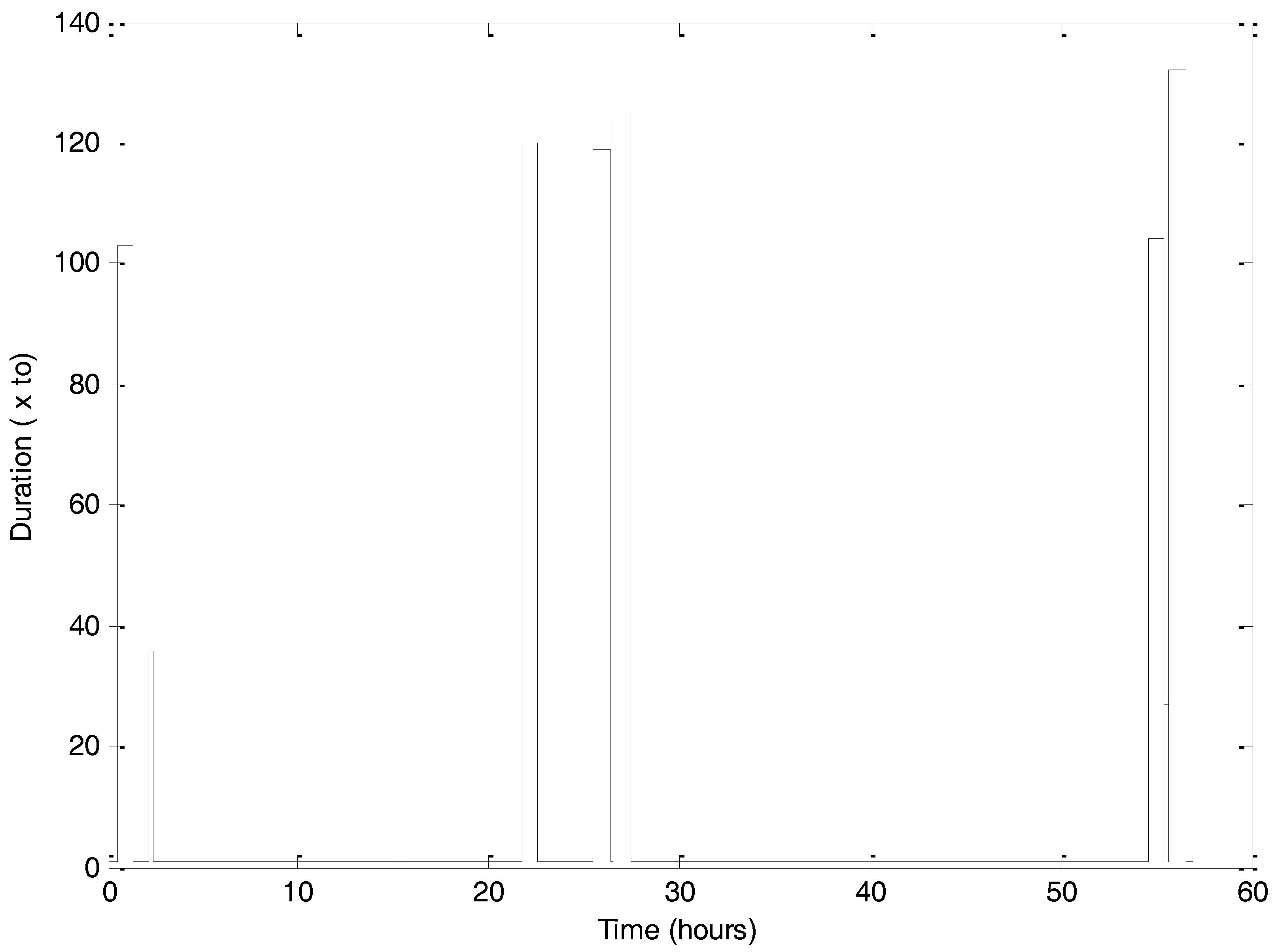
Figure 1 shows the multi-scale fluctuations of temperature for both data sets, as well as the succession of missing values in the time series for data set A. For time series B, there are no missing data. The time increments between successive values, normalized by the sampling time scale of
to = 10 min, present an inhomogeneous distribution, as shown in
Figure 2.
For time series A, the time interruption range was from 7to to 125to, with a mean value of 80.1to, which corresponds to 13.5 h mean interruption time.
3.1. Power Spectral Analysis of an Air Temperature Time Series
Power spectral analysis is often performed using a fast Fourier transform (FFT) algorithm. This algorithm cannot be directly applied to the data considered in the present work, because it requires continuously sampled data.
The problem of missing data is usually faced by averaging the data, or by filling in missing values with interpolated data. However, averaging corresponds to degraded resolution, while interpolation introduces additional artifacts. Another approach, adapted in the present work, is to directly analyze available data without losing scale information or introducing artificial correlations.
Thus, frequency spectra were obtained using extended discrete Fourier transform (EDFT), an algorithm for evaluating a Fourier transform even in the case of incomplete data and irregular sampling, as proposed by V. Liepins [
32].
Estimated frequency spectra for the two different temperature time series data are shown in
Figure 3, in a log–log plot. The frequency range is from 20 min to seven days.
In
Figure 2, vertical dotted lines correspond to specific time scales associated to periodic events or solar forcing: the diurnal periodicity and its harmonics (shown in the graph is the 8 h periodicity). For scales smaller than the 8 h solar forcing, the temperature power spectrum exhibits scaling behavior. Small scale fluctuations do not permit accurate estimation of the slope β. Nevertheless, a linear fit through the data gives approximate values of
b = 1.93 for time series A and
b = 1.87 for time series B. The slopes (straight lines) are plotted according to the estimate (see below) of the structure function scaling exponent, e.g.,
b = 2.7 for time series A and
b = 2.5 for time series B. The absence of characteristic time scales and the presence of a scaling range for scales smaller than 8 h lead us to perform multifractal analysis.
3.2. Multifractal Data Analysis
Here, we present the structure functions analysis of the two considered time series. In
Figure 4 and
Figure 5, we show the structure functions in log–log plot for different orders of moments. The scaling range previously revealed by the spectral analysis is confirmed. The straight lines show that the scaling of Equation (2) is very well-respected; scaling behavior is visible for scales between 10 min and 9 h for time series A, and between 10 min and 7 h for time series B; we repeated this for moments up to 6.0, with a 0.2 increment. The scaling begins to break only for moments up to 6.0, because of the insufficient amount of data analyzed.
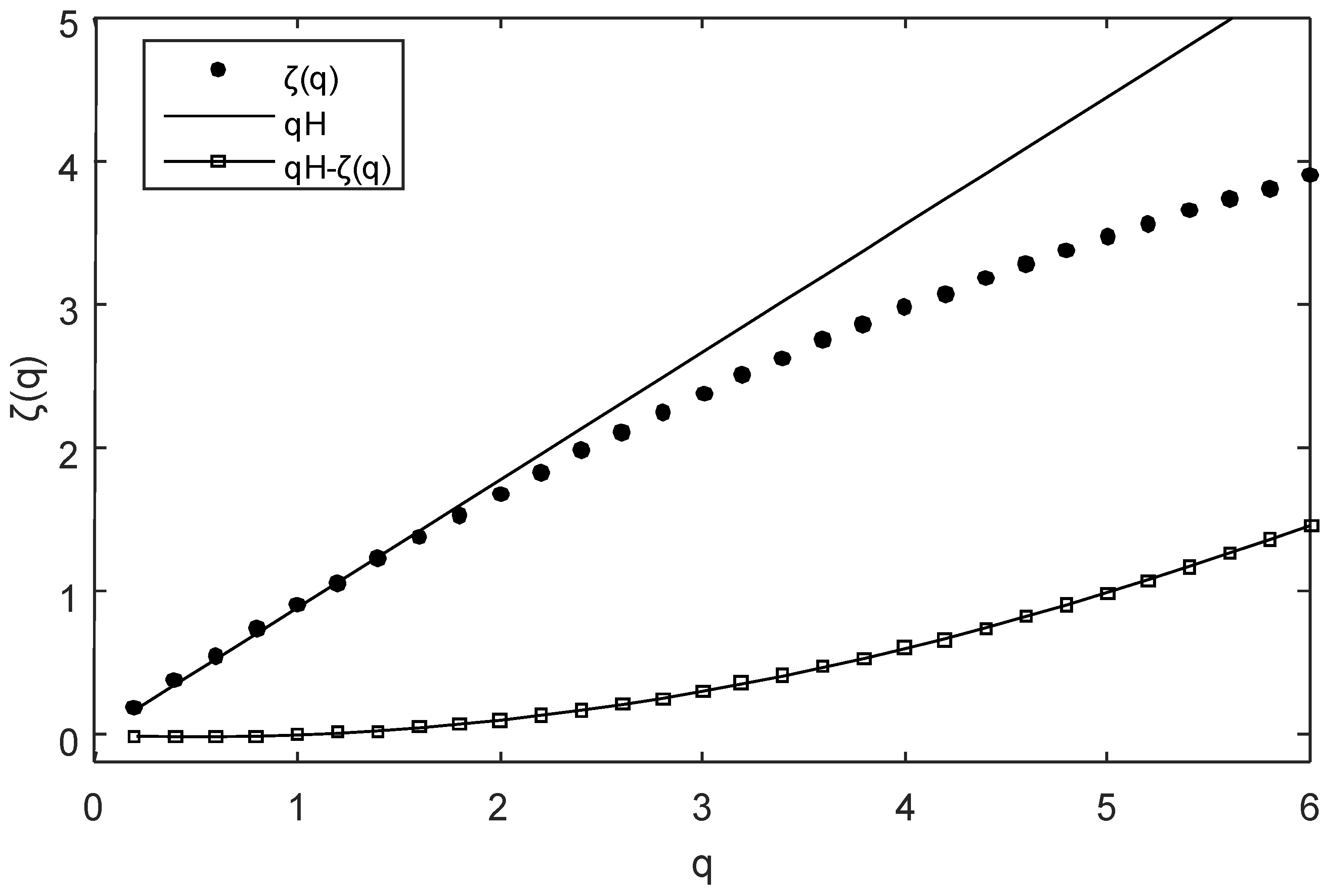
The resulting
functions are shown in
Figure 6 and
Figure 7; nonlinearity is present. We also directly estimated the scaling exponent of the nonlinear term
, which is a convex function plotted on the same graph.
We obtained the following values for the two time series: Η = 0.89 ± 0.01 for time series A and H = 0.74 ± 0.01 for time series B. Using specific analysis techniques, we obtained c1 = 0.0520 ± 0.0004 and α = 1.936 ± 0.008 for time series A, and c1 = 0.082 ± 0.002 and α = 1.79 ± 0.02 for time series B. We also obtained ζ(2) = 1.68 and ζ(2) = 1.35.
This indicates that in general, air temperature data are characterized by multifractal processes; the values of H are relative high, indicating also that the fluctuations are less variable than fluctuations found in homogenous turbulence.
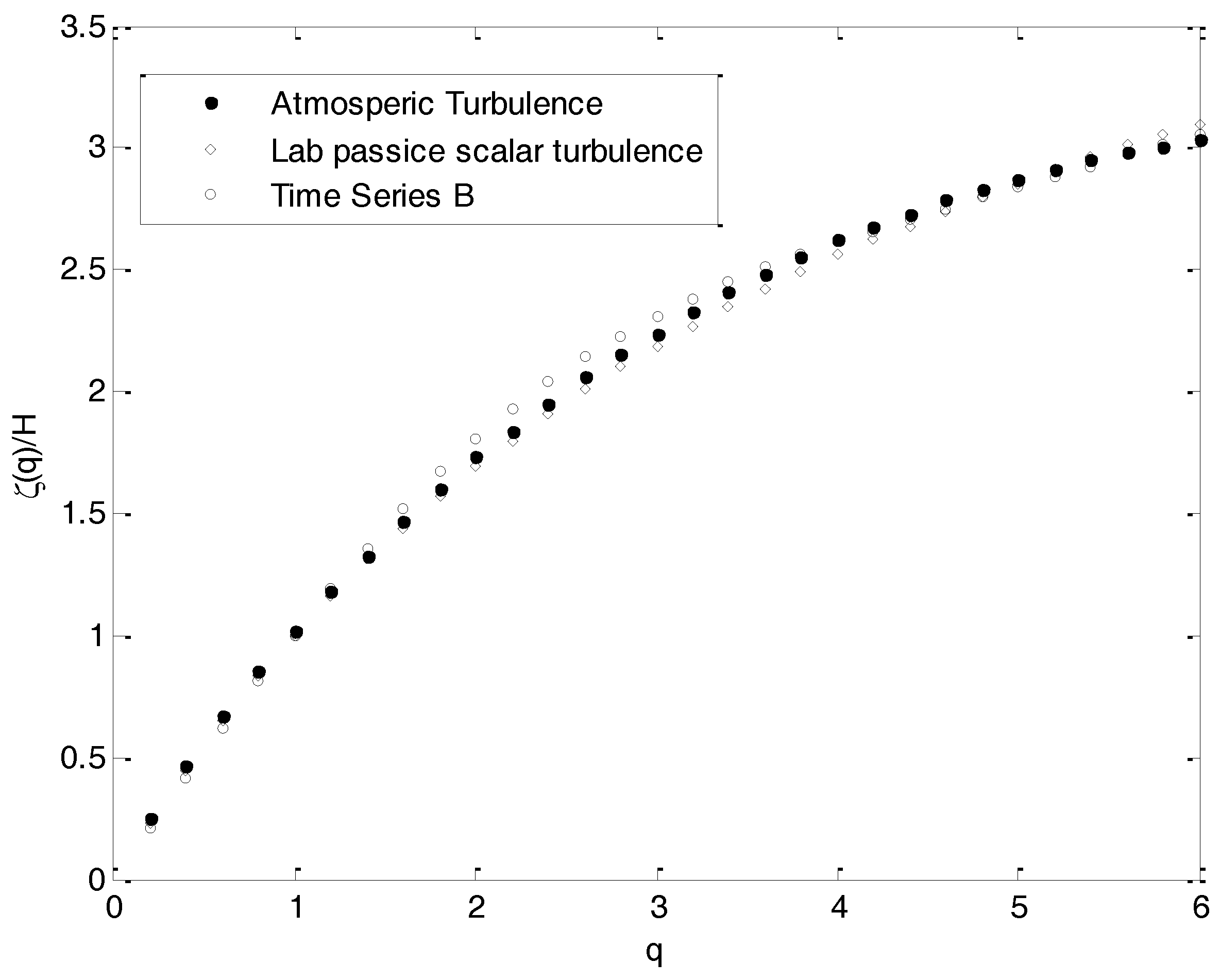
In
Figure 8, the normalized structure function scaling exponent
is also shown for turbulent atmospheric temperature data (
H = 0.38,
α = 1.45,
c1 = 0.34, [
21]) and for laboratory passive scalar turbulence (
H = 0.37, γ+ = 0.31,
c1 = 0.84, [
33]). The strong correspondence observed in this figure indicates that the universal models with the above parameters are compatible with the data through the medium range of moments, and probably reflect a general property of temperature fluctuations, which could be valid for small-scale turbulence and for temperature fluctuations at larger scales.
Figure 9 shows the
H spectra as a function of the temporal scale of ambient temperature for the two data sets. The scale range in the plots is from 1 h to around 10 h. For both data sets, a trend of decreasing
H values after around 4 h is evident. The suburban location’s air temperature plot show larger
H values, compared to
H values for urban location, for scales up to 4 h. For both data sets, this indicates increased persistence and good predictability up to these time scales. After this scale,
H decreased smoothly and reached the
H = 0.5 value, which implies random behavior and lack of predictability, at a time scale of about 9 h.
4. Discussion
In the years of information and communication technology expansion, time series will be continuously longer, providing a challenge to better understand and predict urban climate complex processes. Finding optimal ways to analyze these complex and possible nonlinear environmental time series data sets is therefore very important.
To explore these methods, we have analysed here ambient air temperature time series, sampled every 10 min throughout 2003 by an online environmental monitoring system for suburban and highly-built urban environments, in Athens, Greece. Missing data are well-respected in the sense that we neither average the data nor fill the gaps with interpolations; thus, any information concerning system’s dynamics is well-preserved.
Spectral analysis reveals a diffuse forcing around 12 h, while for smaller scales (from 10 min to 6–7 h), a turbulent-like behaviour has been observed. Multifractal structure functions analysis was applied, and provided the experimental estimate of scaling exponents ζ(q). We computed these scaling exponents for several values of q between 0 and 6; the clearly nonlinear bevariour of ζ(q) is direct evidence of the multifractal nature of air temperature.
We then studied and quantified this multifractality using the universal multifractal model. Using two different data sets, we obtained values of the three indices (H, c1, α) which can completely characterize the statistics of air temperature time series data. The low c1 values, 0.052 and 0.082 respectively for the air temperatures recorded at the suburban and the urban locations, indicate a homogenous field. Similarly, the high α values, 1.93 and 1.79, respectively, indicate that multifractality approaches its upper limit. Thus, both data sets present characteristics that are typical of log–Levy processes.
The differences between the calculated H, c1 and α parameters, although small, are greater than the statistical error. This indicate that urban locations, compared to suburban, are characterized by an increased heterogeneity, and that there are more large deviations from the mean; the high values of the air temperature do not dominate as much as for suburban locations. However, more data are needed for further analysis.
We compared the normalized structure function scaling exponents with turbulent atmospheric temperature data and laboratory passive scalar turbulence (see
Figure 8). The normalized values of the data are good, indicating that some of the general properties of temperature fluctuations valid for small-scale turbulence are preserved at larger scales.
Multifractal analysis can also be used to characterize the self-affinity of time series, through the detailed information about the Hurst parameter H. The Hurst parameter represents a temporal fractality measure, and thus can be used as a tool for assessing the time scale dependence of the predictability of air temperature. For the distinct range of time scales considered in the study, i.e., from 1 h up to around 9 h, air temperature behaves in a predictable way. Beyond this scale, H values become smaller than 0.5, indicating a decreasing predictability, probably due to the lack of local correlations. As far as it concerns quantitative predictability, our results indicate that statistical methods that are usually used to predict time series, like multiple linear regression (MLR), adaptive neuro-fuzzy inference systems (ANFIS), and neural networks (ANNs) can potentially be effective up to a prediction horizon of 10 h.
It appears that air temperature in urban and suburban environments is a complex time series, caused by the local correlations and interactions of various factors, such as topography, the built environment, and the atmosphere. More generally, the non-linearity of the empirical curve ζ(q) shows that the time series studied here can be considered as multifractals. Empirical curves are slightly different for the two time series, as the time series corresponding to the high-density built environment appear to be more convex. The differences between the calculated H, c1 and α parameters may indicate increasing heterogeneity and decreasing multifractality from suburban to urban locations.
Online monitoring systems and Information and Communication Technology (ICT) provide the framework to obtain databases that can facilitate data availability, as well as investigation of new methods and techniques. The time series analysis methods presented here may be generally applied to other environmental parameters as well, thus providing a way to improve our knowledge about the dynamics of environmental processes at the urban scale. Our results pertain to a certain geographical location, though we estimate that they can be confirmed and generalized by further studies, using data from other sites and climate zones.


