A New Radiative Model Derived from Solar Insolation, Albedo, and Bulk Atmospheric Emissivity: Application to Earth and Other Planets

Abstract
:1. Introduction
2. Materials and Methods
3. Results
3.1. Statement of the Model
3.2. Derivations of the Equilibrium and Non-Equilibrium Radiative Models
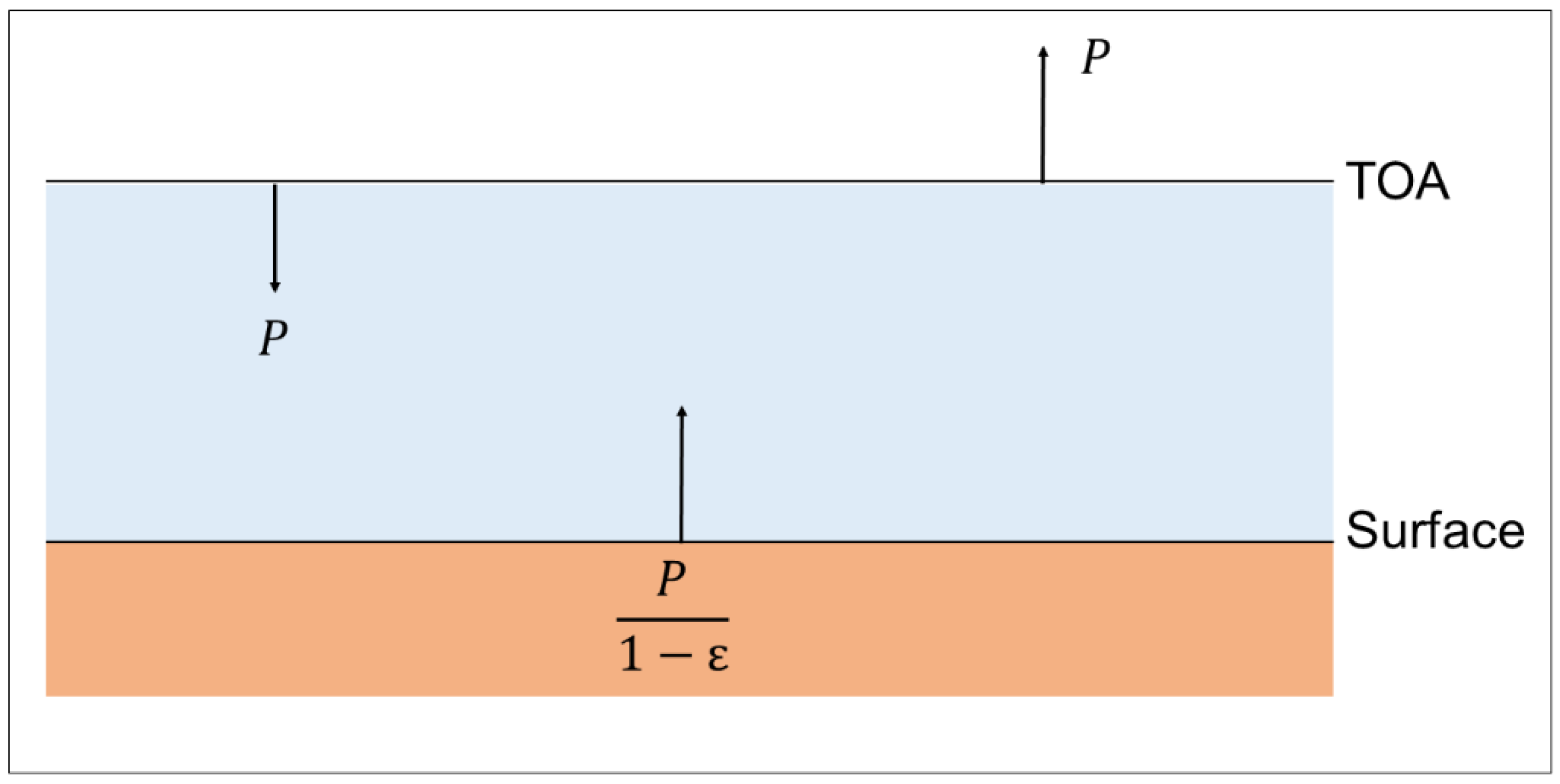
3.2.1. Properties of an Adiabatic Atmosphere
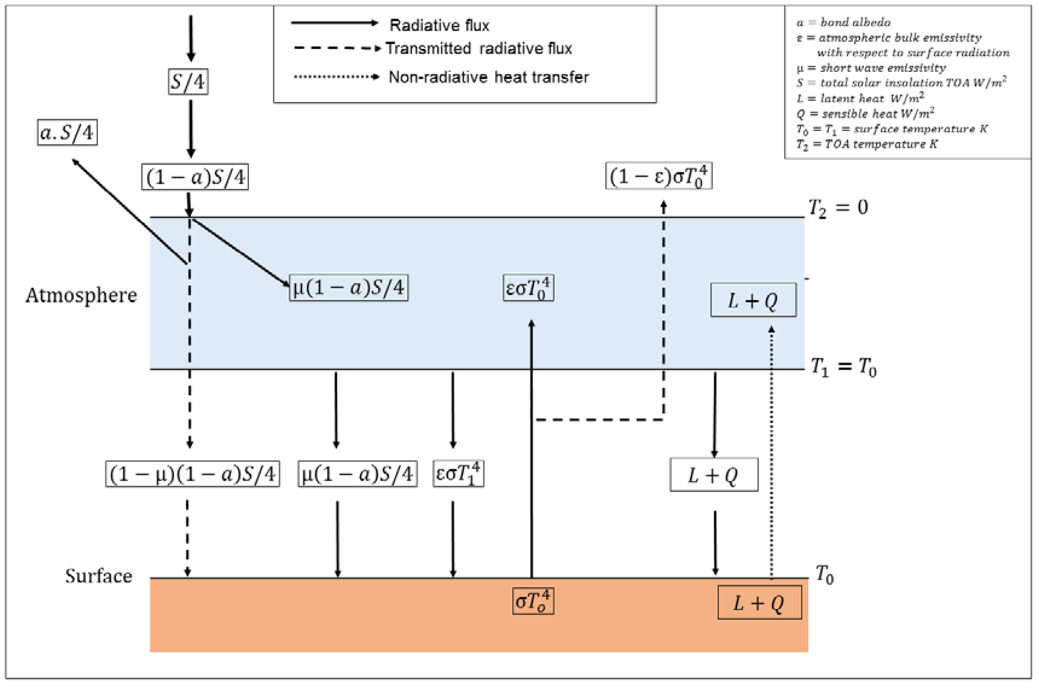
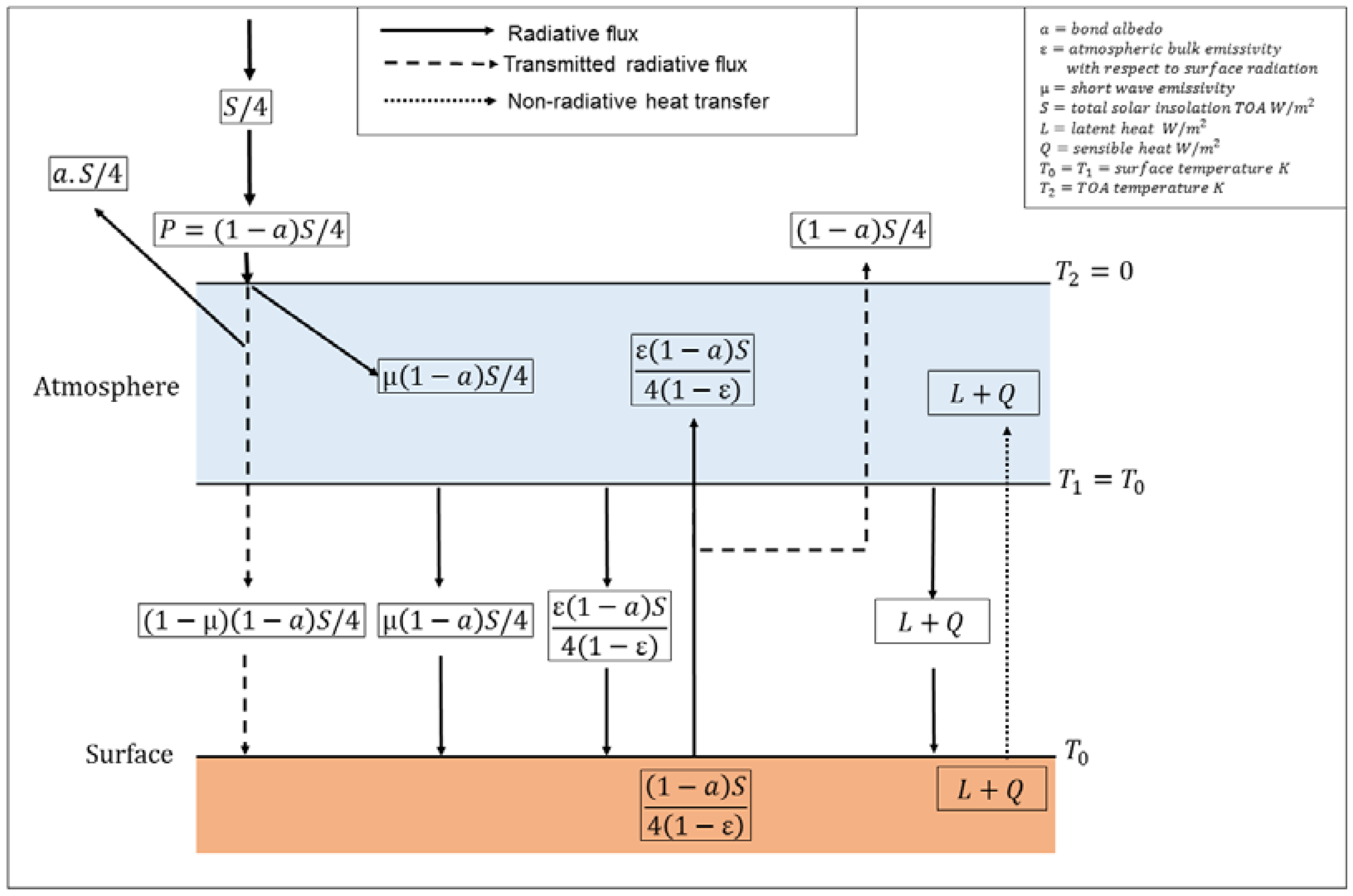
3.2.2. Derivation of the Equilibrium Adiabatic Radiative Model
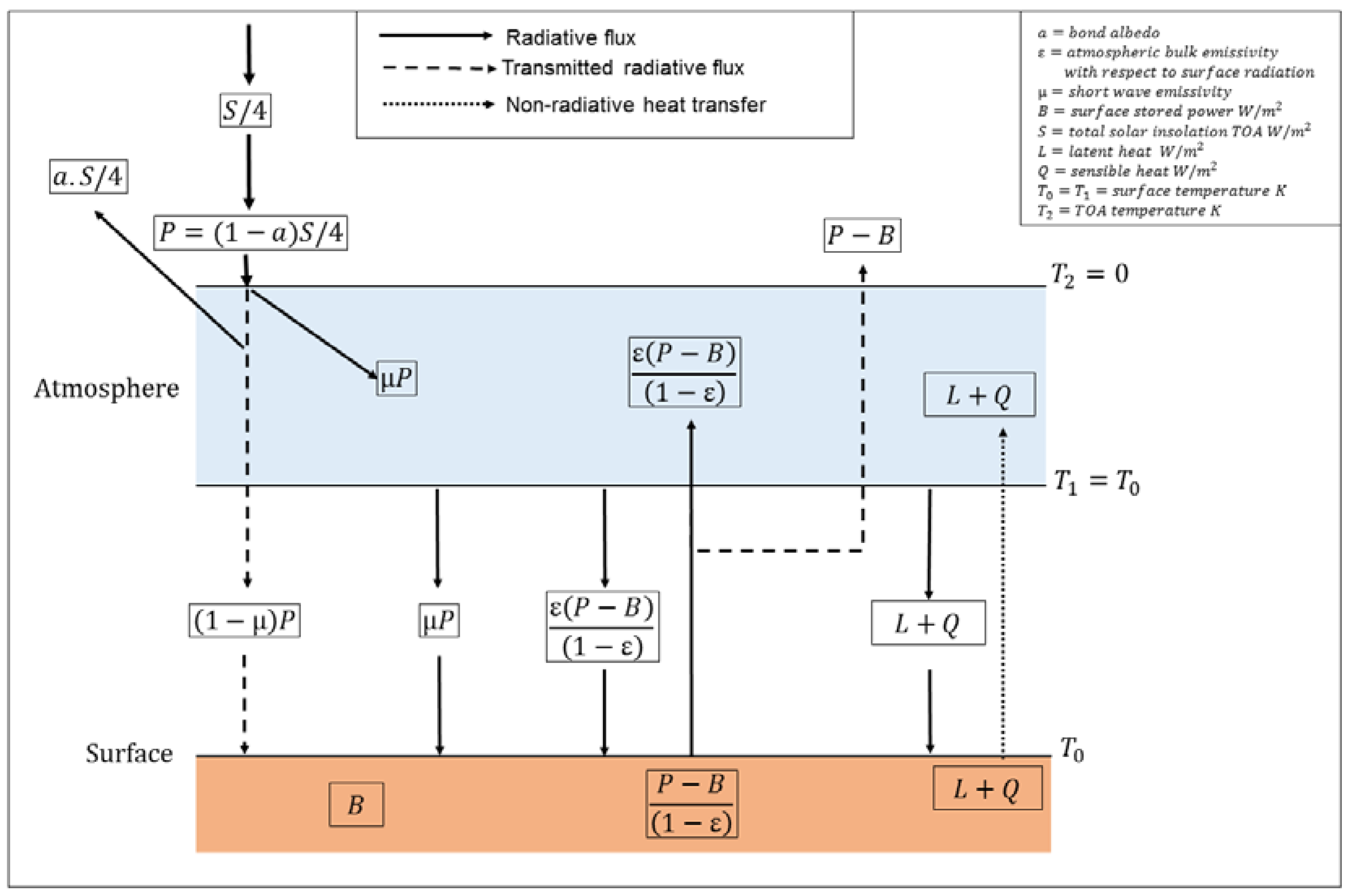
3.2.3. Derivation of the Non-Equilibrium Adiabatic Radiative Model
3.3. Validation of the Model by Comparison with Observations
3.4. Application of the Equilibrium Adiabatic Radiative Model to Planetary Bodies
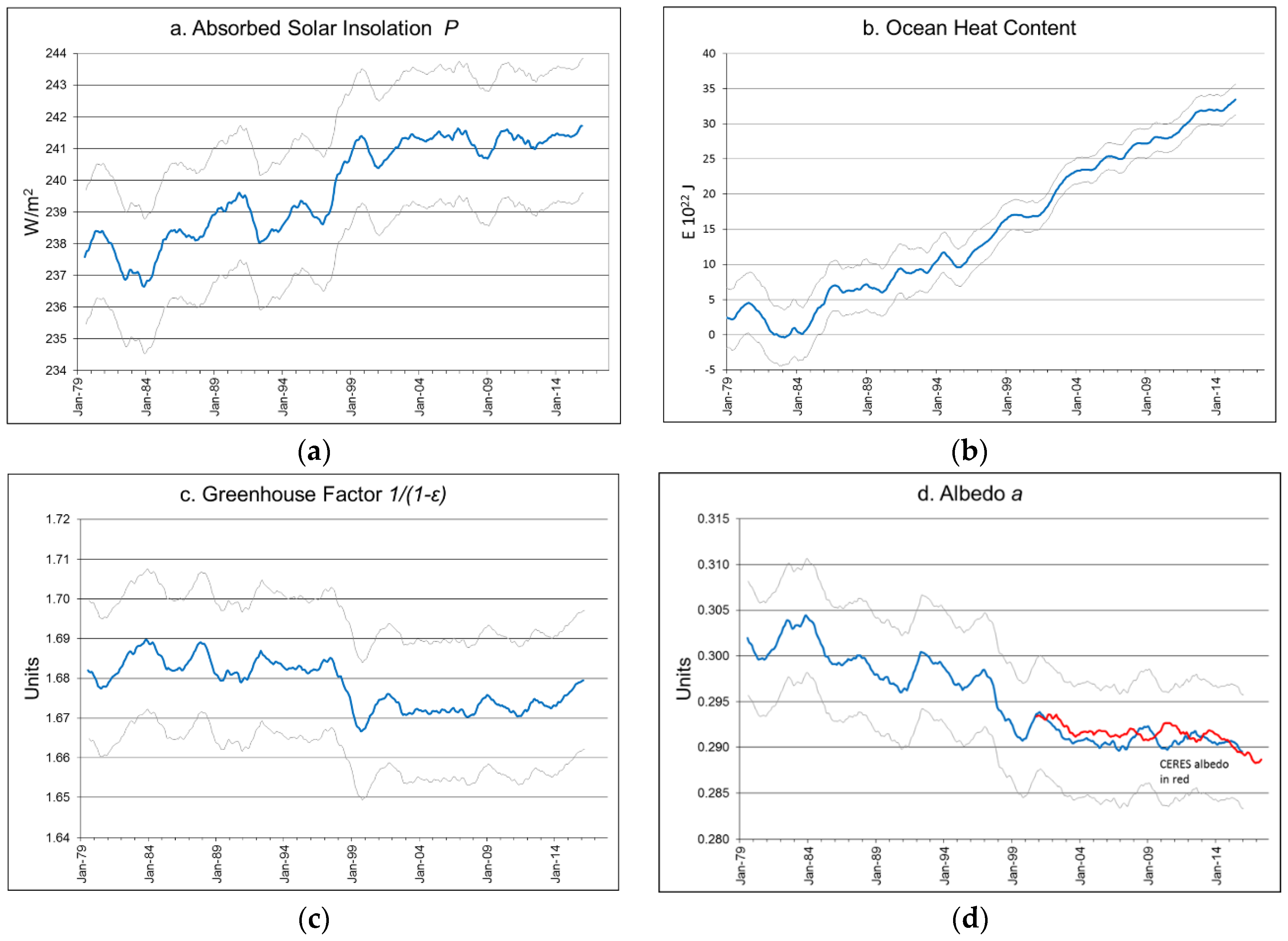
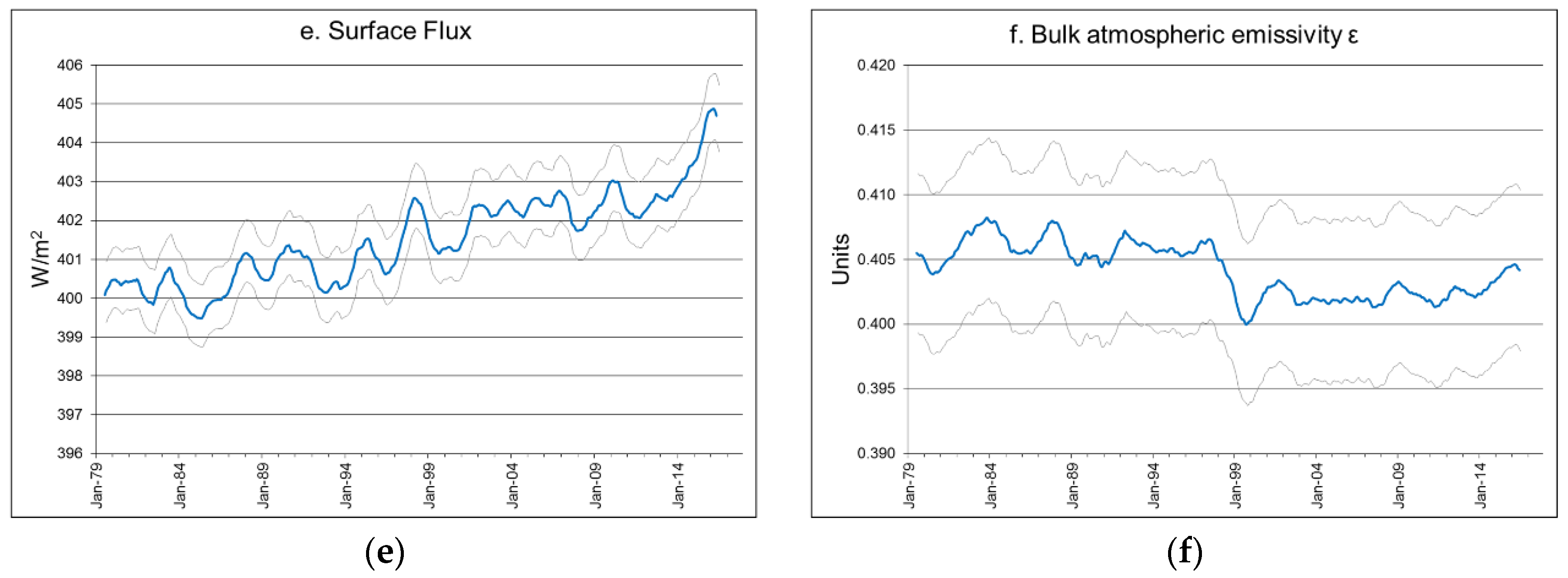
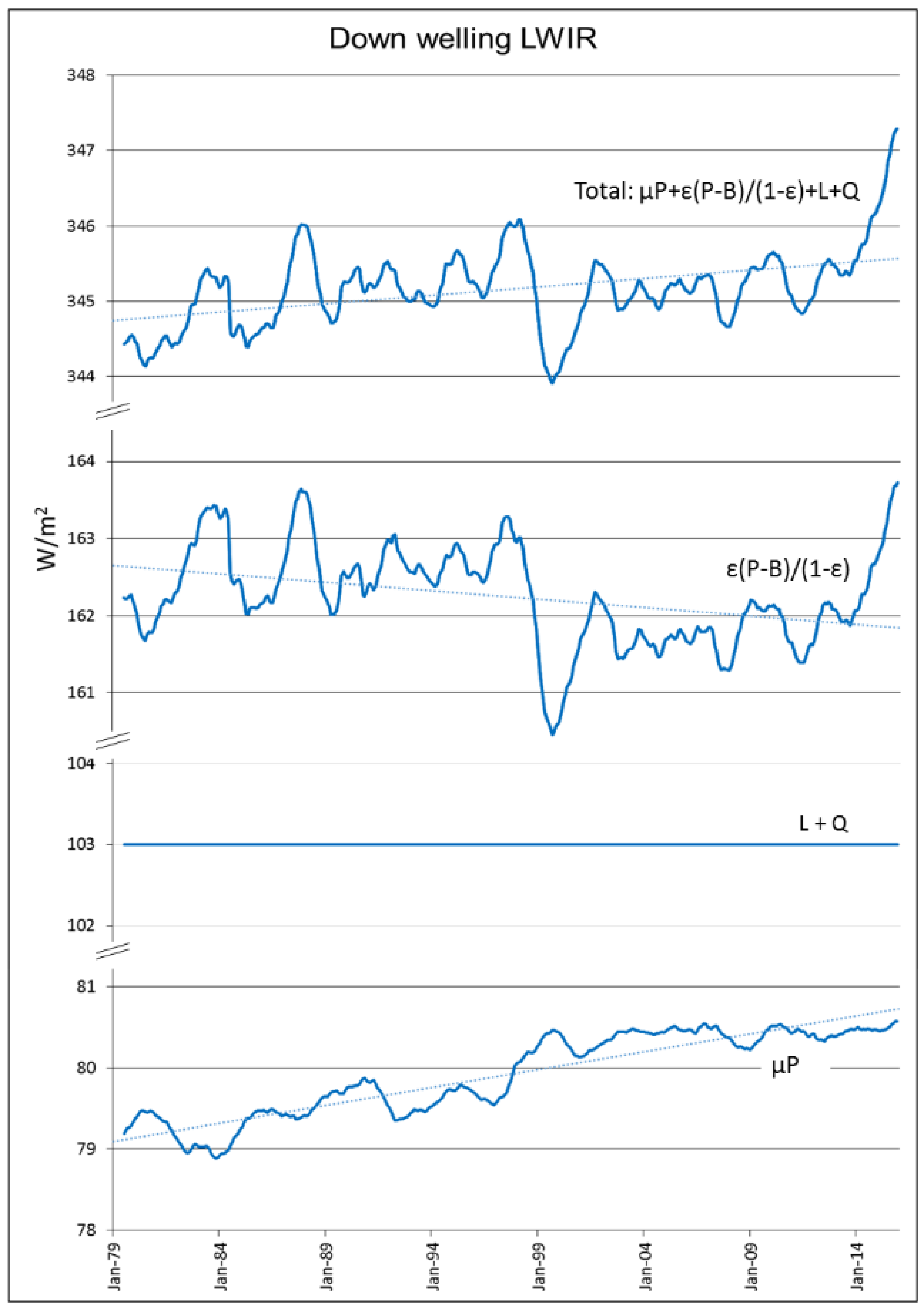
3.5. Application of the Non-Equilibrium Adiabatic Radiative Model to Earth
4. Discussion
Acknowledgments
Conflicts of Interest
References
- Rossow, W.B.; Zhang, Y.-C. Calculation of surface and top of atmosphere radiative fluxes from physical quantities based on ISCCP data sets. 2. Validation and first results. J. Geophys. Res. Atmos. 1995, 100, 1167–1197. [Google Scholar] [CrossRef]
- Kiehl, J.T.; Trenberth, K.E. Earth’s annual global mean energy budget. Bull. Am. Meteorol. Soc. 1997, 78, 197–208. [Google Scholar] [CrossRef]
- Wild, M.; Folini, D.; Schär, C.; Loeb, N.; Ellsworth, G.D.; König-Langlo, G. The global energy balance from a surface perspective. Clim. Dyn. 2013, 40, 3107–3134. [Google Scholar] [CrossRef]
- Wild, M.; Folini, D.; Hakuba, M.Z.; Schär, C.; Seneviratne, S.I.; Kato, S.; Rutan, D.; Ammann, C.; Wood, E.F.; König-Langlo, G. The energy balance over land and oceans: An assessment based on direct observations and CMIP5 climate models. Clim. Dyn. 2015, 44, 3393–3429. [Google Scholar] [CrossRef]
- Wild, M.; Ohmura, A.; Schar, C.; Muller, G.; Folini, D.; Schwarz, M.; Hakuba, M.Z.; Sanchez-Lorenzo, A. The Global Energy Balance Archive (GEBA) version 2017: A database for worldwide measured surface energy fluxes. Earth Syst. Sci. Data 2017, 9, 601–613. [Google Scholar] [CrossRef]
- Lee, H.T.; NOAA CDR Program. NOAA Climate Data Record (CDR) of Daily Outgoing Longwave Radiation (OLR); Version 1.2; NOAA National Climatic Data Center: Asheville, NC, USA, 2011. [CrossRef]
- Fröhlich, C. Observations of irradiance variations. Space Sci. Rev. 2000, 94, 15–24. [Google Scholar] [CrossRef]
- Huang, B.; Thorne, P.W.; Banzon, V.F.; Boyer, T.; Chepurin, G.; Lawrimore, J.H.; Menne, M.J.; Smith, T.M.; Vose, R.S.; Zhang, H.-M. NOAA Extended Reconstructed Sea Surface Temperature (ERSST); Version 5; NOAA National Centers for Environmental Information: Asheville, NC, USA, 2017.
- Fan, Y.; van den Dool, H. A global monthly land surface air temperature analysis for 1948–present. J. Geophys. Res. 2008, 113, D01103. [Google Scholar] [CrossRef]
- KNMI Climate Explorer. Available online: https://climexp.knmi.nl/start.cgi?id=someone@somewhere (accessed on 10 December 2017).
- Rossow, W.B.; Schiffer, R.A. Advances in understanding clouds from ISCCP. Bull. Am. Meteorol. Soc. 1999, 80, 2261–2288. [Google Scholar] [CrossRef]
- NVAP Science Team. NVAP-M Data; Atmospheric Science Data Center (ASDC): Hampton, VA, USA, 2013. Available online: https://eosweb.larc.nasa.gov/project/nvap/climate_total-precipitable-water_table (accessed on 10 December 2017).
- Vonder Haar, T.H.; Bytheway, J.L.; Forsythe, J.M. Weather and climate analyses using improved global water vapor observations. Geophys. Res. Lett. 2012, 39, L16802. [Google Scholar] [CrossRef]
- Cheng, L.; Trenberth, K.; Fasullo, T.; Boyer, T.; Abraham, J.; Zhu, J. Improved estimates of ocean heat content from 1960 to 2015. Sci. Adv. 2017, 3, e1601545. [Google Scholar] [CrossRef] [PubMed]
- Yelle, R.V.; Strobel, D.F.; Lellouch, E.; Gautier, D. Engineering Models for Titan’s Atmosphere. In Huygens: Science, Payload and Mission, Proceedings of an ESA Conference, Noordwijk, The Netherlands, 22–25 April 1997; Wilson, A., Ed.; ESA: Paris, France, 1997; pp. 243–256. [Google Scholar]
- Wielicki, B.A.; Barkstrom, B.R.; Harrison, E.F.; Lee, R.B.; Smith, G.L.; Cooper, J.E. Clouds and the earth’s radiant energy system (CERES): An earth observing system experiment. Bull. Am. Meteorol. Soc. 1996, 77, 853–868. [Google Scholar] [CrossRef]
- Gerlich, G.; Tscheuschner, R.D. On the Barometric Formulas and Their Derivation from Hydrodynamics and Thermodynamics. 2010. Available online: http://arxiv.org/pdf/1003.1508 (accessed on 10 December 2017).
- Hansen, J.; Nazarenko, L.; Ruedy, R.; Sato, M.; Willis, J.; Del Genio, A.; Koch, D.; Lacis, A.; Lo, K.; Menon, S.; et al. Earth’s energy imbalance: Confirmation and implications. Science 2005, 308. [Google Scholar] [CrossRef] [PubMed]
- NASA Planetary Fact Sheets. Available online: https://nssdc.gsfc.nasa.gov/planetary/planetfact.html (accessed on 10 December 2017).
- Lee, H.T.; Gruber, A. Development of the HIRS Outgoing Longwave Radiation Climate Dataset. Am. Meteorol. Soc. 2007. [Google Scholar] [CrossRef]
- Morice, C.P.; Kennedy, J.J.; Rayner, N.A.; Jones, P.D. Quantifying uncertainties in global and regional temperature change using an ensemble of observational estimates: The HadCRUT4 dataset. J. Geophys. Res. 2012, 117, D08101. [Google Scholar] [CrossRef]
- Palle, E.; Goode, P.R.; Montañés-Rodríguez, P.; Shumko, A.; Gonzalez-Merino, B.; Lombilla, C.M.; Jimenez-Ibarra, F.; Shumko, S.; Sanroma, E.; Hulist, A.; et al. Earth’s albedo variations 1998–2014 as measured from ground-based earthshine observations. Geophys. Res. Lett. 2016, 43, 4531–4538. [Google Scholar] [CrossRef]
- Trenberth, K.E.; Fasullo, J.T.; Kiehl, J. Earth’s Global Energy Budget. Bull. Am. Meteor. Soc. 2009, 90, 311–324. [Google Scholar] [CrossRef]


| Unit | Wild et al. Model | Adiabatic Radiative Model | ||
|---|---|---|---|---|
| Best Estimate | Uncertainty Range | Value | Calculated | |
| Variables | ||||
| S W/m2 | 1360 | 1360 | ||
| μ | 0.3333 | 0.3333 | ||
| ε | 0.3995 | 0.3995 | ||
| a | 0.2941 | 0.2941 | ||
| P = (1 − a)S/4 W/m2 | 240 | (1 − a)S/4 | 240 | |
| Fluxes, W/m2 | ||||
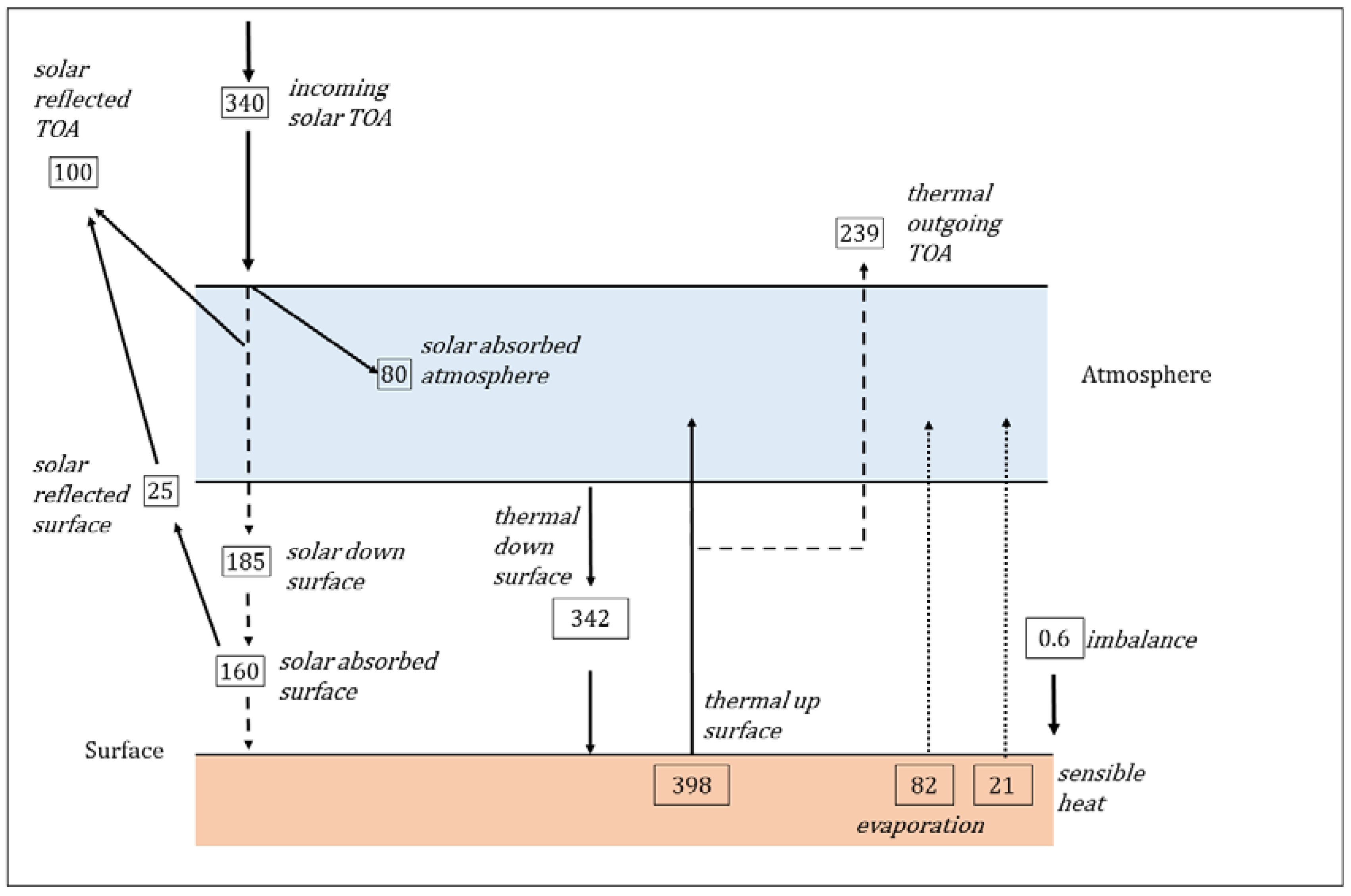
| Incoming solar TOA | 340 | 340–341 | S/4 | 340 |
| Solar absorbed by atmosphere | 80 | 74–91 | μP | 80 |
| Solar reflected TOA | 100 | 96–100 | a.S/4 | 100 |
| Solar down surface | 185 | 179–189 | not used | |
| Solar absorbed surface | 160 | 154–166 | (1 − μ)P | 160 |
| Solar reflected surface | 25 | 22–26 | not used | |
| Evaporation | 82 | 70–85 | - | - |
| Sensible heat | 21 | 15–25 | - | - |
| Evaporation + sensible heat | 103 | 85–110 | 103 1 | - |
| Thermal up surface | 398 | 394–400 | (P − B)/(1 − ε) | 398.6 |
| Thermal outgoing TOA | 239 | 236–242 | P − B | 239.4 |
| Thermal down surface | 342 | 338–348 | ε(P − B)/(1 − ε) + μP + L+ Q | 342.3 |
| Imbalance | 0.6 | 0.2–1 | B = 0.6 1 | |
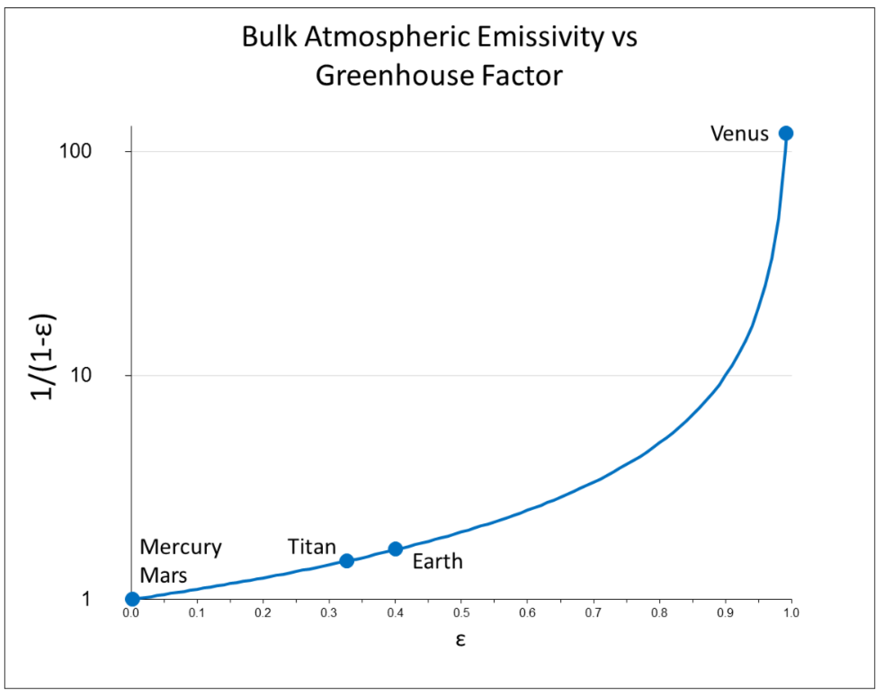
| PARAMETER | Mercury | Venus | Earth 1 | Mars | Titan |
|---|---|---|---|---|---|
| Average surface temperature K | 440 | 737 | 290 | 210 | 93 |
| Total solar flux S W/m2 | 9083 | 2601 | 1361 | 586 | 14.82 |
| Absorbed solar radiation P W/m2 | 2125 | 149 | 237 | 109.9 | 2.89 |
| Albedo | 0.07 | 0.77 | 0.3 | 0.250 | 0.22 |
| Atmospheric bulk emissivity ε | 0 | 0.991 | 0.407 | 0.0038 | 0.327 |
| Average surface flux W/m2 | 2125 | 16,728 | 400 | 110.3 | 4.30 |
| Greenhouse factor | 1 | 112 | 1.69 | 1.004 | 1.49 |
| Variables | CMIP5 | Adiabatic Model | Difference |
|---|---|---|---|
| S W/m2 | 1364.8 | ||
| μ | 0.310 | ||
| ε | 0.401 | ||
| a | 0.300 | ||
| B W/m2 | 1.00 | ||
| P = (1 − a)S/4 W/m2 | 238.9 | ||
| TOA components | Mean W/m2 | W/m2 | W/m2 |
| Solar down | 341.2 | 341.2 | 0 |
| Solar up | 102.3 | 102.3 | 0 |
| Solar net | 238.9 | 238.9 | 0 |
| Thermal up | 237.9 | 237.9 | 0 |
| Atmospheric components | |||
| Solar net | 74 | 74 | 0 |
| Thermal net | 179.2 | 178.8 | −0.4 |
| Surface components | |||
| Solar down | 189.4 | not used | |
| Solar up | 24.8 | not used | |
| Solar net | 164.8 | 164.9 | 0.1 |
| Thermal down | 338.2 | 337.8 | −0.4 |
| Thermal up | 396.9 | 396.9 | 0 |
| Thermal net | −58.7 | −59.1 | −0.4 |
| Net radiation | 106.2 | 105.8 | −0.4 |
| Latent heat | 85.4 | L = 85.4 | |
| Sensible heat | 19.4 | Q = 19.4 | |
© 2018 by the author. Licensee MDPI, Basel, Switzerland. This article is an open access article distributed under the terms and conditions of the Creative Commons Attribution (CC BY) license (http://creativecommons.org/licenses/by/4.0/).
Share and Cite
Swift, L. A New Radiative Model Derived from Solar Insolation, Albedo, and Bulk Atmospheric Emissivity: Application to Earth and Other Planets. Climate 2018, 6, 52. https://doi.org/10.3390/cli6020052
Swift L. A New Radiative Model Derived from Solar Insolation, Albedo, and Bulk Atmospheric Emissivity: Application to Earth and Other Planets. Climate. 2018; 6(2):52. https://doi.org/10.3390/cli6020052
Chicago/Turabian StyleSwift, Luke. 2018. "A New Radiative Model Derived from Solar Insolation, Albedo, and Bulk Atmospheric Emissivity: Application to Earth and Other Planets" Climate 6, no. 2: 52. https://doi.org/10.3390/cli6020052
APA StyleSwift, L. (2018). A New Radiative Model Derived from Solar Insolation, Albedo, and Bulk Atmospheric Emissivity: Application to Earth and Other Planets. Climate, 6(2), 52. https://doi.org/10.3390/cli6020052