1. Introduction
Decadal Climate Variability (DCV) involves persistent ocean-related phenomena existing on at least interdecadal timescales [
1,
2,
3,
4,
5]. Three forms of DCV are prominent: the Pacific Decadal Oscillation (PDO) [
6,
7,
8,
9,
10], the Tropical Atlantic Sea Surface Temperature Gradient (TAG) [
1], and the Western Pacific Warm Pool Sea Surface Temperature (WPWP) [
2,
11,
12]. Their main findings have been that the major ocean long-run temperature patterns have been associated with multiyear to multidecadal droughts in addition to changes in precipitation patterns.
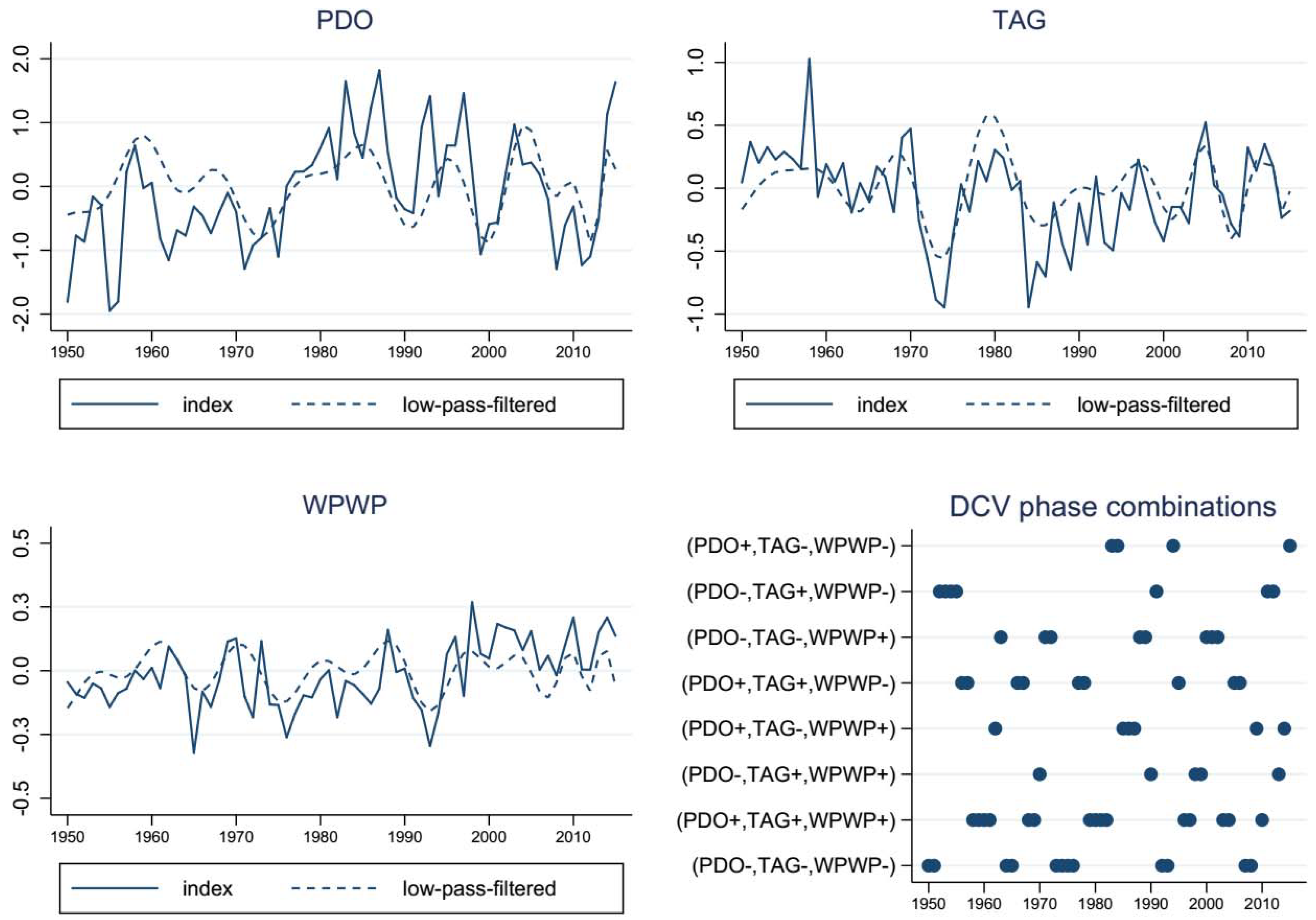
The PDO is a Pacific Ocean phenomenon that is characterized by two phases: warm and cold. Their phases are identified based on sea surface temperature (SST) anomalies in the North Pacific Ocean [
5,
13]. The PDO phase combinations have persisted for two or three decades in the 20th century [
9]. The PDO influences weather through mechanisms of heat transfer between the Pacific Ocean and the overlying atmosphere. Consequently, this phenomenon influences winds in the lower troposphere, and is associated with periods of prolonged dryness and wetness in the western United States and the Missouri River Basin [
3]. There is evidence of PDO impacts in the Southern Hemisphere, over the mid-latitude South Pacific Ocean, Australia, and South America [
9].
The TAG is a decadal El Niño-like pattern of Atlantic water characteristics that persists for 12 or 13 years. It also has two phase combinations, positive and negative. The TAG is identified through Atlantic sea surface temperature variations in the cross-equatorial dipole pattern [
1]. The TAG has been found to be associated with variability in many ocean and atmospheric forces, such as heat transferred between the overlying atmosphere and the Atlantic Ocean, winds in the lower troposphere, and rainfall in the southern, central, and midwestern United States [
3].
The WPWP is a western Pacific phenomenon and is associated with changes in ocean temperature and in turn with anomalies in surface area, land area temperature, and precipitation, which changes on a 10–15 year period. It is a region of sea surface temperatures warmer than 28.5 °C, extending from the eastern North Pacific to the Gulf of Mexico and the Caribbean on the west of Central America. At its peak, it expands to the tropical waters of tropical North Atlantic on the east [
11]. The WPWP exerts influence on the weather over the Great Plains with the positive phase combination and is associated with precipitation and temperature variation in the Great Plains and Western Corn Belt [
2].
Each DCV phenomenon has two phase combinations. Jointly, these DCV phenomena have been found to impact drought and extreme weather events over longer time frames [
4,
14]. Researchers have found that DCV-associated variations in major ocean long-run temperature patterns have been associated with multiyear to multidecadal droughts and changes in precipitation patterns [
2,
3,
4,
5,
13,
14,
15,
16,
17,
18].
Wang and Ting (2000) [
19] found a strong but geographically differentiated association between precipitation variability in the southeastern and northwestern United States and Pacific SST anomalies. Ting and Wang (1997) [
6] noted that the year-to-year fluctuations in summertime precipitation over the US Great Plains were significantly correlated with tropical and North Pacific SST variations. Wang et al. (2010) [
20] described increases in southeast summer precipitation variability as being primarily associated with SST warming in the Atlantic and also with SST variability across the equatorial Atlantic.
Méndez and Magaña (2010) [
21] found that SST anomalies in the North Pacific Ocean led to positive anomalies in the standardized precipitation index over the northeastern United States. They suggest that these anomalies weakened the intensity of the 1950s drought over this region. The Pacific SST was found to alter North American precipitation data [
16]. In particular, they found increases in Pacific SST were associated with increased precipitation in northern North America and the Mississippi basin and reduced precipitation over the southwest and eastern United States [
16].
Across these studies, the evidence shows the large-scale interdecadal variability of climate forces from North Atlantic Oscillation (NAO), PDO, and WPWP influences the precipitation variability on the Great Plains and the Midwest in addition to effects from El Niño–Southern Oscillation (ENSO) -precipitation variability [
22]. Mehta et al. (2012) [
18] found that the DCV phenomena have significant impacts in the Missouri River Basin (MRB), altering levels of precipitation and temperature variability plus the incidence of droughts and floods. Their findings indicate that the DCV phenomena explain 60–70% of the total variance in MRB annual precipitation and water supply. They also found that DCV has a large influence on maximum and minimum temperatures.
To the extent of the author’s knowledge from literature review, there are no studies on how the DCV phenomena can alter weather in the crop-growing seasons across the United States. This decadal climate variability study endeavors to advance the literature by reporting the empirical evidence of the impacts of these decadal climate phenomena on local hydroclimatic variables such as growing degree day, precipitation, and drought in the growing seasons of major economic crops, such as corn, soybeans, and wheat. The author conducts an econometric investigation using the annual county-level data from 1950 to 2015. The findings suggested that the DCV phenomena are associated with the changes in growing degree day, precipitation, and drought across the United States. Developing and disseminating the estimates of DCV effects could lead to the collection of valuable information for management and crop enterprise mix alterations, which in turn would increase economic productivity, mitigate climate risk, and empower adaptation to the decadal variability.
3. Results
This section starts with stylized facts for distributional characteristics of growing degree day, precipitation, and drought in the crop-growing seasons in the United States. Then, these weather variables are illustrated for their variations by DCV phase combinations. Finally, the section provides econometric results of DCV impacts on weather variations across the country at the state-level.
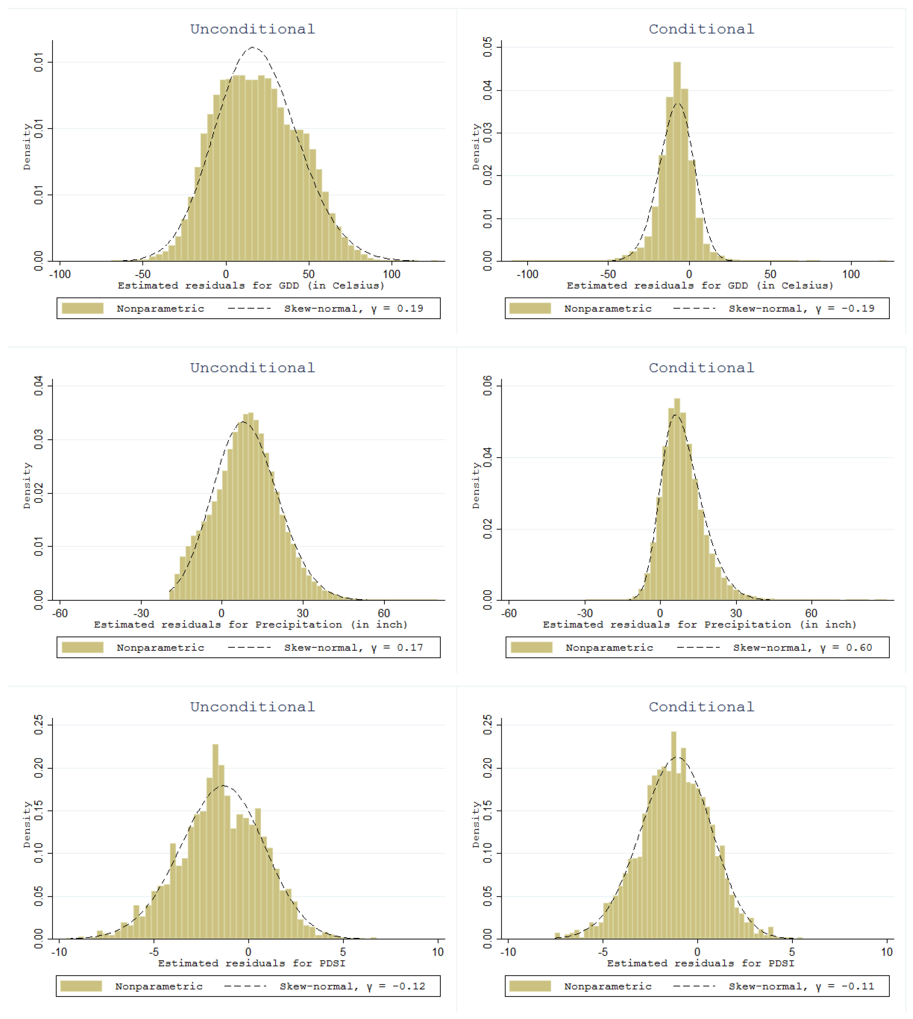
Figure 1 reports residual density estimates using histograms and fitted skew-normal distributions for growing degree day, precipitation, and PDSI (from upper to lower panels). Each graph plots the residual density estimate of fitted values from the skew-normal distribution against the nonparametric residual density, which is estimated with histogram plots. The author first fits a skew-normal distribution estimation and examines the distribution of residuals from its fit. The unconditional residual density estimates of the raw county-level data for the period of 1950–2015 provide evidence that their residual densities expressing departure from normality are not symmetrical. Mean estimates are computed from the formula of the skew-normal distribution given in Equation (1). Note that if we estimated a nonparametric kernel distribution or histogram for the raw data, we would obtain exactly the same shape, skewness, and height for the distribution as in the unconditional case in
Figure 1, except for the location of its mean.
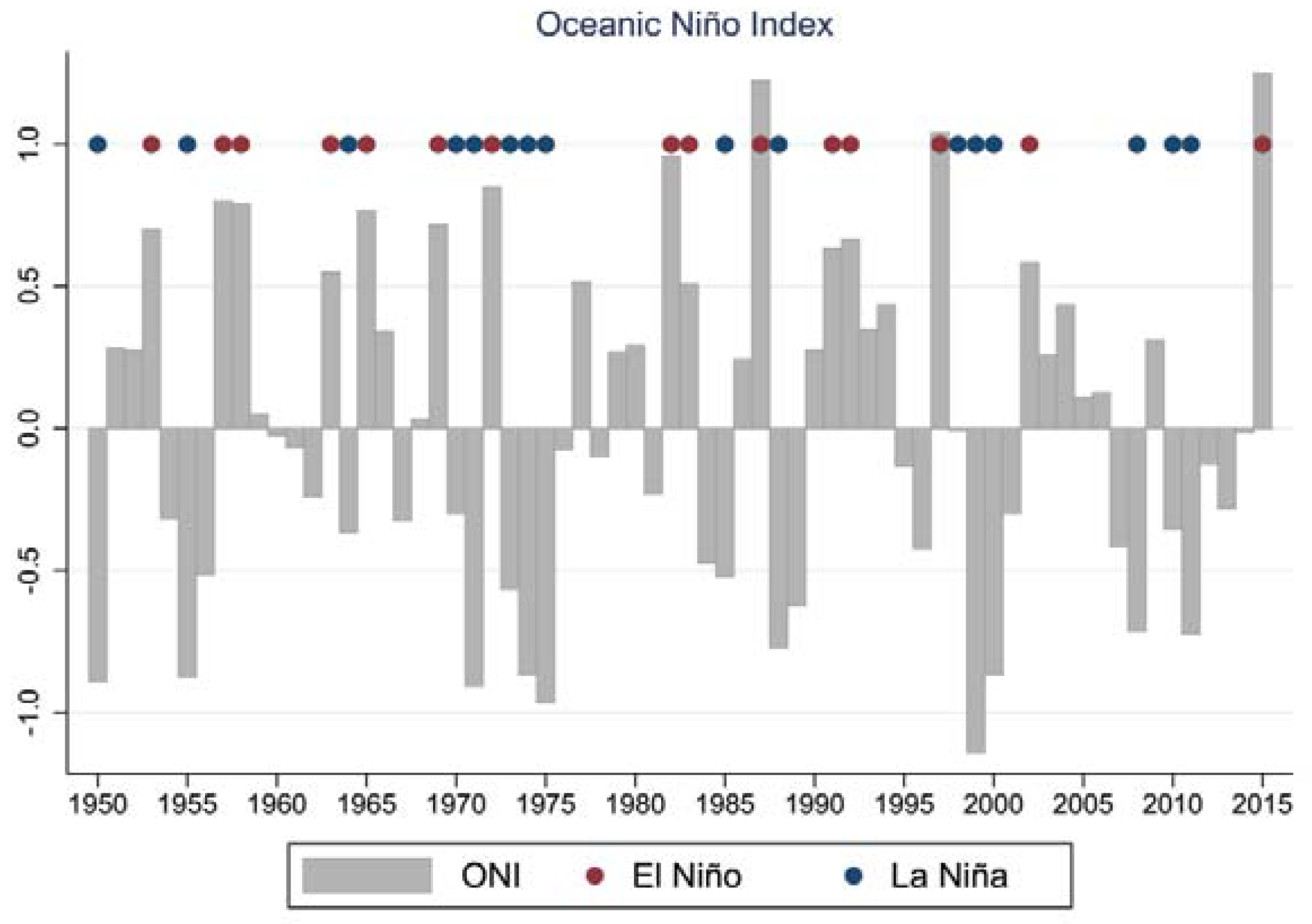
In statistics, the conditional mean or conditional expectation of a random variable is its expected value given that a certain set of “conditions” is known to occur. In this study, the unconditional residuals are simply obtained from the observed residuals that deviated from the expected mean of growing degree day, precipitation, and PDSI. On the other hand, the conditional expectation of growing degree day, precipitation, and PDSI is the expected value of itself given a conditioning set of time and space variables along with the regional dummy variables of El Niño and La Niña, e.g., in its simplest form . Therefore, the conditional residual distribution of the weather variables of interest is the distributional deviations from the conditional expectation controlled for year and county covariates.
From
Figure 1, the conditional residual density estimates from a skew-normal regression controlled for temporal and spatial heterogeneity, with less dispersions after controls, reveal the same results as the unconditional residual density estimates that confirm the skew-normal distributions. Therefore, this empirical evidence provides validity in modeling the skew-normal regression for growing degree day, precipitation, and PDSI.
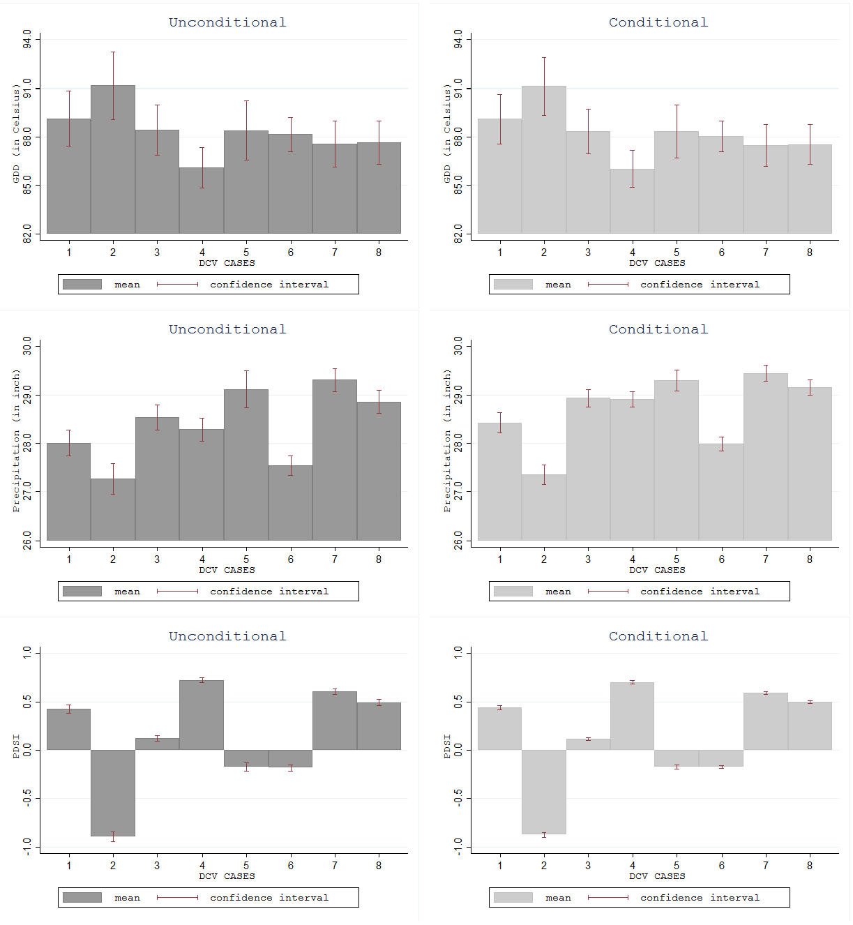
Figure 2 illustrates variations in the mean of growing degree day, precipitation, and PDSI from upper to lower bar graph panels in different DCV phase combinations. The unconditional means are estimated using the raw county-level data for 1950–2015, and the conditional means are obtained from the fitted skew-normal regression with year and county dummy variables. The 95% confidence intervals used here are
, where
is the standard deviation and
is the critical value from the Student’s
distribution with
, which both statistics were calculated with the
effective degree of freedom. The
effective degree of freedom followed [
34] for
, where
is the values of autocorrelations at a lag of one year for each DCV case, as similar to [
35,
36,
37]. The conditional means could be slightly different from the unconditional means especially for precipitation possibly due to the skewness in their distribution. Nevertheless, the estimation results of unconditional and conditional mean are consistent across different DCV phase combinations.
Therefore, the evidence illustrates that the DCV phenomena alter growing degree day, precipitation, and PDSI at the national averages. For example, under the (PDO−,TAG+,WPWP−) phase, growing degree day is highest, precipitation is lowest, and drought is most prominent. Similarly, other DCV phase combinations have different variations of the three weather variables. The ranges which are the difference between the lowest and highest values for growing degree day, precipitation, and PDSI are 5.06 °C, 2.04 inches, and 1.62 PDSI units, respectively.
Furthermore, the sample means of growing degree day, precipitation, and PDSI by DCV phase show that, at the national averages, they are correlated to others. A DCV phase with high (low) average growing degree day tends to have low (high) precipitation and low (high) PDSI. The pairwise correlation coefficient of national averages between growing degree day and precipitation is −0.55, between growing degree day and PDSI is −0.83, and between precipitation and PDSI is 0.58.
State-Level DCV Effects on Climate
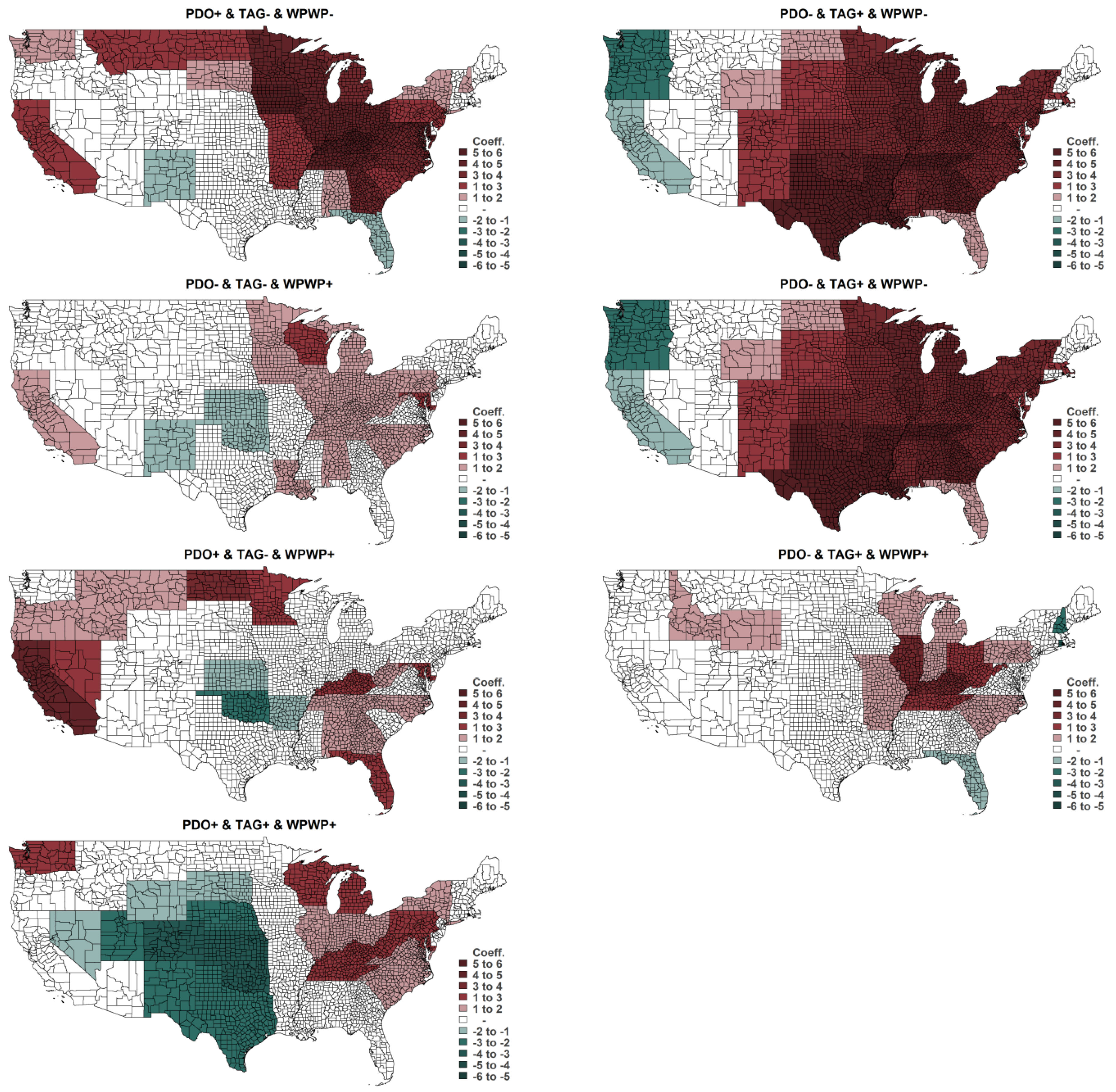
The DCV phase combinations were found to have an influence on growing degree day, precipitation, and drought across the United States. In general, the DCV phase combinations have spatially varying and statistically significant effects for the 48 contiguous states as shown in
Figure 3,
Figure 4 and
Figure 5. Their full results of skew-normal regression models are reported in the
Supplementary Information. The ordinary least squares regression (OLS) estimation results are also available in the table as the reference comparison of estimates. The estimated regression coefficients and their statistical significance from both OLS and skew-normal models are very similar.
The empirical results suggest the skewness in density functions of growing degree day, precipitation, and PDSI; therefore, the skew-normal regression should provide more accurate estimates. The -squared values provide goodness of fit for the OLS regression model as the benchmark indicating how well the linear regression can explain the relationships for the dependent variables such as growing degree day, precipitation, and PDSI with the DCV phase combinations and other explanatory variables. The -squared values for the OLS estimations are 0.9, 0.6, and 0.2 for growing degree day, precipitation, and PDSI, respectively. The -squared values indicated that the observed outcomes of growing degree day and precipitation could be explained well by their estimated regression model. However, low -squared value for PDSI possibly occurred from the fact the PDSI information is state-level, while the county-level data was used. The author made the PDSI regression results available even with low -squared value, because they are consistent with the DCV impacts on growing degree day and, in particular, precipitation. The skew-normal regression has no -squared results, as it is estimated with the maximum likelihood estimation approach.
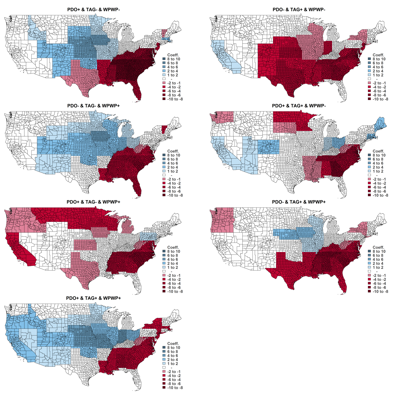
Figure 3,
Figure 4 and
Figure 5 report DCV impacts on growing degree day, precipitation, and PDSI by contiguous state. The figures show the associations with combinations of positive and negative phases of DCV phenomena. Relative to the null-DCV phase combination (PDO−, TAG−, WPWP−), the estimated coefficients presented in these figures are obtained from interactions of dummy variables for DCV phase combinations and dummy variables for contiguous states in the skew-normal regression using annual county-level weather data described earlier. Estimated coefficients illustrated here are only those with 95% confidence with the cluster-robust
p-value < 0.05.
The DCV phase combinations have an influence on growing degree day, precipitation, and drought during the crop-growing seasons in the Corn Belt states and the Southeast states, except Florida, which are the major producers of corn, soybeans, and wheat. The (PDO+, TAG−,WPWP−) phase combination increases growing degree day and precipitation for many contiguous states in the Central and Northern Plains regions such as Iowa, Illinois, Nebraska, Indiana, North Dakota, South Dakota. Furthermore, the (PDO+, TAG−, WPWP−) phase increases growing degree day and drought but decreases precipitation in the Southeast region such as Tennessee, Kentucky, North Carolina, and South Carolina.
However, the (PDO−, TAG+, WPWP−) phase has impacts on increased temperature and decreased precipitation, especially for almost all states in the Missouri River Basin and Southern Plains regions for many major crop-growing states. The (PDO−, TAG+, WPWP−) phase also increases drought extensively in the Southeast and Southern Plains regions except only Florida.
The (PDO+, TAG−, WPWP+) extensively increases growing degree day, decreases rainfall, and increases drought in many contiguous states. The (PDO−, TAG−, WPWP+) phase also increases temperature and decreased rainfall in several states, but the impacts varied by region with lower impacts than the (PDO+, TAG−, WPWP−) and (PDO−, TAG+, WPWP−) phase combinations. All other DCV phase combination impacts are provided in
Figure 3,
Figure 4 and
Figure 5.
4. Discussion
The oscillations in the growing degree day, precipitation, and drought in many contiguous states of the United States reach extreme severity in some DCV scenarios, such as under the (PDO−, TAG+, WPWP−) or (PDO+, TAG−, WPWP+) phase combinations. In addition, other DCV phase combinations have regionally differentiated effects on growing degree day, precipitation, and drought, with both increases and decreases found. The reasons for how the decadal variability indices jointly influence the weather in the United States are unknown to the author, and the unidentified mechanisms underlying in the DCV impacts provide an unsolved problem for future research in atmosphere and climate physics. Nevertheless, this preliminary assessment provides the estimated impacts of the DCV under each phase combination of three indices of the decadal climate variability.
To check the validity of the results, the author compares the estimated DCV effects with those from Mehta et al. (2012) [
18] for the Missouri River Basin region. They found strong DCV phenomena associations with regional temperature and precipitation. Specifically they found that during PDO+, precipitation was above average almost everywhere and temperature was lower than average. In the TAG+ phase, they found precipitation was below average almost everywhere and temperature was increased almost everywhere. In terms of WPWP impacts, they found the effects varied geographically and generally had less impact than PDO and TAG. This study has essentially the same results as in Mehta et al. (2012) [
18] with almost all of the statistically significant terms having the same sign of effects. Collectively, the results in Central, Mountains, and Northern Plains such as Iowa, Illinois, Nebraska, Kansas, Indiana, and others are similar to Mehta et al. (2012) [
18].
This study also reports further the DCV impacts on hydrometeorological variations from other combined DCV phases across the country. The (PDO−, TAG−, WPWP+) and (PDO+, TAG+, WPWP+) phase combinations increase rainfall in a wide area of the corn belt states as similar for the impacts of (PDO+, TAG−, WPWP−). However, some DCV phase combinations also severely decrease rainfall in the Southeast region except Florida in some cases. Given the same DCV phase combination, the results of DCV impacts on precipitation and drought are trivially consistent in most areas.
Essentially, the DCV phase combinations exert regionally differentiated influences on growing degree day, precipitation, and drought in many major crop growing areas such as in the Missouri River Basin and other regions which produce corn, soybeans, and wheat extensively for the United States.
5. Conclusions
An improved understanding of DCV on weather is very important because farmers and policy makers need to know the likely climate trajectory for the coming decades and its impacts for applications to agricultural production and other economic activities.
This study has the same findings for the contiguous states from the Missouri River Basin as in Mehta et al. (2012) [
18], that: (1) during the positive PDO phase, precipitation was above average almost everywhere and temperatures were generally lower than average; (2) in positive TAG phases, precipitation was found to be below average almost everywhere and temperatures increased almost everywhere; and (3) WPWP impacts varied by subarea and had less influence than PDO and TAG in the Basin.
This study extends the results from Mehta et al. (2012) [
18] by reporting that DCV phenomena have regional effects on growing degree day, precipitation, and drought across the United States. In particular, effects are found in the major production areas of corn, soybeans, and wheat, such as the Corn Belt and most of the Southeastern United States. Thus, the empirical results suggest that DCV phenomena could influence hydroclimatic variations, which in turn possibly affect crop production among other sectors regionally across the United States.
There are some limitations in this study. The author used a limited set of years and better estimates might arise under a longer period of study. Future research can cover the increasing effects of anthropogenically forced climate change, variation in solar radiation, and dynamics of jet streams in the climate regressions. Future studies also can cover analyses of DCV impacts on higher moments of the distributions to understand the impacts on variations and skewness of growing degree day, precipitation, and drought. For example, higher variance implies more uncertainty. In terms of skewness, a positive effect in regression coefficient means there is a longer right tail and more concentrated mass of distribution on the left side of the distribution. Thus, there are relatively lower (below the mean) outcomes, e.g., lower level of rainfall or lower PDSI, which means more severe drought.
Despite the limitations, this study adds value to the literature by presenting findings which provide information of DCV impacts on weather in crop-growing seasons that allows adjustments in planning and policy for the United States.


