1. Introduction
In order to have a better understanding of the temperature behavior of the city of Medellín and its metropolitan area in the Aburrá Valley, which is situated in the Andean mountains of Colombia, two different statistical models were developed, which seek to describe and explain temperature increases and variations in this region in the recent years and how human factors influence this. For the models, the studied time range goes from 1995 to 2015.
1.1. Basic Model Description and Objectives
In this paper, the authors have built models to describe the behavior for the temperature of the city from 1995 to 2015. The observation of the temperature shows an underlying tendency to grow in linear fashion complemented by several oscillations that deviate from the linear tendency. Then, to describe these two basic behaviors the authors did as follows: First, a model of temperature changes was elaborated based on global and climate impacts on variations to describe oscillations. Its results are described in
Section 3.1. Second, two models were elaborated to describe the underlying linear tendency: A model that is based on the activities (described in
Section 3.2) and a model based on Energy Balances (described in
Section 3.2).
Modeling here means the elaboration of correlations between global temperature changes and local meteorological phenomena to describe the oscillations of the temperature; and also the elaborations of correlations between indicators of activity and energy generation to describe the underlying linear growth tendency.
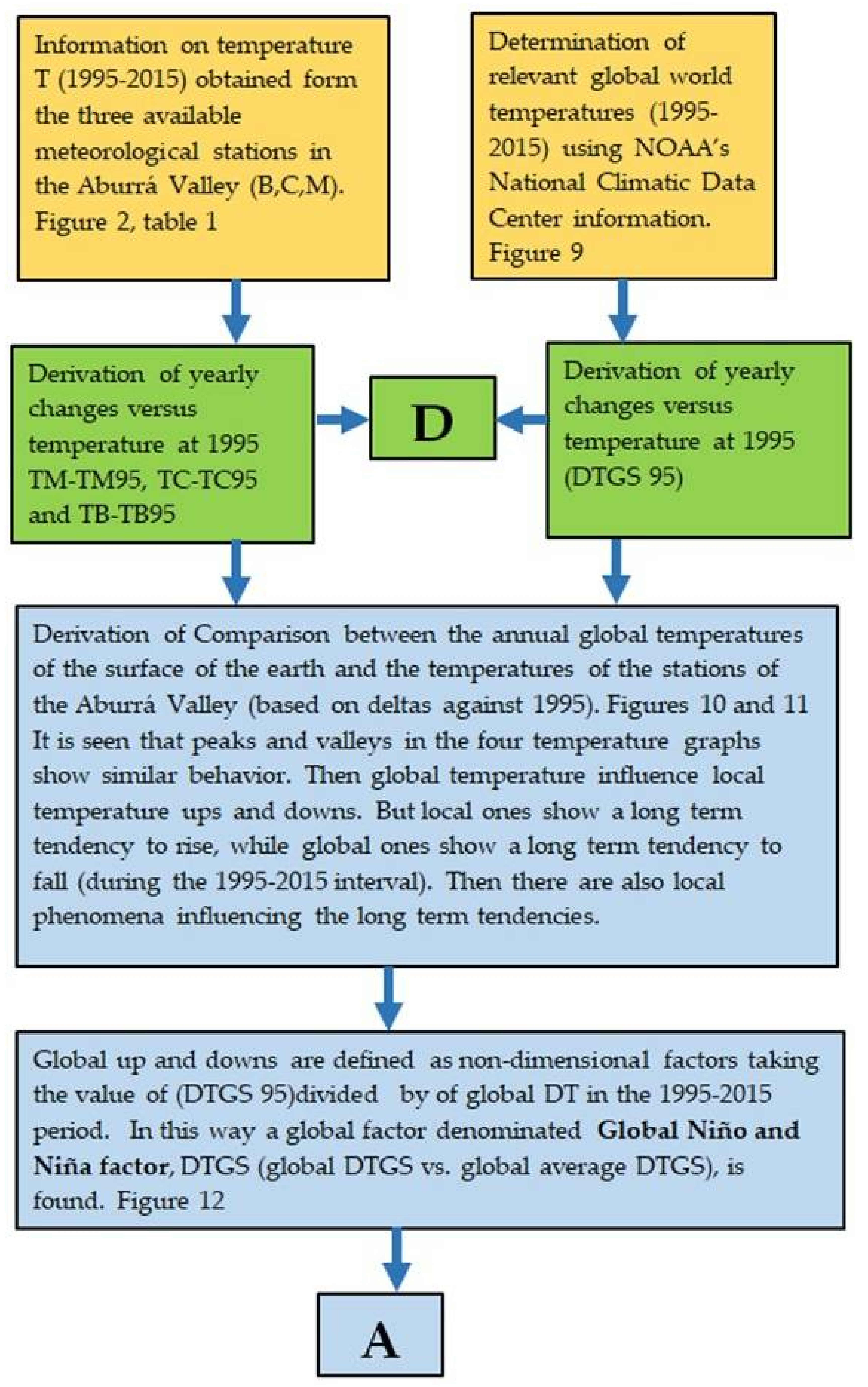
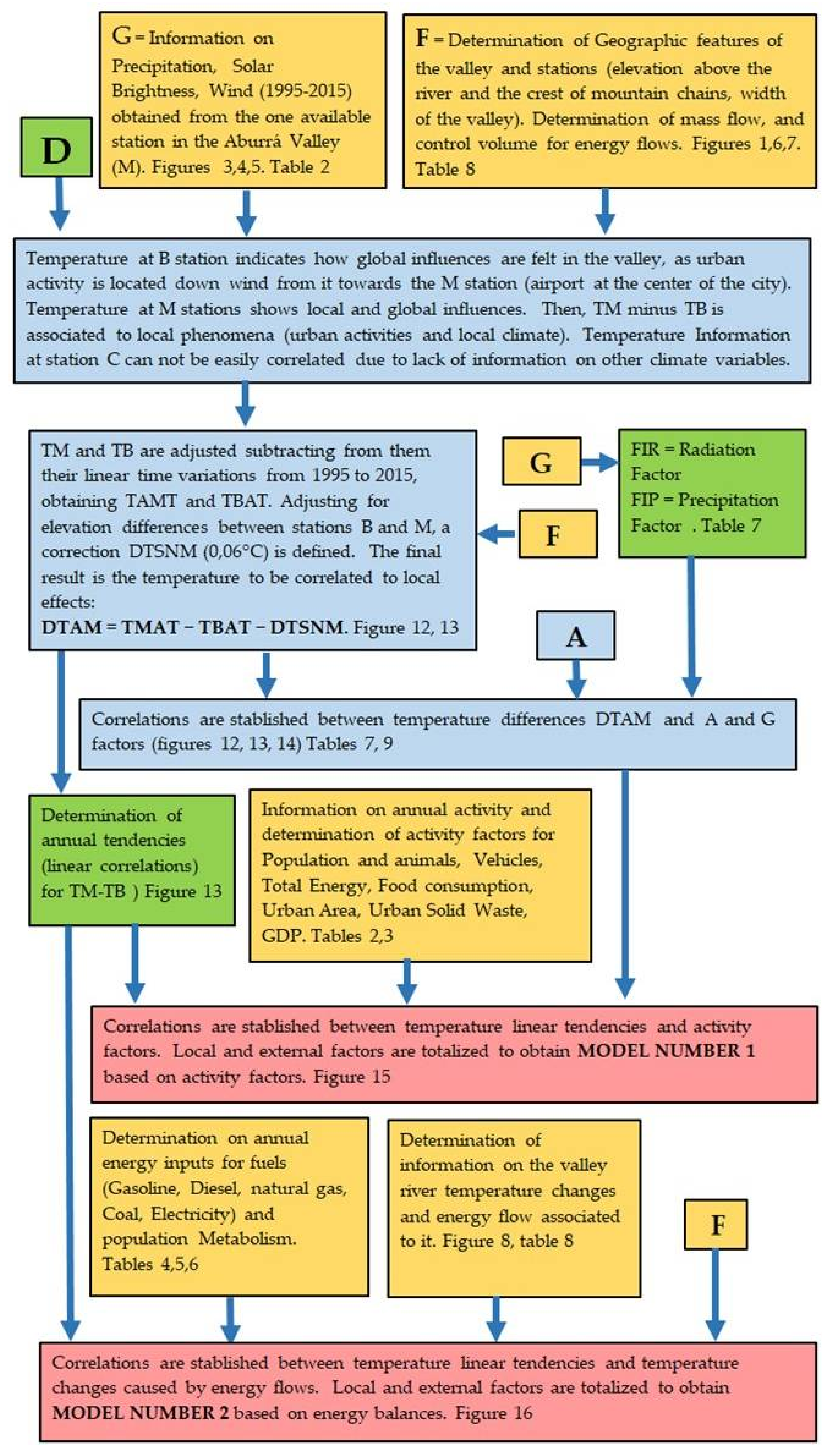
Although the models here developed are simplifications of reality, building them is a somewhat complex procedure, considering the type of variables that influence temperature changes and the fact that a populated valley is subjected to climate, topographic, energy, and activity factors. To facilitate the understanding and logical following of the steps considered in the models, flow diagrams have been prepared and presented in
Figure A1 and
Figure A2 in the
Appendix A.
The model considers two descriptions of the temperature changes. One of them is the tendency of the change, described by means of the linear correlations of temperature data with time; the other one considers the variations of the temperatures in reference to the linear tendencies. For the prediction of the linear tendency, two models are applied: one based in an energy balance that considers the region as a control volume with energy inputs and outputs; and, another one that is based on factors related to human interactions and activities. For both of the models, the goal is to have an approximation to the relative importance of the factors influencing the linear tendencies, but first it is required to understand in which grade they depend on local factors or on external (global ones, such as global warming). So, a methodology was developed to isolate these two major influences. Once the local effects are determined, the goal is to propose some mitigation actions, resulting from the relative importance of the causing factors.
For the case of the variations of the temperatures with relation to the linear tendencies, correlations were developed based on local variations of sunshine duration and precipitation and on global La Niña and El Niño phenomena. The goal was to get an approximation and understanding of those ups and downs in the temperature change, which makes difficult the interpretations of temperature data on the short term.
Another objective is to contribute to a more objective community perception of the climate change in the region, as there is the common perception of the citizens that the inhabited zone of the Aburrá Valley is notably increasing its temperature [
1,
2]. A simple survey of 50 people from the engineering company where the authors work, gives an indication of this perception. They believe that in the last five years the temperature has increased by 1.8 ± 1.3 °C, and that the average temperature of Medellín corresponds to 23.6 ± 2.8 °C. While this shows a good approximation to the average temperature, the increase perceived is grossly exaggerated compared to the reality, as our study shows. It seems that with news continuously mentioning global warming and how the temperatures of the planet are increasing [
3], influences perceptions in the direction the survey indicates. The authors consider that it is important to study these phenomena with an objective view, to really understand what the heating impact of the urban activities on the zone is, as compared to the impact of global warming; and, to find which agents could cause the changes. In this way, citizens can better understand the situation and act in some way to assume the changes and mitigate them. This study is a first step in the direction of examining possible solutions at least at the local level. However, it is believed that the same concepts can be applied elsewhere.
1.2. Urban Temperature Changes. Literature and State of the Art Review
Several scholars around the world have undertaken the task of understanding, studying, quantifying, and seeking alternatives to mitigate temperature changes in urban areas and their areas of influence. There are several types of models that have been developed and presented as tools, and they have a certain similarity with the models presented in this paper. In general, these studies contribute to clarify the variables that are taken into account and their importance in the climate of urban areas around the world. In them, it is noticed the global interest and the actuality of this type of studies.
Several authors seek to characterize urban climate change; Xu et al. [
4] analyzed five long-term meteorological parameters to characterize climate change in the city of Urumqi, China. Huang and Lu [
5] do something similar for the urban agglomeration of the Yangtze River delta, also in China, where with the use of the maximum, average, and minimum temperature observations, a heating rate is determined and compared to the averages, also correlations with factors, such as speed of urbanization, population, and built area are done. Fujibe [
6] analyzes data for 561 stations for 27 years in Japan, where the contribution of urban effects to temperature trends are studied, classifying the stations by the population density around them.
Another field is the Urban Heat Islands, (UHI) studies. For example, Grimmond [
7] seeks to estimate the local effect of cities on climate, as well as their causes, dynamics, and mitigation strategies, Lauwaet et al. [
8] estimate the heat island in Brussels and project it to 2060–2069, by relating meteorological parameters with the UHI. Fuentes [
9] does the same for Tampico, Mexico, characterizing the urban zone and studying the historical macro climate to determine the urban heat island. Stone [
10] makes an analysis for 50 metropolitan areas in the United States and establishes the warming per decade for urban and rural areas and heat island intensity for 50 years. In works like Djedjig et al. [
11], Malys et al. [
12], and Sharma et al. [
13], it is sought to quantify the effect of different land surfaces in urban climatology; the first two study the mitigation of the heat island effect through the use of green roofs and walls, and the latter determines the heating potential of three different land uses.
Most of the reviewed models are based on energy balances, these study the energy flows of the city or account the energy inputs as well as its consumption characteristics. In the work of Kiss [
14] a model of the city of Pécs, Hungary, is presented, which takes into account the energy from heating, electricity, and transport. The study by Chow et al. [
15] estimates the heat emissions of anthropogenic nature, with inventories of population density, traffic and electricity consumption for the city of Phoenix, United States. Song et al. [
16] propose a mass and energy balance model, which evaluates the efficiency of 31 Chinese cities and determine their sustainability; inputs and outputs, such as energy, materials, investment capital, waste, production, and others are considered. In the city of Kiruna, Sweden, Johansson et al. [
17], analyzed the energy model to see the possibility of achieving the performance goals imposed by the national government.
At the national level there are models of determination of energy flows for the city of Pasto by Gómez et al. [
18], they present it as a tool for the planning of a sustainable city. For the city of Bogotá, there is the work of Diaz [
19,
20,
21], in which he seeks to understand the urban metabolism, with the quantification of inputs and outputs of energy, food, and fuels, among others, versus their methodologies of supply, transformation, consumption, and disposal to determine their impact and diagnose the sustainability of the metropolis.
No studies on temperature change that were related to global warming or local activities were found to be applicable to the Aburrá Valley, nor are there studies that use the specific modeling strategies proposed here. The authors feel that their contribution is a valuable one.
1.3. Basic Information about the Studied Region
The region to be studied is the Metropolitan Area of the Valley of Aburrá (AMVA by its acronym in Spanish) that is made up by the municipalities of Caldas, Itagüí, Sabaneta, Bello, Copacabana, Girardota, Barbosa, La Estrella, Envigado, and Medellín (which is the major city, with 65% of the population). This is the second largest metropolitan area of Colombia, after the metropolitan area of Bogotá, the capital city. In total it has approximately 3.8 million inhabitants and urban and rural areas of 102 km
2 and 1054 km
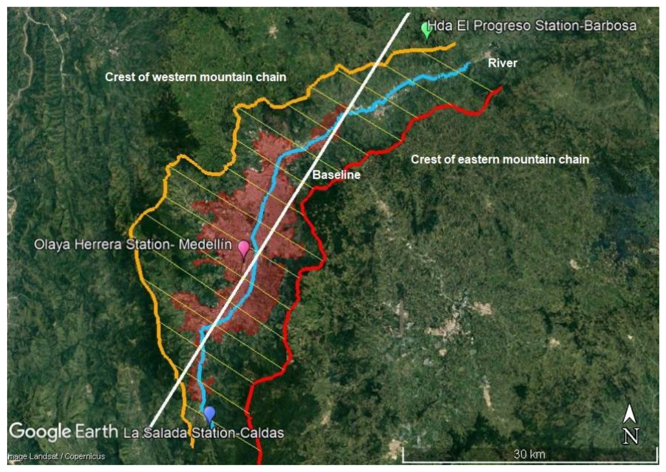
2, respectively. It is located in the center of the department of Antioquia, on the central chain of the Andes mountain range with an average elevation of 1538 m. Located on the tropic; it has quite constant temperatures and small climate variations throughout the year. The area is located in a valley formed by two mountain ranges one to the east and the other one to the west and is crossed by the Medellín river, as shown in
Figure 1.
In
Figure 1, three irregular lines are observed, two representing the crests of the mountain ranges on each side of the valley, and a third one, the river that runs through the middle of the valley. A fourth and straight line is a reference, called “baseline”, which is formed by joining a point in the south west with coordinates 6°02′18.51″ North 75°41′38.70″ West with a point in the north east with coordinates 6°28′47.19″ North 75°24′58.90″ West. This line serves as the axis for the location of distances from the southern to the northern extremes of the valley, and following the direction of the flow of the river. The figure also shows clear demarcated reddish shade urban areas. The position of the three measuring stations is also displayed. These correspond to meteorological measurement points and are the only stations in the region that have the historical data necessary for the study to be performed. The station Hacienda el Progreso is located in Barbosa, which is an area rural in nature and is the place where the winds enter the valley. The station at the Olaya Herrera Airport, which is located in the center of the valley, corresponds to an urban area, and finally, the station La Salada in Caldas, which is a more rural area and at a higher elevation than the previous two, so it is cooler; here, the wind leaves the valley.
2. Data Basis and Methods
The starting point is the collection of data from different sources of information for the diverse sets of variables. These have to do with the climate (local and global), the geography, the river temperatures, the demographic, and economic and activity variables and indicators.
2.1. Information about the Climate
Table 1 shows the mean measured values of temperature in the different stations of the Valley and the precipitation, radiation, wind velocity, and predominant wind direction in the Olaya Herrera Airport station. The variables in this group are thought to have influence or are associated with the temperatures of the city.
The main variable to be studied, temperature, is collected from IDEAM, a reliable data source, “a public institution of technical and scientific support to the National Environmental System, which generates knowledge, produces reliable, consistent, and timely information, on the state and dynamics of natural resources and the environment” [
22] This is the national office responsible of scientific data on climate. Historical data was obtained for the three stations mentioned above. The model considers the average annual temperature.
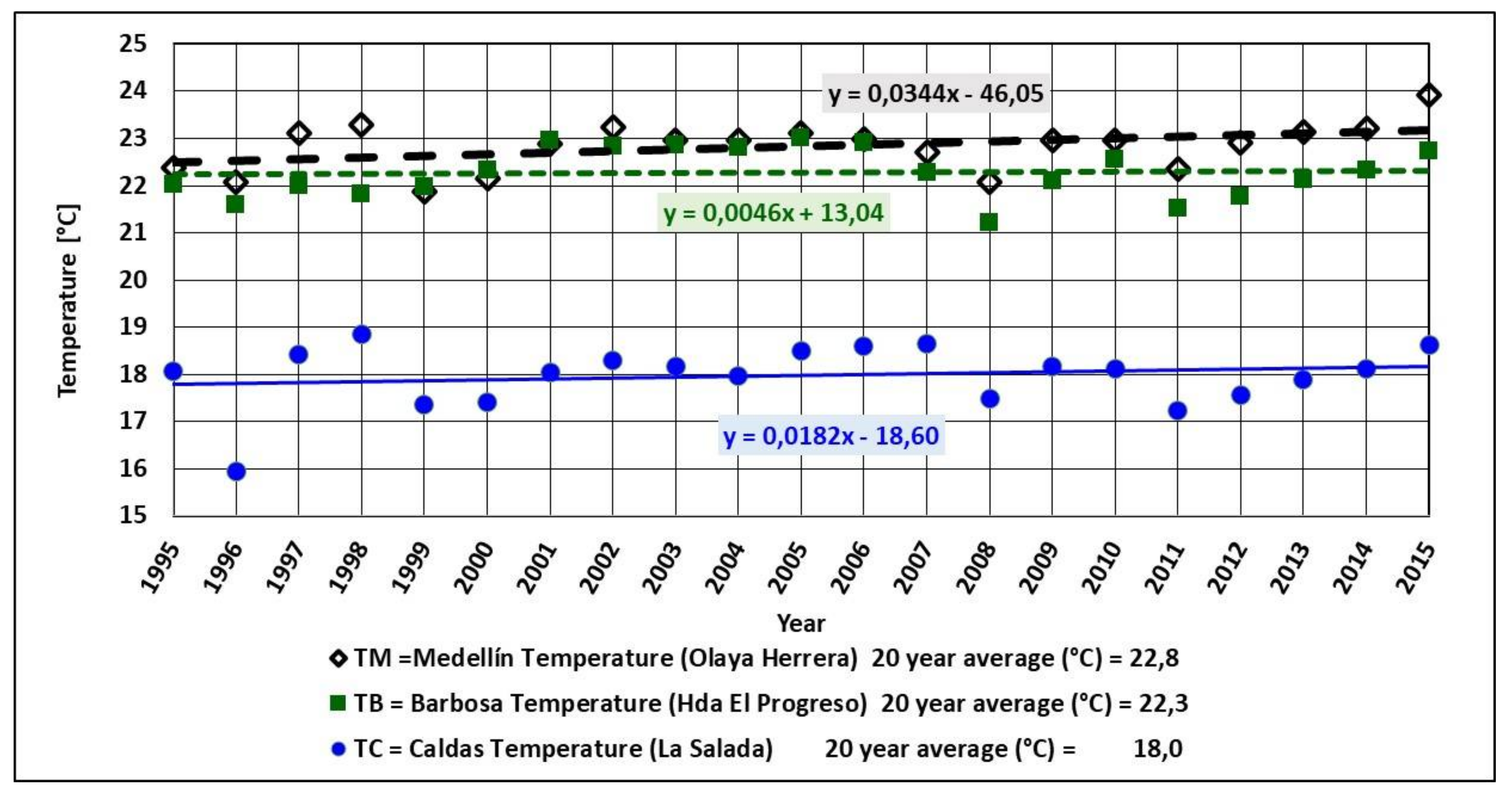
Figure 2 shows the evolution over time for the three measuring stations and their linear adjustment. The shown linear correlations allow for observing tendencies and trends.
As shown in
Figure 2, mean temperatures vary from year to year, with variable behaviors that cannot be easily explained. In any case, it is observed that there are trends. In the case of Medellín and Caldas there is a tendency to growth, while in Barbosa the tendency is to remain fairly constant, with a very small increase. These observations allow for asserting that the causes for the warming in Medellín and Caldas have to do with the human activities in the urban area of the Valley of Aburrá, since these stations somehow have urban nature and receive the influences of the urban activities, stimulated by the predominant direction of the wind, from north to south, from Barbosa to Caldas. In contrast the Barbosa station does not receive this type of influences. But, all of this has to be looked at within the context of geographic variables, especially altitude above sea level of the station, since in the mountainous tropical region temperatures tend to change with elevation.
2.1.1. Temperatures
Figure 2 shows the average annual temperatures for the three stations: Barbosa (Hda el Progreso), Medellín (Olaya Herrera), and Caldas (La Salada), and their respective linear trends between 1995 and 2015. The Medellín station, corresponding to the central zone of the Medellin city, shows the correlation with a higher increase tendency. The Barbosa station, which is situated in a rural area, upwind from the urban areas, shows a very stable tendency, with very small change. The Caldas station, which is situated in an area of mixed rural and urban background and downwind from the main urban settlements, shows a linear increasing trend, but is less significant than the one for the Medellín station.
2.1.2. Annual Precipitation
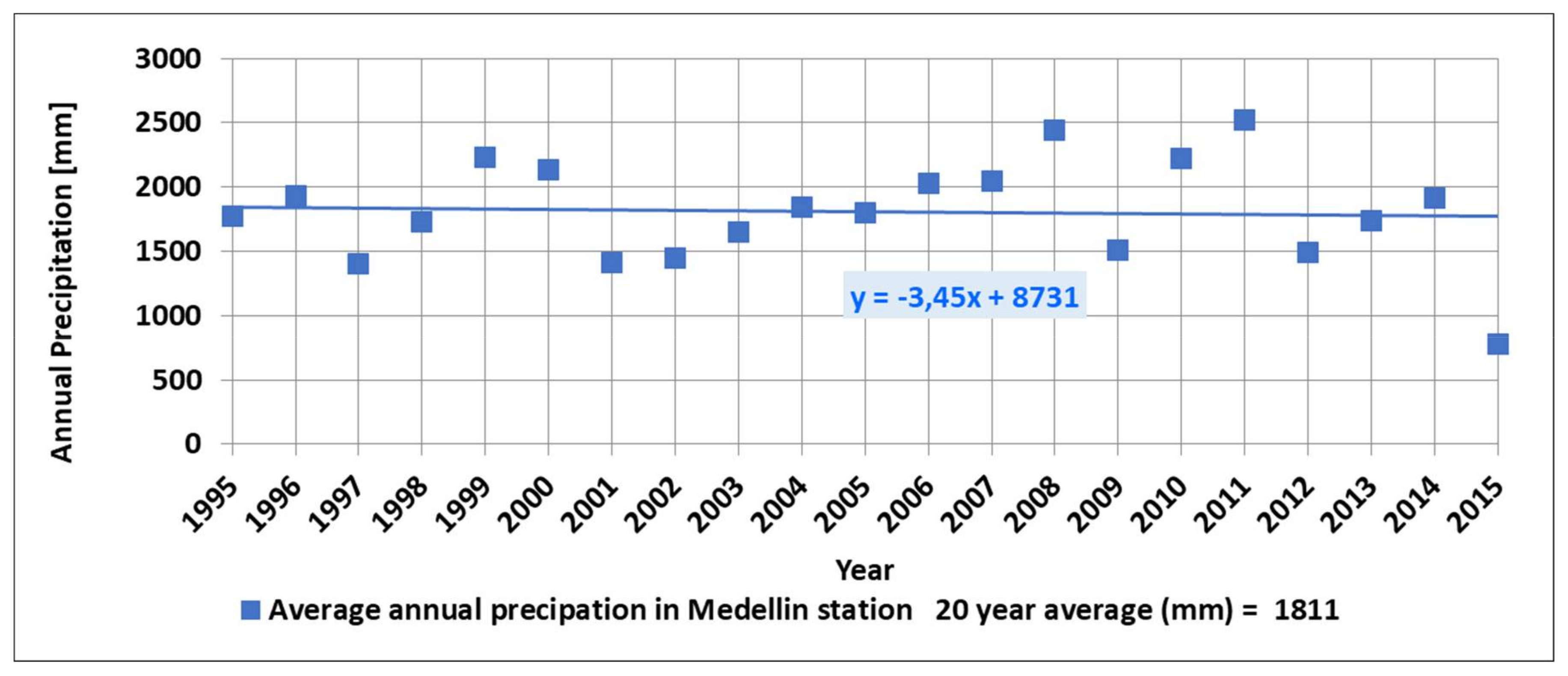
The rains were characterized based on the annual precipitation at the Olaya Herrera Airport station; data is obtained from the IDEAM database. This variable is relevant because it is related to local variations in the temperatures, among others, because of the energy exchanges that are associated with the evaporation of rainwater.
Figure 3 shows the behavior in the study period, significant annual variations are observed, with a relatively stable average trend during the 20 years, around 1810 mm, with a very slight increase in time.
2.1.3. Sunshine Duration
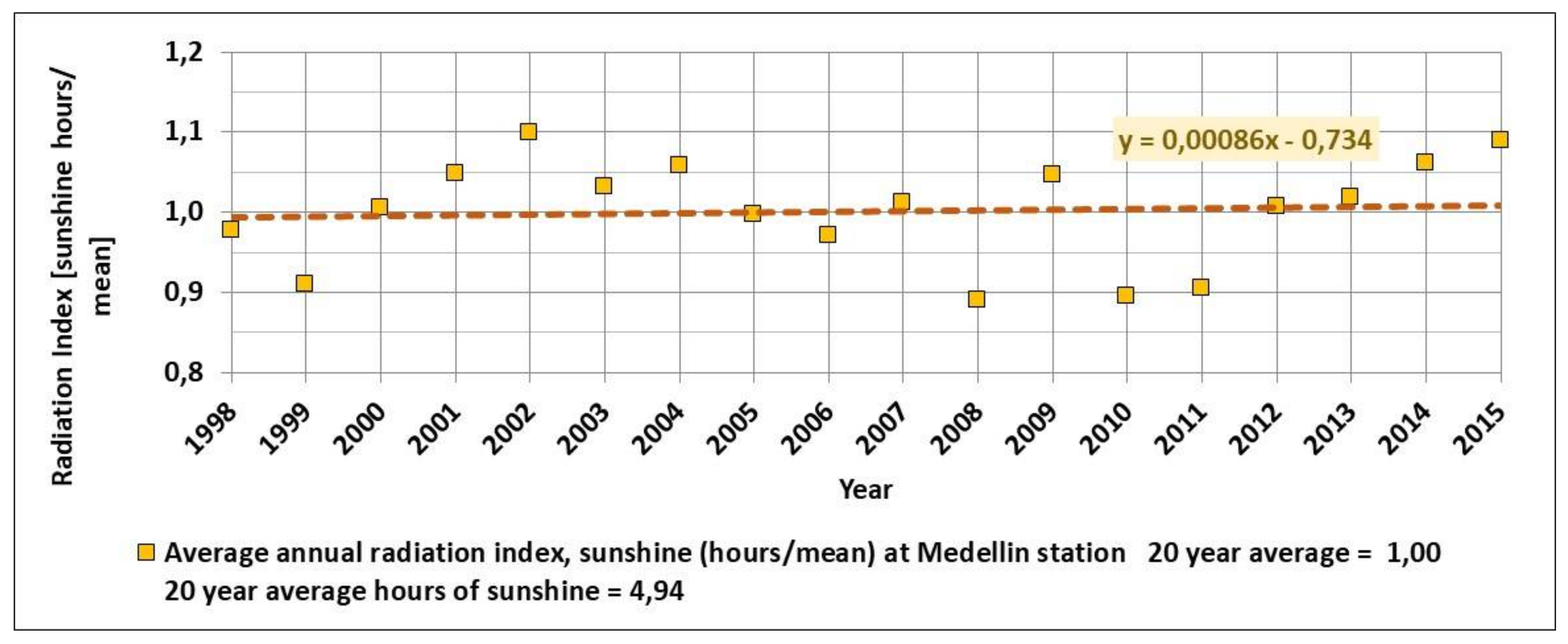
This variable is measured by the IDEAM at the Olaya Herrera station, as the daily hours of solar brightness. For the study, the annual daily averages are considered and have been compared with the average of the study time, which for the period of available measurements (since 1998) was 4.94 h daily. The result of the ratio between the average value of each year and this average of all of the measurements has been taken as an indicator of solar brightness, which is related to solar incident radiation in the region. In
Table 1 the values between 1995 and 1998 were estimated based on a correlation between average temperature and sunshine duration. This variable was taken as indicating solar radiation effects.
Figure 4 shows the behavior
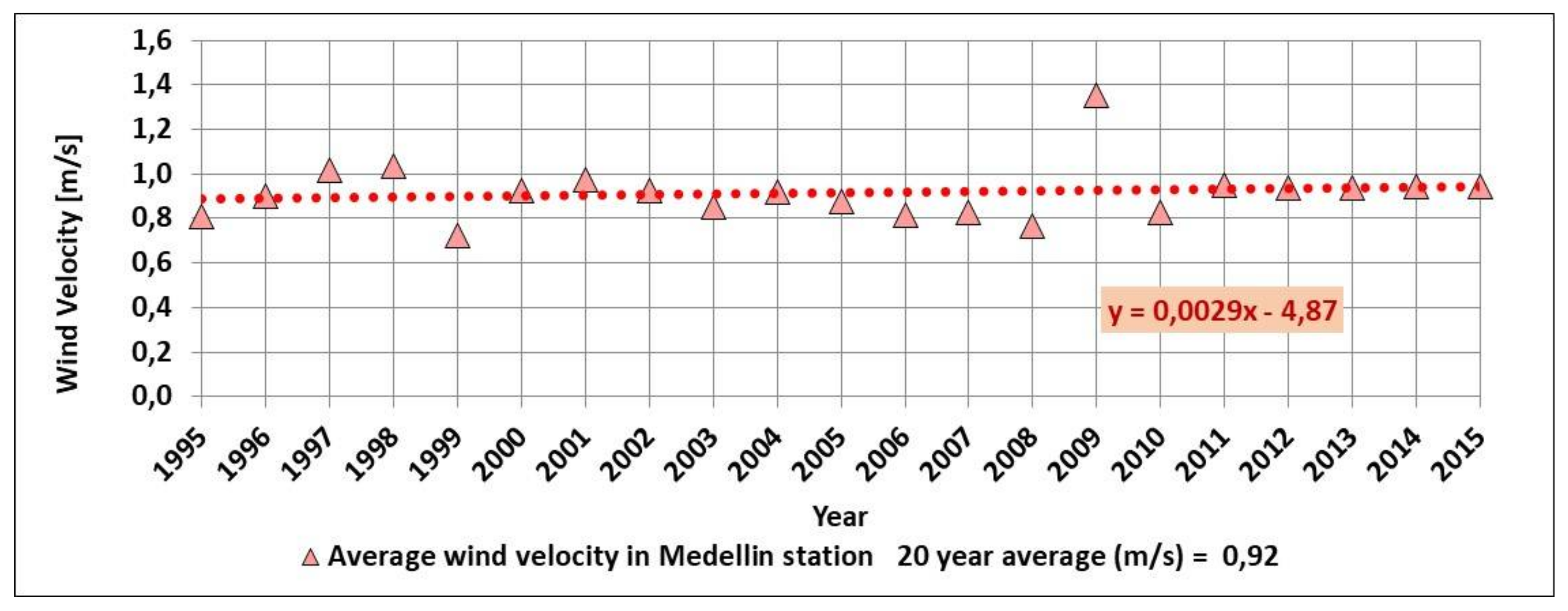
2.1.4. Wind Velocity
The average wind Velocity data for each of the study years was used and obtained for the Olaya Herrera Airport station from IDEAM. Relatively constant annual mean values were observed in the study period, on which the mean value was 0.92 m/s. In 2009, there is an unusual peak of 1.35 m/s, as it can be seen in
Figure 5.
2.2. Geographical Information
Different geographic features have been considered in the study because of their influence on the climate, like elevation above sea level and also their association with urban activities. Likewise, the temperatures and the flow of the river have been taken into account. The river acts as an important sink of heat taking heat losses from activities in the region. This is evident from its temperature, which increases in the downriver northern direction.
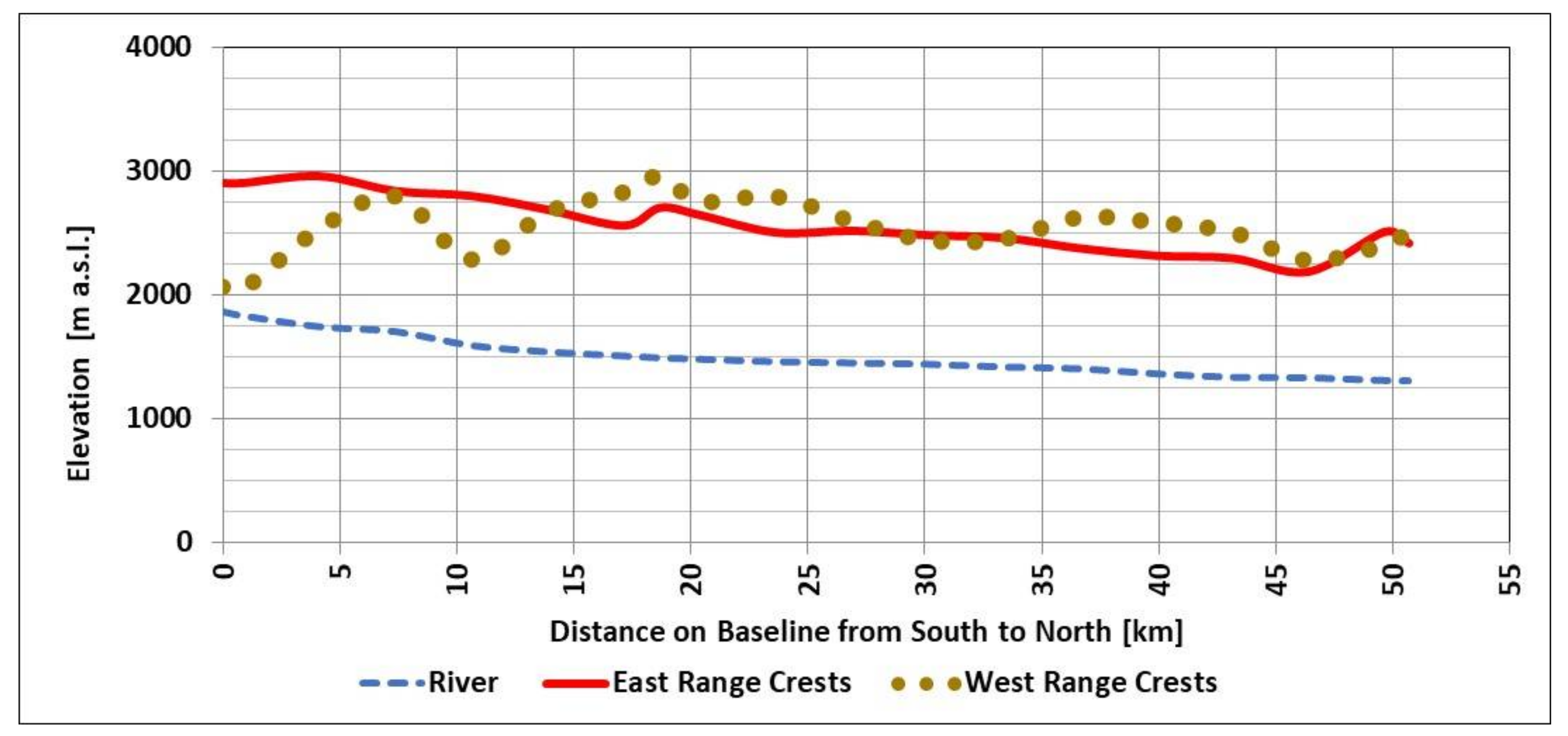
2.2.1. Elevation of the Topographic Levels of the Valley
The elevation above sea level has an effect on the climate in tropical mountain regions. The
Figure 6 shows the geographical situation in the Aburrá Valley, showing the height of the mountain ranges to the east and west of the valley and the height of the river. The graph has taken as a reference the straight line shown in
Figure 1, called baseline. The elevations of the points of the three considered topography lines were taken at points that were joined perpendicularly from each line to the baseline. It is observed that the river descends 552 m in the 51 km length of the baseline, going from 1862 m to 1301 m, with an average height of 1505 m as it passes through the valley. The two mountain ranges have maximum heights of around 3000 m. The average elevation of the eastern mountain range is 2584 m and for the western one is 2529 m. The average elevation in relation to the river is 1078 m and 1024 for the eastern and western ranges, respectively.
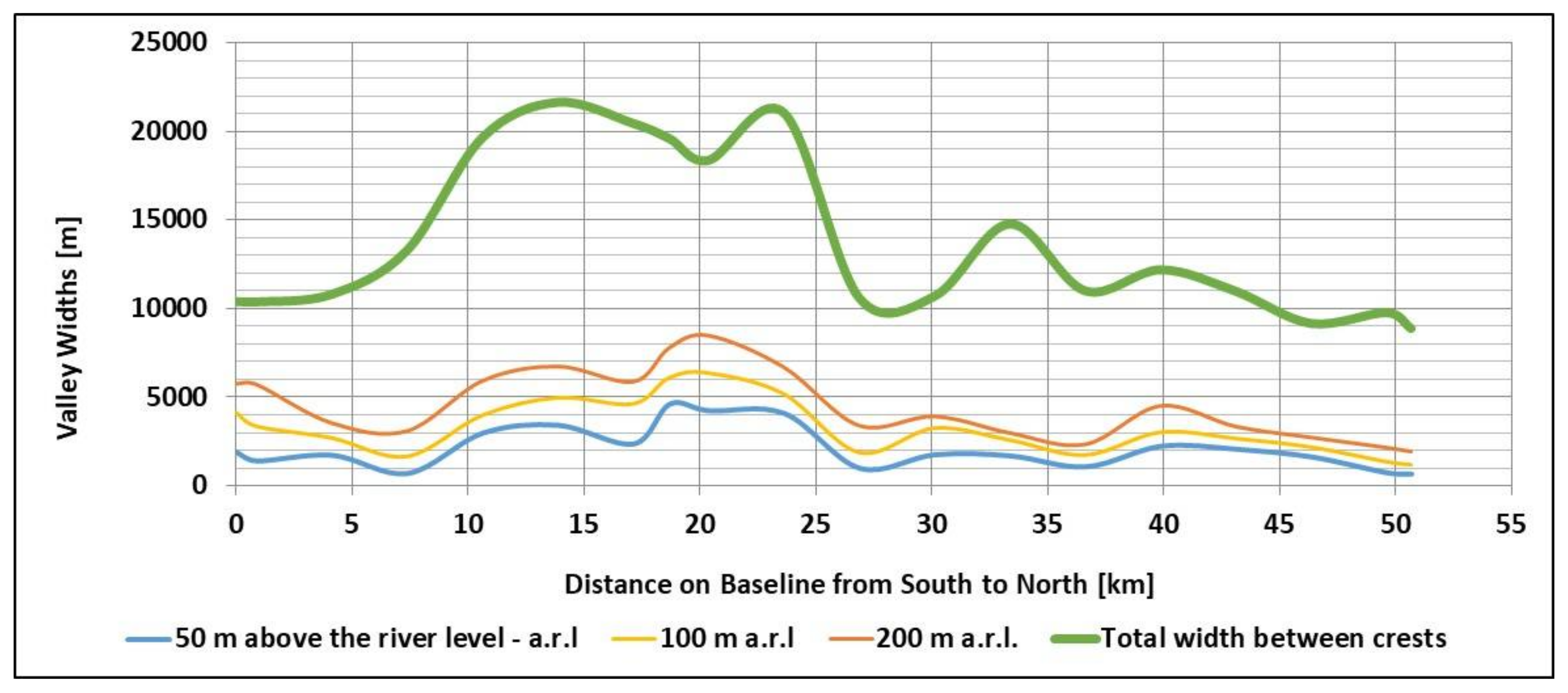
2.2.2. Width of the Valley
An analysis of the width of the valley was made at different elevations, 50, 100, and 200 m above the level of the river, as well as in the ridges of the mountain ranges that form the valley. This was done for different points following the already described reference line that connects the two reference points of the valley from south to north. It can be seen in
Figure 7 that the valley it is relatively enclosed, with total areas of 108 km
2 in the flat zone near the river with less than 50 m above the level of the same, of 166 km
2 in the zone of less than 100 m above the level of the River, of 227 km
2 for the zones of less than 200 m above the level of the river and of 718 km
2 between the ridges of the two mountain ranges that form the valley. The fact that the valley is a box-like system allows for it to be seen as a control volume from the point of view of mass and energy flows, in which mountains act as clear boundaries through which energy and air do not flow significantly. On the other hand, the southern and northern ends are inlets and outflows, especially if is taken into account that the winds have predominant directions from the north, following the direction opposite to the flow of the river.
2.2.3. River Temperature and Flow
There is evidence that the temperature of a water current, under equilibrium conditions, is related to the ambient air temperature, with a behavior that adjusts to a linear trend [
23]. In the case of a river that is contaminated with hot discharges, it is expected that the current temperatures will move away from the equilibrium curves originated in the ambient air temperatures, with temperature differences (delta T) being related to the levels of thermal contamination.
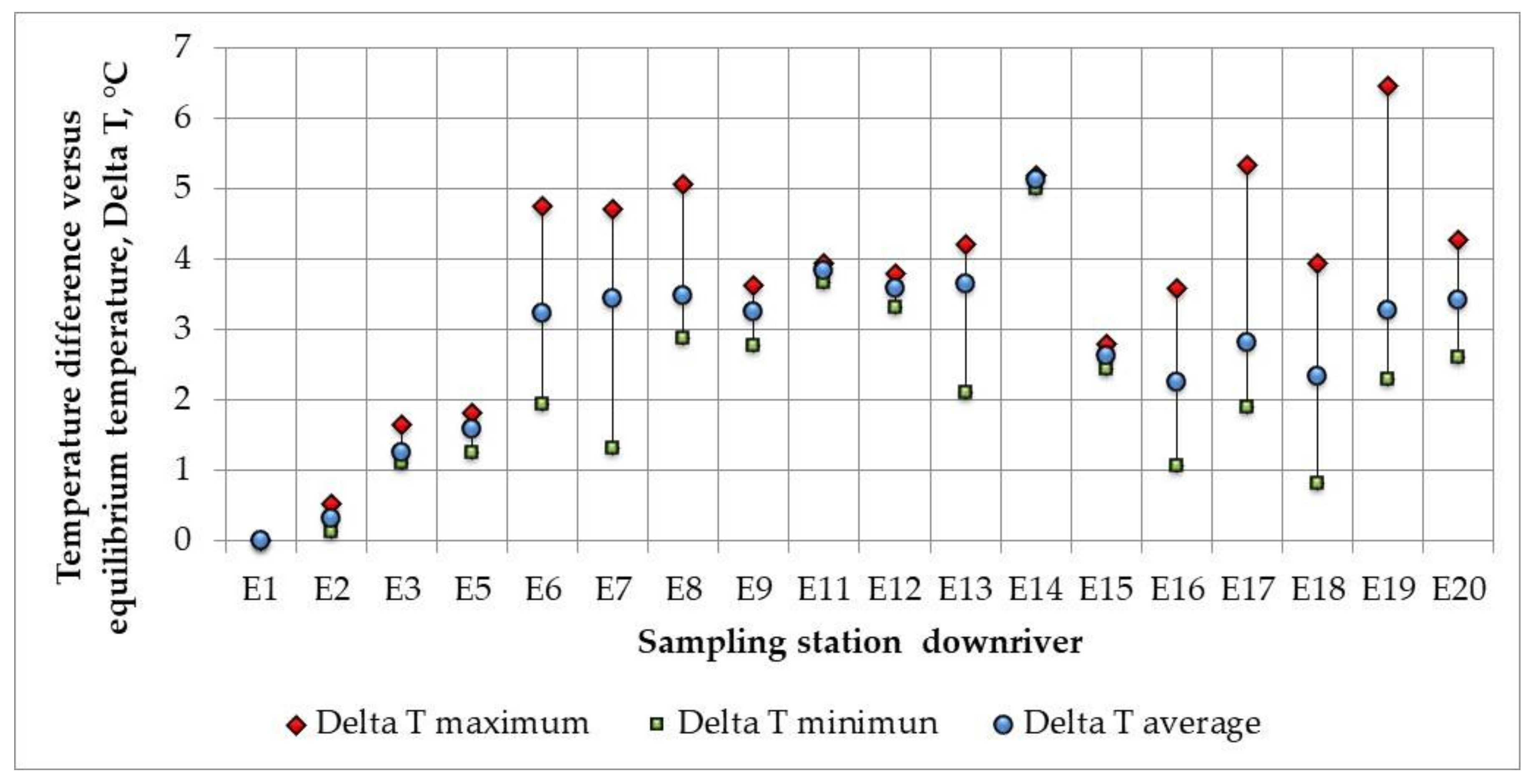
In that way, it has been considered that the river acts as a sink that evacuates part of the heat generated by the energy systems of the region. This means that the river suffers increases in temperature, additional to the ones expected from equilibrium conditions downriver (which depend on atmospheric pressure). An existing study for the Medellin River [
24] is used, which presents these increases in river temperature in zones with urban impact for the year 2006, corresponding to the stretch between stations E2 (called Primavera Station at the south of the valley) and E14 (called the Parque de las Aguas station at the north of the valley, where the Medellín River receives a high flow of water coming from the diversion of the Rio Grande, which causes the cooling of the waters and a new temperature pattern). In
Figure 8, Delta T is the difference between the river temperature and the expected river temperature under equilibrium with the air temperature. The temperature difference was on average 4.5 °C as shown in
Figure 8. Using this information, the magnitude of the heat sink caused by the river in 2006 was estimated, which was 546.4 MW. This magnitude was compared for that year with all of the energy coming from the anthropogenic activities and a factor was found that relates the sink to the total of the energetic contributions. This factor was applied to the other considered years since there was no information for river temperatures in the other years of the study. The authors acknowledge that although this is methodologically correct, it is a limitation in the analysis as compared to the fact that for all other variable considered real annual information has been used. On the other hand, it is proposed that the river temperature profile may be used as a real time indicator of city heat island factor behavior. For this, a temperature measuring system should be put into place.
To elaborate de heat flow calculations for the model, it is estimated that, on average, the Medellín River has a medium flow at the entrance to the AMVA of 1.0 m3/s and that after passing through the urban area it has 30 m3/s; this means a medium increase in flow of 29 m3/s.
2.3. Information on Demographic and Economic Variables
For the modeling, the influence of energy use and human activity has been considered. Demographic variables have been considered, as well as those related to the economic activity of the region. Two models have been developed, one that includes the direct impact of energy variables, and another one that is based on the indirect impact of demographic and economic variables and energy consuming activities. In the second analysis, a change factor was determined to visualize the variables as homogeneous, dimensionless sets. Indexes have been created that correspond to the relation between the real values for each given year divided by the value of the first year of the study, and which quantify the relative growth of each variable.
Table 2 shows the data every five years. The model worked with information for each year. In several cases, such as the information on living beings, vehicles, and energy, values were processed to obtained equivalent men, equivalent vehicles, and equivalent gasoline, respectively, to simplify the modeling. The data used was collected from different public institutions repositories like Banco de la República [
25], DANE (National Administrative Department of Statistics) [
26], Alcaldía de Medellín [
27,
28], and UPME (Colombian Energy and Mining Planning Unit) [
29].
2.3.1. Equivalent Men (Living Beings)
The living beings that inhabit the region contribute with their metabolisms to changing the temperature of the environment. It has been considered that not only are people contributing in this instance, but also other living beings that are in a close relationship with humans, such as pets and domestic rodents (rats and mice). The equivalent men concept seeks to consolidate the number of men, women, children, pets, and rodents in the AMVA region [
30,
31]. The equivalence, shown in
Table 3, was calculated in accordance to the mean body mass of each type of living being in comparison with respect to an adult male weighing 69.1 kg [
32]
2.3.2. Food
This indicator estimates the amount of food consumed by the AMVA inhabitants per year, but it is limited only to humans, the feeding of pets, and other living beings is not considered. For calculating this indicator, the change over time in food intake per person [
33] and the population are considered [
34].
2.3.3. Urban Solid Waste
It is considered that the amount of waste that is generated by the population has influence on the heating of the city, since it is an indicator of the consumption habits of a society and its sustainability. The data is taken from a projection made by the AMVA for the formulation of the integrated regional solid waste management plan [
35].
2.3.4. Constructed Urban Area
The built area of the city is estimated; here a known value reported in a given year is taken into account [
25]. Starting from this value and an annual indicator of the new constructed area, the total constructed area is estimated. This indicator is important since the built areas have a negative impact on the temperature change (causing it to raise) unlike the green areas and parks; these green areas absorb CO
2 and heat, so that as the urban area increases, this ecosystem regulation service is somehow lost.
2.3.5. Gross Domestic Product—GDP
This is an indicator of the total goods and services produced by AMVA annually; it is a representative value of the productive and services activity of the city [
25].
2.3.6. Equivalent Vehicles
To calculate this indicator, the equivalence factors are found between a light vehicle (automobile) and the other considered vehicles. These equivalences have been estimated based on specific average consumption and daily activity time, for each type when compared to a normal automobile.
Table 4 shows the used equivalence factors.
2.3.7. Fuel Consumption in Terms of Equivalent Million Gallons of Gasoline
This is an indicator of the city’s energy consumption, since fossil fuels and electricity are counted here. The equivalence is done in relation to the calorific power of each energy source, as seen in
Table 5. This indicator can quantify better the influence of transport and energy consumption, because even though the number of vehicles increases, technologies evolve and have better fuel yields, with each time requiring less energy per unit distance. The consumption data was obtained from different Statistical Bulletins of Mines and Energy done by UPME [
29]
Based on the variables that have been described, a model for the annual behavior of the temperature has been developed, which includes the direct impact of energy variables and the indirect impact of demographic and economic variables.
2.4. Information on Energetic Variables
A second model has been developed from a purely energetic point of view, based on energy inputs and outputs. For this, the average energy fluxes (
Table 6) have been considered.
According to the previous table, the region receives a total energy contribution that currently exceeds 3000 MW. This contribution essentially dissipates into the medium, even if it is useful energy, since eventually it will generate heat, friction, noise, and other dissipative forms.
2.5. Dimensional Adjustment and Treatment of Variables
2.5.1. Transformation of Temperatures
As shown in
Figure 2, temperatures at the different points in the metropolitan area have different behaviors. For the case of Barbosa (Hda. El Progreso), the temperature shows relatively moderate variations in the 20 years of the study. In the case of Medellín (Olaya Herrera) and Caldas (La Salada), a variable but gradual warming is observed, being more prominent in Medellín. This warming is considered a result of the regional anthropogenic reasons treated in this model. However, it is clear that there are other causes that must be taken into account.
On the one hand, there are the impacts of phenomena of a global nature, which in principle are distributed all around the planet, with certain geographic variations. Global delta temperatures are taken from the information provided by American National Oceanic and Atmospheric Administration (NOAA’s) National Climatic Data Center [
36] and are defined as the difference between Global annual temperatures of the earth’s surface and the temperature average 1901 to 2000.
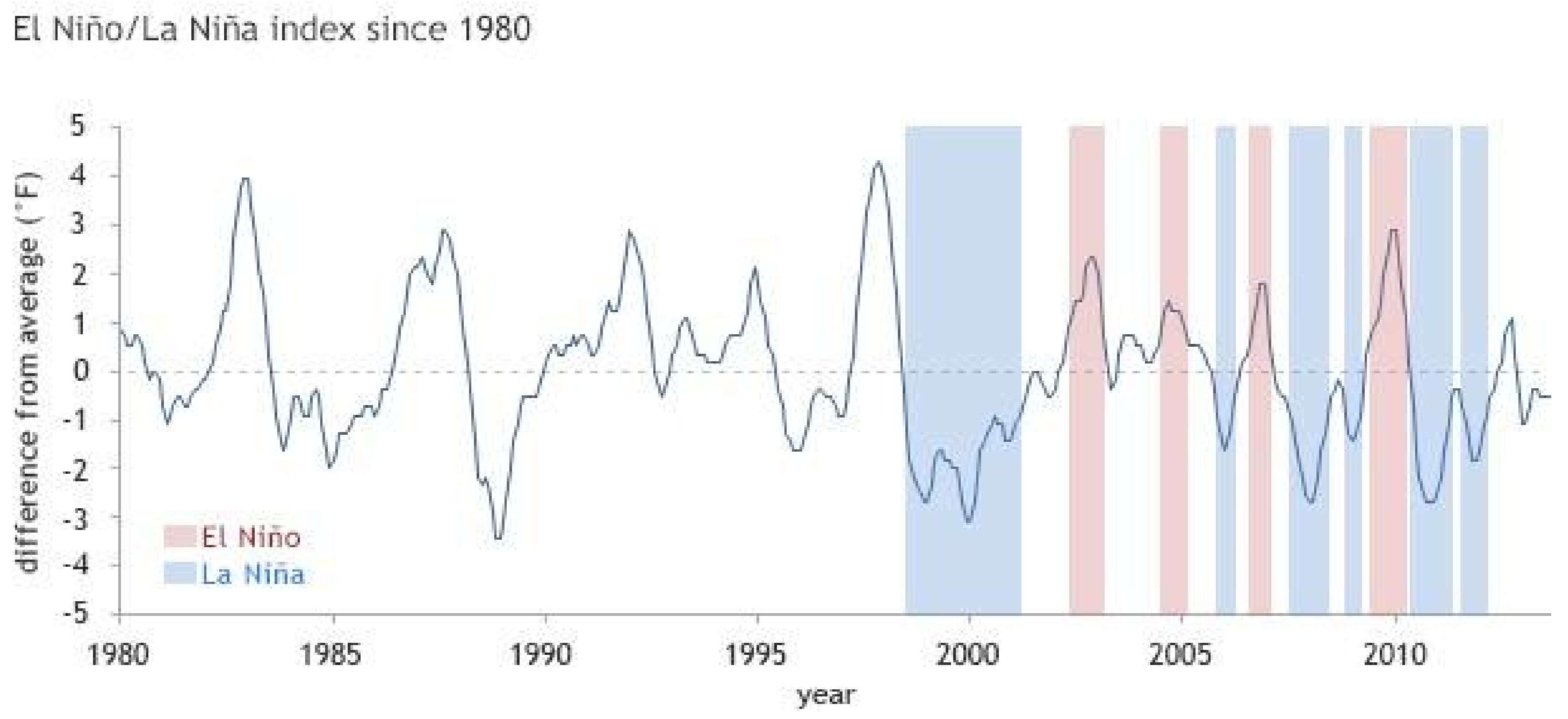
Figure 9 shows this data provided by the NOAA’s National Climatic Data Center, with global temperatures of the surface of the earth, compared against the average between 1901 and 2000 (dotted line passing through zero). The impacts of the Niño (increases) and the Niña (decreases) phenomena are observed. Niña and Niño are names customarily used for these warming and cooling periods. From 1995 to 2015, on average, an increase is not observed, but rather some decrease is noted.
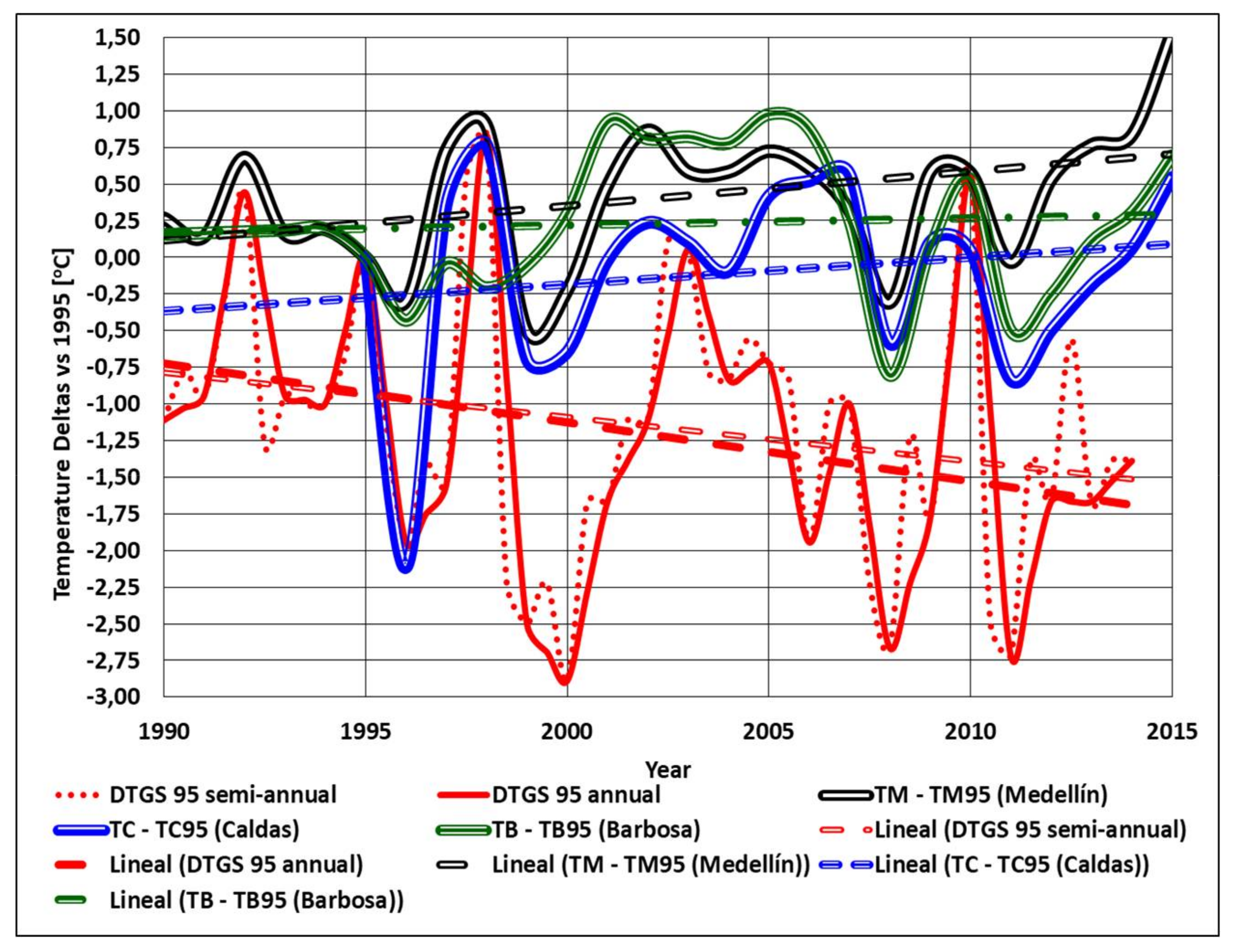
Figure 10 shows the behavior of such global temperatures when compared to those of the studied region in the Aburrá Valley. For this purpose, the data has been processed in the following way:
After converting the global delta temperature from °F to °C, the information was digitized to semester and annual values, from which the data of 1995, the first year contemplated in our study, were subtracted. Thus, DTGS 95 annual and DTGS 95 semester (semi-annual) curves were obtained.
The three annual temperatures of the region, Barbosa (TB, Hda. Progreso), Medellín (TM, Olaya Herrera) and Caldas (TC, La Salada) were taken, and their average values in 1995 were subtracted of each, thus obtaining the TM-TM95, TC-TC95, and TB-TB95 curves.
Figure 10 clearly suggests that the impacts of the Niño and Niña phenomena (associated with up and down changes) are related to the temperature oscillations for the three stations in the region. Such oscillations follow quite well those of global temperatures. However, trends, as seen in linear adjustments, differ from global phenomena to local phenomena. This is probably related to the local behavior of air masses in a relatively long, narrow and enclosed valley between two mountain ranges with 1000 m height, valley in which the urban activity of nearly four million people has a significant impact.
Because the anthropogenic factors tend to grow with time continuously, without major oscillations, it was postulated that they are related to tendencies in the temperatures, as indicated by their linear correlation with time (
Figure 2). The differences between the actual temperatures and the linear correlation, then, are caused by non-anthropogenic nature effects.
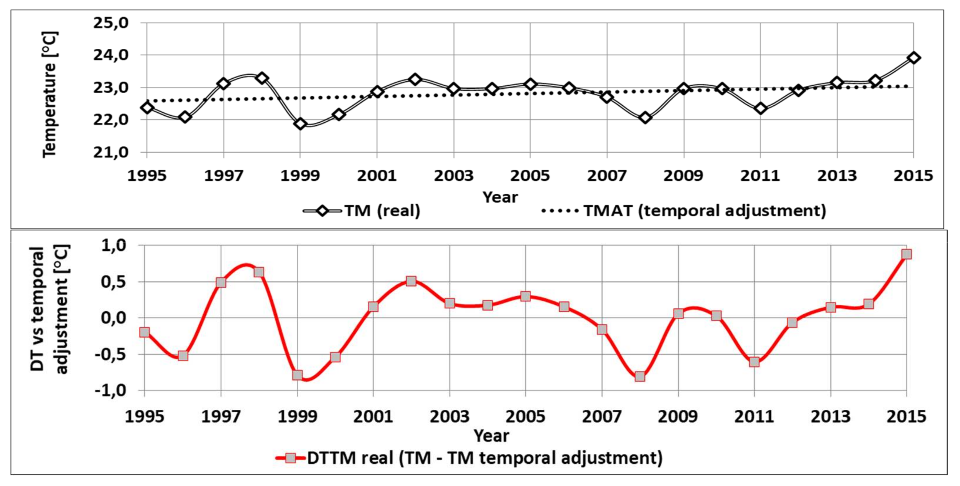
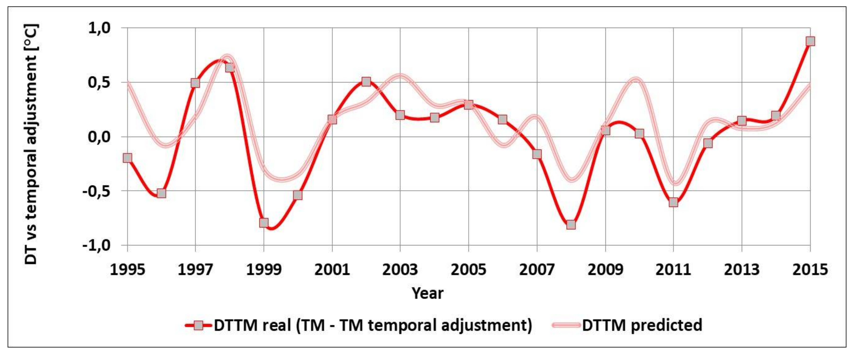
Figure 11 shows the actual Medellín station (TM) temperatures, their linear correlation (TMTA, TM temporal adjustment), and the deltas of temperature between the real temperature and its time adjustment for Medellín.(DTTM) (defined as DTTM = TM − TM temporal adjustment).
It was postulated that such deltas (DTTM) depend on phenomena that are not anthropogenic. For this case, these non-anthropogenic phenomena are, on the regional scale, the local climate influences, taken here as the other major variables besides temperature: average annual rainfall and average annual radiation, and, on the global scale, the universal phenomena of the Niño and Niña, as noted in
Figure 9 and
Figure 10.
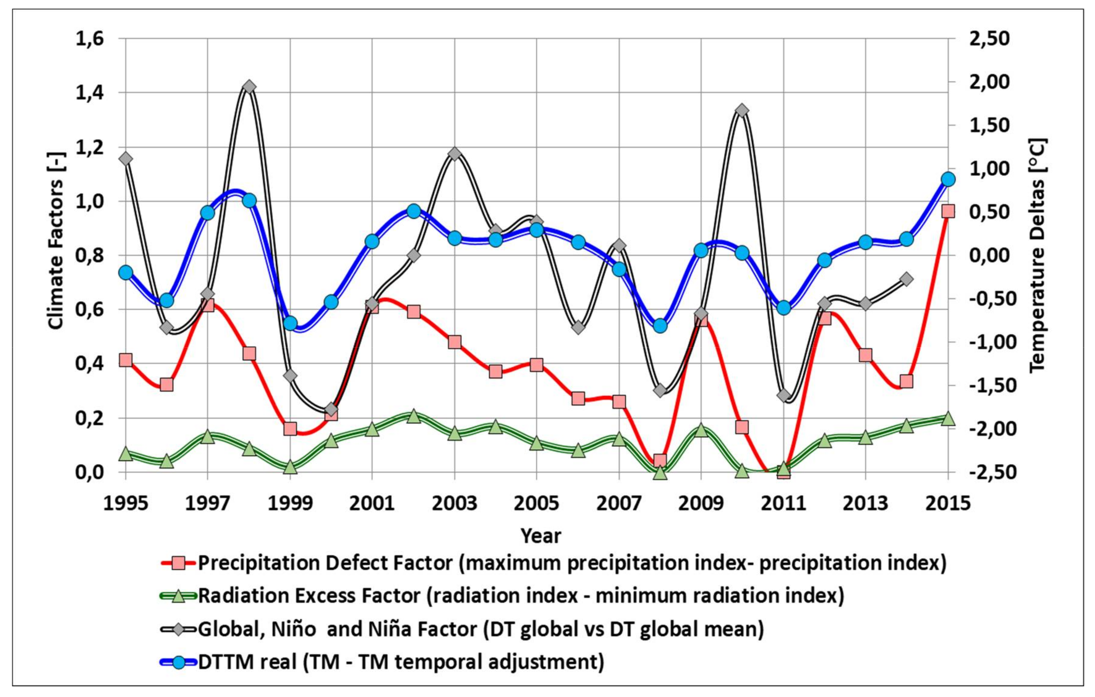
Global Niño and Niña factor. DTGS (global DTGS vs. average global DTGS), taken from
Figure 9 and
Figure 10.
Radiation excess factor (radiation index—minimum radiation index). The radiation index has been defined as the annual sunshine hours divided by the average annual sunshine hours in the studied period. This average value was 1800 h per year. The factor is calculated by subtracting from the annual index the minimum registered index (0.86), which occurred in the year 2008 with a total of 1599 h.
Precipitation defect factor (maximum precipitation index—precipitation index). The precipitation index has been defined as the annual precipitation value in mm of water, divided by the average annual precipitation in the period studied. This average value was 1811 mm per year. The factor is calculated subtracting the maximum recorded index (1.39), which occurred for the year 2011 with a total of 2518 mm, from each of the annual indices.
Figure 12 show the behaviors of DTTM and the said indicators of radiation, precipitation and global phenomenon.
Figure 12 clearly suggests that the impacts of the Niño and Niña phenomena, the Radiation factor and the Precipitation factor, and their up and down changes are related to the temperature oscillations.
Table 7 shows the obtained correlations that can be considered as significant as they have high correlation factor. They are therefore used to predict annual temperature behaviors with relation to DTTM variations against the annual linear adjustment.
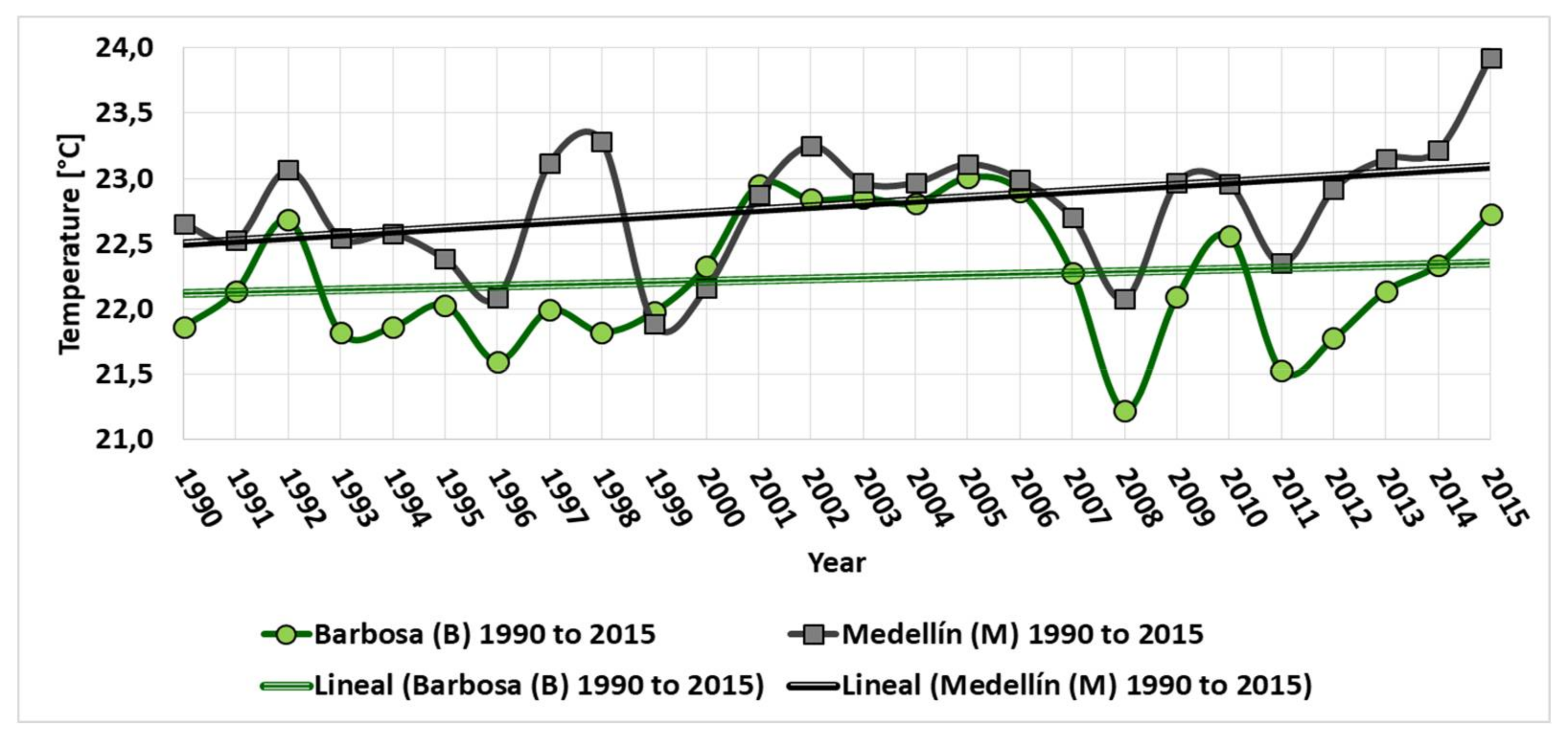
To better understand the changes over time already presented in
Figure 2, the temperatures for stations M and B between 1990 and 2015 are shown in
Figure 13. This shows more clearly that the changes in Medellín are greater than the time changes in Barbosa. A first important consideration was to assume that the change in temperatures in Barbosa corresponds to impacts that are attributable to the mixture of global and local climatic impacts and not to impacts of the activity of the region, this taking into account the situation of such a station in the rural north of the valley, and the predominant direction of the winds, which go from north to south. These two facts indicate that the Barbosa station is not affected by anthropogenic activity.
A second consideration is to assume that the difference between the temporary temperature adjustments of Medellín (TM) and Barbosa (TB) is due to human activity in the region. This activity generates:
Continuous and increasing heat emissions, which origins increases in the temperature of the air passing through the urban area.
Changes in patterns of heat exchange and absorption and emission of solar radiation. For example, increases in the constructed area and in the corresponding circulation surfaces, ceilings, and walls result in changes in surface emissivities and changes in absorptances and reflectances.
Secondary reactions involving the presence of atmospheric agents and pollutants, which supply and consume reaction energies and change in the parameters of absorption and emission of radiation. A value of 0.06 °C (DTSNM) has been discounted from the linear adjustment of temperatures in Medellín (TMAT) and Barbosa (TBAT), considering that station M is at 1490 m above sea level and the station B is at a slightly higher elevation, 1500 m above sea level. In this way, based on time, the temperature difference due to the activity has been constructed as indicated by (1). This DTAM difference is the one to be modeled.
2.5.2. Indexing of Activity Indicator Variables
As already mentioned, indices have been created for the different variables, which correspond to the relation between the real value for each year divided by the value for the first year of the study (1995). These indices also quantify the relative growth of each variable.
2.6. Establishment of Correlations for the Models
Two models of linear nature are made to approximate the modeling of temperature increases as a function of the considered anthropogenic activity factors. The first one based on the factors of human activity and the second one based on inputs and outputs of energy to the mixture zone of the atmosphere of the Aburrá Valley.
The first model assumes that the DTAM temperature changes are the result of a linear combination of the indexes of the activity indicator variables.
where
FAi is the activity influence factor
i and
IAi is the annual activity index
i.
In this model, the dependent variable (left side of Equation (2)) is the linear trend to be modeled. The right side of Equation (2) constitutes the modeled situation as the combination of a group of independent variables with their annual values. To find the influence factors for each variable an Excel Solver routine was used and executed 10 times minimizing in each occasion the average of the absolute values of the annual error (this error was obtained when comparing real DTAM against modeled DTAM), changing the initial values of the assumed factors in the interaction, so that different results are obtained each time. At the end, the obtained factors are averaged.
It is important to understand that this is not a closed problem and that there are multiple combinations that approach the real value of DTAM. There is a high number of parameters in comparison to only 20 years. Because of this, there is no pretense to demonstrate the validity of the obtained linear regression, except inasmuch as the model fits the observation reasonably well permitting a useful approximation to the influence of the studied activity factors, which can be used to propose recommendations such as the ones expounded in this work.
The second model is based on an energy balance in which the energy inputs described in
Table 6 are considered. The heating that the Medellín River suffers due to the activity while passing through the region has been considered in the model as an energy output. A control area has been considered, the width of this area corresponds to an average between the medium width of the valley at 50 m above the river level from Barbosa to Medellín stations, and the width between the mountain ranges at the mixing height; the height of the control volume was chosen, such that it gives a good fit of the model.
Table 8 shows the values for these variables.
The energy balance is described by the following expression:
where:
Qin: Annual energy input to the Control Volume. Comes from the energy sources.
Qout: Thermal energy output that leaves the control volume through the river.
m˙: Air Mass flow that goes through the control volume.
Cp: Specific heat of Air.
∆T: Air temperature change suffered by the air traveling between the ends of the control volume.
For the annual energy input, a percentage of the total energy of the entire Aburrá Valley was considered, when considering that the temperature change occurs up to the Olaya Herrera station. This percentage is proportional to the distance in the central axis from the north to the Olaya Herrera station, as compared to the total distance between the two ends, Caldas and Barbosa, obtaining a percentage of 60.17%; this considers the preferential direction of the wind, from north to south. As for the output of energy carried by the river, a 39.43% of the same (100–60.17)% is considered since the River drags energy in the opposite direction to the wind, from south to north.
In order to estimate the annual average mass flow, the average wind speed in the mixing zone, which was estimated at 2.64 times the velocity at the surface, was multiplied, by the control area and by the air density, for each considered year.
As already noted, a correlation between climatic and global influences (
Figure 12) was established to estimate the variations of DTTM against the annual linear adjustment of TM. This correlation was established by assigning factors of influence to the factors of excess radiation, precipitation defect, and global impact of temperature by effects of the Niño and Niña. Such factors were taken as proportional to the R
2 correlation factors of
Table 7 and were chosen using the Excel Solver routine to minimize the differences between real DTTM and modeled DTTM according to the expression:
3. Results and Discussion
3.1. Model of Global and Climate Impacts on Variations
The results shown n
Table 9 were obtained with the model.
Figure 14 shows the obtained model, which is reasonably accurate. It indicates that indeed the TM variations versus its temporal adjustment are essentially due to global and climatic phenomena.
3.2. Linear Model for the TM Linear Change Based on the Activities
Table 10 presents the influence factors found for each of the variables. These have been interpreted as percentage influences, which give a relative idea of the importance of given activities on temperature changes. In general, it is observed that the equivalent population has the largest influence, followed by the size of the urban area, the equivalent vehicles, and the total energy. It is observed that in the developed model, all of the activities prove to be significant.
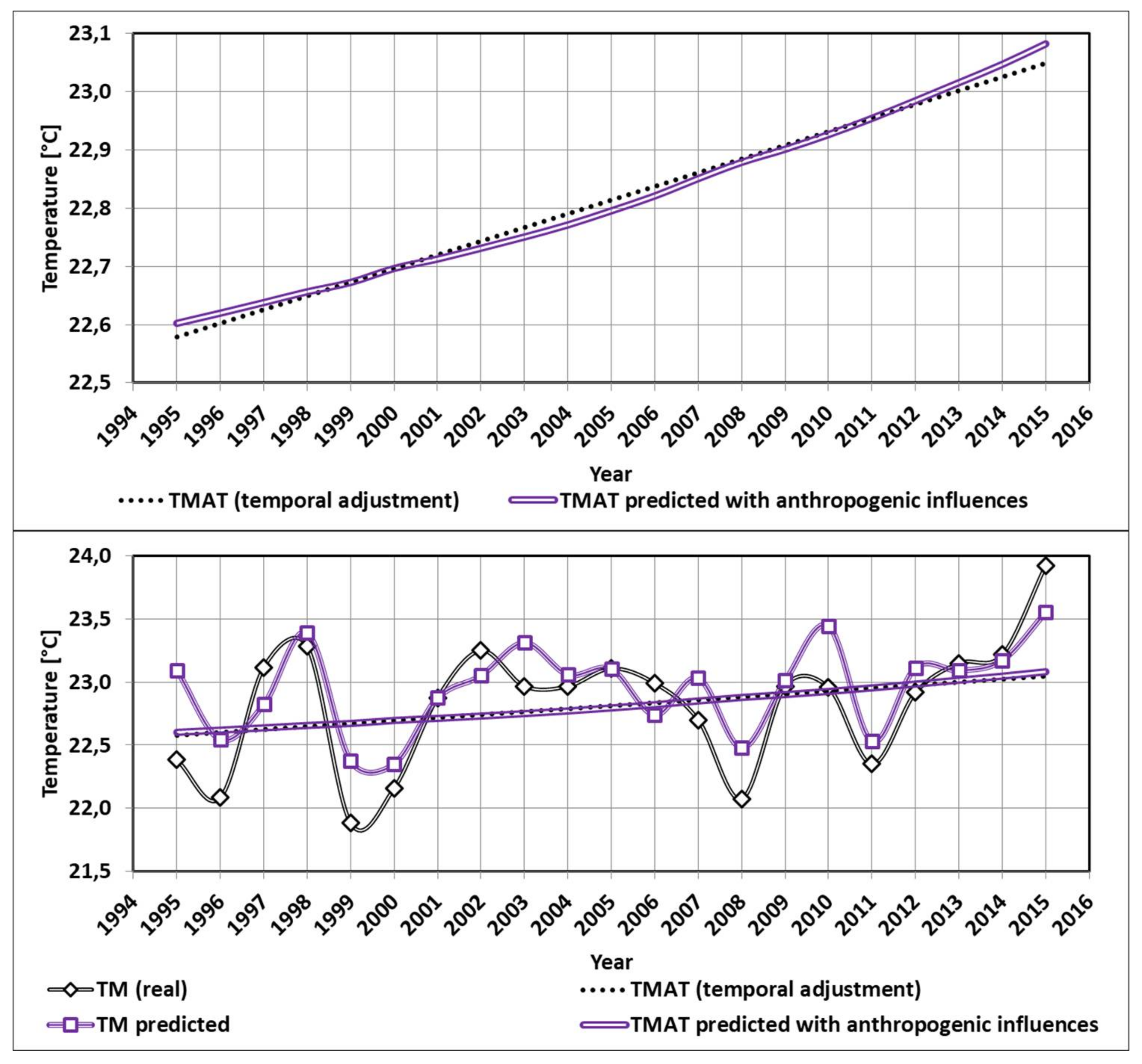
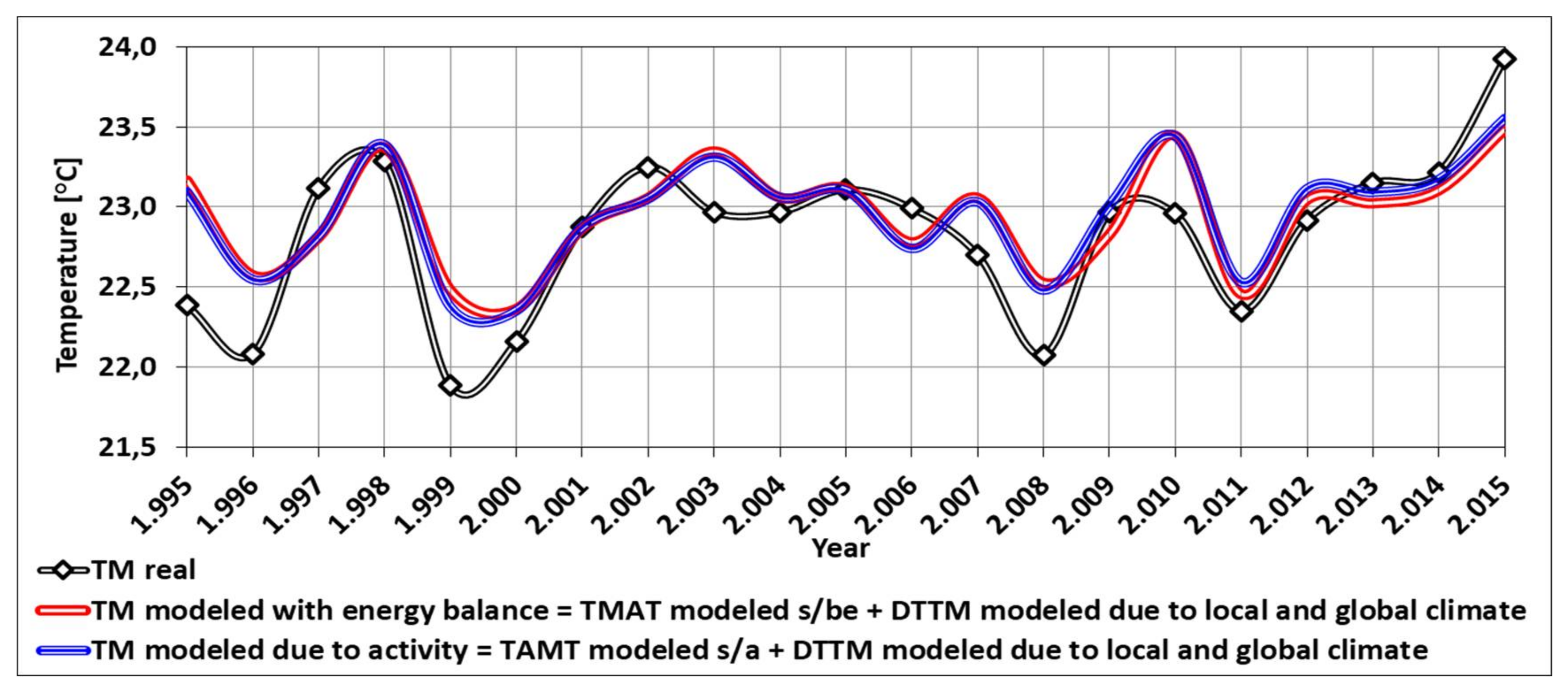
Figure 15 shows the modeling of DTAM temperatures and TM temperatures. To obtain modeled TM, the TBAT value, the DTSNM value and the result of modeling global and climatic changes for TM are added to modeled DTAM (see Equations (1) and (2)).
3.3. Model Based on Energy Balances
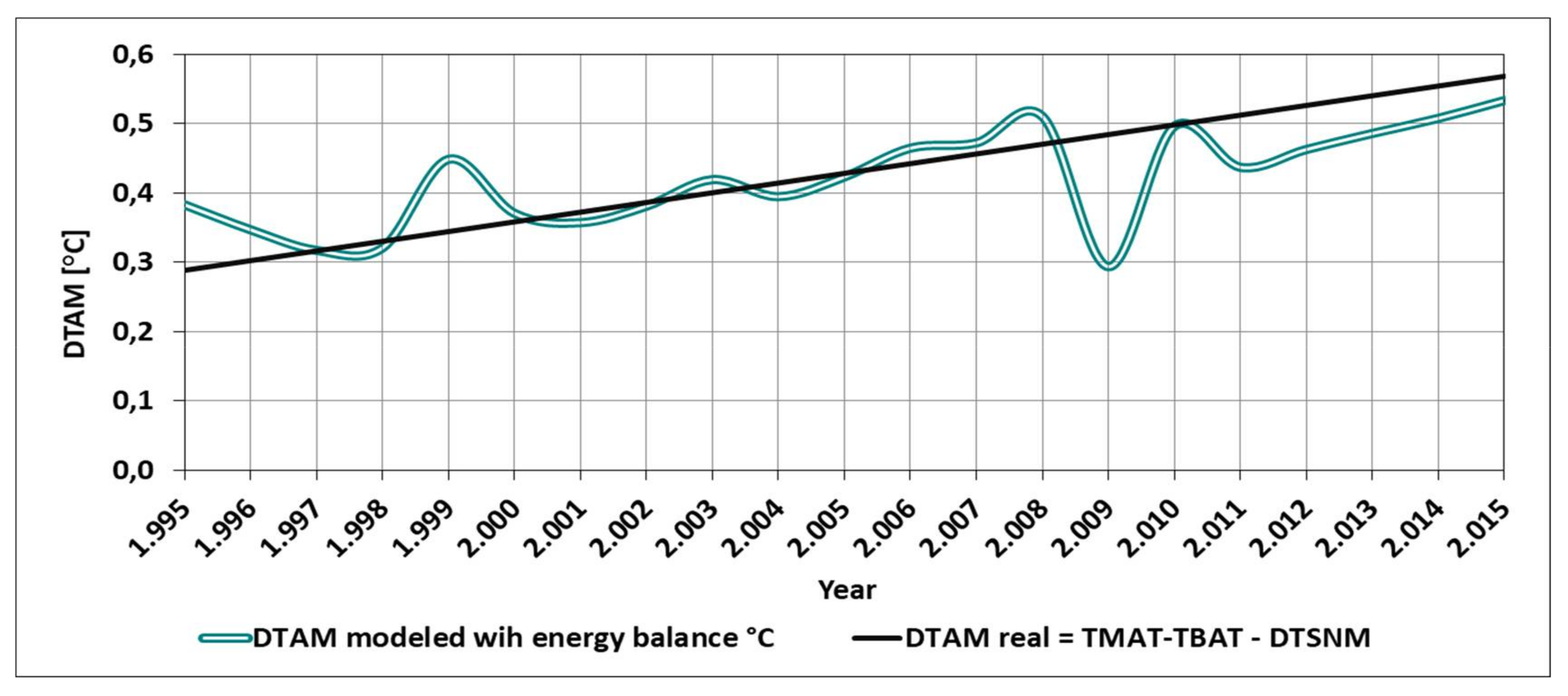
Figure 16 shows the result of modeling DTAM and its comparison with the actual value of DTAM. It is observed that the resulting model is non-linear.
4. Conclusions
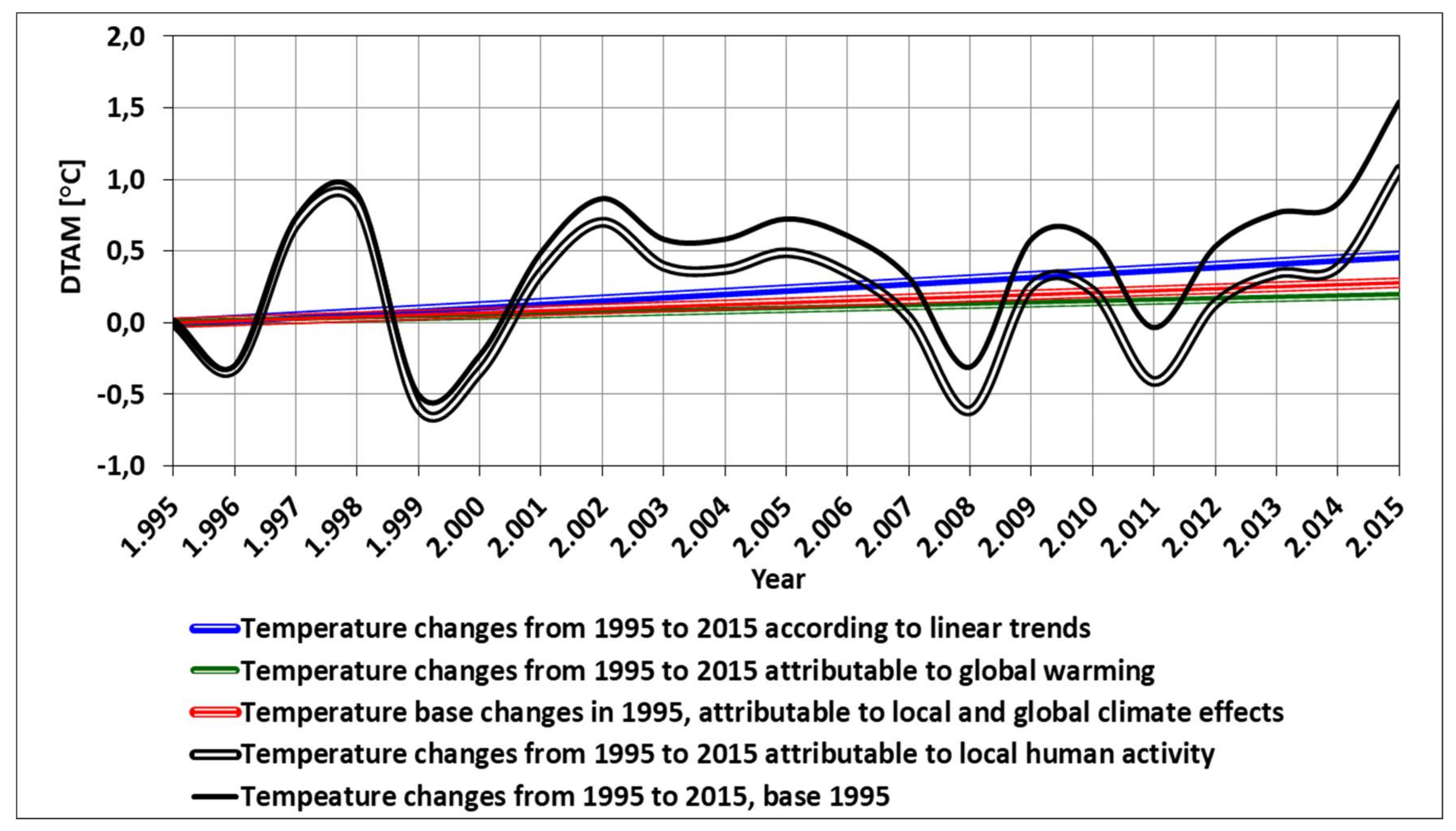
Figure 18 shows, as a summary, how the temperature change accumulates over time in the studied period of 20 years, according to the interpretations that are presented in this study.
In short, increases in mean temperature based on linear trends were found, they were estimated at 0.47 °C in the 20 years that were studied from 1995 to 2015, of which 60% is as a result of local activity and 40% due to impact of global warming. This is shown in
Table 11; however, it is a complex behavior that shows increases and decreases and is not uniform in the three stations studied.
In the results of the influence of the influence factors, it is observed that with the factors found and the values of the considered variables, a good approximation to the temperature adjustment due to the human activities is obtained. This represents a tool to estimate the temperature in the future considering the projections of the values of the variables.
Once it is taken into account, which are the most influential factors, the influence of the daily activities of citizens on the increase of temperature can be analyzed. It is observed that the total number of living beings is the most important influence and it is related to population growth, that in the case of the Metropolitan Area, has been very influenced by the arrival of population from other parts of the Antioquia department (state) and other parts of the country, all due to best health services, employment, and education opportunities in the area [
37]. This situation can be mitigated or moderated by designing policies to improve the quality of life in rural areas, thus reducing the population exodus to the cities.
From the variables that have influence on the temperature, it is clear that everyone can act in some way to influence in a positive way that the climate and temperature of the city keep evolving. For example, the use of facades and green ceilings can be promoted, with the presence of plant species or surfaces painted in fresher colors that diminish the absorption of the incoming radiation. Also, and very important, of course, the heat emission can be reduced. In the case of plants, the radiation they absorb influences evapotranspiration processes, releasing water vapor, which helps to cool the surrounding air [
38]. Another consequence is that keeping the buildings cooler, the energy consumption of air conditioners and the release of heat related to them is reduced.
The results of the energy balance allow concluding that considering the environment of the metropolitan area as a control volume, despite the simplifications, gives good results. This model seeks to calculate the temperature changes due human activity based on energy variables, which can be a useful tool for future predictions, as well as to identify the causes and propose local mitigation actions.
In both models it can be observed the influence of energy sources, fossil fuels and the consumption of electricity, make significant contributions. If energy consumption is reduced by means of energy saving actions, optimization, and a stimulation of mass public transportation is promoted, a reduction of consumption of these sources will be real, and thus the increment of the temperature will be reduced.
It is observed that in general the situation of temperature increments is due to the living habits of the population. If these become more sustainable, they will be effectively contributing to mitigating these increments.
Despite the study being strictly linked to local and specific conditions, the applied methodology can be of interest in other contexts and the correlation between different factors coming from different sectors and sources is clearly of wider interest, especially when a comparison between local and global phenomena is investigated.
5. Recommendations
With this study, it was possible to better understand the energy state of the city and the importance of monitoring various variables such as those proposed here, in order to understand climatic and environmental variations; not only can it lead to greater awareness and greater knowledge, but also to propose appropriate solutions to their reality.
The study also makes possible to see the importance of implementing a greater number of stations for measuring climate phenomena, especially temperatures, wind speeds, and mixing heights, with the goal of having long-term data to see the progress in time and the consequences of the taken actions.
The authors propose the creation of an automated system to obtain the data and the creation of indicators, such as a warming index that will allow for the public to know the actual increase in temperature due to urban or meteorological causes. Also, more attention should be given in the region to systematize the gathering of activity data of the kind used in the study. Although, given the fact that this was a first study for this region and several approximations were assumed to be able to fulfill the objectives of the study, clearly there is a real potential to use this type of modeling, so having available better data, replicating the methodology, and so refining the process, will lead to applicable conclusions and to generate and sustain public policies.
It was noted that there is an effective warm-up in the city that everyone feels, but it is also true that through initiatives, such as saving energy and fuel, everyone can help to reduce it. In the metropolitan area, there are avoidable and unavoidable energy consumptions, where for the first there is nothing more to rationalize the activity, and for the second, where the activity continues but technological updates are made to reduce the heat emissions, either by a post-process conditioning or decreasing energy consumption.
Activities are every day actions that originated in culture and ways of living, but their consequences, in the context treated in this work, are appealing to every inhabitant and every institution. They impact on everyday life in urban environment. This must be understood and applied to the daily life and the design of urban city. Not only in general terms, but in specific ways, such as establishing limits in total energy to avoid given city’s thresholds, establishing goals to increase areas of green roofs in the coming years, establishing goals on motor vehicle and industrial process efficiencies. The type of predictions that these models permit could be used to establish goals like these ones.
As an additional consideration, it can be pointed that the behavior of energy related phenomena in a large urban conglomerate enclosed by a valley is complicated, comprising many variables. Although the authors simplified the modeling of the temperature changes, it could be said that the potential understanding of the outcomes may suffer due to the still large number of variables and interrelations considered. But, one of our main goals is to attract more attention towards correlated phenomena and this study is a first step at local level. We believe the resulting increase in awareness concerning interrelated phenomena is a valuable result in itself.
Finally, it is recognized that living in a city has great advantages, such as the availability of resources and services, but at the same time the concentration of human activities brings problems that rural places do not have, which creates a certain contradiction between the enormous appeal of cities and the need to stimulate development in less populated areas, in pursuit of rationalizing and finding solutions to reduce the impact of human activity.


