1. Introduction
The rainfall pattern and amount at a certain location are important parameters affecting various natural and socio-economic systems e.g., flood protection, water resources management, agriculture and forestry and tourism. Extreme precipitation events are one of the primary natural causes of flooding. The ability to anticipate extremes of rainfall would aid in improved flood planning. Frequency analysis is used to determine the probability of occurrence of events. One goal of frequency analysis is to relate the magnitude of extreme events to their frequency of occurrence by using probability distributions.
Statistical theory for extremes is used to express that the frequency of such events is relatively more dependent on any changes in the variability (more generally, the scale parameter) than on the mean (more generally, the location parameter) of the climate [
1]. Rainfall patterns vary from country to country as well as from weather station to station. However, homogeneity can also be found. Taking annual extreme precipitation as the extreme event, Khudri et al. [
2] found that in Bangladesh, the generalized extreme value and generalized gamma four parameter distributions provide the best fit for 50% of the stations in the survey, while no other distribution was found consistently suitable for the other stations. Mandal & Choudhury [
3] studied the annual, seasonal and monthly maximum daily rainfall data for Sagar Island, located on the continental shelf of the Bay of Bengal—which is near our study area—and found that normal (N) distributions were fitted best to annual, post-monsoon and summer seasons, while Lognormal (LN2), Weibull (W2) and Pearson type 5 were fitted best to pre-monsoon, monsoon and winter seasons respectively.
Kumar [
4] and Singh [
5] found that the LN2 distribution is the best-fit probability distribution for annual maximum daily rainfall in India. Amin et al. [
6] used annual maximum rainfall based on a daily sample and found that the log-Pearson type 3 (LP3) distribution was the best-fit distribution in the northern regions of Pakistan. Eslamian et al. [
7] used the maximum monthly rainfall as an extreme event and found that in Iran, the generalized extreme value (GEV) and Pearson type 3 (P3) distributions provided the best fit. Bhakar et al. [
8] found that for monthly maximum rainfall, the Gumbel (GUM) distribution was the best fit in India.
Lee [
9] showed that LP3 distributions fitted best to 50% of the stations for the rainfall distribution of the Chia-Nan plain area of Taiwan. Ogunlela [
10] described that the LP3 provided the best fit to peak daily precipitation in Nigeria. Kwaku et al. [
11] found that the LN2 distribution was the best-fit probability distribution for one to five consecutive days’ maximum rainfall for Accra, Ghana. Olofintoye et al. [
12] showed that for peak daily rainfall in Nigeria, 50% of stations follow LP3 distributions and 40% follow Pearson type 3 (P3) distributions. Sen et al. [
13] found that the gamma probability distribution provided the best fit to monthly maxima rainfall in arid regions in Libya. Arora & Singh [
14] found that the LP3 distribution recommended by the U.S. Water Resources Council (USWRC) in 1967 was the best method of flood frequency analysis in the United States.
The frequency of extreme events such as precipitation and floods can be expressed in terms of the “return period,” also known as the “recurrence interval.” In extreme value analysis, the return period is defined as the average length of time between events of the same magnitude or greater. It is derived from quantiles of a parametric probability distribution fitted to the extreme values of the recorded data [
15]. A goal of the frequency analysis of extreme events is to estimate the value of the event magnitude corresponding to a given return period i.e., the maximum daily rainfall that can be expected to occur every 50 years.
Bangladesh is an agriculture based economy where the role of precipitation is important. The extreme events of rainfall may affect agriculture, ecosystems, biodiversities and livelihood patterns. It is important to extract the patterns of extreme rainfall events to determine risk factors which can be used to develop long-term measures to save lives and property. In the short term, precipitation plays an important role in flooding every year.
The present work focuses on two important issues. First, to find the best-fit models for determining the frequency of extreme rainfall events in Bangladesh. Second, to extract expected maximum monthly rainfall over return periods of 10, 25, 50 and 100 years. These can be used to develop plans and policies for reducing risk and damage from extreme rainfall events in both short and long-term planning.
2. Data and Study Area
Bangladesh is mainly a riverine country. 79% of the land is occupied by the delta plain, 12% is occupied by the Chittagong hill tracks located in the southeast and northeast part of the country and 9% is occupied by four uplifted blocks which are mainly situated in the northwest and central part. Almost the entire land is floodplains except the south-eastern and north-eastern hilly areas. The Bay of Bengal is situated at the south, being a source of water vapour that passes over the country and contributes to increased rainfall. During the monsoon period, excessive rainfall occurs. Rivers which originate from the Himalayas at the north flow through Bangladesh and often cause flooding during this time. The highest elevation in the delta plain is 105 m above sea level, which is found in the northern area. Elevations decrease in the coastal south. In the Chittagong hill tracks in the southeast altitudes vary from 600 to 900 m above sea level.
The climate of Bangladesh is characterized as a tropical monsoon climate [
16]. From June to October heavy seasonal rainfall occurs. About 72% of all rainfall occurs during the summer and monsoon period [
17].
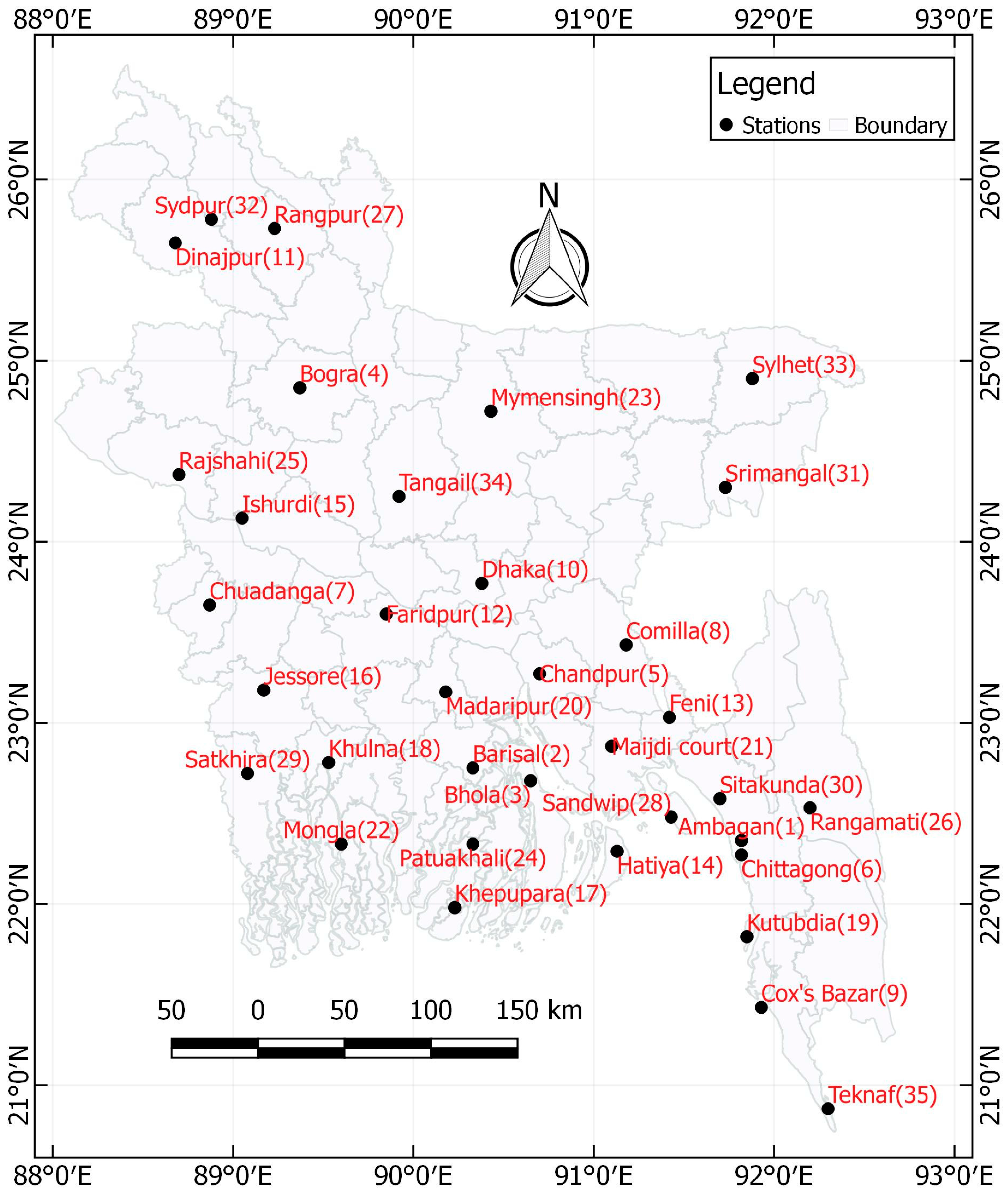
Time series of rainfall records were collected from the Bangladesh Meteorological Department (BMD) for 35 different locations all over the country (
Figure 1). The data was provided as the daily total rainfall in millimetres. This analysis uses 30 years of data from 1984–2013. However, there are 6 stations (Ambagan (15 years), Chuadanga (25 years), Mongla (23 years), Kutubdia (29 years), Sydpur (23 years), Tangail (27 years)) which did not have 30 years of available data. The total rainfall of each calendar month was calculated. Then the calendar month in each year with the highest total was taken as the maximum monthly rainfall. This yields 30 maxima (1 for each year) for each station (with the exception of the previously noted six stations). This maximum monthly rainfall is used as the parameter for analysis of extreme rainfall estimation. The maximum monthly rainfall for the entire country always occurs in the monsoon period of June to October. At individual stations, the maximum monthly rainfall occurs in July, August or September in all of the 30 years studied. The best-fit probability distributions of these meteorological locations in Bangladesh are determined.
3. Methodology
For selecting the best-fit probability distribution for a certain location, the choice of probability distribution models is important. In this section, the selected distribution models which are commonly used in extreme rainfall analyses are presented. The method of parameter estimation, the goodness of fit tests for model selection, both numerical and graphical and the return period estimation procedure are presented.
3.1. Commonly Used Probability Distributions
This analysis adopts commonly used frequency distributions used in previous studies. The method of moments (MOM) estimators are used for parameter estimation of the distributions. They are often simple to derive but when MOM estimators are either too awkward or unavailable, the
L-moments are used to estimate the parameters of the selected distributions. The
L-moments are more robust than conventional moments. One disadvantage of the
L-moment ratios for estimation is their smaller sensitivity. For calculating the parameters by using MOM; the sample mean
, standard deviation
σ and coefficient of skewness
γ are determined by the following equations:
where
n is the number of observations in the data set,
i is the observation number and
Xi is the observation data.
The following distributions with the method of parameter estimation are used in our study. Note that the variable X represents observed data, while x represents any possible value of that data and is used as the basis to create the continuous distribution functions below. Fx(x) is the value of the distribution function for the point where x corresponds to an observed data value of X.
3.1.1. Normal
The Gaussian or N distribution is often applied in annual precipitation and runoff analysis [
18]. The two moments, mean
μ and variance
σ2, are the parameters of the normal distribution. The probability density function (pdf),
f(
x) and cumulative distribution function (cdf),
F(
x) for a normal random variable
x are expressed as,
for the range of −∞ <
x < ∞. The symmetric nature of the N distribution should tend to make it less suitable for fitting to heavy-tailed data, like some of the rainfall data samples of this study.
3.1.2. Log-Normal
The pdf and cdf of the 2-parameter Log-normal (LN2) are expressed as:
where the range of random variable is
x > 0. The logarithm of the
x variable,
y =
ln(
x), is well-described by a normal distribution. By using MOM estimators, the two parameters are expressed as follows:
which are the commonly used parameters of the LN2 distribution. Here,
σY is the standard deviation and
μY is the mean for the LN2 distribution. The LN2 should be better suited than the simple N distribution as it allows for a “heavy tail” on one side, which can better fit extreme rainfall data.
3.1.3. Pearson Type 3
One of the most commonly used distributions in hydrology is the P3 distribution which is a two-parameter Gamma distribution with a third parameter for the location. The pdf and cdf of P3 are:
The parameters are shape
β, scale
α and location
ξ which are estimated by MOM estimators, which are:
3.1.4. Log-Pearson Type 3
The LP3, another gamma family distribution, describes a random variable whose logarithm follows the P3 distribution. The pdf and cdf of LP3 are as follows:
3.1.5. Exponential
The exponential distribution (EXP) is a special case of the Gamma family characterized by skewness. The pdf and cdf are:
with a range of
ξ ≤
x < ∞. The location,
ξ and shape parameters, α, of the EXP distribution are estimated by
L-moment estimators and expressed as:
where
λ1 is the
L-location or mean and
λ2 is the
L-scale of the distribution (for more details see [
19]).
3.1.6. Gumbel
The extreme value type 1 distribution, also called the GUM distribution, is often used to represent a maximum process, for example the maximum rainfall or flood discharge or the lowest stream flow or pollutant concentration. The GUM distribution is used in Finland and Spain as the best-fit distribution for flood data [
20]. The pdf and cdf:
where
α is the scale parameter and
β is the location parameter for the GUM distribution. We can calculate the parameters by any of the estimators easily. Here, the MOM was used to estimate the parameters.
3.1.7. Generalized Extreme Value
A well-known three-parameter distribution for maxima is the GEV. In many European countries, such as Austria, Germany, Italy and Spain, the GEV distribution is recommended to provide the best-fit to flood data [
20]. It includes a shape,
κ, a scale,
α and a location,
ξ, parameter. The parameters are estimated by
L-moment estimators. The pdf and cdf are expressed as:
with a range of
where
τ3 is the
L-skewness of the distribution [
19].
3.1.8. Weibull
The extreme value type 3 distribution or W2 is often used for minimum stream flows and related fields. As this is an analysis of maximum rainfall it is expected that the W2 will not be as suitable as other distributions. Stendinger et al. [
21] listed the W2 as a commonly used frequency distribution in hydrology. The pdf and cdf are:
with the range of
x > 0;
α,
k > 0. We estimate the parameters using the MOM estimators.
where
α is the scale parameter and
β is the shape parameter for the W2 distribution.
3.1.9. Generalized Pareto
The Generalized Pareto distribution (GP) is applied in precipitation analysis. It is useful for describing events which exceed a specified lower bound, such as rainfall events above a given threshold. The three-parameters are location
ξ, scale
α and shape
k. The parameters are estimated by
L-moment estimators. The pdf and cdf are:
with a range of
3.2. Goodness-of-Fit Test
Goodness-of-fit test statistics are used for checking the validity of a specified or assumed probability distribution model. Three procedures are used for checking the normality: graphical methods (histograms, boxplots and Quantile-Quantile plots (Q-Q plots)), numerical methods (skewness and kurtosis indices) and formal normality tests. There are dozens of tests of normality existing in statistical testing procedures. Among these, Empirical Distribution Function (EDF) tests provide a measure of the discrepancy between the empirical and theoretical distributions [
22]. The most well-known EDF tests are the Kolmogorov-Smirnov (K-S) test, the Anderson-Darling (A-D) and the Cramer Von Mises test [
23,
24]. The K-S and the A-D tests were applied here. As a graphical test, a Q-Q plot was applied. Also, the root mean square error (RMSE) was used to test the best model. A graphical test was also applied to compare the observed and estimated values.
3.2.1. Kolmogorov-Smirnov (K-S) Test
The K-S test statistic, the
supreme class of EDF statistics, is based on the maximum vertical difference between the theoretical and empirical distributions [
25]. The main goal of this test is to compare the empirical cumulative frequency (
Sn(
x)) with the cdf of an assumed theoretical distribution (
FX(
x)). The maximum difference between
Sn(
x) and
FX(
x) is the K-S test statistic. For a sample size
n, the data is rearranged in increasing order,
X1 <
X2 < … <
Xn and the K-S statistic is assessed for each ordered value:
where
is the critical value,
α is the significance level and
k is the rank order of the data set.
3.2.2. Anderson-Darling (A-D) Test
The A-D test, the most powerful EDF test, was first introduced by Anderson & Darling [
26] to place more weight at the tails of the distribution [
27]. In cases with relatively large extremes, it may be expected the A-D test to be more suitable to select the best-fitted model to data maxima. The A-D test statistic, the
quadratic class of the EDF test statistic, is expressed as
A2 as follows:
where
Fx(
xi) is the cdf of the proposed distribution at
xi, for
i = 1, 2, …,
n. The observed data must be arranged in increasing order, as
x1 <
x2 < … <
xn.
In the K-S test, both the theoretical and empirical cdfs are relatively flat at the tails of the probability distributions. On the other hand, the A-D test gives more weight to the tails. This can be a more accurate test when the tails of the selected theoretical distribution are the focus of the analysis, as with extreme rainfall.
3.2.3. Root Mean Square Error (RMSE)
The smallest RMSE value indicates the best-fit model of the variate and gives the standard deviation of the model prediction error. It measures the differences between observed and estimated values. The RMSE can be expressed as the following equation:
where
xi denotes the estimated value and
X denotes the observed value. The RMSE gives a relatively larger weight to large errors by squaring them.
3.2.4. Graphical Test
A graphical test is one of the most simple and powerful techniques for selecting the best-fit model. Here the Q-Q plot of observed and estimated values is presented. To calculate the plotting position of the non-exceedance probability
pi:n various plotting position formulas are used for the specific distributions. Most of the plotting position formulae currently in use have the following form:
where
n is the rank of the observed value
X (
X(i) is ascending order),
n = 1, 2, 3, …,
N.
N is the total number of observed values and
a is a constant.
Blom’s plotting position (
a = 3/8), which gives unbiased quantiles, is used here for N, LN2, P3, LP3 distributions; Gringorten’s plotting position (
a = 0.44) is used for EXP, GUM, W2, GP distributions; Cunnane’s plotting position (
a = 0.4) is used for GEV [
21,
28,
29]. To construct the Q-Q plot the observed data,
X(i), versus the estimated values,
x(
F), are plotted, where
x(
F) is the quantile function, with
F determined by the
pi:n for the certain probability distribution.
3.3. Return Period
One of the important objectives of frequency analysis is to calculate the recurrence interval or return period. If the variable (
x) equal to or greater than an event of magnitude
xT, occurs once in
T years, then the probability of occurrence
P(
X ≥
x) in a given year of the variable is:
The precipitation amounts associated with the 50- or 100-year average return periods cannot be directly estimated from a data set but must be extracted from the 98th and 99th percentiles, respectively, of a fitted distribution (i.e., [1–0.98
-year]
−1 = 50 years and [1–0.99
-year]
−1 =100 years) [
15].
4. Results and Discussion
The main goal of this paper is to identify the best-fit probability distribution for every station which yields the maximum monthly rainfall for return periods of 10, 25, 50 and 100 years. These estimates can provide useful guidance for policy making and decision purposes. Knowing the return period of extreme and catastrophic events can be used in determining the risk level of damage by extreme events e.g., rainfall, floods etc.
4.1. Selecting the Best-Fit Results
The compiled data in our study showed the rainfall range varied widely in all the stations. The site’s geographical location e.g., longitude, latitude, elevation and the surrounding environmental factors are among the reasons for the variation of rainfall. The south-eastern part of Bangladesh has the highest amount of measured precipitation e.g., Sandwip station has recorded a high of 3001 mm monthly maximum rainfall over the past 35 years. On the other hand, the stations in the region of the north-western part of Bangladesh measured the lowest amount of precipitation (such as Ishardi station, with a 664 mm monthly maximum) compared to the other regions.
Table 1 shows the station names, statistical summary results, the best-fit results of K-S, A-D, RMSE and the best-scored results. The best-fit result is taken as the smallest goodness-of-fit result among all probability distributions developed for each station. The table shows the test statistic result of the best-fit distribution type in probabilities for each model selection tool (K-S, A-D, RMSE). All developed probability distributions are ranked with each selection tool (rank 1 is the best-fit). The 3 ranking results are summed to yield a ranking score. The distribution model of each station with the smallest ranking score is selected as the best-fit distribution model.
The Q-Q plots of all stations were created and the distribution fit with observed data was found using the RMSE. As an example, the plots for station Dinajpur are illustrated in
Figure 2. The main purpose of the probability distribution fitting here is to most accurately represent the low probability, extreme events on the extreme right tail. By using a Q-Q plot the level of fit on the extreme right tail can be studied [
30]. Any perfect matches with observed data points would fall on the [1:1] line. In
Figure 2, the GEV distribution matches the data well, with the right tail falling near the [1:1] line. In the case of all other stations there is no common representation pattern of all the distributions. The right tail was often over-estimated or under-estimated. For most of the stations, the GEV, P3, or LP3 distributions perform better in representing the right tail. However, to select the best fit probability model not only the graphical observation but the numerical test is also important.
The result of statistical parameters, mean, standard deviation and coefficient of skewness of all stations are included in
Table 1. Stations at Hatiya and Sydpur show negative skewness. With distributions tending to have a heavy tail on the right side (in this case more extreme rainfall) the skewness will be positive and relatively high. The absolute value of the skewness reveals the relative magnitude of the deviations from the mean. The coefficients of skewness of 12 stations are greater than 1, thus can be regarded as highly skewed. Eight stations lie within the range of 0.5 to 1, thus are moderately skewed. Fifteen stations are approximately symmetric, lying within the range of −0.5 to 0.5.
The best-fit test statistic results of K-S, A-D and RMSE are tabulated in
Table 1. Among all the stations, it was found that among all distributions, the GEV yielded the most cases of best-fit distributions, while the P3 and LP3 yielded the second and third amount of best-fits respectively. There were no best-fit results from the EXP distribution. The LN2, GUM, GP distributions gave some best fit results among all stations. The other two distributions, W2 and N gave only a few best fit results. The trend of weak fitting of the two-parameter distributions (W2, N, EXP) can be expected as they are less flexible than three-parameter distributions (GEV, P3, LP3). The GP was not among the best performing distributions although it has three-parameters but this distribution is commonly used with peaks over threshold of precipitation or flood values. The weak fit of the W2 is expected as it is often used for minima estimation. However, most stations were best fitted by the GEV, P3 and LP3, all of which have three parameters.
In most of the cases the three goodness of fit tests yielded different types of distribution. To conclude, for selecting the best-fit distribution for every station a ranking system was made, with rank 1 being the best, 2 the second best and so on. The distribution type with the lowest sum of the three rankings is selected as the best fit distribution for each of the stations. Four stations had two distributions with the same value of best score result (a tie between two types). In the best score result, 36% stations are best-fitted by the GEV distribution. Each of the P3 and LP3 yielded the best-fit in 26% of the stations.
4.2. Return Period Results
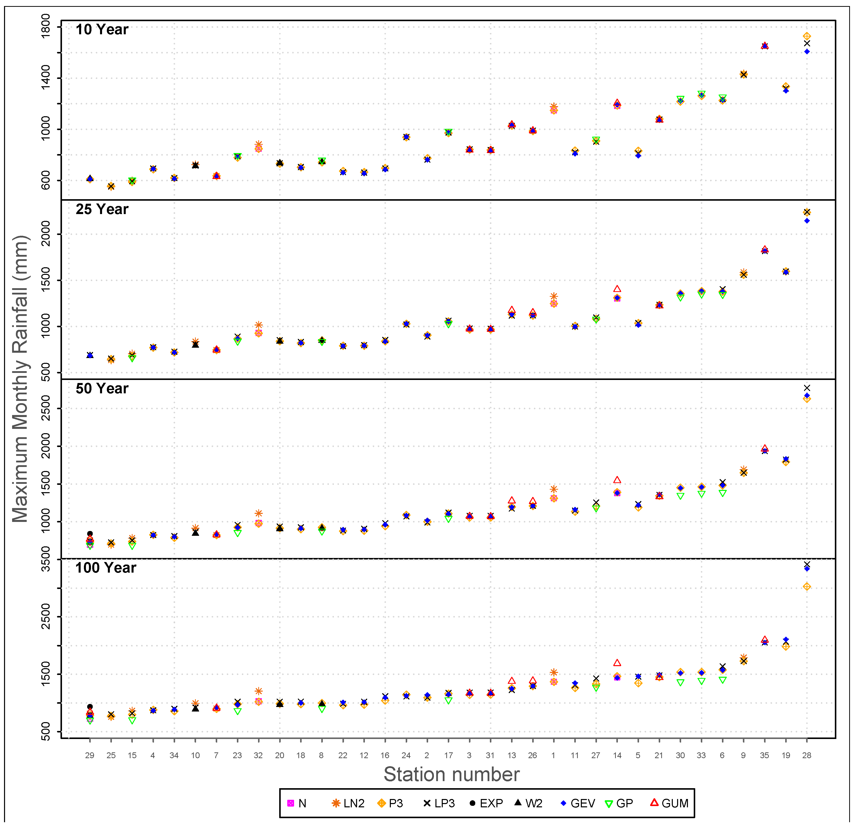
In
Figure 3, 10-year, 25-year, 50-year and 100-year rainfall return levels of all stations are illustrated. The horizontal axis, ranging from 1 to 35, represents the station numbers which are given in
Table 1. The vertical axis represents the maximum monthly rainfall. There are four parts in this figure. Return periods of 10 years, 25 years, 50 years and 100 years are represented vertically from top to bottom. The return levels of the best-fit distributions for each station are shown here. As an example, for the station Dinajpur, station number 11, which is best-fitted by the GEV distribution, the rainfall amounts of 10, 25, 50 and 100 year return periods are 809 mm, 997 mm, 1161 mm and 1347 mm respectively.
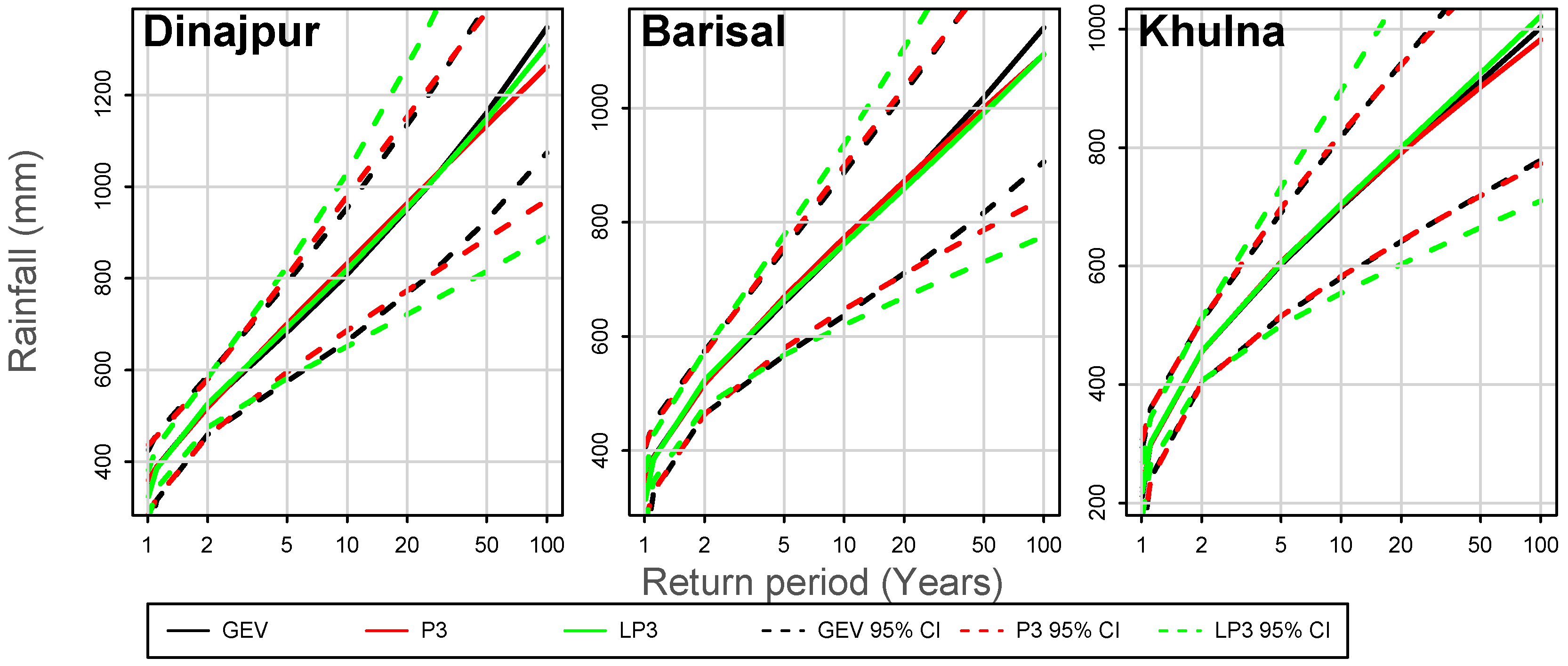
The confidence interval, a statistical estimate of the range given a chosen level of probability within which a true value can be expected to fall, is essential in risk analysis as well as in the design process. The upper and lower boundary values of the confidence interval are called confidence limits. In
Figure 4, the rainfall return levels of 1 to 100 years with 95% confidence intervals are illustrated for 3 stations. Here, the sample data size is relatively small compared to the return levels. Anticipating up to 100-year return periods with only 30 years of data available unavoidably yields much lower confidence in the results as the return period increases. It is apparent for these cases that the GEV tends to yield the narrowest range of 95% confidence with the P3 nearly as good, while the LP3 yields a much wider range. If the sample size is small the confidence interval is quite wide. As the sample size increases, that is, as more weather data is recorded over time, the width of the confidence interval around the estimated rainfall magnitude will likely be reduced as improved distributions are found.
In the south-eastern region, for example near the area of the station name Kutubdia, Cittagong, Cox’s Bazar, Teknaf, more intense rainfall occurred than in the other regions. During the monsoon time landslides occur frequently in this area causing deaths and damage of assets. Extreme amounts of rainfall in the piedmont of hilly areas is the main source of flash floods. Landslides often occur in the areas composed of unconsolidated rocks [
31]. The Daily Star, the leading daily newspaper, reported on 13 June 2017 that a landslide in the hilly area caused 133 deaths [
32]. Sarker & Rashed [
31] also mentioned that slope saturation by water is the main cause of landslides. Saturation occurs due to excessive rainfall.
The information of return periods can help guide policy makers and planners. They can more easily make their decisions for a given span of time using the expected maximum monthly rainfall as determined by the return period. Taking the example of Barisal as shown in
Figure 4, a risk level plan using the GEV distribution for a 50-year span would anticipate that the expected maximum monthly rainfall is 1018 mm on average, with a 95% confidence that it will range from 816 mm to 1220 mm. This can then be used to develop more detailed risk and damage estimates (i.e., flooding levels, infrastructure damage etc.).
5. Conclusions
The rainfall patterns vary across all locations. The site’s geographical location and surrounding environment are important factors in the variation of the rainfall pattern. The south-eastern part measures the highest amount of precipitation while the north-western part has the lowest amount of rainfall.
In terms of selecting the best-fit distribution to model the maximum monthly rainfall for a certain location, the result varied significantly. Parameters of the distributions were estimated by the method of moments and L-moments estimators. The fit results were calculated by the K-S, A-D and RMSE as well as a graphical procedure, the Q-Q plot. The return period, which is important in determining long-term risks, was also calculated.
In some cases, all three test statistics yielded the same best-fit distribution type. However, for most of the locations the testing statistics yielded different best-fit distribution types. Thus, a scoring system was used to determine the best fit distribution for each location. The best-fit result of each station was taken as the distribution with the lowest sum of the rank scores from each test statistic. GEV, P3 and LP3 showed the larger number of best-fit results compared to other distributions. In the best score results, GEV fitted 36% of the stations, while P3 and LP3 each fitted 26% of the stations. This result aligns well with results in the literature. The GEV was also the most common best fit in the research by Khudri et al. [
2] on annual extreme values of precipitation in Bangladesh. Also, the GEV and P3 were the most common best fits for maximum monthly rainfall in Iran as found by Eslamin et al. [
7].
The more practical result of this paper was the return period calculation for all locations and all distributions. The presentation of all distributions gives a clear inspection of the range of projected return periods, including the best fit (most likely) result. Here, 10-year, 25-year, 50-year and 100-year return periods of rainfall return levels were illustrated. A policy maker making a risk analysis for a 50 year plan could use the 50 year return period result of projected maximum monthly rainfall to determine flooding risks, damage projections, etc. The 100 year return period results are high intensity but low probability which has an inverse relationship with 10 year return period results. It depends on the policy makers to choose the duration and risk level.
The results of this study can be used to develop better models of risk and damage from extreme rainfall events and flooding. These estimates can help policy makers to create initiatives with the result of saving lives and property. In addition, Knowledge of the pattern of extreme rainfall will be useful in various disciplines such as the environment, agriculture, construction and building structures.


