Article

An Exposure-Mortality Relationship for Residential Indoor PM2.5 Exposure from Outdoor Sources

1
Department of Social & Environmental Health Research, London School of Hygiene & Tropical Medicine, 15–17 Tavistock Place, London WC1H 9SH, UK
2
UCL Institute for Environmental Design & Engineering, University College London, Central House, 14 Upper Woburn Place, London WC1H 0NN, UK
3
School of Energy & Environment, City University of Hong Kong, Yeung Kin Man Academic Building (AC1), Tat Chee Avenue, Kowloon, Hong Kong
4
Institute of Occupational Medicine, Research Avenue North, Riccarton, Edinburgh EH14 4AP, UK
*
Author to whom correspondence should be addressed.
Climate 2017, 5(3), 66; https://doi.org/10.3390/cli5030066
Submission received: 29 June 2017 / Revised: 18 August 2017 / Accepted: 24 August 2017 / Published: 26 August 2017
(This article belongs to the Special Issue Urban Climate, Air Pollution, and Public Health)

Abstract

:
A large proportion of particulate air pollution exposure in urban areas occurs due to the penetration of outdoor pollution into the residential indoor environment. Theoretical considerations suggest that quantifying health effects due to changes to indoor particulate concentrations derived from outdoor sources requires the adjustment of exposure-response coefficients based on epidemiological studies of outdoor air. Using the PM2.5-mortality coefficient from the American Cancer Society (ACS) cohort study as an example, we developed a theoretical model to quantify the relationship between the published coefficient and one based on personal exposure, and explored how this adjusted coefficient might be applied to changes in indoor PM2.5 from outdoor sources. Using a probabilistic approach, our estimated average mortality coefficient for personal PM2.5 exposure is 30–50% greater than the ACS coefficient. However, since the indoor PM2.5 of outdoor origin accounts for only a proportion of the overall exposure, the average net adjustment required for indoor exposure is very modest. The results suggest that it is generally appropriate to apply unadjusted exposure-response functions derived from cohort studies to assess the health impact of changes in indoor particle concentrations from outdoor sources. However, it may be important to re-scale the coefficients for assessing exposures of population groups who spend a greater proportion of their time at home.

1. Introduction

Growing attention on reducing greenhouse gas (GHG) emissions, particularly in cities, has increased interest in housing energy efficiency and its potential health effects. Improving dwelling energy efficiency may have appreciable near-term net benefits to health from increased indoor temperatures in winter and other changes to the indoor environment [1,2], an example of the health “co-benefits” of GHG mitigation. However, there is also the potential for adverse health effects, especially if efficiency is in part achieved through tightening ventilation control; reducing ventilation reduces the exposure to pollutants originating from the outdoor air, but increases the exposure to pollutants generated inside the home [3,4,5].
Key to any analysis of a housing-related health impact is the exposure to fine particles from the outdoor air because of the well-established health effects of PM2.5 [6,7,8,9,10,11]. Changes in indoor particle levels from housing interventions are estimable from building physics models [12], but it remains unclear what exposure-response functions should be applied to those changes for calculating the health impact. The epidemiology is dominated by time-series and cohort studies that relate health outcomes to outdoor air pollution measured at one or a few fixed-site urban monitoring stations [8,13]. Theoretical considerations, which we will present in this paper, suggest that coefficients derived from such studies may not be directly applicable to changes in particle concentrations in the indoor air.
A study in Finland showed that assessing personal exposure based on outdoor fixed air quality monitoring sites overestimated exposures to outdoor sources [14] and hence, the authors concluded that exposure-response functions based on outdoor fixed-site data may underestimate the true association for personal exposures to PM2.5 of an outdoor origin. This exposure misclassification occurs because the indoor environment acts as a sink for particles (due to filtration by the building fabric and deposition on internal surfaces), so that indoor levels of outdoor-generated particles are generally lower than those in the outdoor air and the range of variation is correspondingly smaller. Thus, a 1 µg/m3 increase in PM2.5 levels in outdoor air would translate into an increase in the component of indoor PM2.5 derived from outdoor sources of less than 1 µg/m3. Based on this principle, Ji and Zhao (2015) developed a method for estimating the fraction of mortality attributable to outdoor particles that is due to exposure indoors [15]. However, the work did not explicitly develop exposure-response coefficients for application to indoor exposures and did not account for spatial variations in ambient pollution that may have a considerable impact on estimates of health impact, especially in urban areas where levels of spatial variability are greater.
In this paper, we consider whether coefficients obtained from semi-ecological cohort studies should be adjusted for assessing the long-term health impact of housing conditions which result in changes to indoor particle pollution derived from the outdoor air. To achieve this, we have developed a conceptual model to represent indoor exposures due to outdoor sources. We have parameterized the new model using evidence on parameter distributions from the literature and have used a probabilistic approach to estimate the required adjustment for indoor exposures.

2. Materials and Methods

A first consideration is the distinction between particles originating from the outdoor air and those derived from indoor sources. There is a gap in scientific evidence about the long-term health effects of exposure to particles generated inside the home. Epidemiological evidence is emerging for the high levels of particle exposure produced by the inefficient and poorly ventilated combustion of biomass in low income settings [16,17] and there is also evidence regarding the health risk due to particulate matter originating from tobacco smoke [18], but in general, there is little direct evidence that addresses the long-term effects of exposure to fine particles generated inside the home. The differences in the nature of the particles of an indoor and outdoor origin and in their potential (but largely unquantified) relative toxicity are sufficiently great as to require entirely separate consideration [19,20,21,22]. In this paper, we focus exclusively on particles penetrating the home from outside.

2.1. Theoretical Considerations

As our focus, we take the use of exposure-response coefficients for fine particles (maximum aerodynamic diameter of 2.5 microns, PM2.5) derived from cohort studies, and consider how to modify them for use in studies estimating the impact on health due to changes in levels of indoor PM2.5 derived from outdoor air. We take as our specific example the PM2.5-mortality coefficient published by the American Cancer Society (ACS) study [8] because of its pre-dominant use in health impact assessments (HIA) [7,11]. We divide our model into two parts:
  • The relationship between the PM2.5-mortality coefficient and the unit personal exposure in the ACS study.
  • The application of the ACS personal PM2.5 exposure-mortality relationship to estimated changes in residential indoor PM2.5 exposure.

2.2. A PM2.5 Coefficient for Personal Exposure

The ACS study estimated the increment in mortality associated with a unit increase in long-term average concentrations of PM2.5 measured by ambient monitors in each study city (strictly each metropolitan statistical area). It assumes that the relationship between mortality D and long-term outdoor PM2.5 concentration as monitored in each city ( C m ) is (log-) linear with no threshold, as follows:
log ( D ) = α + β C m
where α is the city-specific baseline log mortality rate due to other risk factors, and β is the ACS PM2.5-mortality coefficient (in the ACS study, the central estimate for β = 1.06).
We make three principal assumptions:
  • For each city and each dwelling in that city, the concentration of residential indoor PM2.5 derived from outdoor sources ( C a i ) is related to the concentration immediately outside the residence by a fixed ratio, irrespective of the outside concentration (i.e., C a i = F I N F C a ), where F I N F is the infiltration ratio for that dwelling and city;
  • The proportion of time that subjects spend indoors, y , is independent of the infiltration ratios F I N F ;
  • The level of outdoor pollution around the home is related to that at the measurement site ( C m ) by a time- and space-invariant ratio, r (i.e., C a = r C m ), and is representative of all concentrations to which the population are exposed outside the home (i.e., all non-residential microenvironments which will not be affected by housing modifications).
Using the notation of Table 1, based on Wilson et al. (2000) [23], the total residential indoor PM2.5 concentration in each city and dwelling is the sum of the PM2.5 of an indoor origin,   C i g , and the PM2.5 derived by an ingress of outdoor air, as follows:
C a i = F I N F C a
C i = C a i + C i g = F I N F C a + C i g
Thus, the total personal exposure, E t , is an average of the outdoor and indoor exposure weighted for the proportion of time that an individual spends outdoors, y , and indoors ( 1 y ):
E t = ( 1 y ) C i + y C a
Substituting C i in (3) and remembering that we assume that the outdoor PM2.5 concentration is representative of all exposure outside the home (unaffected by housing modifications):
E t = ( 1 y ) ( F I N F C a + C i g ) + y C a = ( 1 y ) ( F I N F r C m + C i g ) + y r C m
In deriving Equation (4), we have substituted C a with r C m . Since this expression represents a relationship between an individual’s total personal exposure and the outside level, whereas the ACS study associates mortality with a single measure of PM2.5 concentration for a city, we need to further show that the expression also holds for average E t and C a values. Principal assumption (2) implies that the average of the product of y and F I N F over all cities and dwellings is equal to the product of the averages ( X Y ¯ = X ¯ Y ¯ if X and Y are independent, where the bar denotes the averaging operator) [24]. In this case, Equation (4) is therefore valid using averages for the cities of the ACS study as a whole. Averaging both sides of Equation (4) gives:
E ¯ t = ( 1 y ¯ ) ( F ¯ I N F r ¯ C ¯ m + C ¯ i g ) + y ¯ r ¯   C ¯ m
Hence, the change in the average total personal exposure for a unit change in C ¯ m is:
d E ¯ t / d C ¯ m = r ¯ ( ( 1 y ¯ ) F ¯ I N F + y ¯ )
where the operator d denotes differentiation. At this point, having demonstrated that expression (4) is also true for average values, we shall dispense with the bar symbols. Now, we assume that health effects may be represented by:
β C m = β * E t
where β is the coefficient for the change in risk per µg/m3 PM2.5 measured at the monitor and β * is the coefficient for the change in risk per µg/m3 PM2.5 personal exposure (more precisely, these are the exponent forms). Thus, by differentiating (7) with respect to C m and equating it to the right hand side of (6), we get:
β * = β / ( r ( ( 1 y ) F I N F + y ) )
Equation (8) provides a scaling factor with which to adjust the outdoor exposure-response coefficient β to reflect the change in personal exposure.

2.3. Application to Changes in Indoor PM2.5 from Outdoor Sources

To apply this adjustment to other settings for HIA studies based on changes in indoor PM2.5, a further step is necessary to account for the contribution of the change in indoor PM2.5 to overall personal exposure. Under principal assumption (3), any housing intervention is assumed to have no effect on the exposure to PM2.5 outdoors or in other microenvironments. Hence, the change in personal exposure following a housing intervention, δ E t ,   is proportional to the change in residential indoor PM2.5 of an outdoor origin, δ C a i , with the constant of proportionality equal to the proportion of time spent indoors at home ( 1 y ) , where y is the proportion of time spent outside the home in the setting where the HIA is being performed (note that y is distinct from y , which represents the proportion of time spent indoors by the ACS population) and δ is the change operator:
δ E t = ( 1 y )   δ C a i
Hence, for a given change in residential indoor PM2.5 of an outdoor origin, the relative risk (RR) for health impact may be computed by multiplying Equation (8) by Equation (9):
R R = β / ( r ( ( 1 y ) F I N F + y ) ) × ( 1 y )   δ C a i
This, we propose, is the more appropriate equation to apply for the relative risk calculations associated with PM2.5 changes when estimating the health impact of housing interventions based on changes in indoor PM2.5 from outside sources. Note that, because ( 1 y ) will always be less than 1, the proportion of time spent outside the home will tend to reduce the change in relative risk when applied to changes in indoor concentrations.

3. Results

3.1. Parameterizing a Health Impact Calculation

The values used to parameterize Equation (10) have an appreciable bearing on the overall calculation of the health impact. We estimated plausible distributions in the US for each parameter based on published evidence (Table 2).
The average value for the ratio of average PM2.5 at the place of residence compared with at the monitoring location within the ACS study ( r ) is likely to be approximately 1 and this assumption is commonly made in the literature [31]. There is evidence to suggest that, in general, fixed site monitors will be located closer to the city centre than residential locations, and hence exhibit slightly higher average PM2.5 concentrations [32]. On the other hand, Adgate et al. (2002) [25] found that PM2.5 measurements outside dwellings in three US communities were significantly higher than central site measurements on days with paired samples. This study and others have found the distribution of outdoor measurements to be positively skewed and approximately log-normal with a high correlation between locations [33,34]. Precise estimates are doubtless possible if spatial models of air pollutants are applied to the ACS study cities. In lieu of detailed dispersion modelling, based on the evidence described above and our own analysis of the spatial variation in long-term PM2.5 levels across a city (New York), we have represented the distribution of r using a log-normal distribution with mean = 1.0 and standard deviation = 0.1 (Figure 1). However, given the uncertainties associated with this parameter, we have also tested the sensitivity of the model using a log-normal distribution with mean = 1.0 and standard deviation = 0.2 to represent a greater degree of spatial variability.
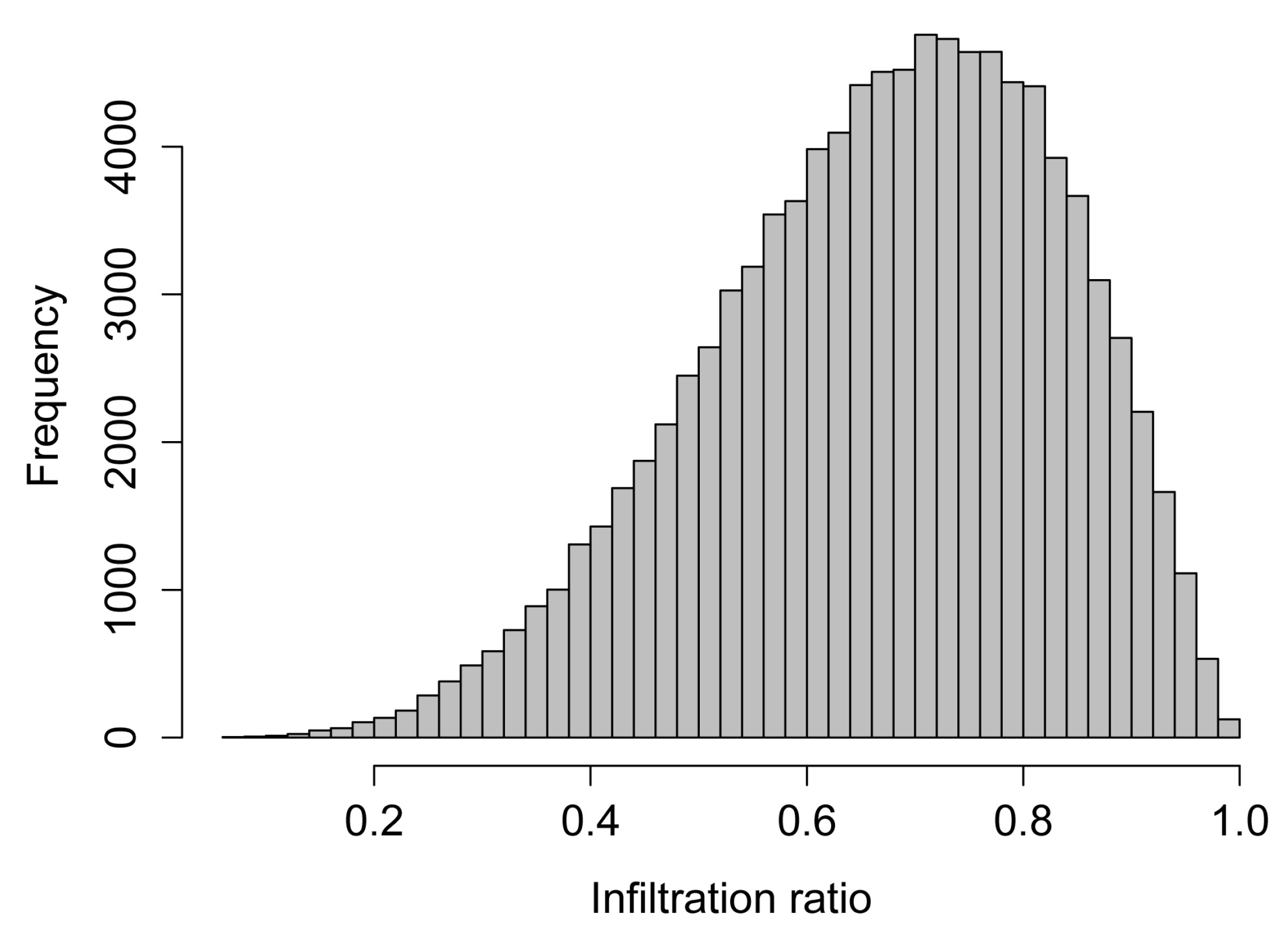
Evidence for the value of the infiltration ratio of indoor PM2.5 of an outdoor origin to outdoor PM2.5 at the home ( F INF ) is available from both modelling studies and measurements. Based on the knowledge of deposition rates and assuming a typical US air exchange value of 0.75 h−1, an average contribution to indoor fine particles due to outdoor air of approximately 65% at a steady state is likely [27]. The PTEAM study [26] estimated the actual distribution of values for this parameter in study homes using the same method and found an average of around 67% for fine particles. The values obtained during the study ranged from approximately 28% to 95% with a standard deviation of about 16%. We used these values, which are also consistent with a recent review [35], to represent F INF using a beta distribution because it is bounded between 0 and 1 (Figure 2). Our own modelling using the validated CONTAM multizone modelling software [36], suggests values in the range of 0.5–0.8 under a range of permeability levels (“air leakiness”), and the proportionality of outdoor PM2.5 to indoor PM2.5 derived from outdoors. These values were based on a model for a single housing archetype, for which we modelled the hourly indoor concentrations over a year using a range of plausible annual average outdoor concentrations in the UK. Further details of the modelling methods are described in Shrubsole et al. (2011) [3].
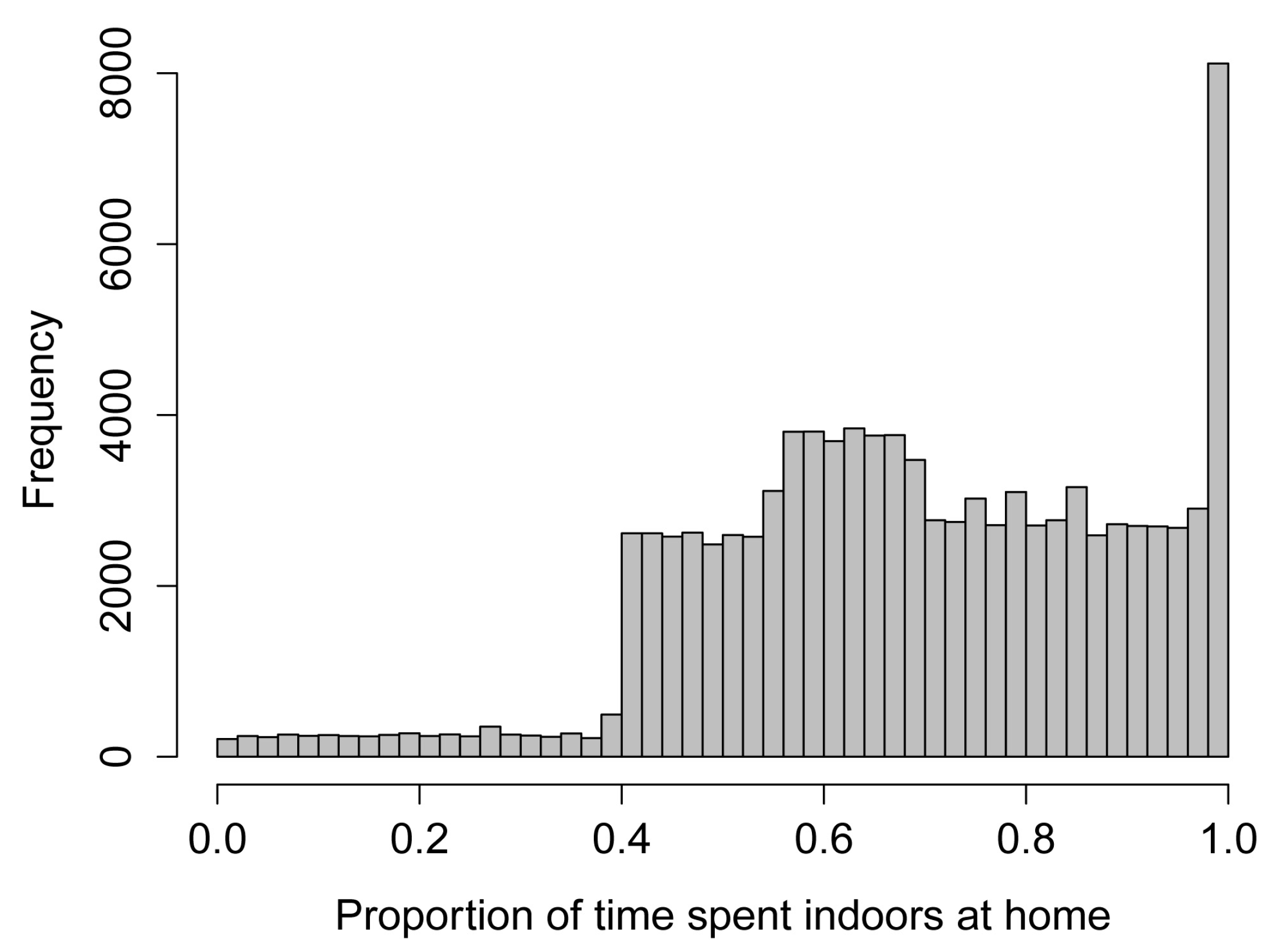
Evidence for the proportion of time spent away from the residence ( y ) is provided by the US National Human Activity Pattern Survey (NHAPS), a two year probability-based telephone survey of almost 10,000 people sponsored by the US EPA [28,29]. The survey found that, on average, individuals in the USA spend 68.7% of their time in a residence, 5.4% in an office or factory, 1.8% in a bar or restaurant, and 11% in other indoor locations: a total of 86.9% spent indoors, with the remaining time outdoors (7.6%) or in a vehicle (5.5%). These values were, on average, found to change relatively little in different parts of the US (±2%), despite the large climatic variations, and have remained fairly constant over recent decades. We used published percentiles for the time spent indoors at residences from the NHAPS data [30] to replicate the published (multimodal) distribution from the original survey data, as shown in Klepeis et al. (2001) [28] (Figure 3). Mortality in the ACS study will have been dominated by deaths in older people who spend a greater proportion of their time indoors. To account for this, as an approximation, we estimated the distributions of time spent indoors for individuals aged under 65 and over 65 based on the original survey data. These distributions were then combined into a single distribution that was weighted towards time spent indoors by people aged over 65, based on the proportion of deaths occurring in the two age groups using US life tables from the period of the ACS study.

3.2. Results of Simulations

We used the mean estimates of the three parameters described above ( r , F I N F and y ) to estimate the required mean adjustment to the ACS coefficient to reflect changes in the mortality risk for personal (Equation (8)) and residential indoor exposure to outdoor-generated PM2.5 (Equation (10)), and also a Monte Carlo simulation using 100,000 samples to make estimates for populations with different values of r , F I N F , and y (Table 3).
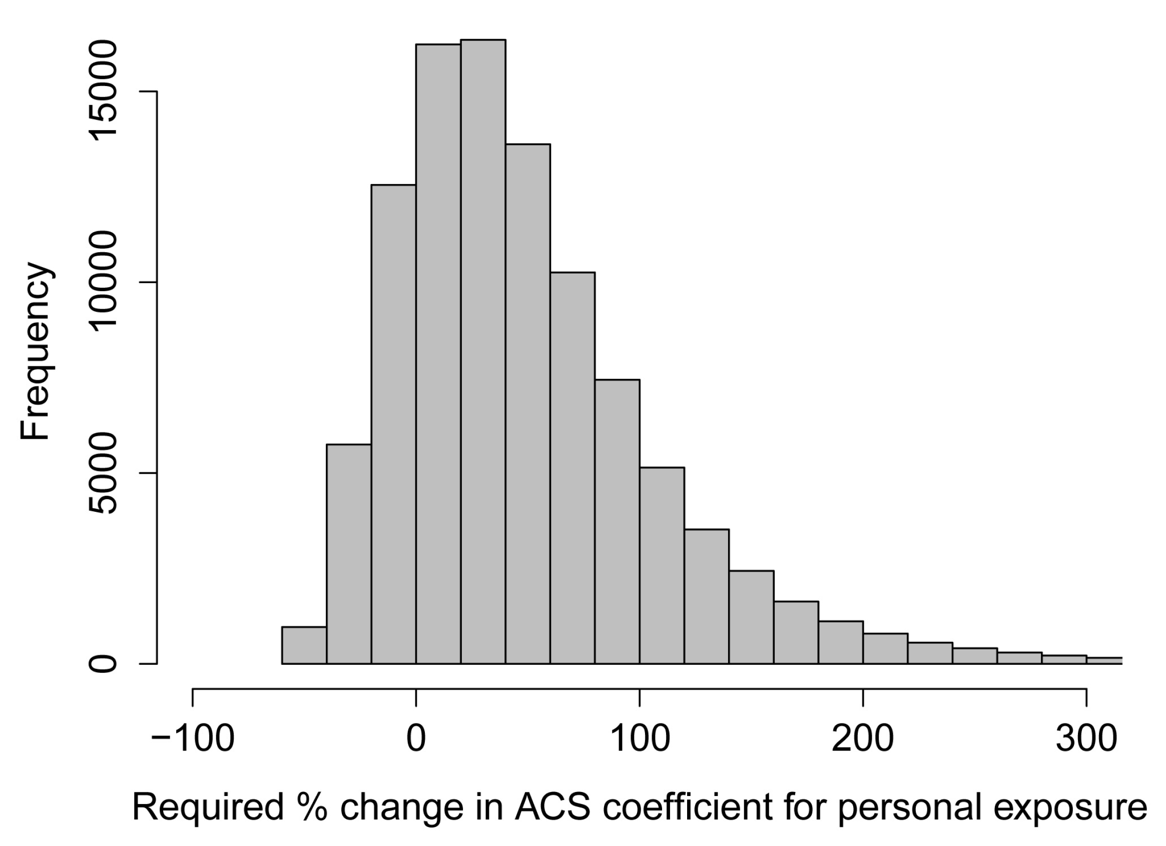
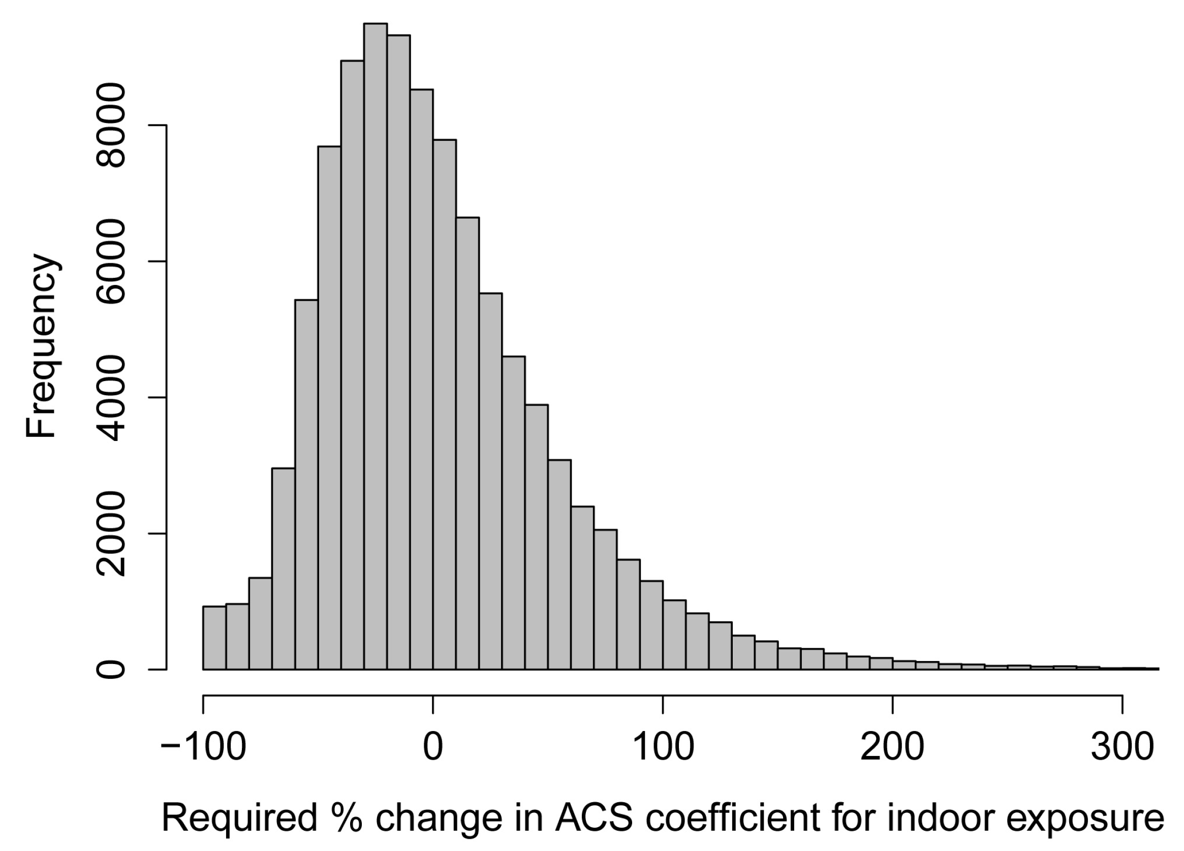
The results suggest that the required change to the ACS coefficient for personal exposure is a mean increase of 50.7% (median = 37.6%). This suggests that an appropriate multiplying factor may be around 1.3 to 1.5. However, for a coefficient for change in the indoor exposure to outdoor-generated PM2.5 ( C a i ), the fact that individuals spend some of their time outside the home means that a countervailing further adjustment is needed. The final impact on the relative risk (and hence the health impact calculation) is only modest (mean = 3.7%, median = −6.7%). Based on the median, it is worth noting that the required adjustment is a small decrease compared to the result that would be obtained by the application of the unadjusted ACS coefficient. Simulations assuming greater spatial variation in ambient PM2.5 (ratio of PM2.5 at the place of residence compared with at the monitoring location modelled using a log-normal distribution with standard deviation = 0.2) resulted in only a modest increase in the required adjustments for personal exposure (mean = 60.6%, median = 40.5%) and indoor exposure (mean = 10.5%, median = −5.8%).
The simulations suggest a high level of population variance in the required adjustments for both personal and indoor exposure. An appropriate relative risk for personal exposure in the ACS study is increased relative to the original ACS coefficient under most circumstances (Figure 4). However, for indoor exposure, although the relative risk may be marginally decreased on average, there is the potential for much more substantial changes to the coefficient (Figure 5). The proportion of time that individuals spend indoors at home is extremely important in this respect. For population groups who spend most or all of their time indoors, an increase in the ACS coefficient is required to assess changes in indoor PM2.5 exposure. The age-dependent analysis demonstrates this through the increases which would be required for infants (age four and under) and the elderly (age 65 and above) (Table 3).

4. Discussion

We have sought to establish the theoretical basis for using published exposure-response coefficients from studies with fixed-site monitors for exposure assignment in the calculation of the long-term health impacts associated with housing interventions that affect indoor air quality. Reassuringly, for fine particle exposures, the net result of adjustments appears to be fairly close to the value that would be obtained by the application of the unadjusted coefficient to changes in indoor PM2.5 due to outdoor sources ( C a i ). The change in mortality risk in relation to changes in personal exposure is appreciably greater (30–50%) than the original ACS coefficient indicates, but the fact that indoor PM2.5 is only a partial determinant of overall PM2.5 exposure tends to reduce the overall relative “correction” for residential indoor exposure to approximately unity. A modification to the ACS coefficient of around 30% to 50% for total personal exposure is broadly consistent with previously published evidence suggesting increased coefficients for personal exposure in time-series studies [37,38]. Similarly, studies adjusting coefficients for exposure measurement error using regression calibration techniques have tended to suggest that central monitoring sites generally provide a reasonable representation of overall personal exposures [39,40,41]. However, regression calibration requires detailed information on personal exposures (for instance, based on personal monitoring or remotely sensed data), which commonly does not account for indoor exposures. To address this gap, our method provides a logical rationale for scaling coefficients for use in indoor environments based on assumptions about the relationship between exposures indoors and at central monitoring sites.
On average, our results suggest that only a minor adjustment to the ACS coefficient is required for indoor exposure and so, in many circumstances, it is appropriate to apply the original ACS coefficient to assess changes in indoor PM2.5 from outdoor sources (without further adjustment for time spent indoors since this has been accounted for). Correction for specific population groups who spend a larger proportion of their time indoors may still be important, however, depending on where the HIA is applied. Our results suggest an upward correction of 10–20% may be required for assessing changes in the indoor exposures of infants and elderly people. It should be noted that different scaling factors would be needed for different sizes of particles due to differences in their ability to penetrate the building envelope and deposition velocities [27,42]. There is also evidence, though based on an analysis of short-term associations, to suggest further effect modification may occur due to specific seasonal and regional influences [43].
Of course, our calculations entail many assumptions. The assumption of a constant ratio of indoor PM2.5 from outdoor sources to outdoor PM2.5 ( F I N F ) (assumption 1) is reasonable and obtained when modelling software such as CONTAM is used to estimate the effect of housing interventions. Moreover, there are measurements in the literature to provide a reasonable basis for estimating the ratio, at least for some types of dwellings. In the absence of significant indoor sources, indoor and outdoor PM2.5 levels are generally observed to track each other fairly closely over time with indoor concentrations lower than outdoors [44,45]. Relatively few studies have attempted to quantify explicitly the contribution of ambient PM2.5 to indoor concentrations [46]. However, measurements in a dwelling in California have demonstrated that indoor PM2.5 of an outdoor origin represents on average around half the outdoor concentration [47].
The independence of time spent indoors vs. the infiltration ratio (assumption 2) is likely to be an oversimplification as people spend more time outdoors in warmer weather and are likely to open windows more, which will affect air exchange with the outdoors. Therefore, if people spend more time outdoors, the infiltration ratio ( F I N F ) will approach 1 (same concentration of indoor PM2.5 of outdoor origin as outdoor PM2.5), and the scaling factor for personal exposure ( β * ) will approach 1 / r (Equation (8)) and tend towards β (i.e., little or no change to the original ACS coefficient). However, in colder weather, the converse is true and the change to the coefficient for personal exposure will increase. As such, our judgement is that the degree to which there is a lack of independence is not critical to the overall conclusions of our study.
Assumption (3) is a simplification in particular because it assumes that the pollution outside the home is broadly representative of all non-dwelling-related PM2.5 exposure. This assumes that there is no spatial variability in outdoor PM2.5 (apart from a constant difference in PM2.5 concentrations between the monitoring site and any residence in a city) and disregards exposure in other microenvironments (such as transient microenvironments where concentrations of certain pollutants can be very high). For this reason, personal exposures tend to be higher than both outdoor and indoor (static) concentrations [25]. The model could be extended to provide a more complete representation of total personal exposure to PM2.5, going beyond a simple distinction of indoor and outdoor exposure, to separate exposure outside the home into components near the place of residence and those further afield, including in other (e.g., work- and transport-related) microenvironments. This would require a more complex exposure model including detailed information on exposures and time spent in all locations. However, because exposures in these other settings are not affected by dwelling characteristics or housing modifications, this assumption probably only leads to modest imprecision.
Our analysis has focused on housing in the USA, though similar arguments would apply in other settings. Dwelling characteristics, and particularly energy efficiency interventions, will clearly affect concentrations of particles derived from indoor sources because of their influence on ventilation. However, this raises a fundamental issue about the toxicity and health impact of particles derived from indoor sources. Our interpretation is that there is as yet insufficient evidence to draw a firm conclusion about the relative toxicity of particles of an indoor and outdoor origin [48]. The effect of our assumption (2) is to make clear that the application of the adjusted PM2.5-mortality coefficient is solely for that component of indoor PM2.5 derived from outdoor air and not of indoor PM2.5 in total. How indoor particle sources should be treated has a potentially larger impact than the adjustment of the coefficient for PM2.5 applied to fine particles of an outdoor origin. We think this is an important evidence gap of considerable public health importance, which means that current studies may not adequately address all components of the health impact relating to particle exposure.
In conclusion, the exposure-response functions derived from semi-ecological cohort studies may need to be adjusted when applying them to models of the health impact of changes in indoor particle concentrations from an outdoor origin. In general, our estimates suggest the required adjustment is relatively modest and hence the use of unadjusted coefficients is appropriate under many circumstances. However, existing coefficients should be adjusted when used for assessments of certain population groups, in particular vulnerable individuals such as infants and the elderly who spend a greater proportion of their time indoors at home.

Acknowledgments

The research leading to these results has received funding from the European Union Seventh Framework Programme FP7/2007-2013 under grant agreement No. 265325 (“PURGE”). The work was also carried out as part of the project “Pollutants in the Urban Environment: An Integrated Framework for Improving Sustainability of the Indoor Environment (PUrE Intrawise)”, funded by EPSRC (Grant no. EP/F007132/1). The authors gratefully acknowledge this funding and the support of other project partners.

Author Contributions

P.W. conceived the model. P.W. and B.A. refined and developed the model. Z.C. and J.M. developed the Monte Carlo simulation method. J.M., C.S., I.R., and S.V. assessed the evidence used to parameterize the model. J.M. performed the model simulations. P.W. and M.D. were project leaders and designed the study. J.M. and P.W. wrote the first draft of the paper. All authors contributed to the final paper.

Conflicts of Interest

The authors declare no conflict of interest. The founding sponsors had no role in the design of the study; in the collection, analyses, or interpretation of data; in the writing of the manuscript, and in the decision to publish the results.

References

  1. Wilkinson, P.; Smith, K.R.; Davies, M.; Adair, H.; Armstrong, B.G.; Barrett, M.; Bruce, N.; Haines, A.; Hamilton, I.; Oreszczyn, T.; et al. Public health benefits of strategies to reduce greenhouse-gas emissions: Household energy. Lancet 2009, 374, 1917–1929. [Google Scholar] [CrossRef]
  2. Vardoulakis, S.; Dimitroulopoulou, S.; Thornes, J.E.; Lai, K.-M.; Taylor, J.; Myers, I.; Heaviside, C.; Mavrogianni, A.; Shrubsole, C.; Chalabi, Z.; et al. Impact of climate change on the domestic indoor environment and associated health risks in the UK. Environ. Int. 2015, 85, 299–313. [Google Scholar] [CrossRef] [PubMed]
  3. Shrubsole, C.; Ridley, I.; Biddulph, P.; Milner, J.; Vardoulakis, S.; Ucci, M.; Wilkinson, P.; Chalabi, Z.; Davies, M. Indoor PM2.5 exposure in London’s domestic stock: Modelling current and future exposures following energy efficient refurbishment. Atmos. Environ. 2012, 62, 336–343. [Google Scholar] [CrossRef]
  4. Milner, J.; Shrubsole, C.; Das, P.; Jones, B.; Ridley, I.; Chalabi, Z.; Hamilton, I.; Armstrong, B.; Davies, M.; Wilkinson, P. Home energy efficiency and radon related risk of lung cancer: Modelling study. BMJ 2014, 348, f7493. [Google Scholar] [CrossRef] [PubMed]
  5. Broderick, Á.; Byrne, M.; Armstrong, S.; Sheahan, J.; Coggins, A.M. A pre and post evaluation of indoor air quality, ventilation, and thermal comfort in retrofitted co-operative social housing. Build. Environ. 2017, 122, 126–133. [Google Scholar] [CrossRef]
  6. COMEAP. Long-Term Exposure to Air Pollution: Effect on Mortality; The Stationary Office: London, UK, 2009.
  7. COMEAP. The Mortality Effects of Long-Term Exposure to Particulate Air Pollution in the United Kingdom; The Stationary Office: London, UK, 2010.
  8. Pope, C.A., III; Burnett, R.T.; Thun, M.J.; Calle, E.E.; Krewski, D.; Ito, K.; Thurston, G.D. Lung cancer, cardiopulmonary mortality, and long-term exposure to fine particulate air pollution. JAMA 2002, 287, 1132–1141. [Google Scholar] [CrossRef] [PubMed]
  9. Pope, C.A., III; Burnett, R.; Krewski, D.; Jerrett, M.; Shi, Y.; Calle, E.E.; Thun, M.J. Cardiovascular mortality and exposure to airborne fine particulate matter and cigarette smoke: Shape of the exposure-response relationship. Circulation 2009, 120, 941–948. [Google Scholar] [CrossRef] [PubMed]
  10. Pope, C.A., III; Burnett, R.T.; Turner, M.C.; Cohen, A.; Krewski, D.; Jerrett, M.; Gapstur, S.M.; Thun, M.J. Lung cancer and cardiovascular disease mortality associated with ambient air pollution and cigarette smoke: Shape of the exposure-response relationships. Environ. Health Perspect. 2011, 119, 1616–1621. [Google Scholar] [CrossRef] [PubMed]
  11. US EPA. Quantitative Health Risk Assessment for Particulate Matter; US Environmental Protection Agency: Research Triangle Park, NC, USA, 2010.
  12. Milner, J.; Vardoulakis, S.; Chalabi, Z.; Wilkinson, P. Modelling inhalation exposure to combustion-related air pollutants in residential buildings: Application to health impact assessment. Environ. Int. 2011, 37, 268–279. [Google Scholar] [CrossRef] [PubMed]
  13. Schwartz, J.; Laden, F.; Zanobetti, A. The concentration-response relation between PM2.5 and daily deaths. Environ. Health Perspect. 2002, 110, 1025–1029. [Google Scholar] [CrossRef] [PubMed]
  14. Koistinen, K.J.; Edwards, R.D.; Mathys, P.; Ruuskanen, J.; Kunzli, N.; Jantunen, M.J. Sources of fine particulate matter in personal exposures and residential indoor, residential outdoor and workplace microenvironments in the Helsinki phase of the EXPOLIS study. Scand. J. Work Environ. Health 2004, 30, 36–46. [Google Scholar]
  15. Ji, W.; Zhao, B. Estimating mortality dervied from indoor exposure to particles of outdoor origin. PLoS ONE 2015, 10, e0124238. [Google Scholar]
  16. Hosgood, H.D.I.; Boffetta, P.; Greenland, S.; Lee, Y.C.; McLaughlin, J.; Seow, A. In-home coal and wood use and lung cancer risk: A pooled analysis of the International Lung Cancer Consortium. Environ. Health Perspect. 2010, 118, 1743–1747. [Google Scholar] [CrossRef] [PubMed]
  17. Lim, S.S.; Vos, T.; Flaxman, A.D.; Danaei, G.; Shibuya, K.; Adair-Rohani, H.; Al Mazroa, M.A.; Amann, M.; Anderson, H.R.; Andrews, K.G.; et al. A comparative risk assessment of burden of disease and injury attributable to 67 risk factors and risk factor clusters in 21 regions, 1990—2010: A systematic analysis for the Global Burden of Disease study 2010. Lancet 2012, 380, 2224–2260. [Google Scholar] [CrossRef]
  18. U.S. Department of Health and Human Services. The Health Consequences of Involuntary Exposure to Tobacco Smoke: A Report of the Surgeon General; U.S. Dept. of Health and Human Services, Centers for Disease Control and Prevention, Coordinating Center for Health Promotion, National Center for Chronic Disease Prevention and Health Promotion, Office on Smoking and Health: Atlanta, GA, USA, 2006.
  19. Ebelt, S.T.; Wilson, W.E.; Brauer, M. Exposure to ambient and nonambient components of particulate matter: A comparison of health effects. Epidemiology 2005, 16, 396–405. [Google Scholar] [CrossRef]
  20. Long, C.M.; Suh, H.H.; Kobzik, L.; Catalano, P.J.; Ning, Y.Y.; Koutrakis, P. A pilot investigation of the relative toxicity of indoor and outdoor fine particles: In vitro effects of endotoxin and other particulate properties. Environ. Health Perspect. 2001, 109, 1019–1026. [Google Scholar] [CrossRef] [PubMed]
  21. Rohr, A.C.; Wyzga, R.E. Attributing health effects to individual particulate matter constituents. Atmos. Environ. 2012, 62, 130–152. [Google Scholar] [CrossRef]
  22. Stanek, L.W.; Sacks, J.D.; Dutton, S.J.; Dubois, J.-J.B. Attributing health effects to apportioned components and sources of particulate matter: An evaluation of collective results. Atmos. Environ. 2011, 45, 5655–5663. [Google Scholar] [CrossRef]
  23. Wilson, W.E.; Mage, D.T.; Gran, L.D. Estimating separately personal exposure to ambient and nonambient particulate matter for epidemiology and risk assessment: Why and how. J. Air Waste Manag. Assoc. 2000, 50, 1167–1183. [Google Scholar] [CrossRef] [PubMed]
  24. Feller, W. Random variables; expectation. In An Introduction to Probability Theory and Its Applications, 3rd ed.; Wiley International: New York, NY, USA, 1968; Volume 1. [Google Scholar]
  25. Adgate, J.L.; Mongin, S.J.; Pratt, G.C.; Zhang, J.; Field, M.P.; Ramachandran, G.; Sexton, K. Relationships between personal, indoor, and outdoor exposures to trace elements in PM(2.5). Sci. Total Environ. 2002, 386, 21–32. [Google Scholar] [CrossRef] [PubMed]
  26. Ozkaynak, H.; Xue, J.; Spengler, J.; Wallace, L.; Pellizzari, E.; Jenkins, P. Personal exposure to airborne particles and metals: Results from the Particle TEAM study in Riverside, California. J. Expo. Anal. Environ. Epidemiol. 1996, 6, 57–78. [Google Scholar] [PubMed]
  27. Wallace, L. Indoor particles: A review. J. Air Waste Manag. Assoc. 1996, 46, 98–126. [Google Scholar] [CrossRef] [PubMed]
  28. Klepeis, N.E.; Nelson, W.C.; Ott, W.R.; Robinson, J.P.; Tsang, A.M.; Switzer, P.; Behar, J.V.; Hern, S.C.; Engelmann, W.H. The National Human Activity Pattern Survey (NHAPS): A resource for assessing exposure to environmental pollutants. J. Expo. Anal. Environ. Epidemiol. 2001, 11, 231–252. [Google Scholar] [CrossRef] [PubMed]
  29. Klepeis, N.E.; Tsang, A.M.; Behar, J.V. Analysis of the National Human Activity Pattern Survey (NHAPS) Respondents from a Standpoint of Exposure Assessment. Final Report; US EPA: Las Vegas, NV, USA, 1995.
  30. Tsang, A.M.; Klepeis, N.E. Descriptive Statistics Tables from a Detailed Analysis of the National Human Activity Pattern Survey (NHAPS) Data; U.S. Environmental Protection Agency: Washington, DC, USA, 1996.
  31. Ott, W.; Wallace, L.; Mage, D. Predicting particulate (PM10) personal exposure distributions using a random component superposition statistical model. J. Air Waste Manag. Assoc. 2000, 50, 1390–1406. [Google Scholar] [CrossRef] [PubMed]
  32. Rodes, C.E.; Lawless, P.A.; Thornburg, J.W.; Williams, R.W.; Croghan, C.W. DEARS particulate matter relationships for personal, indoor, outdoor, and central site settings for a general population. Atmos. Environ. 2010, 44, 1386–1399. [Google Scholar] [CrossRef]
  33. Goswami, E.; Larson, T.; Lumley, T.; Liu, L.J. Spatial characteristics of fine particulate matter: Identifying representative monitoring locations in Seattle, Washington. J. Air Waste Manag. Assoc. 2002, 52, 324–333. [Google Scholar] [CrossRef] [PubMed]
  34. Meng, Q.Y.; Turpin, B.J.; Korn, L.; Weisel, C.P.; Morandi, M.; Colome, S.; Zhang, J.J.; Stock, T.; Spektor, D.; Winer, A.; et al. Influence of ambient (outdoor) sources on residential indoor and personal PM2.5 concentrations: Analyses of RIOPA data. J. Expo. Anal. Environ. Epidemiol. 2005, 15, 17–28. [Google Scholar] [CrossRef] [PubMed]
  35. Diapouli, E.; Chaloulakou, A.; Koutrakis, P. Estimating the concentration of indoor particles of outdoor origin: A review. J. Air Waste Manag. Assoc. 2013, 63, 1113–1129. [Google Scholar] [CrossRef] [PubMed]
  36. Emmerich, S. Validation of multizone IAQ modeling of residential-scale buildings: A review. ASHRAE Trans. 2001, 107, 619–628. [Google Scholar]
  37. Zeger, S.L.; Thomas, D.; Dominici, F.; Samet, J.M.; Schwartz, J.; Dockery, D.; Cohen, A. Exposure measurement error in time-series studies of air pollution: Concepts and consequences. Environ. Health Perspect. 2000, 108, 419–426. [Google Scholar] [CrossRef] [PubMed]
  38. Avery, C.L.; Mills, K.T.; Williams, R.; McGraw, K.A.; Poole, C.; Smith, R.L.; Whitsel, E.A. Estimating error in using ambient PM2.5 concentrations as proxies for personal exposures: A review. Epidemiology 2010, 21, 215–223. [Google Scholar] [CrossRef] [PubMed]
  39. Kioumourtzoglou, M.-A.; Spiegelman, D.; Szpiro, A.A.; Sheppard, L.; Kaufman, J.D.; Yanosky, J.D.; Williams, R.; Laden, F.; Hong, B.; Suh, H. Exposure measurement error in PM2.5 health effects studies: A pooled analysis of eight personal exposure validation studies. Environ. Health 2014, 3, 2. [Google Scholar] [CrossRef]
  40. Hart, J.E.; Liao, X.; Hong, B.; Puett, R.C.; Yanosky, J.D.; Suh, H.; Kioumourtzoglou, M.-A.; Spiegelman, D.; Laden, F. The association of long-term exposure to PM2.5 on all-cause mortality in the Nurses’ Health Study and the impact of measurement-error correction. Environ. Health 2015, 14, 38. [Google Scholar] [CrossRef] [PubMed]
  41. Jerrett, M.; Turner, M.C.; Beckerman, B.S.; Pope, C.A., III; van Donkelaar, A.; Martin, R.V.; Serre, M.; Crouse, D.; Gapstur, S.M.; Krewski, D.; et al. Comparing the health effects of ambient particulate matter estimated using ground-based versus remote sensing exposure estimates. Environ. Health Perspect. 2017, 125, 552–559. [Google Scholar] [CrossRef] [PubMed]
  42. Long, C.M.; Suh, H.H.; Koutrakis, P. Characterization of indoor particle sources using continuous mass and size monitors. J. Air Waste Manag. Assoc. 2000, 1236–1250. [Google Scholar] [CrossRef]
  43. Chen, C.; Zhao, B.; Weschler, C.J. Indoor exposure to “outdoor PM10”: Assessing its influence on the relationship between PM10 and short-term mortality in U.S. Cities. Epidemiology 2012, 23, 870–878. [Google Scholar] [CrossRef] [PubMed]
  44. Lazaridis, M.; Aleksandropoulou, V.; Smolik, J.; Hansen, J.E.; Glytsos, T.; Kalogerakis, N.; Dahlin, E. Physico-chemical characterization of indoor/outdoor particulate matter in two residential houses in Oslo, Norway: Measurements overview and physical properties—URBAN-AEROSOL Project. Indoor Air 2006, 16, 282–295. [Google Scholar] [CrossRef] [PubMed]
  45. Monn, C.; Fuchs, A.; Hogger, D.; Junker, M.; Kogelschatz, D.; Roth, N.; Wanner, H.U. Particulate matter less than 10 microns (PM10) and fine particles less than 2.5 microns (PM2.5): Relationships between indoor, outdoor and personal concentrations. Sci. Total Environ. 1997, 208, 15–21. [Google Scholar] [CrossRef]
  46. Taylor, J.; Shrubsole, C.; Davies, M.; Biddulph, P.; Das, P.; Hamilton, I.; Vardoulakis, S.; Mavrogianni, A.; Jones, B.; Oikonomou, E. The modifying effect of the building envelope on population exposure to PM2.5 from outdoor sources. Indoor Air 2014, 24, 639–651. [Google Scholar] [CrossRef] [PubMed]
  47. Kopperud, R.J.; Ferro, A.R.; Hildemann, L.M. Outdoor versus indoor contributions to indoor particulate matter (PM) determined by mass balance methods. J. Air Waste Manag. Assoc. 2004, 54, 1188–1196. [Google Scholar] [CrossRef] [PubMed]
  48. Abdullahi, K.L.; Delgado-Saborit, J.M.; Harrison, R.M. Emissions and indoor concentrations of particulate matter and its specific chemical components from cooking: A review. Atmos. Environ. 2013, 71, 260–294. [Google Scholar] [CrossRef]
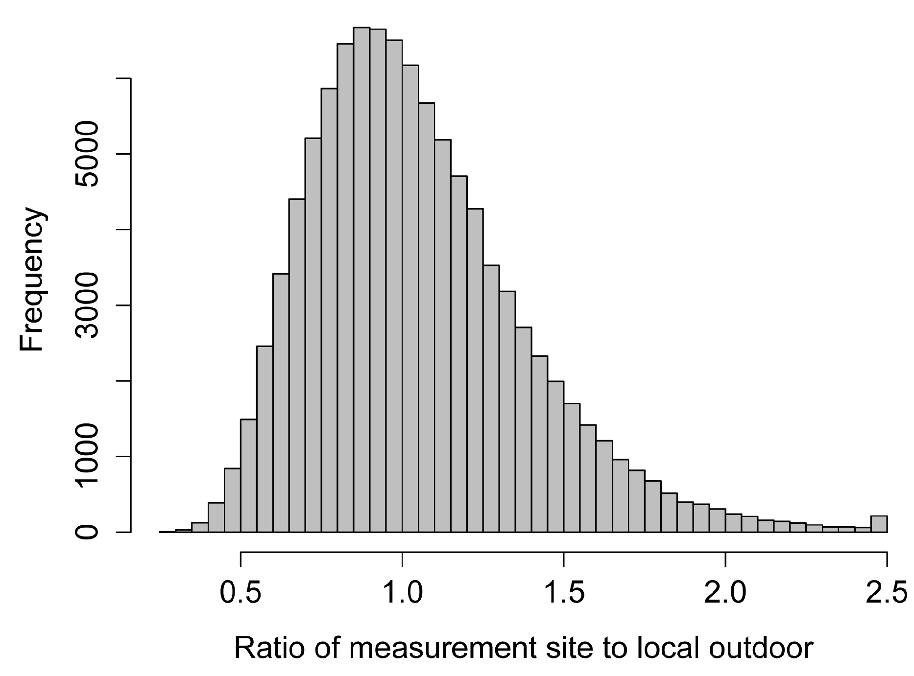
Figure 1. Estimated distribution of ratio of PM2.5 at measurement site to outdoor PM2.5 at residence (r) based on a Monte Carlo simulation (n = 100,000).
Climate 05 00066 g001
Figure 2. Estimated distribution of infiltration ratio (F_INF) based on a Monte Carlo simulation (n = 100,000).
Climate 05 00066 g002
Figure 3. Estimated distribution of time spent indoors by ACS population (y) based on a Monte Carlo simulation (n = 100,000).
Climate 05 00066 g003
Figure 4. Required percentage change in ACS coefficient for personal exposure to outdoor-generated PM2.5 based on a Monte Carlo simulation (n = 100,000).
Climate 05 00066 g004
Figure 5. Required percentage change in ACS coefficient for indoor exposure to outdoor-generated PM2.5 based on a Monte Carlo simulation (n = 100,000).
Climate 05 00066 g005
Table 1. Notation used for derivation.
SymbolDescription
C m PM2.5 concentration outdoors at the place of monitor (or average of monitors) *
C a PM2.5 concentration outdoors at the dwelling *
C a i PM2.5 concentration indoors due to infiltration from outdoors *
C i g PM2.5 concentration indoors due to indoor sources *
C i Overall PM2.5 concentration indoors *
E t Total personal exposure (PM2.5 concentration in breathing zone) *
r Ratio of PM2.5 at the dwelling compared with at the monitoring location ( C a / C m ) *
F I N F Infiltration ratio of indoor PM2.5 of outdoor origin to outdoor PM2.5 at the home ( C a i / C a ) *
y Proportion of time spent indoors at home *
y Proportion of time spent indoors at home for population in which HIA is to be performed
* For ACS study.
Table 2. Estimated parameter distributions and sources of evidence.
ParameterDistributionSource
ShapeMeanStandard Deviation
Ratio of PM2.5 concentration at a monitoring site to that in the outdoor air at the place of residence ( r )Log-normal distribution1.00.1Observed data on spatial variations in ambient PM2.5 [25] and analysis of monitoring sites in New York
Ratio of PM2.5 in the indoor air due to outdoor sources to that in the outside air ( F I N F )Beta distribution with shape parameters “alpha” = 5.12, “beta” = 2.520.670.16Measurements in US homes as part of the PTEAM study [26], as cited by Wallace (1996) [27]
Proportion of time spent indoors at home ( 1 y )Multimodal distribution (estimated by sampling using published percentiles)0.695 (0.802 *)0.191 (0.170 *)Survey data from the US National Human Activity Pattern Survey (NHAPS) [28,29,30]
* Weighted towards deaths in older age groups.
Table 3. Required change to the ACS coefficient for personal and indoor exposure to outdoor-generated PM2.5.
PM2.5 ExposureRequired Percentage Change to ACS Coefficient
MeanMedianStandard Deviation
Based on mean of r , F I N F and y
Personal exposure36.0%
Indoor exposure−5.5%
Probabilistic sampling from distributions of r , F I N F and y
Personal exposure50.7%37.6%66.4%
Indoor exposure
 Overall3.7%−6.7%56.5%
 Age-dependent
 Ages 1 to 425.7%14.5%62.6%
 Ages 5 to 114.3%−6.3%54.5%
 Ages 12 to 170.9%−9.2%54.0%
 Ages 18 to 64−2.0%−12.6%54.5%
 Ages 65 and above21.2%10.5%61.4%