Article

Utilizing Humidity and Temperature Data to Advance Monitoring and Prediction of Meteorological Drought

1
Jet Propulsion Laboratory, California Institute of Technology, Pasadena, CA 91109, USA
2
Department of Geography, Portland State University, Portland, OR 97201, USA
*
Author to whom correspondence should be addressed.
Climate 2015, 3(4), 999-1017; https://doi.org/10.3390/cli3040999
Submission received: 18 September 2015 / Revised: 4 November 2015 / Accepted: 12 November 2015 / Published: 18 November 2015
(This article belongs to the Special Issue Climate Extremes: Observations and Impacts)

Abstract

:
The fraction of land area over the Continental United States experiencing extreme hot and dry conditions has been increasing over the past several decades, consistent with expectation from anthropogenic climate change. A clear concurrent change in precipitation, however, has not been confirmed. Vapor pressure deficit (VPD), combining temperature and humidity, is utilized here as an indicator of the background atmospheric conditions associated with meteorological drought. Furthermore, atmospheric conditions associated with warm season drought events are assessed by partitioning associated VPD anomalies into the temperature and humidity components. This approach suggests that the concurrence of anomalously high temperature and low humidity was an important driver of the rapid development and evolution of the exceptionally severe 2011 Texas and the 2012 Great Plains droughts. By classification of a decade of extreme drought events and tracking them back in time, it was found that near surface atmospheric temperature and humidity add essential information to the commonly used precipitation-based drought indicators and can advance efforts to determine the timing of drought onset and its severity.

1. Introduction

Drought is a multifaceted climate phenomenon, often occurring at large spatial and temporal scales. In some notable cases, droughts can span multiple years and extend to continental spatial scales. Additionally, drought is associated with numerous severe societal impacts ranging from reduced water availability for human consumption to agricultural failure and famine. Furthermore, drought is often associated with other extreme weather and climate events, such as heatwaves and extreme temperatures [1,2,3], and is impacted by their changes [4]. As a result, drought is among the costliest of natural disasters [5,6]. Because of associated high societal costs, advanced forecasting of drought and associated extreme events can provide valuable information to aid in preparation [7]. One challenge to systematically improving forecasts is that drought onset, severity, duration, and areal extent may vary from one climate regime to another, requiring regional analysis of indicators used to determine drought occurrence and severity.
Drought, by definition, is simply a water deficit; however, the time scale over which water deficits accumulate can determine the type and impacts of drought. Drought indices must be associated with a specific time scale, as the response of hydrological systems to water deficit is time dependent [8,9,10]. Droughts are often categorized into meteorological, agricultural, or hydrological drought, and socio-economic impacts of each category may be realized at different space and time scales during the evolution of the event [11,12]. Meteorological drought is primarily characterized by a lack of precipitation over a prolonged time period, agricultural drought is primarily related to soil moisture and plant stress, and hydrological drought is often the result of extended precipitation shortfalls that impact the water supply (e.g., reservoirs, streamflow, and groundwater). Because meteorological drought typically precedes other types of drought, the multiscale feature of precipitation has formed the basis for the development of the standard precipitation index (SPI), which depends solely on precipitation [13], and has been widely used for drought monitoring and prediction [14,15,16,17,18]. To compute the SPI, the precipitation record for a given accumulation period is fitted to a probability distribution, which is then transformed into a normal distribution to determine the SPI value. SPI can thus be compared spatially and temporally across regions with markedly different climates. Positive SPI values correspond to wetter and negative to drier conditions in relation to the climatological mean.
While the multiscale feature of SPI is desirable, the index does not incorporate the role of temperature in future drought evolution. Using a general circulation model experiment, Abramopoulos et al. [19] showed that up to 80% of rainfall at the surface can be lost through evaporation and transpiration, illustrating the marked effects that temperature can have on drought severity. Because air temperature determines the atmospheric capacity for water vapor and thus significantly influences evapotranspiration (ET), it is important to consider both temperature and precipitation for drought monitoring [20,21,22,23] and prediction [17]. This also has substantial implications for future drought as global temperatures continue to rise. To address this, the Palmer Drought Severity Index (PDSI) and the standardized precipitation evapotranspiration index (SPEI; [24]) both account for temperature and precipitation and are thus more desirable than SPI for assessing and predicting drought in a warming climate [24,25].
The majority of studies focusing on drought rely on relatively simple measures to analyze temporary water deficit anomalies. However, it is also important to account for the background atmospheric humidity and temperature, as it relates to drought onset and development [11]. Recent studies show an overall drying trend on land coincident with and thermodynamically consistent with observed global warming [26,27,28,29,30,31]. Because of the limited availability of water for evaporation over land compared to the ocean, land surfaces warm about 50% more than ocean surfaces [29] and water vapor content cannot increase sufficiently fast to overcome this deficit. Therefore, further drying over land is expected as the climate continues to warm [32], resulting in a growing difference between actual and saturation water vapor concentrations. Consequently, the vapor pressure deficit (VPD), which also controls evapotranspiration demand, would increase much faster by percentage than changes in other hydrological variables such as precipitation [32,33]. In this case, even regions that may receive more rain in the future could experience an overall increase in water deficit [34].
Relative humidity (RH), defined as the actual water vapor partial pressure (e) divided by saturated water vapor pressure (es), can be used to assess atmospheric aridity. Another alternative is VPD, defined as the differences between es and e (es-e), providing an absolute measure of the ability of the atmosphere to wick moisture from the land surface and vegetation. Seager et al. [35] showed that at very low temperatures a given RH will correspond to a very small VPD while at high temperatures the same RH will correspond to a very high VPD, so a combination of low RH and high temperature makes VPD a robust measure for identifying high fire danger conditions. Williams et al. [36] show that VPD can explain more variance than precipitation in linking climate and forest fire occurrence and Lobell et al. [37] found that VPD is a robust variable to assess the sensitivity of crop yield to drought.
In the present work, the impact of key atmospheric state variables (temperature and moisture) in the development of drought is investigated over the Continental United States (CONUS) through long-term assessment and case studies. This analysis employs VPD and also dissects it into temperature and humidity components to further assess the role of the components in the formation and intensification of the events and to show the impact of ignoring temperature and humidity in the drought assessment. The data used in this study are described in Section 2. Results and concluding remarks are provided in Section 3 and Section 4, respectively.

2. Data and Methodology

2.1. Data

2.1.1. PRISM

Gridded observations of near-surface air temperature, dewpoint temperature, and precipitation are obtained from the Parameter-elevation Regressions on Independent Slopes Model (PRISM) dataset [38,39] developed by the PRISM Climate Group at Oregon State University. PRISM data are high quality meteorological station observations interpolated to a 4-km grid using a human expert and statistical knowledge-based system that utilizes a digital elevation model [39] (http://www.prism.oregonstate.edu). The PRISM data employed in this study have a monthly temporal resolution and are available starting at 1895 over the CONUS. For this analysis, we only use data from 1900 onward.

2.1.2. U.S. Drought Monitor (USDM)

The U.S. Drought Monitor (USDM; http://droughtmonitor.unl.edu/) is a composite product including climate indices, numerical models, and inputs from regional and local experts [40]. While the USDM drought maps may not be considered as ground “truth”, they can provide a composite perspective of drought from onset (typically first identified via meteorological drought indices) to recovery. USDM drought maps have been used in a variety of studies [40,41] and provide five categories of drought severity: D0 (abnormally dry), D1 (moderate drought), D2 (severe drought), D3 (extreme drought), and D4 (exceptional drought). The five drought categories are provided every week at sub-kilometer grids and approximately correspond to the following thresholds of the SPI: −0.5 to −0.7 (D0), −0.8 to −1.2 (D1), −1.3 to −1.5 (D2), −1.6 to −1.9 (D3), and −2.0 or less (D4). In the present work both datasets are mapped onto a common 0.1 × 0.1-degree resolution at monthly time scales prior to analysis.

2.2. Method

The impact of atmospheric temperature and moisture on drought development and implications for monitoring are investigated. This is performed through a combination of case studies and analyses of an ensemble of extreme drought events as described in Section 3. We calculated 3-month SPI (SPI3), 3-month SPEI (SPEI3), and VPD (hereafter referred as SVPD3). The standardization approach is described in Section 2.2.2. It should be noted that shorter time scales tend to have nonnormal precipitation frequency distributions in arid climates [42] and, due to hydrologic delays in snow pack-forming regions, linking short term accumulation of precipitation indices to drought may not be reasonable [43]. Similar to Vicente-Serrano et al. [12], potential evapotranspiration is calculated using the Thornthwaite method [44] requiring surface air temperature. Both SPI and SPEI are obtained by transforming the cumulative probability of the precipitation and precipitation minus evapotranspiration using the inverse of the standard normal distribution and by incorporating the entire record (1900–2013). VPD is calculated using monthly surface air temperature (Tmean in °C) and dewpoint temperature (Tdmean in °C) and the following equation:
VPD = c 1 × exp ( c 2 × T m e a n c 3 + T m e a n ) + c 1   exp ( c 2   × T d m e a n c 3 + T d m e a n )
Here, c1 = 0.611 kPa, c2 = 17.5, c3 = 240.978 °C and VPD is in kPa. Weiss et al. [45] examined the monthly versus daily calculations of VPD, and found that monthly mean VPD values based on monthly mean temperature and dew point is reliably consistent with monthly mean VPD calculated from daily VPD values. A similar conclusion was reported by Seager et al. [35].

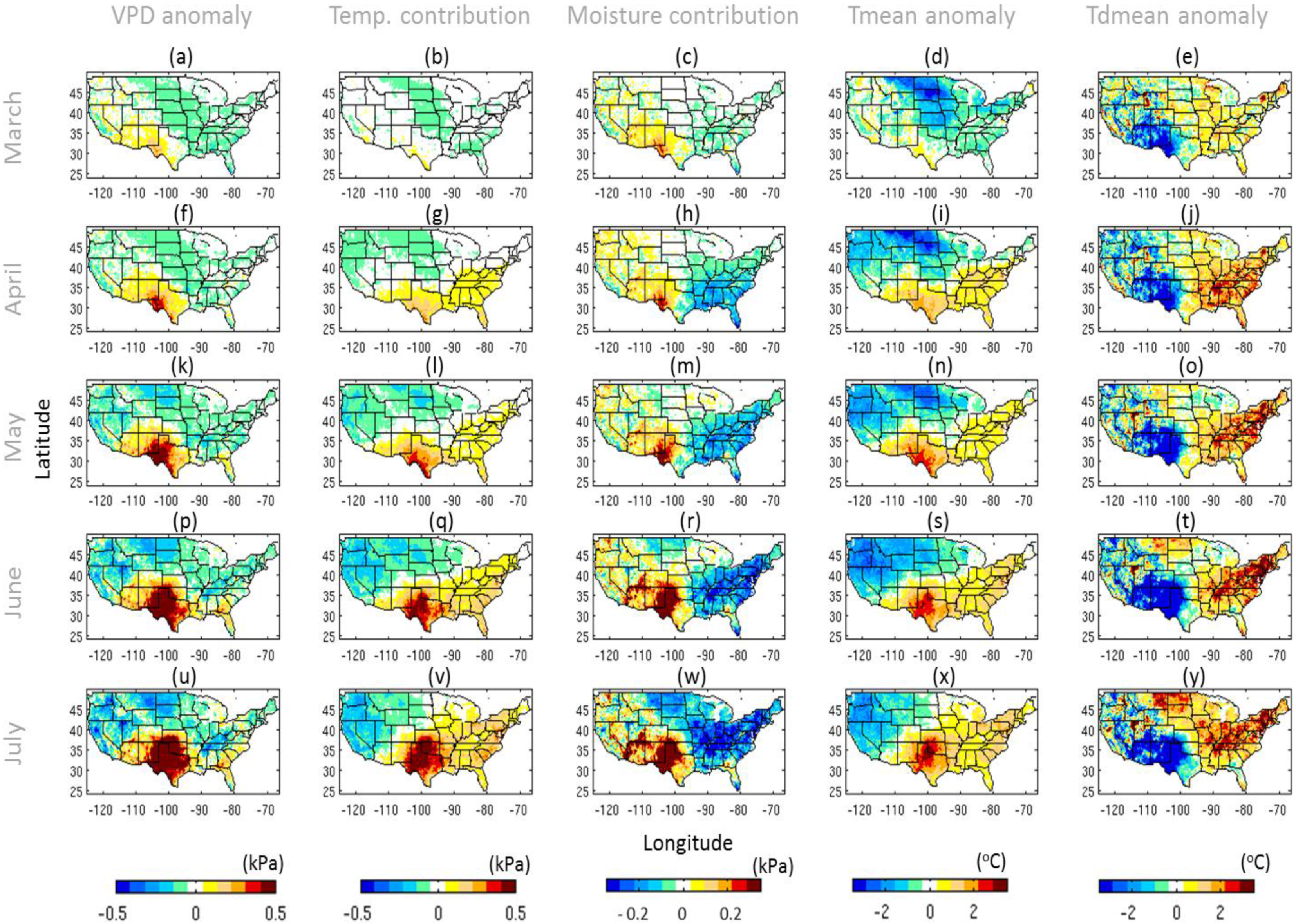
2.2.1. Dissection of VPD Associated with Drought Events

In order to better understand the relative contribution of temperature and humidity to VPD in a given drought event, a method similar to that used by Weiss et al. [46] is implemented for each drought event. Calculating VPD from Equation (1) using Tmean of a drought event, together with climatological Tdmean (i.e., calculated from the entire record), shows the contribution of temperature to the VPD during the event. Similarly, if climatological Tmean is used together with Tdmean of a drought event, the contribution of the atmospheric moisture (captured by Tdmean) to the event’s evapotranspiration demand is obtained. In this study the dissection approach is applied to two case studies, using the entire data record for climatological means, to assess the relative contribution of temperature and moisture to VPD and how they change with time as drought develops. A simple k-means classification is then applied to the contributing moisture and temperature components to identify different atmospheric states under which drought develops. We demonstrate that understanding atmospheric conditions is important for assessing the efficacy of different drought indices in the monitoring and prediction of regional droughts.

2.2.2. Calculation of Standardized Indices

To compare VPD to other commonly used drought indicators, we also compute standardized indices of precipitation, precipitation minus evapotranspiration, and temperature. The standardization allows for comparisons between different locations with different climates [13] and at various timescales. In previous studies, standardization has also been applied to other variables such as soil moisture, runoff, and precipitation minus evapotranspiration [12,43] facilitating inter-comparison of different drought indices. In the SPI, the gamma distribution is often used to calculate the cumulative probability distribution of precipitation, followed by transformation using the inverse of the standard normal distribution [13]. Empirical cumulative probability distributions, such as the Weibull plotting position formula, have also been used to estimate the SPI or soil moisture percentiles [47,48,49]. The use of empirical cumulative probability distributions helps avoid assumptions regarding the distribution family, reduce computational burden in fitting parametric distributions, and facilitates calculating standardized indices for various variables. Here, an empirical approach is used to derive the marginal probability [50] using the following univariate form of the Gringorten plotting position formula [51]:
P ( x i ) = i 0.44 n + 0.12
where i is the rank of the observed values from the smallest, and n is the number of the observations. Comparative analysis using SPI shows that the SPI calculated from a gamma distribution and that based on Equation (2) yield almost identical results. Therefore, for comparative analysis, the empirical approach is applied to different variables investigated in this study.

3. Results

3.1. CONUS Drought Probability

Figure 1a–d shows seasonal maps of the probability of severe drought calculated from 11 years (2003–2013) as defined by months exceeding category D2 of the USDM. The USDM based drought probability maps suggest that severe droughts are most frequent over western CONUS, and that the probability of drought is generally higher in summer than other seasons. Severe drought probability maps are also constructed based on SPI3 (panels e–h) and SPEI3 (panels i–l) and by applying the threshold −1.25, corresponding to USDM drought category 2 as noted in the USDM classification table (http://droughtmonitor.unl.edu/AboutUs/ClassificationScheme.aspx). Both SPI3 and SPEI3 are calculated using the entire-year record (1900–2013), but the probability maps are calculated using a subset of the record (the same 11 years utilized in the USDM probability maps). Drought probability maps based on SPI3 and SPEI3 also show that recent severe droughts are generally more frequent in the western and southwestern CONUS, but with a lower frequency than those identified by USDM. This is likely because, in addition to meteorological drought, USDM accounts for agricultural and hydrological droughts that can occur consecutively. Thus, USDM drought maps are more persistent than those based on only meteorological droughts. SPI and SPEI are typically used to monitor meteorological drought, the onset of which can often be captured earlier than other drought types.
Figure 1. Seasonal maps of probability of severe drought identified based on (ad) USDM drought categories equal or greater than 2, (eh) SPI3 < −1.25, (il) SPEI3 < −1.25, and (mp) SVPD3 > 1.25. Columns, from left to right, the seasons are winter (DJF), spring (MAM), summer (JJA), and fall (SON). The probabilities are calculated using the latest 11 years (2003–2013), but for calculation of standardized indices the entire record (1900–2013) is used.
Climate 03 00999 g001
SPEI3 maps (Figure 1i–l) indicate that severe drought is most frequent in summer and fall and most often observed over the Southwestern U.S. However, little discernable seasonal variation is observed in drought probability maps based on SPI3 (Figure 1e–h). Furthermore, SPI3 and SPIE3 maps are generally similar for winter while largely different in summer, especially over the western and Southwest U.S. This is likely because the atmosphere is often hotter and drier during summer compared with the rest of the year, resulting in much higher evapotranspiration demand; however this effect is not included in the SPI3 calculation. The seasonal variation of VPD, representing atmospheric temperature and moisture states, can be seen in Figure 1m–p. Note that, consistent with other variables, SVPD3 is identified as severe if it is more than 1.25 standardized departures above normal.
The remainder of the study focuses primarily on late spring and summer when the onset of meteorological drought often occurs. Furthermore, the impact of temperature and humidity is most evident on the development of drought during these warmest months.
Figure 2 shows long-term time series of the percent area of the CONUS in which SPI3 < −1.25 (Figure 2a), SPEI3 < −1.25 (Figure 2b), SVPD3 > 1.25 (Figure 2c), and 3-month standardized surface air temperature is more than 1.25 standardized departures above normal (Figure 2d). The time series include only the summer months of June, July, and August. SPEI3 (Figure 2b) shows an overall increase in severe drought area in recent decades (especially after 2000). This coincides with observed in VPD and temperature increases (Figure 2c,d). However, the time series of percent area of drought based on SPI3 (Figure 2a) does not show any systematic increase over the same period. SPI3 is based solely on precipitation, suggesting that in a warming climate it is critical to include atmospheric temperature in drought indices and analyses. In other words, warmer temperatures can increase evaporative demand sufficiently to enhance drought conditions, even under the scenario of constant or increasing precipitation.
Figure 2. Time series of percent area of CONUS in which (a) SPI3 < −1.25; (b) SPEI3 < −1.25; (c) SVPD3 > 1.25; and (d) 3-month standardized surface air temperature is more than 1.25 standardized departure above normal. The entire record is utilized in the calculation of the standardized indices. After applying a 3 month running average the time series of summer months are plotted.
Climate 03 00999 g002

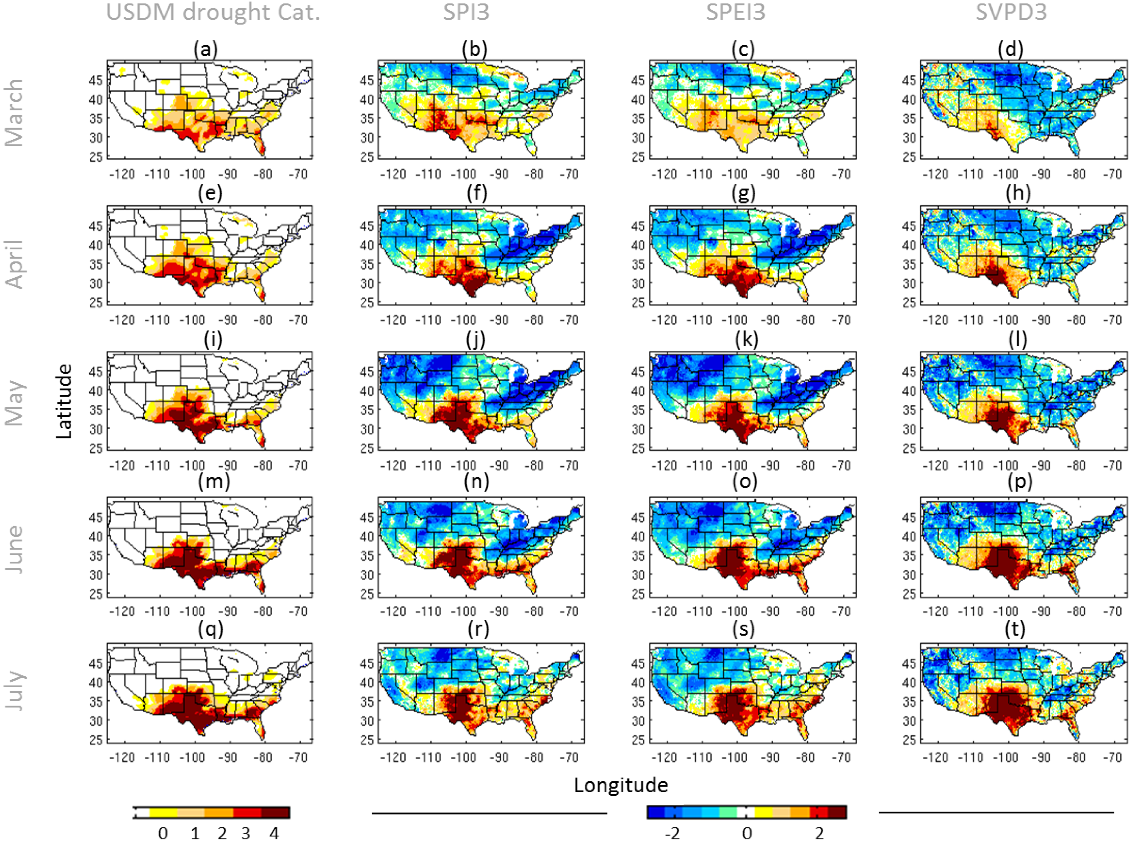
3.2. 2011 Texas Drought

High VPD anomalies can be caused by warm temperature anomalies, below normal humidity, or a combination of both. In the case that temperature is anomalously high and humidity is anomalously low, the VPD is particularly high. Figure 3 shows the development of the 2011 Texas. The drought onset, severity, extent, and the overall development pattern from March through July are generally consistent among USDM and the other indicators. Figure 3, however, shows that there are some discernable differences among the indicators. For example, in April both SPI3 and SPEI3 suggest an exceptional drought in the southernmost part of Texas, while the SVPD3 suggests that the most extreme evapotranspiration demand occurs over the Big Bend region. While USDM only shows small areas of exceptional drought in April, it shows a large coherent area of exceptional drought in May where a large water deficit and anomalously high evapotranspiration demand is identified a month earlier by SPI, SPEI, and especially SVPD3. By June all indicators suggest that almost the entire state of Texas is in exceptional drought. Note that the drought areas identified by USDM and SVPD3 are slightly larger than those identified by SPEI3 and especially SPI3.
Figure 3. Development of 2011 Texas drought based on USDM, SPI3, SPEI3, and SVPD3 plotted from left to right, respectively. From top to bottom the maps correspond to (ad) March, (eh) April, (il) May, (mp) June, and (qt) July of 2011. For SPI3 and SPEI3 the signs are flipped to facilitate the comparison.
Climate 03 00999 g003
Figure 4 further investigates the development of the 2011 Texas drought by dissecting (see Section 2.2.1) the environment VPD anomaly (non-standardized), into its contributing atmospheric temperature and humidity components, and Tmean and Tdmean anomalies. Anomalies are calculated for each month using a 3-month running average (composed of the indicated month and the prior 2 months) relative to the corresponding climatology derived from the entire dataset. In March, the evapotranspiration demand shows positive VPD anomaly in Western and Northwestern Texas and most of New Mexico (Figure 4a). By dissecting the VPD anomaly into the contributing temperature and moisture components, it can be seen that mainly lower than normal moisture (Figure 4c,e) contributes to the observed positive VPD anomaly in March, while the temperature contribution is minimal (Figure 4b,d). In April, a region with high VPD anomaly is evident in Western Texas and Southeastern New Mexico (Figure 4f), which is due to the combined effect of anomalously warm temperatures and anomalously low humidity. As the atmosphere gets warmer and drier the VPD anomaly is enhanced both in coverage and intensity and eventually coincides well with the observed severe drought areas indicated by the drought indices and USDM in Figure 3.
Figure 4. Development of 2011 Texas and southern US drought and the contribution of temperature and humidity in forming high evapotranspiration demand inferred by VPD. From left to right columns represent 3 month (a) VPD anomaly (kPa); (b) temperature contribution to evapotranspiration demand; (c) humidity contribution to 2011 evapotranspirational demand; (d) Tmean anomaly; and (e) Tdmean anomaly. Similar to Figure 3, the maps correspond to (a–e) March, (fj) April, (ko) May, (pt) June, and (uy) July of 2011. Anomalies are calculated based on 3-month average (of a given month and prior 2 months) relative to the corresponding climatology derived from the entire dataset.
Climate 03 00999 g004
It should be noted that, from May to July of 2011, a dry anomaly is observed mainly over western CONUS while warm anomalies are noticeable in the east and southeast regions. The dry and warm anomalies coincide over Texas and amplify the evapotranspiration demand, indicated by very high VPD anomalies exceeding 0.5 kPa (SVPD3 > 2 in Figure 3). Note that the area of extremely high VPD anomaly in July (Figure 4u) is more extensive than the area of extremely low precipitation (Figure 3r). The spatial extent of extreme drought based on SPEI3 appears to fall between that of SPI3 and SVPD3 (Figure 3r–t), as SPEI responds to the higher evapotranspiration demand due to the drier and warmer than normal background state.

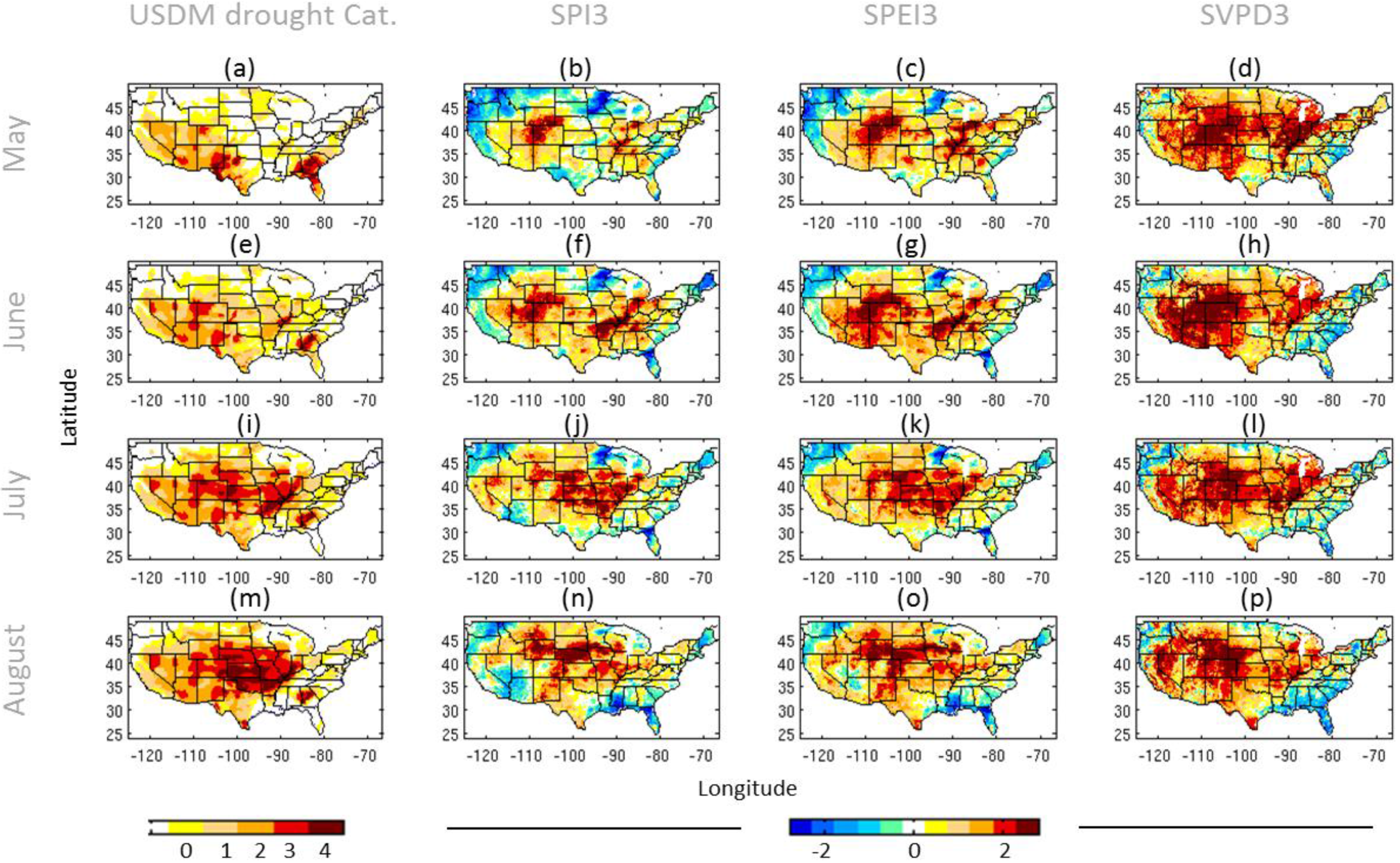
3.3. 2012 Midwest Drought

While all indicators shown in Figure 4 are consistent in capturing the extent and severity of the 2011 Texas drought, this is not the case for the widespread 2012 Midwest US drought. Figure 5 shows the development of the 2012 drought based on USDM, SPI3, SPEI3, and SVPD3 for May, June, July, and August of 2012. Within this period, drought started to develop during May and rapidly reached peak intensity by August. In May the SPI3 and SPEI3 show that 3-month precipitation and precipitation minus evapotranspiration are more than two standardized departures below normal, mainly in the Central Rockies and High Plains, and in portions of the Great Lakes and Mississippi Valley (Figure 5b,c). In June and July, drought areas expanded in both coverage and intensity and by August all indicators, as well as USDM show extensive regions of exceptional drought over the central Great Plains, ranking the event as one of the most severe summertime droughts over the central Great Plains in the last one hundred years. As discussed by Hoerling et al. [52], and references therein, this event was a “flash drought” and its immediate cause was predominantly meteorological. The event was poorly predicted by numerical forecast models, partly due to a lack of strong leading indicators in Pacific Ocean sea surface temperatures [52]. This drought caused major reductions in crop yield, related primarily to water and heat stress. Because SPI3, SPEI3, and SVPD3 all show rapid responses to meteorological conditions, these quantities suggest the development of an exceptional drought before such conditions are apparent in the USDM. Interestingly, SVPD3 in Figure 5 shows extensive regions of exceptionally high VPD (e.g., more than two standardized departures above normal) over the West and Midwest as early as May of 2012, earlier than the other indices. The extensive region of high VPD anomalies was due to a sequence of monthly anomaly patterns in large-scale circulation, such as anticyclonic anomalies at 500 hPa that inhibited precipitation and promoted surface heating through insolation [52].
Unlike the 2011 Texas drought, the location of the exceptionally high SVPD3 in Figure 5 did not fully coincide with the most intense drought regions identified by the other indicators. For example, in May and June of 2012, SVPD3 placed vast areas over the Rocky Mountains and the southwestern US into an exceptionally high VPD (SVPD3 > 2), while SPI3, SPEI3, and USDM showed only about one standardized departure above normal. Had a larger precipitation deficit coincided with the exceptionally high VPD over the Rockies and Southwestern U.S., or the exceptionally high VPD persisted in the Eastern Great Plains, the exceptional drought could be even more severe, more extensive, and developed more rapidly. It should be noted that, besides capturing the background atmospheric state, the VPD anomaly itself is more effective than other drought indicators to predict crop water stress as simulated by a crop model [37]. The development of the 2012 drought coincided with the time for warm season crop sowing in the central US and thus any early warning of future water stress on crops could have been valuable for timely planning and decision making.
Figure 5. Development of 2012 Midwest US drought based on USDM, SPI3, SPEI3, and SVPD3 from left to right, respectively. From top to bottom the maps correspond to (ad) May, (eh) June, (il) July, and (mp) August of 2012. For SPI3 and SPEI3 the signs are flipped to facilitate the comparison.
Climate 03 00999 g005
Figure 6 further investigates the development of the 2012 Midwest US drought by dissecting (see Section 2.2.1) the VPD anomalies into the contributing atmospheric temperature and humidity components and Tmean and Tdmean anomalies. Similar to Figure 4 the anomalies are calculated for each month using 3-month running average. Similar to Figure 5, the maps correspond to May, June, July, and August of 2012. Figure 6 (1st column) shows that both intensity and coverage of an anomalously high VPD (i.e., VPD anomaly greater than 0.5 kPa) rapidly increased from May to August. This means that in addition to the growing water deficit from May to August seen in Figure 5, more water evaporated from the surface than under mean climatic conditions. By dissecting the VPD anomaly into the temperature and humidity components, the development of the background evapotranspiration demand can be better assessed. In May, air temperature in the eastern and central US (and, thus, the contribution of temperature to VPD anomaly there) was extremely high (Figure 6b,d) due to presence of a high-pressure system over the northeast CONUS. However, the atmosphere was anomalously moist in the East and drier than average in the West (Figure 6e). Therefore, the higher than normal VPD in the east was caused by the temperature contribution while both temperature and humidity contributed to the high VPD anomaly in the west.
Figure 6. Development of 2012 Midwest US drought and the contribution of temperature and humidity in forming high evapotranspiration demand inferred by VPD. From left to right columns represent 3 month (a) VPD anomaly (kPa); (b) temperature contribution to evapotranspiration demand; (c) humidity contribution to 2012 evapotranspirational demand; (d) Tmean anomaly; and (e) Tdmean anomaly. Similar to Figure 3, the maps correspond to (a–e) May, (fj) June, (ko) July, and (pt) August of 2011. Anomalies are calculated based on 3-month averages (of a given month and prior 2 months) relative to the corresponding climatology derived from the entire dataset.
Climate 03 00999 g006
As shown in Figure 6, nearly the entire CONUS was anomalously warm during June to August. From June to August the anomalously dry regions in the West expanded eastward and by August more than 60% of the CONUS had an anomalously dry atmosphere (Figure 6, second and fourth columns from left). Clearly, the rapid development and expansion of VPD anomalies in July was due to the combined contribution of anomalously high temperature and low moisture in the western and central US and solely caused by anomalous temperature in the eastern most part of the CONUS. The high VPD anomaly further expanded in August as the drier than normal atmosphere expanded to the east.
The anomalously warm and dry background conditions preceding this drought suggest that indicators based on deficits in precipitation alone do not provide sufficient information for drought monitoring and prediction. An index based solely on precipitation is not sensitive enough to fully capture water stress at any given time. It should be noted that drought areas based on SPEI3 are generally larger and more intense than those obtained from SPI3 (Figure 5). However, calculation of SPEI3, following Vicente-Serrano et al. [12], is based on the Thornthwaite equation, which only requires temperature data. Had we used more complex methods, such as Penman-Monteith, requiring several other variables including humidity, wind speed, and net radiation, the SPEI drought maps may show a more realistic area of net surface water deficit.

3.4. Development of Extreme Drought over the CONUS under Different Atmospheric Temperature and Humidity Background

Knowing that the background state of atmospheric temperature and humidity can significantly influence the level of water stress at the surface, it is reasonable to compare the performance of different drought indices conditioned on the atmospheric state. By investigating how drought indices evolve in different classes of atmospheric states, the effort can help improve prediction skills for both early detection of drought onset and its severity. Here we demonstrate the importance of such information using SPI3 and SPEI3. However the analysis could also be applied to other indices.
First, extreme droughts are identified using the USDM data dating back to 2000. Only droughts identified as D3 or D4 and occurring between May and September are considered. Next, the fraction of grid cells where anomalies in temperature contributes positively to the VPD, and the fraction where moisture contributes positively to the VPD are calculated, concurrent with the drought event (t0). The two fractions are referred to as FCT and FCM respectively. FCM and FCT are calculated for each extreme drought event and plotted in Figure 7. Using k-means clustering [53,54,55] the fractions are grouped into four categories based on their FCT and FCM values. The asterisks in Figure 7 are color coded according to cluster assignment and the black dots represent the cluster centers. Each drought event at time t0 is assigned to one of the four clusters (shown Figure 7) and the time series of the domain average of SPI3 and SPEI3 for all four clusters from five months prior (t-5) to t0 are plotted in Figure 8.
Figure 7. Fraction of positively contributing temperature (FCT; X-axis) and the fraction of positively contributing moisture (FCM; Y-axis) to VPD under extreme and exceptional drought categories (USDM D3 and D4). The Kmeans clustering method is used for classifying the fractions into four groups shown in different colors. The black dots show the centroid of each of the four clusters.
Climate 03 00999 g007
In group 1 (Figure 7), both temperature and humidity contribute significantly to evapotranspiration demand (e.g., FCM > 0.7 and FCT > 0.7 in Figure 8a). Given the extensive hot and dry conditions, both SPI3 and SPEI3 show severe drought (e.g., standardized index less than −1.2) as far as five months before the USDM reaches or exceeds Category D3. Moving towards to drought becomes more severe as suggested by USDM (Figure 8i), but only SPEI3 appears to capture the increase in severity of drought conditions while SPI3 stays constant or increases toward zero (Figure 8e). This suggests that for group 1, precipitation alone is not sufficient to fully capture drought development. For group 2, which features an environment with temperature contributing much more extensively (e.g., FCT > 0.8) than humidity to VPD (Figure 7 and Figure 8b), SPEI3 suggests a more severe drought than SPI3 (Figure 8f) at each time step. So, for a given deviation from normal (shown on the Y-axis) SPEI3 captures the deviation (or the severity of drought) about a month earlier than SPI3. For group 3 (Figure 7 and Figure 8c), in which temperature shows a greater contribution than humidity to VPD (but not as much as that in group 2), SPI3 and SPEI3 are nearly identical throughout the five-month period. Unlike the other three groups, moisture contributes more than temperature to evapotranspiration demand for group 4 (Figure 7 and Figure 8d). Figure 8h shows that in this group SPI3 captures severe drought conditions earlier than SPEI3. Further examination shows that group 4 occurs more frequently during cold season and near coastal regions suggesting that in such conditions SPI can be more effective than SPEI for early detection of drought. The above analysis confirms that monitoring the background state of atmospheric temperature and humidity can more efficiently capture the timing and intensity of drought than precipitation alone.
Figure 8. The cluster averages of the time series plotted separately for each group identified in Figure 7. From left to light the columns represent groups 1 to 4, respectively. The top row (ad) shows the fraction of positively contributing temperature (FCT) and moisture (FCM) to VPD, the middle row (eh) shows the standardized indices (here, SPI3 and SPEI3) as drought reaches an extreme or exceptional USDM categories at time step 0 (to in text), and the bottom row (il) represents USDM drought category.
Climate 03 00999 g008

4. Concluding Remarks

The combined effects of atmospheric temperature and moisture in the development of warm season drought is examined in more than a century of high-resolution PRISM temperature, dewpoint temperature, and precipitation data, and a decade of U.S. Drought Monitor (USDM) data over the CONUS. The analysis of the historical data shows that the fraction of CONUS area experiencing extremely high temperature and evapotranspiration demand has been increasing during last few decades, while a similar feature has not been observed for precipitation. This implies that aridity over land can increase even if precipitation remains the same or increases, as a warmer climate will increase evaporative demand through hotter or drier atmospheric states. Vapor pressure deficit (VPD) is identified as a robust index to determine the background atmospheric state, in relation to temperature and humidity, and evapotranspiration demand. VPD anomalies are partitioned into atmospheric temperature and moisture components to better assess different drought events. The partitioning of VPD is performed by replacing one variable at a time with its climatological mean in the VPD equation (Section 2.2.1).
Two exceptional events, the 2011 Texas and the 2012 Midwest droughts, are selected to examine how the combination of atmospheric temperature and humidity together with precipitation deficit form exceptional summer droughts. It is observed that the two cases had different atmospheric background states during their development. While lower than normal moisture contributed mainly to the observed high evapotranspiration demand during the early months of development of the 2011 Texas drought, eventually the combination of both hot and dry anomalies rapidly formed an exceptionally high VPD over the most of Texas. The anomalously high VPD in this region coincided with the exceptional drought identified by SPI and USDM there. However, for the widespread 2012 drought, the region of the anomalously high VPD was much more extensive than that identified as exceptional droughts by SPI and USDM. The first signal of an extreme drought in the Midwest was evident in VPD anomaly maps about two month earlier than with other indices. The rapid amplification and expansion of VPD anomalies in July was due to a combination of anomalously high temperature and low moisture in the Western and Central US, while temperature was the main contributing factor over eastern CONUS. Clearly, in such hot and dry atmospheric conditions, considering only precipitation deficit for drought monitoring and prediction is insufficient because it cannot capture the level of water stress. This is critical in a warming climate as the background atmosphere also becomes drier [32]. By combining temperature and humidity into a single quantity, VPD is found as a robust tool to monitor the background atmospheric state preceding and during a drought event with potential to help predict drought onset and intently in advance.
We further investigate how drought indices (e.g., SPEI and SPI) perform as droughts develop in a given atmospheric state. Characterization of droughts based on their atmospheric state in their early stage of development can help improve predicting how they will evolve in future. This was performed by identifying the extreme and exceptional warm season droughts using the entire USDM record, assigning each to a class of atmospheric state, and assessing the path that drought indices SPI and SPEI in each class took to reach to the extreme or exceptional drought observed by USDM. The analysis suggests that monitoring the background atmospheric state is invaluable to give insights about the timing and intensity of drought suggested by each drought indicator. This can potentially advance the early detection of drought and making timely decisions.
The analysis performed here is potentially extendable to global scale by using both satellite observations and reanalysis products. The Atmospheric Infrared Sounder (AIRS) is carried on the Aqua satellite, part of the NASA Earth Observing System [56]. Since 2002, AIRS has provided global high quality atmospheric temperature and moisture data. With the launch of IASI on MetOp in 2006 and the Cross-track Infrared Sounder (CrIS) on the Suomi National Polar-orbiting Partnership (NPP) in 2012, and a suite of operational microwave sounders, additional sampling of atmospheric temperature and moisture are available. Given the importance of the atmospheric background in the development and formation of drought, creating a consistent global data record from a variety of sources is an important logical step, which is currently underway by the authors.

Acknowledgments

The research described in this paper was carried out at the Jet Propulsion Laboratory, California Institute of Technology, under a contract with the National Aeronautics and Space Administration. Government sponsorship is acknowledged. We are thankful to Calvin Poulsen and Mark Svoboda of National Drought Mitigation Center for their support and collaboration.

Author Contributions

All authors have contributed to the idea and hypothesis development, method development, data processing, analyses, interpretation of the results, and writing the manuscript.

Conflicts of Interest

The authors declare no conflict of interest.

References

  1. Mueller, B.; Seneviratne, S.I. Hot days induced by precipitation deficits at the global scale. Proc. Natl. Acad. Sci. USA 2012, 109, 12398–12403. [Google Scholar] [CrossRef] [PubMed]
  2. Fischer, E.M.; Seneviratne, S.I.; Vidale, P.L.; Lüthi, D.; Schär, C. Soil moisture-atmosphere interactions during the 2003 European summer heat wave. J. Clim. 2007, 20, 5081–5099. [Google Scholar] [CrossRef]
  3. Loikith, P.C.; Broccoli, A.J. The influence of recurrent modes of climate variability on the occurrence of winter and summer extreme temperatures over North America. J. Clim. 2014, 27, 1600–1618. [Google Scholar] [CrossRef]
  4. Zhou, B.; Xu, Y.; Wu, J.; Dong, S.; Shi, Y. Changes in temperature and precipitation extreme indices over china: Analysis of a high-resolution grid dataset. Int. J. Climatol. 2015. [Google Scholar] [CrossRef]
  5. Below, R.; Grover-Kopec, E.; Dilley, M. Documenting drought-related disasters: A global reassessment. J. Environ. Dev. 2007, 16, 328–344. [Google Scholar] [CrossRef]
  6. Smith, A.; Katz, R. Us billion-dollar weather and climate disasters: Data sources, trends, accuracy and biases. Nat. Hazards 2013, 67, 387–410. [Google Scholar] [CrossRef]
  7. Haile, M. Weather patterns, food security and humanitarian response in sub-Saharan Africa. Philos. Trans. R. Soc. B Biol. Sci. 2005, 360, 2169–2182. [Google Scholar] [CrossRef] [PubMed]
  8. Changnon, S.A.; Easterling, W.E. Measuring drought impacts: The Illinois case1. JAWRA J. Am. Water Resour. Assoc. 1989, 25, 27–42. [Google Scholar] [CrossRef]
  9. Eltahir, E.A.B.; Yeh, P.J.F. On the asymmetric response of aquifer water level to floods and droughts in illinois. Water Resour. Res. 1999, 35, 1199–1217. [Google Scholar] [CrossRef]
  10. Pandey, R.P.; Ramasastri, K.S. Relationship between the common climatic parameters and average drought frequency. Hydrol. Process. 2001, 15, 1019–1032. [Google Scholar] [CrossRef]
  11. Mishra, A.K.; Singh, V.P. A review of drought concepts. J. Hydrol. 2010, 391, 202–216. [Google Scholar] [CrossRef]
  12. Vicente-Serrano, S.M.; Begueria, S.; Lopez-Moreno, J.I. A multiscalar drought index sensitive to global warming: The standardized precipitation evapotranspiration index. J. Clim. 2010, 23, 1696–1718. [Google Scholar] [CrossRef]
  13. McKee, T.B.; Doesken, N.J.; Kleist, J. The relationship of drought frequency and duration to time scales. In Proceedings of the Eighth Conference on Applied Climatology, Anaheim, CA, USA, 17–22 January 1993; pp. 179–184.
  14. Quan, X.-W.; Hoerling, M.P.; Lyon, B.; Kumar, A.; Bell, M.A.; Tippett, M.K.; Wang, H. Prospects for dynamical prediction of meteorological drought. J. Appl. Meteorol. Climatol. 2012, 51, 1238–1252. [Google Scholar] [CrossRef]
  15. Lyon, B.; Bell, M.A.; Tippett, M.K.; Kumar, A.; Hoerling, M.P.; Quan, X.-W.; Wang, H. Baseline probabilities for the seasonal prediction of meteorological drought. J. Appl. Meteorol. Climatol. 2012, 51, 1222–1237. [Google Scholar] [CrossRef]
  16. Yuan, X.; Wood, E.F. Multimodel seasonal forecasting of global drought onset. Geophys. Res. Lett. 2013, 40, 4900–4905. [Google Scholar] [CrossRef]
  17. Behrangi, A.; Nguyen, H.; Granger, S. Probabilistic seasonal prediction of meteorological drought using the bootstrap and multivariate information. J. Appl. Meteorol. Climatol. 2015, 54, 1510–1522. [Google Scholar] [CrossRef]
  18. Ganguli, P.; Reddy, M.J. Evaluation of trends and multivariate frequency analysis of droughts in three meteorological subdivisions of western india. Int. J. Climatol. 2014, 34, 911–928. [Google Scholar] [CrossRef]
  19. Abramopoulos, F.; Rosenzweig, C.; Choudhury, B. Improved ground hydrology calculations for global climate models (GCMS): Soil water movement and evapotranspiration. J. Clim. 1988, 1, 921–941. [Google Scholar] [CrossRef]
  20. Dai, A.; Trenberth, K.E.; Qian, T. A global dataset of palmer drought severity index for 1870–2002: Relationship with soil moisture and effects of surface warming. J. Hydrometeorol. 2004, 5, 1117–1130. [Google Scholar] [CrossRef]
  21. Nicholls, N. The changing nature of australian droughts. Clim. Chang. 2004, 63, 323–336. [Google Scholar] [CrossRef]
  22. Van Dijk, A.I.J.M.; Beck, H.E.; Crosbie, R.S.; de Jeu, R.A.M.; Liu, Y.Y.; Podger, G.M.; Timbal, B.; Viney, N.R. The millennium drought in southeast Australia (2001–2009): Natural and human causes and implications for water resources, ecosystems, economy, and society. Water Resour. Res. 2013, 49, 1040–1057. [Google Scholar] [CrossRef]
  23. Lewis, S.C.; Karoly, D.J. Anthropogenic contributions to australia’s record summer temperatures of 2013. Geophys. Res. Lett. 2013, 40, 3705–3709. [Google Scholar] [CrossRef]
  24. Vicente-Serrano, S.M.; Beguería, S.; Lorenzo-Lacruz, J.; Camarero, J.s.J.; López-Moreno, J.I.; Azorin-Molina, C.; Revuelto, J.S.; Morán-Tejeda, E.; Sanchez-Lorenzo, A. Performance of drought indices for ecological, agricultural, and hydrological applications. Earth Interact. 2012, 16, 1–27. [Google Scholar] [CrossRef]
  25. Wang, Q.; Shi, P.; Lei, T.; Geng, G.; Liu, J.; Mo, X.; Li, X.; Zhou, H.; Wu, J. The alleviating trend of drought in the Huang-Huai-Hai plain of China based on the daily SPEI. Int. J. Climatol. 2015. [Google Scholar] [CrossRef]
  26. Feng, S.; Fu, Q. Expansion of global drylands under a warming climate. Atmos. Chem. Phys. 2013, 13, 10081–10094. [Google Scholar] [CrossRef]
  27. Dai, A. Increasing drought under global warming in observations and models. Nat. Clim. Chang. 2013, 3, 52–58. [Google Scholar] [CrossRef]
  28. Dai, A. Recent climatology, variability, and trends in global surface humidity. J. Clim. 2006, 19, 3589–3606. [Google Scholar] [CrossRef]
  29. Joshi, M.; Gregory, J. Dependence of the land-sea contrast in surface climate response on the nature of the forcing. Geophys. Res. Lett. 2008, 35, L24802. [Google Scholar] [CrossRef]
  30. Simelton, E. Coping with Drought Risk in Agriculture and Water Supply Systems: Drought Management and Policy Development in the Mediterranean (Advances in Natural and Technological Hazards Research); Iglesias, A., Garrote, L., Cancelliere, A., Cubillo, F., Wilhite, D., Eds.; Springer: Berlin, Germany, 2009. [Google Scholar]
  31. Byrne, M.P.; O’ Gorman, P.A. Land-ocean warming contrast over a wide range of climates: Convective quasi-equilibrium theory and idealized simulations. J. Clim. 2013, 26, 4000–4016. [Google Scholar] [CrossRef]
  32. Sherwood, S.; Fu, Q. A drier future? Science 2014, 343, 737–739. [Google Scholar] [CrossRef] [PubMed]
  33. Stephens, G.L.; Ellis, T.D. Controls of global-mean precipitation increases in global warming gcm experiments. J. Clim. 2008, 21, 6141–6155. [Google Scholar] [CrossRef]
  34. Cook, B.; Smerdon, J.; Seager, R.; Coats, S. Global warming and 21st century drying. Clim. Dyn. 2014, 43, 2607–2627. [Google Scholar] [CrossRef]
  35. Seager, R.; Hooks, A.; Williams, A.P.; Cook, B.; Nakamura, J.; Henderson, N. Climatology, variability, and trends in the U.S. Vapor pressure deficit, an important fire-related meteorological quantity. J. Appl. Meteorol. Climatol. 2015, 54, 1121–1141. [Google Scholar] [CrossRef]
  36. Williams, A.P.; Seager, R.; Berkelhammer, M.; Macalady, A.K.; Crimmins, M.A.; Swetnam, T.W.; Trugman, A.T.; Buenning, N.; Hryniw, N.; McDowell, N.G.; et al. Causes and implications of extreme atmospheric moisture demand during the record-breaking 2011 wildfire season in the southwestern united states. J. Appl. Meteorol. Climatol. 2014, 53, 2671–2684. [Google Scholar] [CrossRef]
  37. Lobell, D.B.; Roberts, M.J.; Schlenker, W.; Braun, N.; Little, B.B.; Rejesus, R.M.; Hammer, G.L. Greater sensitivity to drought accompanies maize yield increase in the U.S. Midwest. Science 2014, 344, 516–519. [Google Scholar] [CrossRef] [PubMed]
  38. Daly, C.; Neilson, R.P.; Phillips, D.L. A statistical-topographic model for mapping climatological precipitation over mountainous terrain. J. Appl. Meteorol. 1994, 33, 140–158. [Google Scholar] [CrossRef]
  39. Daly, C.; Gibson, W.P.; Taylor, G.H.; Johnson, G.L.; Pasteris, P. A knowledge-based approach to the statistical mapping of climate. Clim. Res. 2002, 22, 99–113. [Google Scholar] [CrossRef]
  40. Svoboda, M.; LeComte, D.; Hayes, M.; Heim, R.; Gleason, K.; Angel, J.; Rippey, B.; Tinker, R.; Palecki, M.; Stooksbury, D.; et al. The drought monitor. Bull. Am. Meteorol. Soc. 2002, 83, 1181–1190. [Google Scholar]
  41. Anderson, M.C.; Hain, C.; Otkin, J.; Zhan, X.W.; Mo, K.; Svoboda, M.; Wardlow, B.; Pimstein, A. An intercomparison of drought indicators based on thermal remote sensing and NLDAS-2 simulations with us drought monitor classifications. J. Hydrometeorol. 2013, 14, 1035–1056. [Google Scholar] [CrossRef]
  42. Wu, H.; Svoboda, M.D.; Hayes, M.J.; Wilhite, D.A.; Wen, F. Appropriate application of the standardized precipitation index in arid locations and dry seasons. Int. J. Climatol. 2007, 27, 65–79. [Google Scholar] [CrossRef]
  43. Shukla, S.; Wood, A.W. Use of a standardized runoff index for characterizing hydrologic drought. Geophys. Res. Lett. 2008, 35. [Google Scholar] [CrossRef]
  44. Thornthwaite, C.W. An approach toward a rational classification of climate. Geogr. Rev. 1948, 38, 55–94. [Google Scholar] [CrossRef]
  45. Weiss, J.L.; Betancourt, J.L.; Overpeck, J.T. Climatic limits on foliar growth during major droughts in the southwestern USA. J. Geophys. Res. Biogeosci. 2012, 117. [Google Scholar] [CrossRef]
  46. Weiss, J.L.; Overpeck, J.T.; Cole, J.E. Warmer led to drier: Dissecting the 2011 drought in the southern U.S. Southwest Clim. Outlook 2012, 11, 3–4. [Google Scholar]
  47. Edwards, E.C.; McKee, T.B. Characteristics of 20th Century Drought in the United States at Multiple Time Scales; Climatology Report 97–2; Department of Atmospheric Science, Colorado State University: Fort Collins, CO, USA, 1997. [Google Scholar]
  48. Andreadis, K.M.; Clark, E.A.; Wood, A.W.; Hamlet, A.F.; Lettenmaier, D.P. Twentieth-century drought in the conterminous United States. J. Hydrometeorol. 2005, 6, 985–1001. [Google Scholar] [CrossRef]
  49. Wang, A.; Bohn, T.J.; Mahanama, S.P.; Koster, R.D.; Lettenmaier, D.P. Multimodel ensemble reconstruction of drought over the continental united states. J. Clim. 2009, 22, 2694–2712. [Google Scholar] [CrossRef]
  50. Hao, Z.C.; AghaKouchak, A. A nonparametric multivariate multi-index drought monitoring framework. J. Hydrometeorol. 2014, 15, 89–101. [Google Scholar] [CrossRef]
  51. Gringorten, I.I. A plotting rule for extreme probability paper. J. Geophys. Res. 1963, 68, 813–814. [Google Scholar] [CrossRef]
  52. Hoerling, M.; Eischeid, J.; Kumar, A.; Leung, R.; Mariotti, A.; Mo, K.; Schubert, S.; Seager, R. Causes and predictability of the 2012 Great Plains drought. Bull. Am. Meteorol. Soc. 2014, 95, 269–282. [Google Scholar] [CrossRef]
  53. Duda, R.; Hart, P. Pattern Classification and Scene Analysis; John Wiley & Sons: New York, NY, USA, 1973. [Google Scholar]
  54. Everitt, B.S. Cluster Analysis, 3rd ed.; Halsted Press: New York, NY, USA, 1993. [Google Scholar]
  55. Qiu, D.; Tamhane, A.C. A comparative study of the k-means algorithm and the normal mixture model for clustering: Univariate case. J. Stat. Plan. Inference 2007, 137, 3722–3740. [Google Scholar] [CrossRef]
  56. Aumann, H.H.; Chahine, M.T.; Gautier, C.; Goldberg, M.D.; McMillin, L.M.; Revercomb, H.; Kalnay, E.; Rosenkranz, P.W.; Smith, W.L.; Staelin, D.H.; et al. AIRS/AMSU/HSB on the aqua mission: Design, science objectives, data products, and processing systems. IEEE Trans. Geosci. Remote Sens. 2003, 41, 253–264. [Google Scholar] [CrossRef]

