The Effects of Great Plains Irrigation on the Surface Energy Balance, Regional Circulation, and Precipitation

Abstract
:1. Introduction
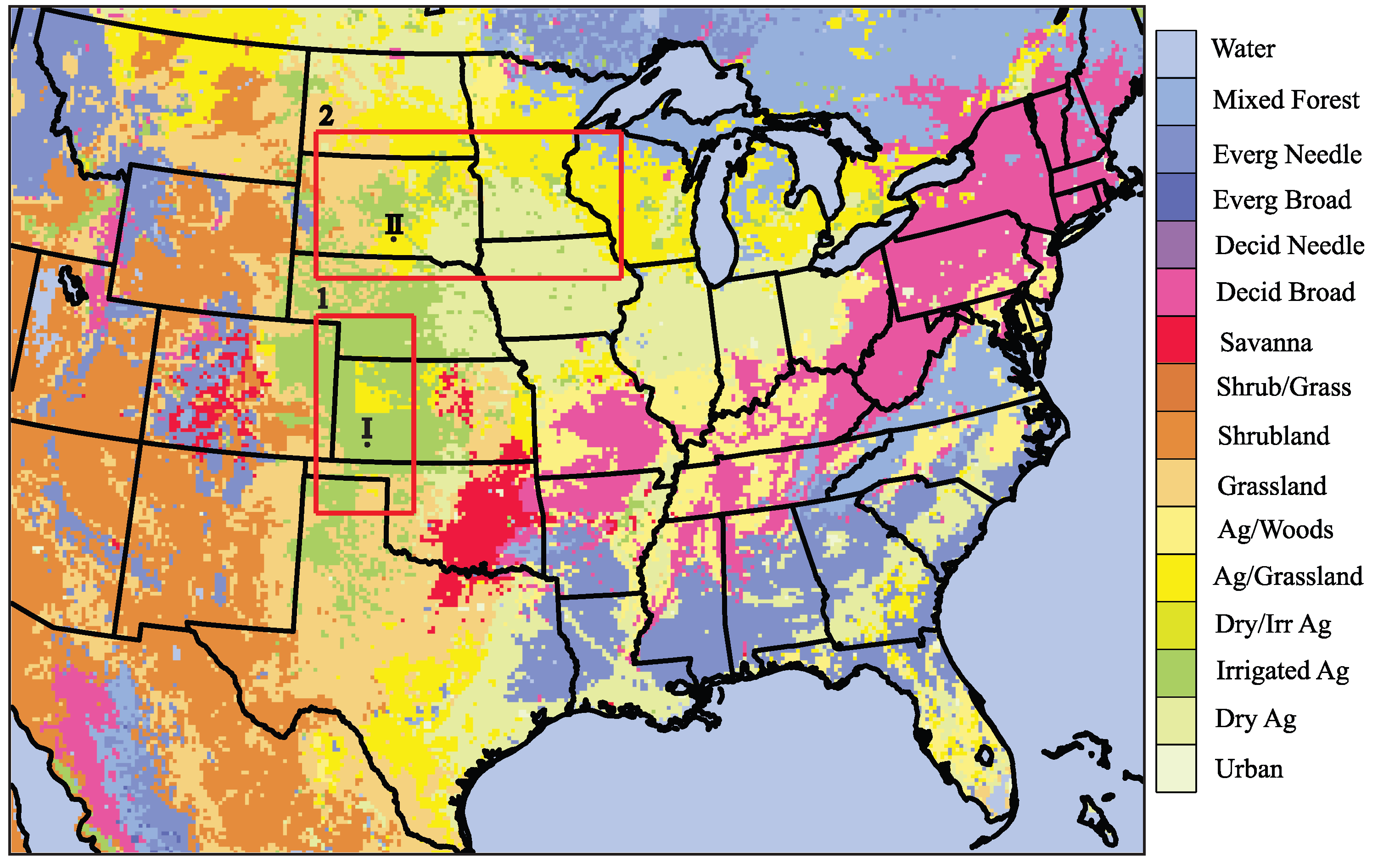
2. Methodology
3. Simulation Results
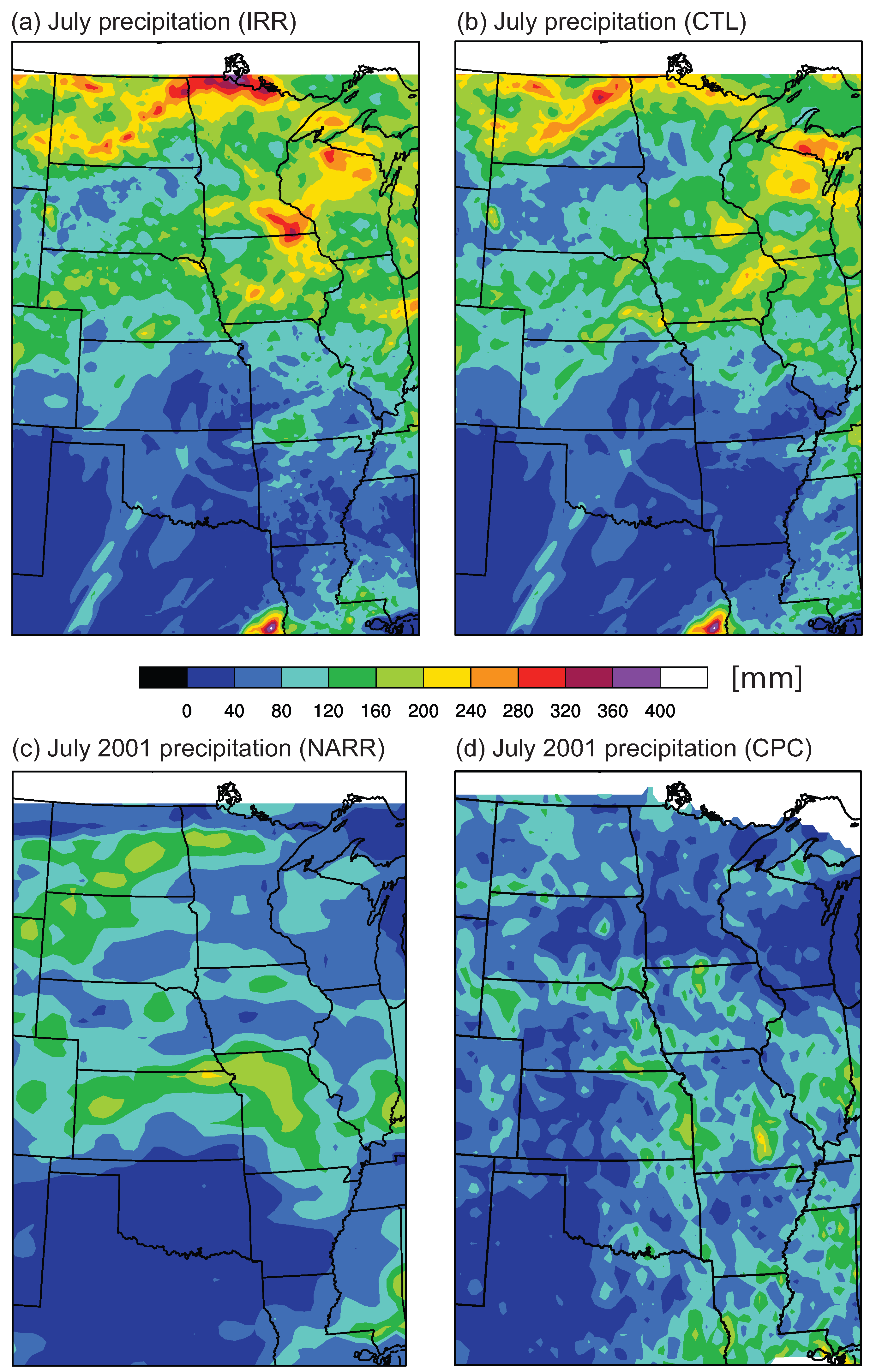
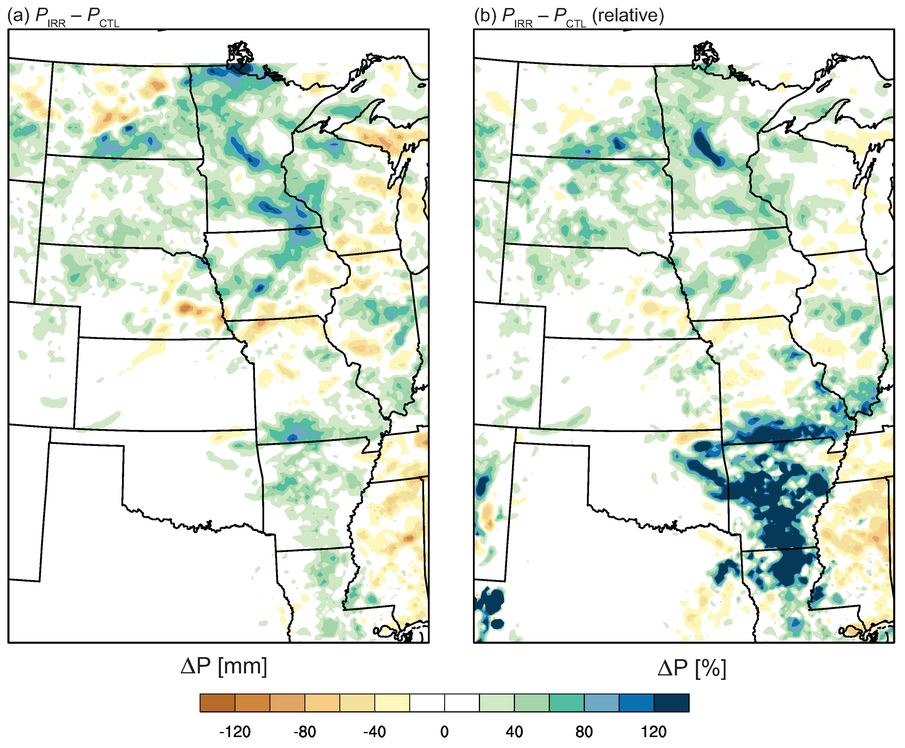
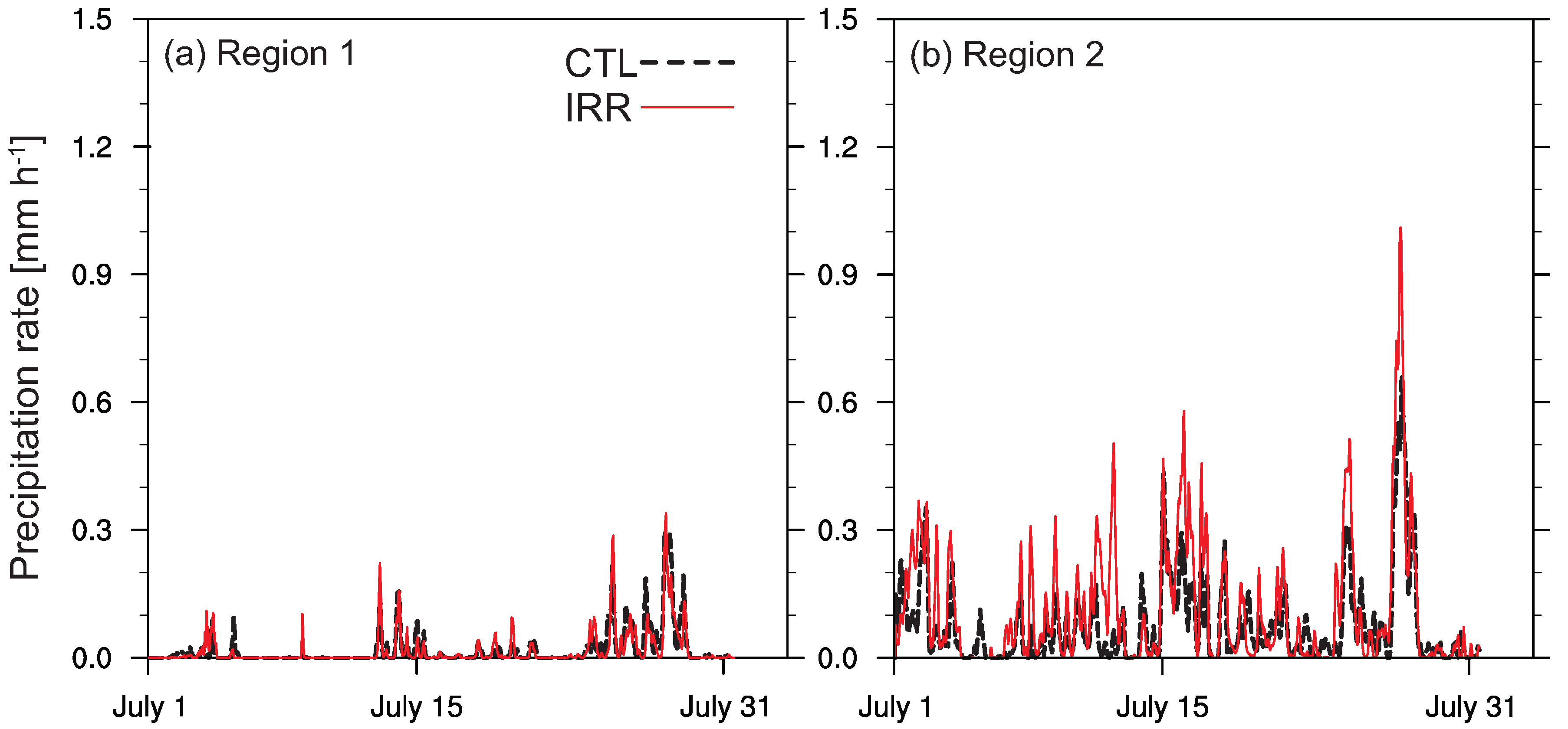
3.1. Precipitation

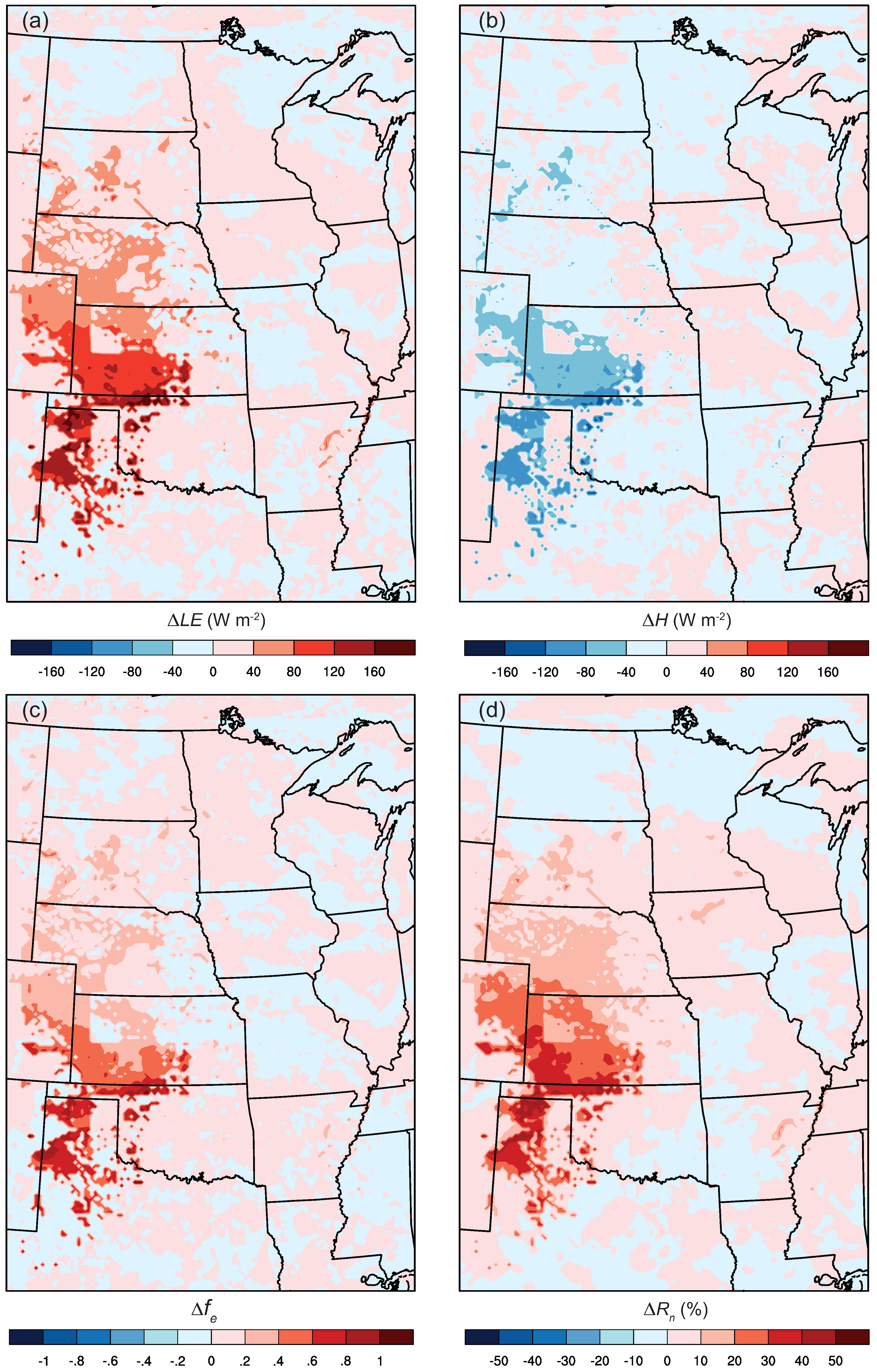
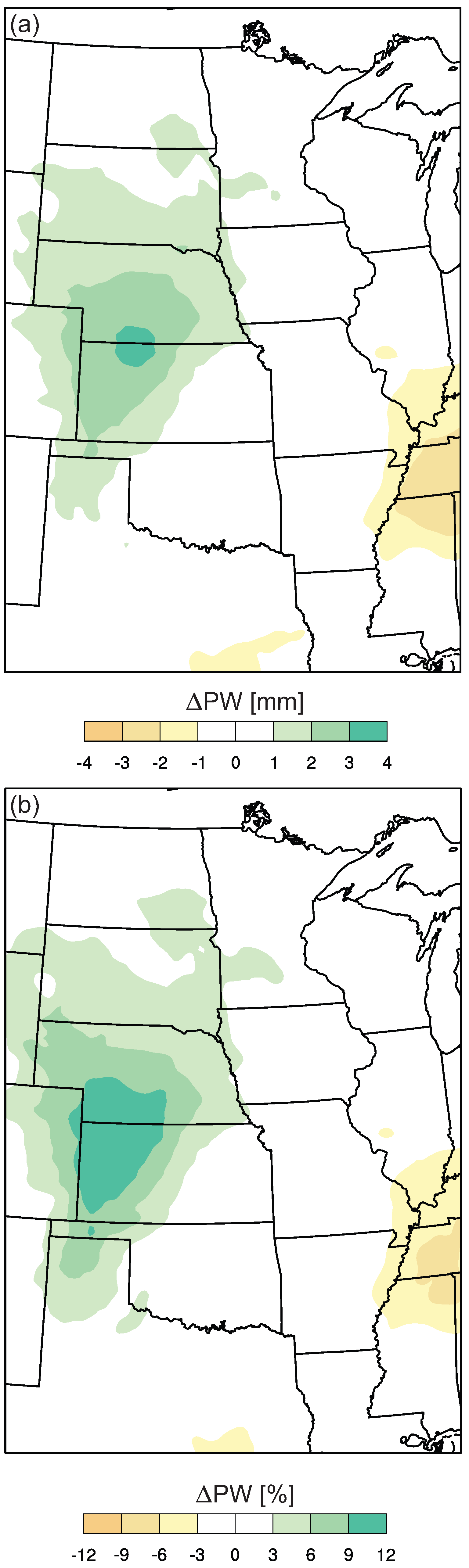
3.2. Surface Radiation Budget


| Variable | Region 1 | Variable | Region 2 | ||||
|---|---|---|---|---|---|---|---|
| IRR | CTL | Diff. (%) | IRR | CTL | Diff. (%) | ||
| T (K) | 302.3 | 307.0 | –4.7 (–1.5) | T (K) | 299.8 | 300.8 | –1.0 (–0.3) |
| H (W·m) | 20.6 | 57.7 | –37.1 (–64.3) | H (W·m) | 34.2 | 39.2 | –5.0 (–12.8) |
| (W·m) | 142.9 | 75.5 | 67.4 (89.3) | (W·m) | 112.1 | 101.6 | 10.5 (10.3) |
| G (W·m) | 6.8 | 7.3 | –0.5 (–6.8) | G (W·m) | 8.1 | 8.6 | –0.5 (–5.8) |
| LW (W·m) | 458.8 | 488.9 | –30.1 (–6.2) | LW (W·m) | 433.6 | 439.7 | –6.1 (–1.4) |
| LW (W·m) | 359.9 | 364.0 | –4.1 (–1.1) | LW (W·m) | 353.4 | 352.5 | 0.9 (0.3) |
| LW (W·m) | –98.9 | –124.9 | 26.0 (20.8) | LW (W·m) | –80.2 | –87.2 | 7.0 (8.0) |
| SW (W·m) | 268.5 | 264.2 | 4.3 (1.6) | SW (W·m) | 234.5 | 236.3 | –1.8 (–0.7) |
| (W·m) | 169.6 | 139.3 | 30.3 (21.8) | (W·m) | 154.2 | 149.0 | 5.2 (3.5) |

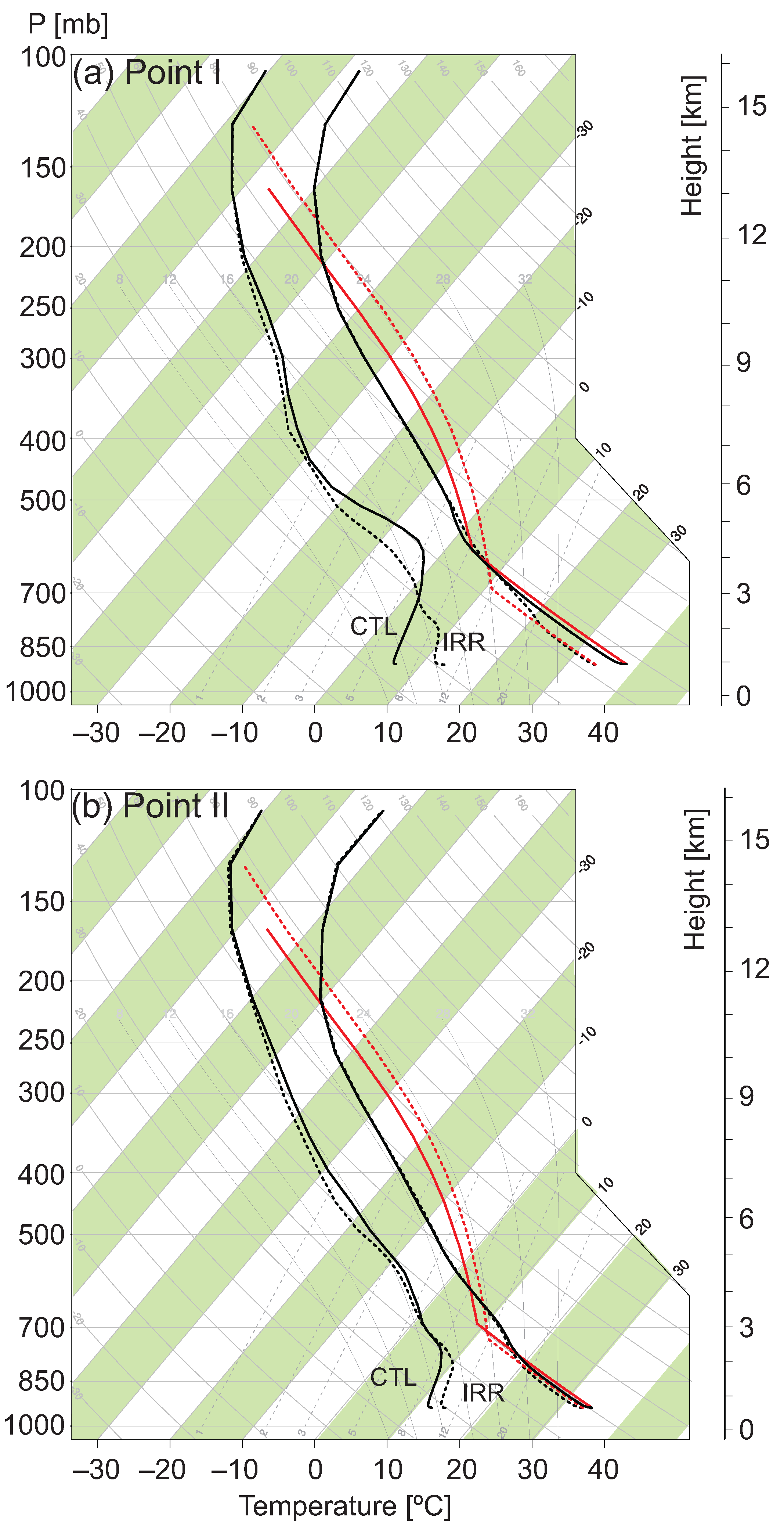
3.3. Vertical Thermodynamic Structure
| Variable | Region 1 | Variable | Region 2 | ||||
|---|---|---|---|---|---|---|---|
| IRR | CTL | Diff. (%) | IRR | CTL | Diff. (%) | ||
| (K) | 301.9 | 306.6 | –4.7 (–1.5) | T (K) | 299.4 | 300.4 | –1.0 (–0.3) |
| W (mm) | 27.6 | 25.5 | 2.1 (8.2) | W (mm) | 31.7 | 30.9 | 0.9 (2.8) |
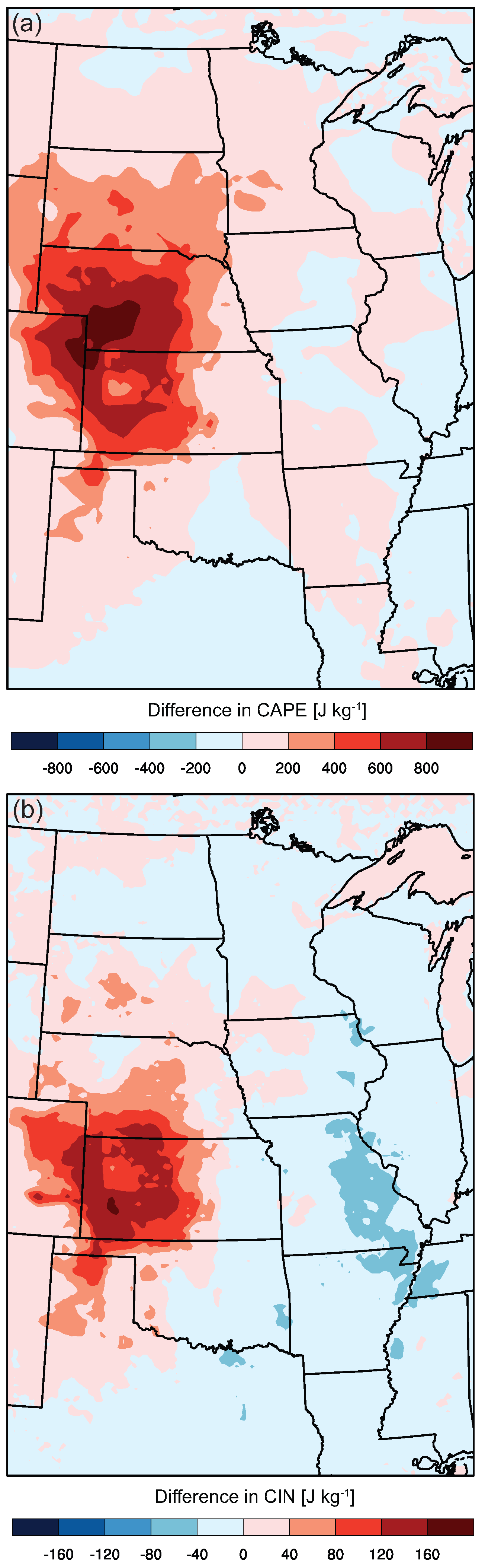
| CAPE (J·kg) | 654.7 | 209.8 | 444.8 (212.0) | CAPE (J·kg) | 791.8 | 577.5 | 214.3 (37.1) |
| CIN (J·kg) | 160.7 | 74.9 | 85.8 (114.5) | CIN (J·kg) | 103.8 | 122.3 | –18.5 (–15.1) |
| P (mm) | 12.5 | 13.6 | –1.1 (–7.9) | P (mm) | 82.7 | 56.9 | 25.9 (45.5) |
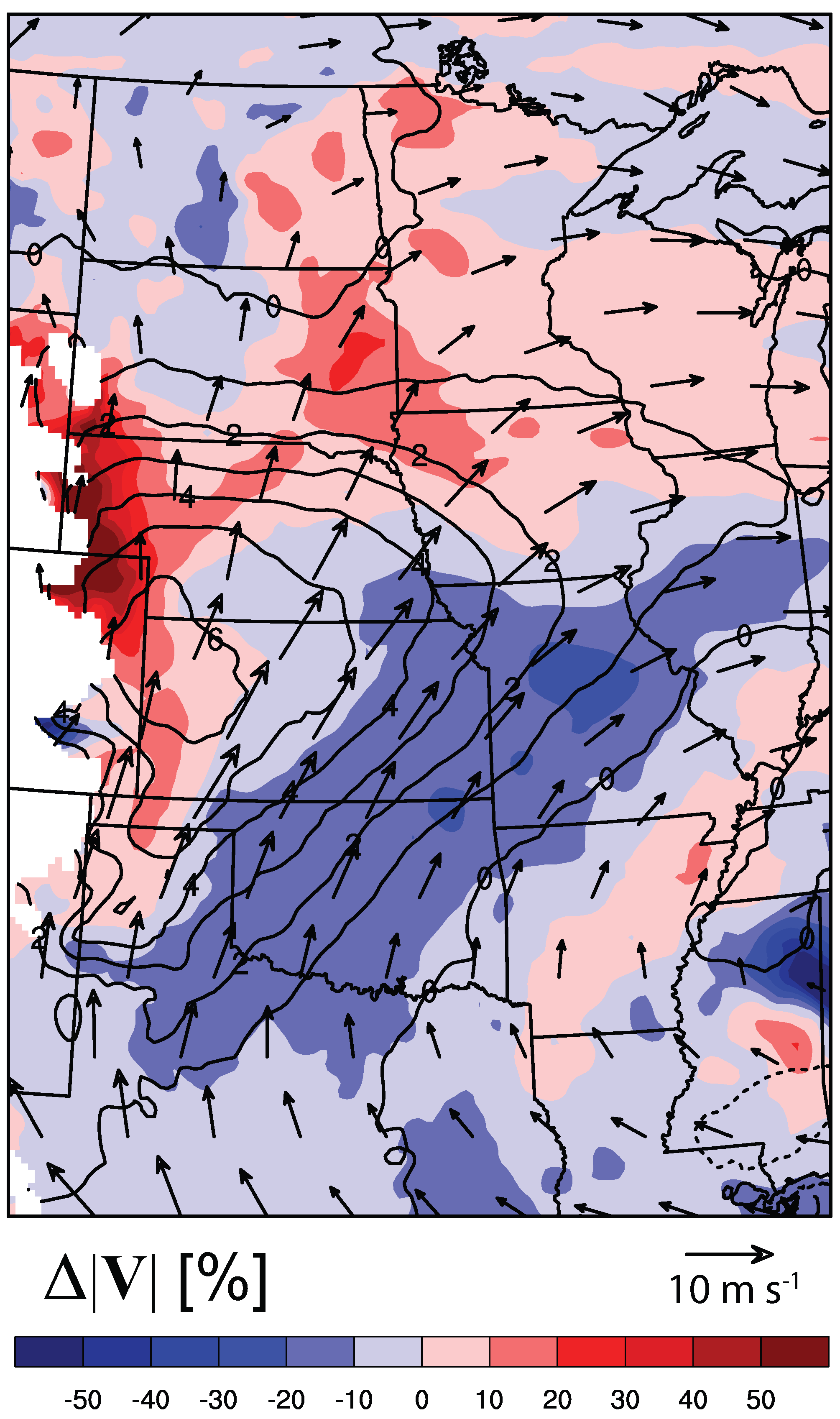
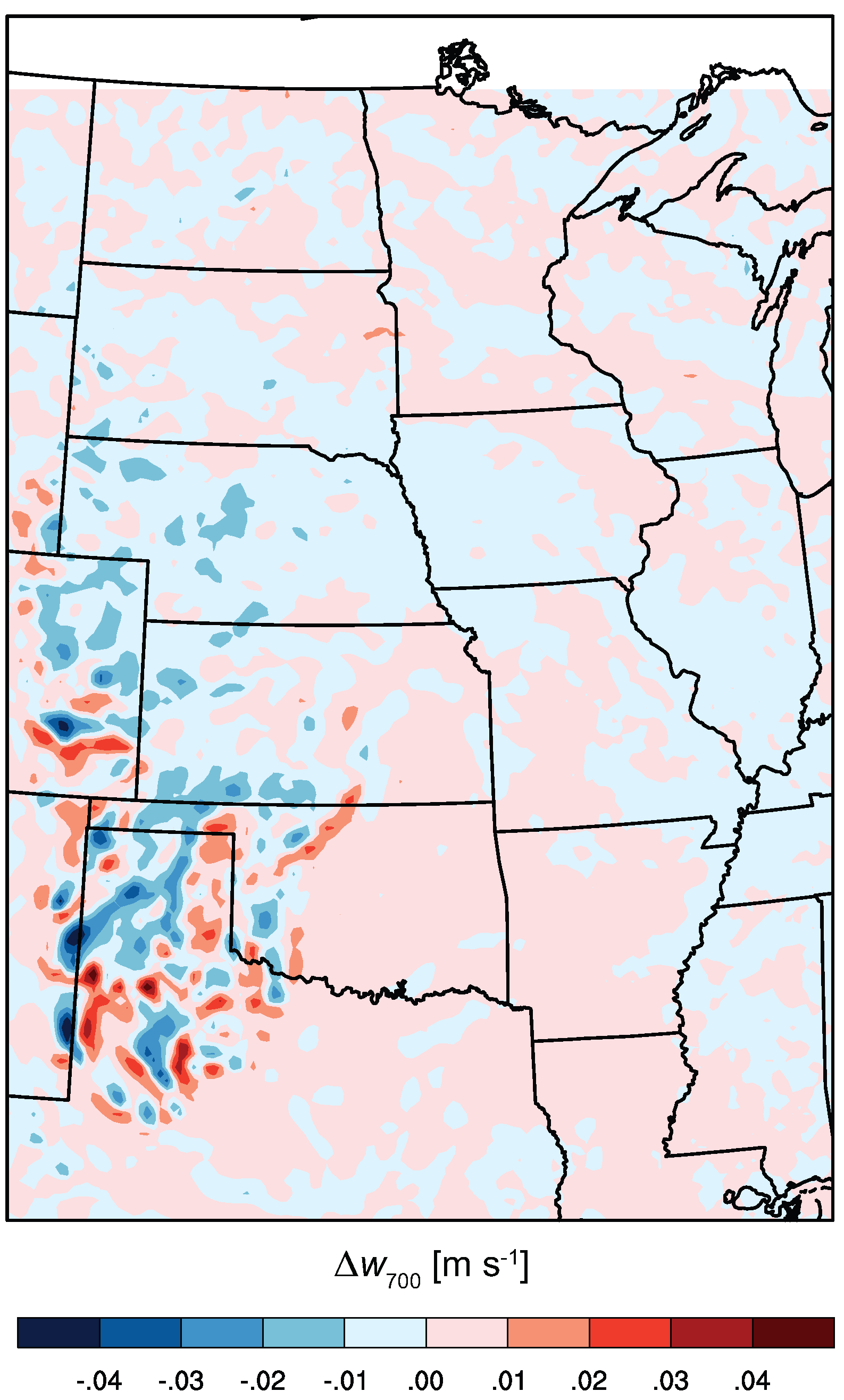
3.4. Lower-Atmospheric Flow


3.5. Differences in Precipitation Behavior
4. Discussion and Conclusions
Acknowledgments
Author Contributions
Conflicts of Interest
References
- Hansen, J.; Sato, M.; Ruedy, R.; Nazarenko, L.; Lacis, A.; Schmidt, G.; Russell, G.; Aleinov, I.; Bauer, M.; Bauer, S.; et al. Efficacy of climate forcings. J. Geophys. Res. Atmos. (1984–2012) 2005, 110. [Google Scholar] [CrossRef]
- Pielke, R.A. Influence of the spatial distribution of vegetation and soils on the prediction of cumulus convective rainfall. Rev. Geophys. 2001, 39, 151–177. [Google Scholar] [CrossRef]
- Brunsell, N.A.; Jones, A.R.; Jackson, T.; Feddema, J. Seasonal trends in air temperature and precipitation in IPCC AR4 GCM output for Kansas, USA: Evaluation and implications. Int. J. Climatol. 2010, 30, 1178–1193. [Google Scholar] [CrossRef]
- Koster, R.D.; Dirmeyer, P.A.; Guo, Z.; Bonan, G.; Chan, E.; Cox, P.; Gordon, C.; Kanae, S.; Kowalczyk, E.; Lawrence, D.; et al. Regions of strong coupling between soil moisture and precipitation. Science 2004, 305, 1138–1140. [Google Scholar] [CrossRef] [PubMed]
- Brunsell, N. Characterization of land-surface precipitation feedback regimes with remote sensing. Remote Sens. Environ. 2006, 100, 200–211. [Google Scholar] [CrossRef]
- Jones, A.; Brunsell, N. A scaling analysis of soil moisture–precipitation interactions in a regional climate model. Theor. Appl. Climatol. 2009, 98, 221–235. [Google Scholar] [CrossRef]
- Jones, A.R.; Brunsell, N.A. Energy balance partitioning and net radiation controls on soil moisture-precipitation feedbacks. Earth Interact. 2009, 13, 1–25. [Google Scholar] [CrossRef]
- Seneviratne, S.I.; Corti, T.; Davin, E.L.; Hirschi, M.; Jaeger, E.B.; Lehner, I.; Orlowsky, B.; Teuling, A.J. Investigating soil moisture–Climate interactions in a changing climate: A review. Earth-Sci. Rev. 2010, 99, 125–161. [Google Scholar] [CrossRef]
- Barnston, A.G.; Schickedanz, P.T. The effect of irrigation on warm season precipitation in the southern Great Plains. J. Clim. Appl. Meteorol. 1984, 23, 865–888. [Google Scholar] [CrossRef]
- DeAngelis, A.; Dominguez, F.; Fan, Y.; Robock, A.; Kustu, M.D.; Robinson, D. Evidence of enhanced precipitation due to irrigation over the Great Plains of the United States. J. Geophys. Res. 2010, 115. [Google Scholar] [CrossRef]
- Adegoke, J.O.; Pielke Sr, R.A.; Eastman, J.; Mahmood, R.; Hubbard, K.G. Impact of irrigation on midsummer surface fluxes and temperature under dry synoptic conditions: A regional atmospheric model study of the US High Plains. Mon. Weather Rev. 2003, 131, 556–564. [Google Scholar] [CrossRef]
- Lobell, D.B.; Bonfils, C. The effect of irrigation on regional temperatures: A spatial and temporal analysis of trends in California, 1934–2002. J. Clim. 2008, 21, 2063–2071. [Google Scholar] [CrossRef]
- Eltahir, E.A. A soil moisture–rainfall feedback mechanism: 1. Theory and observations. Water Resour. Res. 1998, 34, 765–776. [Google Scholar] [CrossRef]
- Betts, A.; Ball, J.; Beljaars, A.; Miller, M.; Viterbo, P. Coupling between Land-SurfaceBoundary-Layer Parameterizations and Rainfall on Local and Regional Scales: Lessons from the Wet Summer of 1993. In Proceedings of the Preprints AMS Fifth Conference on Global Change Studies, 23–28 January 1994; pp. 174–181.
- Betts, A.K.; Ball, J.H.; Beljaars, A.; Miller, M.J.; Viterbo, P.A. The land surface-atmosphere interaction: A review based on observational and global modeling perspectives. J. Geophys. Res. Atmos. (1984–2012) 1996, 101, 7209–7225. [Google Scholar] [CrossRef]
- Qian, Y.; Huang, M.; Yang, B.; Berg, L.K. A modeling study of irrigation effects on surface fluxes and land-air-cloud interactions in the Southern Great Plains. J. Hydrometeorol. 2013. [Google Scholar] [CrossRef]
- Findell, K.L.; Eltahir, E.A. Atmospheric controls on soil moisture-boundary layer interactions. Part I: Framework development. J. Hydrometeorol. 2003, 4, 552–569. [Google Scholar]
- Findell, K.L.; Eltahir, E.A. Atmospheric controls on soil moisture-boundary layer interactions. Part II: Feedbacks within the continental United States. J. Hydrometeorol. 2003, 4, 570–583. [Google Scholar]
- Moore, N.; Rojstaczer, S. Irrigation’s influence on precipitation: Texas High Plains, USA. Geophys. Res. Lett. 2002, 29. [Google Scholar] [CrossRef]
- Harding, K.J.; Snyder, P.K. Modeling the atmospheric response to irrigation in the Great Plains. Part I: General impacts on precipitation and the energy budget. J. Hydrometeorol. 2012, 13, 1667–1686. [Google Scholar]
- Harding, K.J.; Snyder, P.K. Modeling the atmospheric response to irrigation in the Great Plains. Part II: The precipitation of irrigated water and changes in precipitation recycling. J. Hydrometeorol. 2012, 13, 1687–1703. [Google Scholar]
- Segal, M.; Arritt, R. Nonclassical mesoscale circulations caused by surface sensible heat-flux gradients. Bull. Am. Meteorol. Soc. 1992, 73, 1593–1604. [Google Scholar] [CrossRef]
- Garcia-Carreras, L.; Parker, D.J.; Taylor, C.M.; Reeves, C.E.; Murphy, J.G. Impact of mesoscale vegetation heterogeneities on the dynamical and thermodynamic properties of the planetary boundary layer. J. Geophys. Res. Atmos. (1984–2012) 2010. [Google Scholar] [CrossRef]
- Lohar, D.; Pal, B. The effect of irrigation on premonsoon season precipitation over South West Bengal, India. J. Clim. 1995, 8, 2567–2570. [Google Scholar] [CrossRef]
- De Ridder, K.; Gallée, H. Land surface-induced regional climate change in southern Israel. J. Appl. Meteorol. 1998, 37, 1470–1485. [Google Scholar] [CrossRef]
- Kueppers, L.M.; Snyder, M.A.; Sloan, L.C. Irrigation cooling effect: Regional climate forcing by land-use change. Geophys. Res. Lett. 2007. [Google Scholar] [CrossRef]
- Paegle, J.; Mo, K.C.; Nogués-Paegle, J. Dependence of simulated precipitation on surface evaporation during the 1993 United States summer floods. Mon. Weather Rev. 1996, 124, 345–361. [Google Scholar] [CrossRef]
- Cook, K.H.; Vizy, E.K.; Launer, Z.S.; Patricola, C.M. Springtime intensification of the Great Plains low-level jet and Midwest precipitation in GCM simulations of the twenty-first century. J. Clim. 2008, 21, 6321–6340. [Google Scholar] [CrossRef]
- Skamarock, W.C.; Klemp, J.B.; Dudhia, J.; Gill, D.O.; Barker, D.M.; Wang, W.; Powers, J.G. A Description of the Advanced Research WRF Version 2. Technical Report, NCAR/TN–468+STR; National Center for Atmospheric Research: Boulder, CO, USA, 2005. [Google Scholar]
- Kain, J.S. The Kain-Fritsch convective parameterization: An update. J. Appl. Meteorol. 2004, 43, 170–181. [Google Scholar] [CrossRef]
- Noh, Y.; Cheon, W.; Hong, S.; Raasch, S. Improvement of the K-profile model for the planetary boundary layer based on large eddy simulation data. Boundary-Lay. Meteorol. 2003, 107, 401–427. [Google Scholar] [CrossRef]
- Liu, C.; Moncrieff, M.W.; Grabowski, W.W. Explicit and parameterized realizations of convective cloud systems in TOGA COARE. Mon. Weather Rev. 2001, 129, 1689–1703. [Google Scholar] [CrossRef]
- Bukovsky, M.S.; Karoly, D.J. Precipitation simulations using WRF as a nested regional climate model. J. Appl. Meteorol. Climatol. 2009, 48, 2152–2159. [Google Scholar] [CrossRef]
- Black, T.L. The new NMC mesoscale Eta model: Description and forecast examples. Weather Forecast. 1994, 9, 265–278. [Google Scholar] [CrossRef]
- Wang, S.Y.; Chen, T.C.; Taylor, S.E. Evaluations of NAM forecasts on midtropospheric perturbation-induced convective storms over the US northern plains. Weather Forecast. 2009. [Google Scholar] [CrossRef]
- Yost, C. Investigation into a Displacement Bias in Numerical Weather Prediction Model Forecasts of Mesoscale Convective Systems. Master’s Thesis, Colorado State University, Fort Collins, CO, USA, 2013. [Google Scholar]
- Kalnay, E.; Kanamitsu, M.; Kistler, R.; Collins, W.; Deaven, D.; Gandin, L.; Iredell, M.; Saha, S.; White, G.; Woollen, J.; et al. The NCEP/NCAR 40-year reanalysis project. Bull. Am. Meteorol. Soc. 1996, 77, 437–471. [Google Scholar] [CrossRef]
- Trier, S.; Davis, C.; Ahijevych, D. Environmental controls on the simulated diurnal cycle of warm-season precipitation in the continental United States. J. Atmos. Sci. 2010, 67, 1066–1090. [Google Scholar] [CrossRef]
- Anderson, J.R. A Land Use and Land Cover Classification System for Use with Remote Sensor Data; US Government Printing Office: Washington, DC, USA, 1976.
- McGuire, V.L.; Johnson, M.R.; Schieffer, R.L.; Stanton, J.; Sebree, S.K.; Verstraeten, I.M. Water in Storage and Ground-Water Management Approaches, High Plains Aquifer, 2000; Geological Survey (USGS): Reston, VA, USA, 2002.
- Chen, F.; Dudhia, J. Coupling an advanced land surface-hydrology model with the Penn State-NCAR MM5 modeling system. Part I: Model implementation and sensitivity. Mon. Weather Rev. 2001, 129, 569–585. [Google Scholar]
- Ek, M.; Mitchell, K.; Lin, Y.; Rogers, E.; Grunmann, P.; Koren, V.; Gayno, G.; Tarpley, J. Implementation of Noah land surface model advances in the National Centers for Environmental Prediction operational mesoscale Eta model. J. Geophys. Res. Atmos. (1984–2012) 2003. [Google Scholar] [CrossRef]
- Hong, S.; Lakshmi, V.; Small, E.E.; Chen, F.; Tewari, M.; Manning, K.W. Effects of vegetation and soil moisture on the simulated land surface processes from the coupled WRF/Noah model. J. Geophys. Res. Atmos. (1984–2012) 2009. [Google Scholar] [CrossRef]
- Chen, F.; Mitchell, K.; Schaake, J.; Xue, Y.; Pan, H.L.; Koren, V.; Duan, Q.Y.; Ek, M.; Betts, A. Modeling of land surface evaporation by four schemes and comparison with FIFE observations. J. Geophys. Res. Atmos. (1984–2012) 1996, 101, 7251–7268. [Google Scholar] [CrossRef]
- Ozdogan, M.; Rodell, M.; Beaudoing, H.K.; Toll, D.L. Simulating the effects of irrigation over the United States in a land surface model based on satellite-derived agricultural data. J. Hydrometeorol. 2010, 11, 171. [Google Scholar] [CrossRef]
- Mesinger, F.; DiMego, G.; Kalnay, E.; Mitchell, K.; Shafran, P.C.; Ebisuzaki, W.; Jovic, D.; Woollen, J.; Rogers, E.; Berbery, E.H.; et al. North American regional reanalysis. Bull. Am. Meteorol. Soc. 2006, 87, 343–360. [Google Scholar] [CrossRef]
- Higgins, R.W.; Janowiak, J.E.; Yao, Y.P. A gridded hourly precipitation data base for the United States (1963–1993); US Department of Commerce, National Oceanic and Atmospheric Administration, National Weather Service: Silver Spring, MD, USA, 1996.
- Kanamaru, H.; Kanamitsu, M. Model diagnosis of nighttime minimum temperature warming during summer due to irrigation in the California Central Valley. J. Hydrometeorol. 2008, 9, 1061–1072. [Google Scholar] [CrossRef]
- Deardorff, J.W. Three-dimensional numerical study of the height and mean structure of a heated planetary boundary layer. Boundary-Lay. Meteorol. 1974, 7, 81–106. [Google Scholar] [CrossRef]
- Lackmann, G. Midlatitude Synoptic Meteorology: Dynamics, Analysis, and Forecasting; American Meteorological Society: New York, NY, USA, 2011. [Google Scholar]
- Holton, J.R.; Hakim, G.J. An Introduction to Dynamic Meteorology; Academic press: Waltham, MA, USA, 2012. [Google Scholar]
- Avissar, R.; Liu, Y. Three-dimensional numerical study of shallow convective clouds and precipitation induced by land surface forcing. J. Geophys. Res.: Atmos. (1984–2012) 1996, 101, 7499–7518. [Google Scholar] [CrossRef]
- Kustu, M.D.; Fan, Y.; Rodell, M. Possible link between irrigation in the US High Plains and increased summer streamflow in the Midwest. Water Resour. Res. 2011. [Google Scholar] [CrossRef]
- Suyker, A.E.; Verma, S.B. Evapotranspiration of irrigated and rainfed maize–Soybean cropping systems. Agric. For. Meteorol. 2009, 149, 443–452. [Google Scholar] [CrossRef]
- Mahmood, R.; Foster, S.A.; Keeling, T.; Hubbard, K.G.; Carlson, C.; Leeper, R. Impacts of irrigation on 20th century temperature in the northern Great Plains. Glob. Planet. Chang. 2006, 54, 1–18. [Google Scholar] [CrossRef]
- Puma, M.; Cook, B. Effects of irrigation on global climate during the 20th century. J. Geophys. Res. Atmos. (1984–2012) 2010. [Google Scholar] [CrossRef]
- Parry, M.L. Climate Change 2007: Impacts, Adaptation and Vulnerability: Working Group II Contribution to the Fourth Assessment Report of the IPCC Intergovernmental Panel on Climate Change; Cambridge University Press: Cambridge, UK, 2007; Volume 4. [Google Scholar]
- Rogers, D.H.; Alam, M.; Shaw, L.K. Kansas Irrigation Trends; Agricultural Experiment Station and Cooperative Extension Service, Kansas State University: Manhattan, KS, USA, 2008. [Google Scholar]
- Kenny, J.F.; Barber, N.L.; Hutson, S.S.; Linsey, K.S.; Lovelace, J.K.; Maupin, M.A. Estimated Use of Water in the United States in 2005; US Geological Survey: Reston, VA, USA, 2009.
- Schaible, G.D.; Aillery, M.P. Water Conservation in Irrigated Agriculture: Trends and Challenges in the Face of Emerging Demands; US Department of Agriculture, Economic Research Service: Washington, DC, USA, 2012.
- Steward, D.R.; Bruss, P.J.; Yang, X.; Staggenborg, S.A.; Welch, S.M.; Apley, M.D. Tapping unsustainable groundwater stores for agricultural production in the High Plains Aquifer of Kansas, projections to 2110. Proc. Natl. Acad. Sci. USA 2013, 110, E3477–E3486. [Google Scholar] [CrossRef] [PubMed]
© 2014 by the authors; licensee MDPI, Basel, Switzerland. This article is an open access article distributed under the terms and conditions of the Creative Commons Attribution license (http://creativecommons.org/licenses/by/3.0/).
Share and Cite
Huber, D.B.; Mechem, D.B.; Brunsell, N.A. The Effects of Great Plains Irrigation on the Surface Energy Balance, Regional Circulation, and Precipitation. Climate 2014, 2, 103-128. https://doi.org/10.3390/cli2020103
Huber DB, Mechem DB, Brunsell NA. The Effects of Great Plains Irrigation on the Surface Energy Balance, Regional Circulation, and Precipitation. Climate. 2014; 2(2):103-128. https://doi.org/10.3390/cli2020103
Chicago/Turabian StyleHuber, David B., David B. Mechem, and Nathaniel A. Brunsell. 2014. "The Effects of Great Plains Irrigation on the Surface Energy Balance, Regional Circulation, and Precipitation" Climate 2, no. 2: 103-128. https://doi.org/10.3390/cli2020103
APA StyleHuber, D. B., Mechem, D. B., & Brunsell, N. A. (2014). The Effects of Great Plains Irrigation on the Surface Energy Balance, Regional Circulation, and Precipitation. Climate, 2(2), 103-128. https://doi.org/10.3390/cli2020103