Centennial Temperature Variability in Semiarid La Rioja, Northwestern Argentina: Insights from Historical and Modern Daily Records

Abstract

A 117-year daily temperature record (1903–2019) from La Rioja, Argentina, is constructed and homogenised by combining rescued historical observations from the archives of the Oficina Meteorológica Argentina (1903–1940) with modern operational data from the Servicio Meteorológico Nacional (1941–2019). Analysing such extensive historical records is essential for identifying long-term temperature trends and for understanding recent changes within the context of the climate system’s natural variability. This record is then examined to characterise centennial trends, multidecadal variability, extreme temperature events, and the association with major modes of Pacific and Atlantic oceanic variability. Over the full period, no significant trends were found in the maximum (Tmax) or minimum (Tmin) temperature series or in the diurnal temperature range (DTR). Since the mean series show no significant trend, the dominant pattern of variability was characterised through Lomb–Scargle spectra of the daily anomaly series, which revealed dominant multidecadal peaks of ~37 years for Tmax and DTR and around 27 years for Tmin. Cross-correlation with the oceanic indices shows that Tmin is weakly but consistently associated with two of the considered tropical Pacific indices, while Tmax appears to be decoupled from the four considered modes. The frequency of warm days declines significantly, at −3.82% per century, despite the stationary Tmax mean, indicating a contraction of the upper tail of the daytime distribution. A pronounced day–night asymmetry runs through all diagnostics. The findings illustrate the importance of complementing linear trend analysis with spectral diagnostics in records exhibiting strong multidecadal variability and contribute a long-term reference for a previously underexplored semiarid station.

1. Introduction

Understanding long-term temperature variability at regional scales remains a fundamental challenge in climate science, particularly in areas where observational records are scarce or incomplete. While the global mean surface temperature has increased by approximately 1.1 °C relative to the pre-industrial (1850–1900) baseline [1], this warming has not been spatially or temporally uniform. Daily minimum temperatures increased more rapidly than daily maximum temperatures over much of the global land surface during the second half of the twentieth century, reducing the diurnal temperature range [2,3,4]. More recently, Zhong et al. [5] reported a reversal of this asymmetry; after decades during which Tmin warmed faster than Tmax, the diurnal temperature range has begun to widen again over more than half of the global land surface as the warming of Tmax accelerates. This recent reversal, which is attributed largely to reductions in cloud cover, highlights the evolving and regionally heterogeneous nature of diurnal warming patterns. In South America, studies on temperature extremes have revealed regional patterns that deviate from global averages. Rusticucci and Barrucand [6] showed that the most pronounced warming in Argentina occurred in summer minimum temperatures, while maximum temperatures exhibited weaker and less spatially coherent trends, with summer values decreasing over northern Argentina. Vincent et al. [7] analysed daily temperature indices across the continent for the period pf 1960–2000, finding consistent increases in warm nights and decreasing cold nights but limited changes in daytime extreme indices. Skansi et al. [8] expanded the regional station network and confirmed warming and wetting trends across the continent for the period of 1969–2009. Beyond Argentina, continental-scale studies [7,8] have reported broadly coherent warming across South America, dominated by widespread increases in warm nights and decreases in cold nights, with weaker and more spatially heterogeneous daytime trends that are least pronounced over the subtropical and arid regions. Building on this body of evidence, Rusticucci et al. [9] demonstrated that temperature extremes in central Argentina are modulated by large-scale circulation patterns, including the El Niño-Southern Oscillation (ENSO). Rusticucci and Zazulie [10] attributed observed and projected extreme temperature trends in southern South America to anthropogenic forcing, noting that changes are more pronounced for minimum temperature-based indices.

Long-term trend analysis provides an empirical baseline against which climate model outputs can be evaluated and calibrated; discrepancies between observed and simulated trends at the regional level point to deficiencies in model parameterisations [1,11]. Distinguishing trends from natural multidecadal variability is critical for attribution studies; without this distinction, internally generated oscillations may be erroneously attributed to external forcing, or conversely, real anthropogenic signals may be masked by low-frequency natural cycles [12,13]. Alexander [14] emphasised that despite substantial progress in global-scale assessments of temperature and precipitation extremes through successive IPCC reports [1,11], major gaps remain in data quality and availability, particularly in the southern hemisphere, limiting the confidence of regional trend assessments.

Beyond trends, temperature variability in northwestern Argentina is also modulated by low-frequency oceanic oscillations operating across a range of timescales. On interannual timescales, the ENSO [15] exerts the strongest extratropical influence on the South American climate, with documented impacts on precipitation and temperature anomalies that propagate from the tropical Pacific through atmospheric teleconnections [16]. On decadal timescales, the Pacific Decadal Oscillation (PDO), characterised by preferred periodicities of 20–30 and 50–70 years [17,18], modulates precipitation and temperature patterns across South America [19,20], with regime shifts documented around 1925, 1947, and 1977 [21]. The Interdecadal Pacific Oscillation (IPO; [22]) represents the basin-wide expression of Pacific decadal variability, which is closely related to the PDO but capturing coherent tropical and extratropical signals and modulates the influence of the ENSO on the regional climate. In the Atlantic basin, the Atlantic Multidecadal Oscillation (AMO; [23,24]) introduces a longer (~60–80 year) cycle of sea surface-temperature anomalies that has been linked to precipitation and temperature variability across the Americas. Although these four modes are increasingly well characterised in the global literature, their specific contributions to the multidecadal temperature variability of northwestern Argentina—at semiarid stations in particular—remains insufficiently documented.

The detection and attribution of long-term climatic trends fundamentally depend on the availability of high-quality observational records extending as far back as possible. However, across much of the globe, vast quantities of historical meteorological observations remain recorded in physical media as handwritten logbooks, paper forms, microfilm, and obsolete digital formats that are deteriorating and at risk of permanent loss [25,26]. The rescue, digitisation, and quality control of these records is recognised by the World Meteorological Organization (WMO) as a critical priority for climate science, as enabling the extension of the instrumental record into periods where data are otherwise unavailable, thereby strengthening the empirical foundation for trend detection, model validation, and reanalysis products [27]. International initiatives such as the Atmospheric Circulation Reconstructions over the Earth (ACRE), the WMO International Data Rescue initiative (I-DARE), and the Copernicus Climate Change Service (C3S) Data Rescue Service have coordinated efforts to identify, preserve, and digitise historical weather records worldwide, with a particular emphasis on data-sparse regions in the southern hemisphere, Africa, and the Pacific Islands.

In Argentina, systematic meteorological observations began in the second half of the nineteenth century under the Oficina Meteorológica Argentina (OMA), established in 1872, which operated a growing network of stations that, by 1904, included approximately 30 observing sites distributed from 23° S to 61° S [28]. Some of these early records, originally published in the Anales de la Oficina Meteorológica Nacional, have been digitised and made accessible through the Centre for Environmental Data Analysis (CEDA) as part of the Colonial Registers and Royal Navy Logbooks (CORRAL) project [29]. These rescued datasets encompass daily observations of several meteorological variables, including maximum and minimum temperature, pressure, precipitation, and descriptions of cloud cover, among others, from stations across the national territory, providing a unique opportunity to extend climate analyses well beyond the period covered by the modern operational network maintained by the Servicio Meteorológico Nacional (SMN). Recent studies under the ACRE Argentina framework have demonstrated the scientific value of these recovered observations. Domínguez-Castro et al. [30] compiled early instrumental records for 20 Latin American and Caribbean countries, emphasising the wealth of undigitised data that remain largely unexploited for climate research in the region. Lakkis et al. [28,31] rescued and analysed early records from Corrientes (1873–1886) and Bahía Blanca (1860–1879), while other efforts have rescued century-old data from Patagonian stations (Puerto Madryn, 1902–1915). However, despite having comprehensive climate records, the northwestern region of Argentina has not been the subject of dedicated centennial scale analyses.

The present study addresses this gap by analysing 117-year daily maximum and minimum temperature records (1903–2019) for La Rioja, constructed from rescued historical observations of the OMA digitised in the CEDA archive and modern operational data from the SMN. To this end, the quality and homogeneity of the composite centennial series are evaluated to identify and correct inhomogeneities introduced by changes in instrumentation, station location, or observing practices. Long-term trends in Tmax, Tmin and DTR are then tested for statistical significance, and their magnitudes are quantified. Decadal and multidecadal variability is also characterised through spectral analysis, and extreme temperature events are analysed through frequency and compound day–night indices. Finally, the degree of asymmetry between daytime and nighttime warming, hereafter referred to as the day–night asymmetry, is assessed. To the best of our knowledge, this is the first dedicated centennial-scale analysis of daily temperature for a semiarid station in northwestern Argentina, combining rescued historical observations with modern data. The resulting record provides a long-term observational reference for a region where data are scarce and demonstrates that the absence of a significant trend in average temperature does not imply climate stability. The manuscript is organised as follows. After introducing the methods and datasets in Section 2, Section 3 and its respective subsections present the results. A Discussion and concluding remarks are presented in Section 4.

2. Materials and Methods

2.1. Study Area and Data Sources

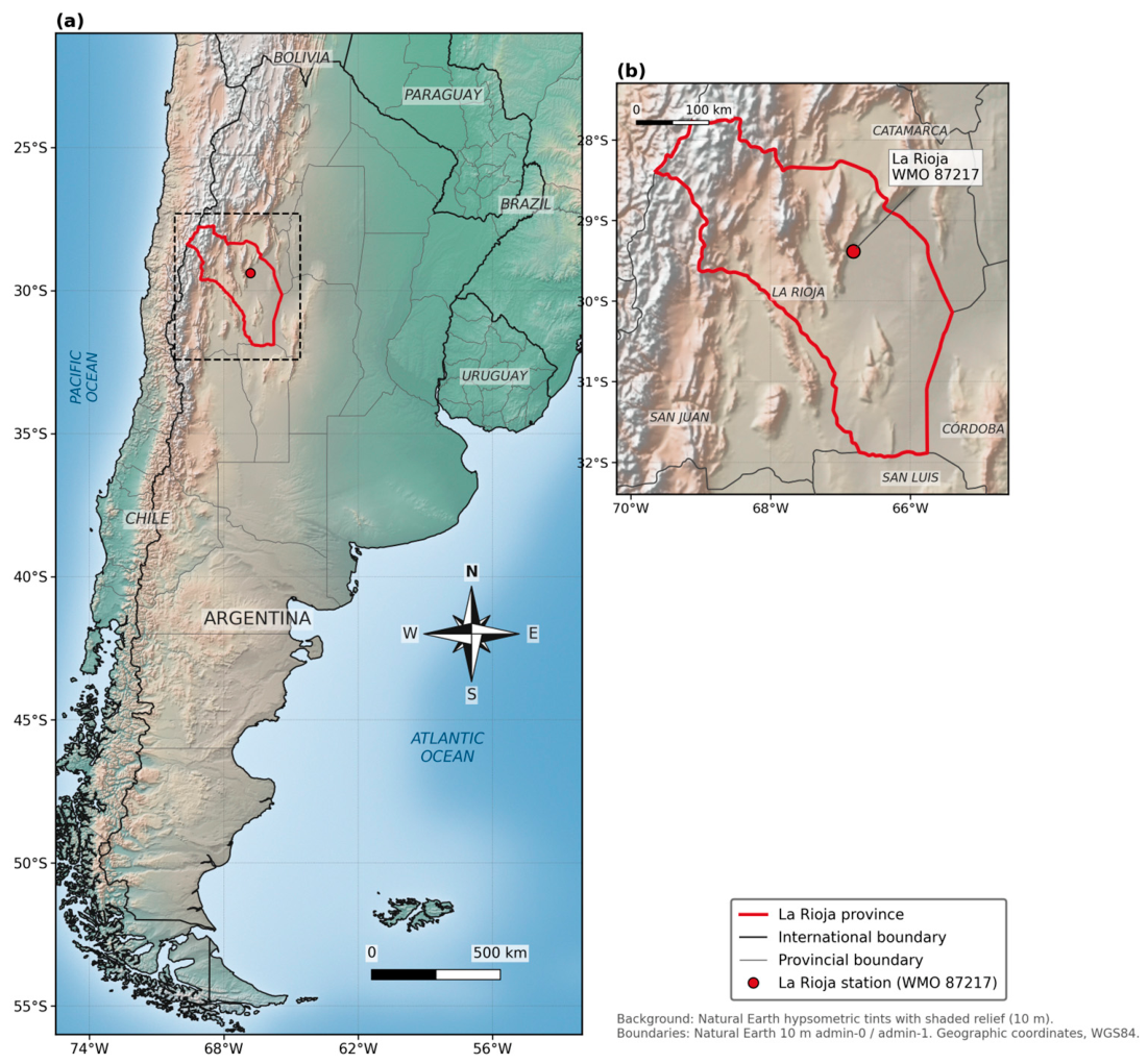
The study focuses on La Rioja (Figure 1), capital of the homonymous province in northwestern Argentina. The current observing station, La Rioja (WMO: 87217), is located at 29°23′ S, 66°49′ W, at an elevation of 429 m above sea level, on the eastern slope of the Sierra de Velasco within the Sierras Pampeanas geological system. The climate is classified as semiarid under the Köppen–Geiger scheme, characterised by hot summers with maximum temperatures frequently exceeding 40 °C, mild winters with occasional frost events, and mean annual precipitation of approximately 400 mm concentrated during the austral summer months (November–March). The marked continentality and aridity of the region result in large diurnal thermal amplitudes, making the site particularly suitable for studying the long-term behaviour and asymmetry of daily temperature extremes.

The daily maximum (Tmax) and minimum (Tmin) temperature series analysed here were constructed by merging two complementary data sources. The early portion of the record (1903–1940) was obtained from the historical archives of the Oficina Meteorológica Argentina (OMA), digitised and made publicly available through the Centre for Environmental Data Analysis (CEDA) as part of the Colonial Registers and Royal Navy Logbooks project [29]. The modern portion (1941–2019) corresponds to operational observations from the Servicio Meteorológico Nacional (SMN) for the La Rioja station. The two sources were combined into a continuous composite series for the 1903–2019 period, yielding a 117-year daily record.

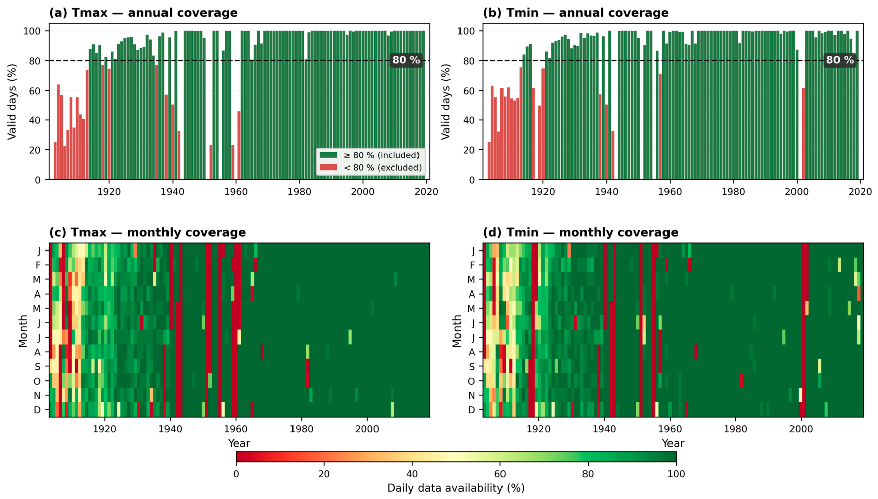
Non-climatic discontinuities in long temperature records may arise from changes in instrumentation, station relocation, modifications in observing practices, or changes in the surrounding environment [32]. To detect and correct such inhomogeneities, both series of temperature were subjected to a basic quality control and to homogeneity testing following the procedure described by Lakkis et al. [31] based on the joint application of four breakpoint detection tests to the daily series: the non-parametric Pettitt test, the Standard Normal Homogeneity Test (SNHT; [33]), the Buishand range test, and the Von Neumann ratio test [34]. As a result of the quality control, out of the 42,734 days in the study period, the composite series comprises 36,427 valid Tmax observations (85.2%) and 36,790 valid Tmin observations (86.1%). Missing values correspond to periods that were lost in the historical archive and to records that were removed during quality control, with their density substantially higher in the early decades than in the modern period (Figure 2). The homogeneity tests identified two breakpoints in the daily record: one in the Tmax series in October 2004 and one in the Tmin series in September 1944. Both series were then homogenised following the procedure adopted by Lakkis et al. [31], consistent with the WMO guidelines on homogenisation [32], by applying a constant additive adjustment to the subperiod preceding each breakpoint, taking the most recent subperiod as the homogeneous reference.

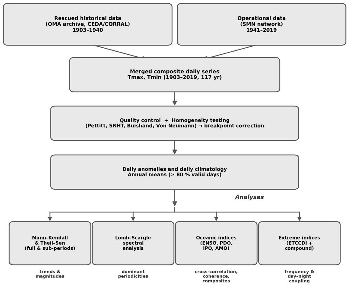
Figure 3 summarises the complete workflow followed in this study, from the construction and homogenisation of the composite series to the four complementary analyses described in the following sections.

2.2. Anomalies and Trend and Variability Analyses

Daily anomalies of Tmax, Tmin and DTR were obtained as the difference between each daily observation and the corresponding daily climatology, constructed by averaging the values recorded on the same calendar day of the year across the 117-year record. Daily climatological values calculated for the period of 1903–2019 were used to obtain deseasonalised temperature anomalies. Such an extended averaging period was selected, rather than the standard 30-year reference period, to take into account the considerable interannual to multidecadal variability observed in the temperature time series. Annual means were then obtained from the daily anomalies as follows: the average of the daily anomalies available within each year was added to the annual mean of the daily climatology, yielding the annual mean of the variable (Equation (1)).

$$\overline{T}\left(Y\right)=\overline{c} +{\displaystyle \frac{1}{n\_Y}}\sum _{d\in Y}\left[T \left(Y,d\right)-c\left(d\right)\right]$$

$$\overline{c}={\displaystyle \frac{1}{365}}{\displaystyle \sum _{d=1}^{365}}c\left(d\right)$$

(1)

$$c\left(d\right)= {\displaystyle \frac{1}{n\_d}}\sum _{\forall Y}T (Y,d)$$

Equations were considered both for Tmax and Tmin, in which $\overline{T} \left(Y\right)$ is the annual mean of the variable (Tmax or Tmin) for year Y, $\overline{c}$ is the annual mean constructed with the daily climatology (considering the total period), T(Y,d) is the temperature for year Y and calendar day d, and c(d) is the climatological value of Tmax or Tmin for calendar day d; n_Y is the number of days with valid temperature values in year Y, and n_d is the number of days with valid temperature values for calendar day d over the total period. As can be seen in Equation (1), the anomalies $\left[T\left(Y,d\right) - c\left(d\right)\right]$ were calculated for all the temperature values available for year Y and averaged for each year (Y). This deseasonalised treatment of the data yields an unbiased annual mean, even when the missing days are concentrated in particular months.

A year was considered valid only when at least 80% of its calendar days (≥292 days) had valid daily observations after the quality control and homogenisation procedures described above; years not meeting this threshold were excluded from the annual series.

The excluded years are concentrated in the early decades of the record, when the density of missing daily data was substantially higher; for both Tmax and Tmin, most fall within the period of 1903–1920, with a few additional isolated years in the mid-twentieth century and two recent years (2001–2002) additionally excluded for Tmin.

This procedure produces an unbiased annual mean, even when the missing days are concentrated in particular months of the year. Because the daily anomalies are already deseasonalised, gaps in any single month no longer bias the annual average toward warmer or colder seasons. Annual anomalies used in the subsequent trend and variability analyses were then defined as the deviation of each annual mean from the centennial mean computed over the valid annual series.

The presence and significance of trends in the annual series of Tmax, Tmin and DTR were evaluated using the non-parametric Mann–Kendall test (MK, [35,36]), which does not assume normality and is robust to outliers. The test was applied at the α = 0.05 significance level. The magnitude of each trend was quantified through the non-parametric Theil–Sen slope estimator (TS, [37,38]), defined as the median of the slopes between all pairs of points in the series; this estimator is insensitive to outliers and provides a robust estimate of the long-term rate of change. Both tests were applied to the annual series rather than to the daily series in order to avoid an increase in statistical significance produced by short-term serial autocorrelation.

To analyse the low-frequency variability of the annual series, two complementary smoothing procedures were applied. A centred 10-year moving-average filter was used to smooth the interannual variability while preserving the decadal and multidecadal signals. In parallel, robust locally weighted scatterplot smoothing (LOWESS; [39]) was applied to extract the same low-frequency behaviour under a different set of assumptions; the method fits local regressions at each point with a smoothing span of 0.20 of the series length, equivalent to an effective window of approximately 18 years for a 93-point series.

To characterise the dominant periodicities of the temperature variability, a Lomb–Scargle periodogram (LS, [40,41]) was computed on the deseasonalised daily anomaly series of Tmax, Tmin and DTR, taking advantage of the robustness of the LS method to irregular sampling. The LS method is a least-squares spectral analysis that fits sinusoidal components of different frequencies to the data and yields a power spectrum equivalent to the standard Fourier periodogram for evenly sampled series but defined and computable for unevenly sampled series. The analysis was performed on the deseasonalised daily anomalies so that the spectral peaks reflect interannual to multidecadal variability rather than the annual cycle; the statistical significance of each peak was evaluated through its false-alarm probability (FAP), and peaks were flagged as significant at the α = 0.05 level.

To investigate the influence of low-frequency oceanic variability on the temperature record, four climate indices were used: the El Niño-Southern Oscillation (ENSO; [15]), characterised through the Niño 3.4 index, captures the interannual variability of the tropical Pacific (typical periods of 3–7 years); the Pacific Decadal Oscillation (PDO; [17]), defined over the North Pacific, and the Interdecadal Pacific Oscillation (IPO; [22]), which extends over the entire Pacific basin, represent the lower-frequency expression of Pacific variability, both operating on decadal to multidecadal timescales (~20–40 years); and the Atlantic Multidecadal Oscillation (AMO; [24]) captures multidecadal sea-surface temperature variability of the North Atlantic, with periods typically around 50–80 years. The four indices are physically related, in part, but operate at distinct dominant timescales, providing complementary diagnostics of oceanic forcing at the periodicities relevant to the multidecadal variability identified in the temperature record. Annual values of the four indices, spanning the full 1903–2019 study period, were obtained as the arithmetic mean of the 12 monthly values of each calendar year, computed from the original monthly series downloaded from NOAA’s Physical Science Laboratory (https://psl.noaa.gov/ accessed on 20 February 2026).

To assess the relationship between those indices and the temperature variability at La Rioja, two complementary tools were applied to the annual series. First, lagged Pearson cross-correlations were computed between each anomaly series and each index for lags ranging from −15 to +15 years. Statistical significance of the cross-correlation at a lag of zero was assessed using a t-test based on the effective sample size [42] to account for serial autocorrelation. Because four indices were tested simultaneously, a Bonferroni correction [43,44] was applied, reducing the significance threshold from the nominal 0.05 to 0.0125 (α/k) to account for multiple testing. Second, magnitude-squared spectral coherence was computed by Welch’s method [45] using Hann windows of 40 years with 50% overlap; this analysis quantifies the frequency-by-frequency covariance between each pair of series and provides evidence of shared variability at specific timescales, independent of the time-domain correlation. Coherence values greater than 0.5 were interpreted as indicative of strong spectral covariance, while the cross-correlation and Bonferroni-adjusted significance were retained as the primary diagnostic; the coherence spectrum was used as secondary, frequency-resolved evidence.

Additionally, a composite analysis was performed to provide a non-parametric corroboration of the linear correlation results. Each year was classified as a positive, negative or neutral phase of each oceanic index using a threshold of ±0.5 standardised units (z-scores computed over the full 1903–2019 record of each index), and the mean annual anomaly of each temperature variable (Tmax, Tmin and DTR) was computed within each phase. The statistical significance of the difference between positive and negative composites was assessed by a bootstrap permutation test with 10,000 iterations.

2.3. Extreme Temperature Events

A set of indices was used to characterise the temporal evolution of extreme temperature events over the study period, following the standard definitions established by the Expert Team on Climate Change Detection and Indices (ETCCDI; [46]). First, four frequency indices were considered: TX90p and TX10p, defined as the annual percentage of days on which Tmax exceeded the 90th percentile (warm days) or fell below the 10th percentile (cold days) of its calendar-day distribution, and TN90p and TN10p, defined analogously for Tmin (warm and cold nights). The calendar-day thresholds were obtained from a five-day moving window centred on each day of the year across the full 1903–2019 record in order to vary smoothly with the seasonal cycle and rest on a sufficiently large sample. Together, these four indices describe the relative frequency of the four extreme regimes and allow the day–night asymmetry of changes in extremes to be assessed, as warm days, cold days, warm nights and cold nights can evolve independently and reflect distinct physical mechanisms.

Compound day–night indices were also computed to characterise the joint behaviour of the diurnal cycle under extreme conditions. The compound warm-day index was defined as the annual percentage of days on which Tmax and Tmin simultaneously exceeded their respective 90th percentiles, while the compound cold-day index is its analogue below the 10th percentiles (Equation (2)).

$$\begin{gathered} CWD=(100/N) {\displaystyle {\sum }_{d=1}^N}I\left[T_{max}\right(d)>P_{90max}(d) \wedge T_{min}(d)>P_{90min}(d\left)\right] \\ CCD=(100/N) {\displaystyle \sum _{d=1}^N}I\left[T_{max}\right(d)<P_{10max}(d) \wedge T_{min}(d)<P_{10min}(d\left)\right] \end{gathered}$$

(2)

where N is the number of valid days in the year, I [] is the indicator function (equal to 1 when the condition in brackets is satisfied and 0 otherwise), P90_max(d) and P90_min(d) are the calendar-day 90th percentiles of Tmax and Tmin respectively, and P10_max(d) and P10_min(d) are the corresponding 10th percentiles. The ∧ symbol denotes the logical “and” so that a day is counted only when both the daytime and nighttime extreme conditions are met simultaneously.

This dual-threshold criterion captures days on which extreme daytime conditions are not relieved by an opposite extreme nighttime regime, a configuration recognised as having severe consequences for human health and ecosystem stress [47,48]. The strength of the day–night coupling under extreme conditions was further quantified by the co-occurrence ratio, defined as the ratio between the observed compound frequency and the frequency that would be expected if the daytime and nighttime extremes were statistically independent (Equation (3)).

$$R=f_{obs} / f_{exp}=f_{obs} / (f_{day}\times f_{night})$$

(3)

where $f_{obs}$ is the observed annual frequency of compound extreme days and $f_{exp}$ =$f_{day} \times f_{night}$ is the frequency expected under statistical independence, with $f_{day}$ and $f_{night}$ representing the marginal frequencies of the daytime and nighttime extremes respectively. All three frequencies are expressed as annual fractions (proportions of valid days, 0–1) so that the product of $f_{day}$ × $f_{night}$ is dimensionally consistent. A ratio of R > 1 indicates that daytime and nighttime extremes co-occur more often than expected by chance.

The temporal evolution of each index was analysed using the MK test and the TS slope estimator as previously described, with trends expressed in units of % of days per century.

2.4. Use of Generative AI Tools

During the preparation of this manuscript, the authors used Claude, developed by Anthropic (Opus 4.8), to generate Figure 1, which shows a map of the study area and its description, and Figure 2, which shows the annual and monthly coverage of data corresponding to the daily Tmax and Tmin records in La Rioja. The authors have reviewed and edited the output and accept full responsibility for the content of this publication.

3. Results

3.1. Annual Mean Temperatures and Long-Term Trends

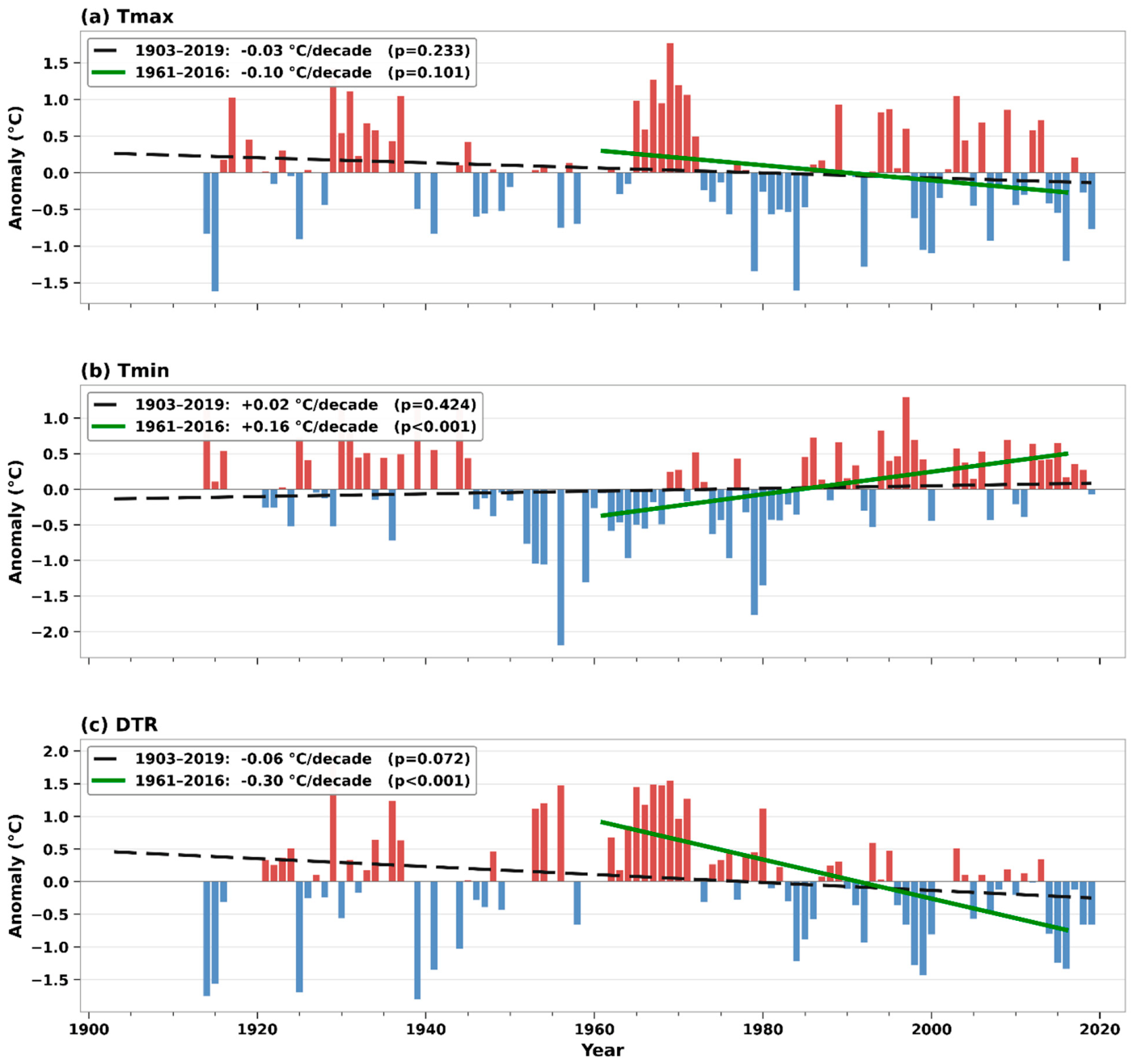
The annual series of Tmax, Tmin and DTR for the 1903–2019 period are shown in Figure 4, with TS trend lines fitted to the full period and to the 1961–2016 subperiod. The series show marked interannual variability superimposed on a low-frequency oscillatory pattern.

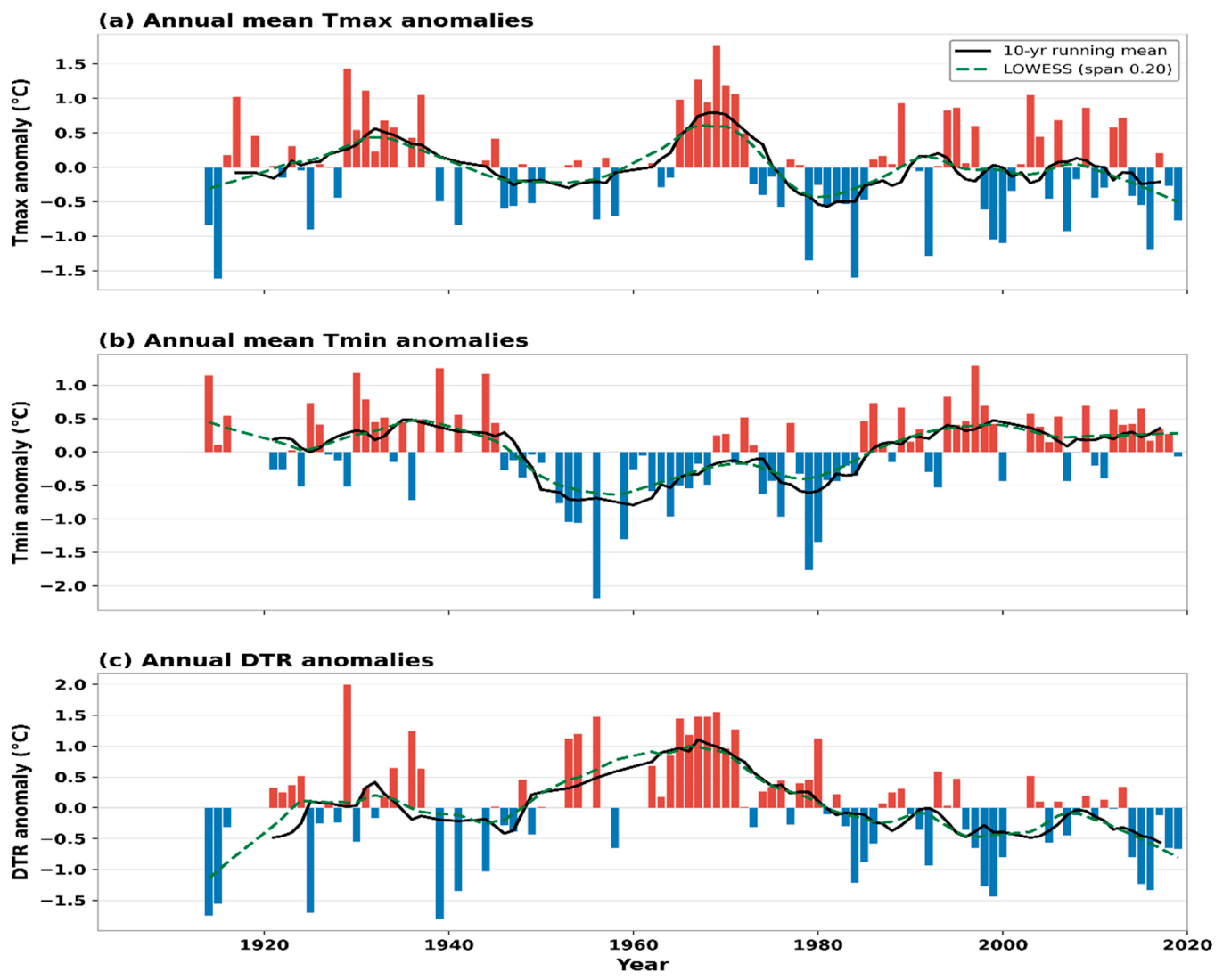
Figure 4 displays the same annual series as anomalies relative to the centennial mean, smoothed with a centred 10-year moving average (black line) and a LOWESS curve (green dashed line). This stationarity at the centennial scale coexists with a marked low-frequency pattern. The Tmax series shows extended warm intervals around the late 1920s and the late 1960s, with the latter standing out as the most prominent positive episode of the record, separated by cooler decades in the 1950s and a return to lower values in the 1980s. The Tmin series shows a pronounced extended cold phase between approximately 1945 and 1985, flanked by warmer conditions before and after; the post-1990 segment exhibits the highest sustained mean values of the record. The DTR closely tracks the Tmax behaviour in its first half but inverts after the mid-1970s, with a sustained decrease that persists until the end of the record.

The MK test (

Table 1. Trend statistics for the annual series of Tmax, Tmin and DTR at La Rioja. For each variable (first column) and each analysis period (second column: the full study period of 1903–2019 and the recent 1961–2016 and 1961–2019 subperiods), the table reports: n, the number of valid annual values in the window; Kendall’s τ, the non-parametric rank-correlation statistic of the MK test, whose sign indicates the direction of the trend; the associated p-value of the MK test; and the TS slope, expressed in °C per decade, which quantifies the magnitude of the trend. Statistically significant trends at α = 0.05 are highlighted in bold.

Variable	Period	n	Kendall’s τ	p-Value	TS Slope (°C/Decade)
Tmax	1903–2019	93	−0.084	0.233	−0.03
	1961–2016	55	−0.153	0.101	−0.10
	1961–2019	58	−0.160	0.077	−0.10
Tmin	1903–2019	93	+0.057	0.424	+0.02
	1961–2016	54	+0.338	<0.001	+0.16
	1961–2019	57	+0.316	<0.001	+0.14
DTR	1903–2019	88	−0.131	0.072	−0.06
	1961–2016	53	−0.401	<0.001	−0.30
	1961–2019	56	−0.413	<0.001	−0.29

) indicates that none of the three variables displays a statistically significant trend over the centennial period. Thus, at the centennial scale, the daytime, nighttime and diurnal-range temperature means at La Rioja are stationary. Long-term trends can be strongly influenced by the temporal window over which they are computed. Linear trend analysis implicitly assumes a constant rate of change throughout the analysis window, and this assumption is recognised as restrictive for climate variables whose evolution is characterised by strong non-stationarity and pronounced low-frequency variability [49]. In such cases, a trend computed over one window can differ substantially from a trend computed over another simply because each window samples a different portion of the underlying multidecadal cycle; a subperiod that begins near a cold phase and ends near a warm phase will yield an apparent warming trend, while another that captures a full multidecadal oscillation will yield an apparently stationary trend. Canziani et al. [50], analysing centennial precipitation records from four Argentine stations, reached a similar conclusion: linear trends and 30-year reference periods, while useful as summary descriptors, reach their methodological limits in climate variables dominated by multidecadal variability and non-linear evolution. To assess the sensitivity of the trend results to the analysis window, the MK test and the TS slope estimator were also applied to two recent subperiods: 1961–2016, which corresponds to the temporal window most commonly adopted in regional studies of Argentine and South American temperature trends, and 1961–2019, which extends the analysis to the end of the available record. The results are also reported in Table 1 and Figure 4 and show that the picture changes substantially when the analysis is restricted to the recent decades. Over the period of 1961–2016, Tmin exhibits a strongly significant warming trend, with a TS slope of +0.16 °C per decade, while the DTR exhibits a strongly significant decrease, with a TS slope of −0.30 °C per decade. Extending the window to 1961–2019 yields virtually identical results (Tmin +0.14 °C per decade and DTR −0.29 °C per decade, both significant at p < 0.001), confirming that the recent trends are robust to the choice of end year. In contrast, Tmax remains essentially stationary in all three windows.

These results—in particular, those for the 1961–2016 window used in previous regional studies—are quantitatively consistent with previous reports for the Argentine and South American domains, where the bulk of the regional warming signal originates in the nighttime regime [7,8,10].

To further characterise the interannual variability of the record, the five warmest and coldest years in terms of annual Tmin anomalies were identified (

Table 2. Top 5 warmest and coldest years in La Rioja based on annual minimum and maximum temperature anomalies (°C) relative to the historical baseline.

Position	Warmest Years	Coldest Years
1	1997 (+1.29)	1956 (−2.19)
2	1939 (+1.26)	1979 (−1.76)
3	1930 (+1.18)	1980 (−1.35)
4	1944 (+1.17)	1959 (−1.31)
5	1914 (+1.15)	1954 (−1.06)

). Focusing on Tmin isolates the nighttime regime, which dominates the regional warming signal and avoids the masking effect of daytime variation. The warmest nighttime year on record is 1997 (+1.29 °C above the centennial mean), coinciding with the onset of one of the most intense El Niño events of the twentieth century, plausibly associated with increased nocturnal cloud cover and reduced longwave radiative cooling. Two other prominent warm years were 1939 (+1.26 °C) and 1930 (+1.18 °C). Conversely, the most severe negative anomalies are concentrated in the mid-twentieth century. The coldest year was 1956, with an anomaly of −2.19 °C, followed by 1979 (−1.76 °C) and 1980 (−1.35 °C). Notably, three of the five coldest years on record occurred within the 1950s (1954, 1956 and 1959), pointing to a sustained cold cluster whose characterisation is taken up by the spectral analysis presented in the following section.

3.2. Multidecadal Variability and Dominant Periodicities

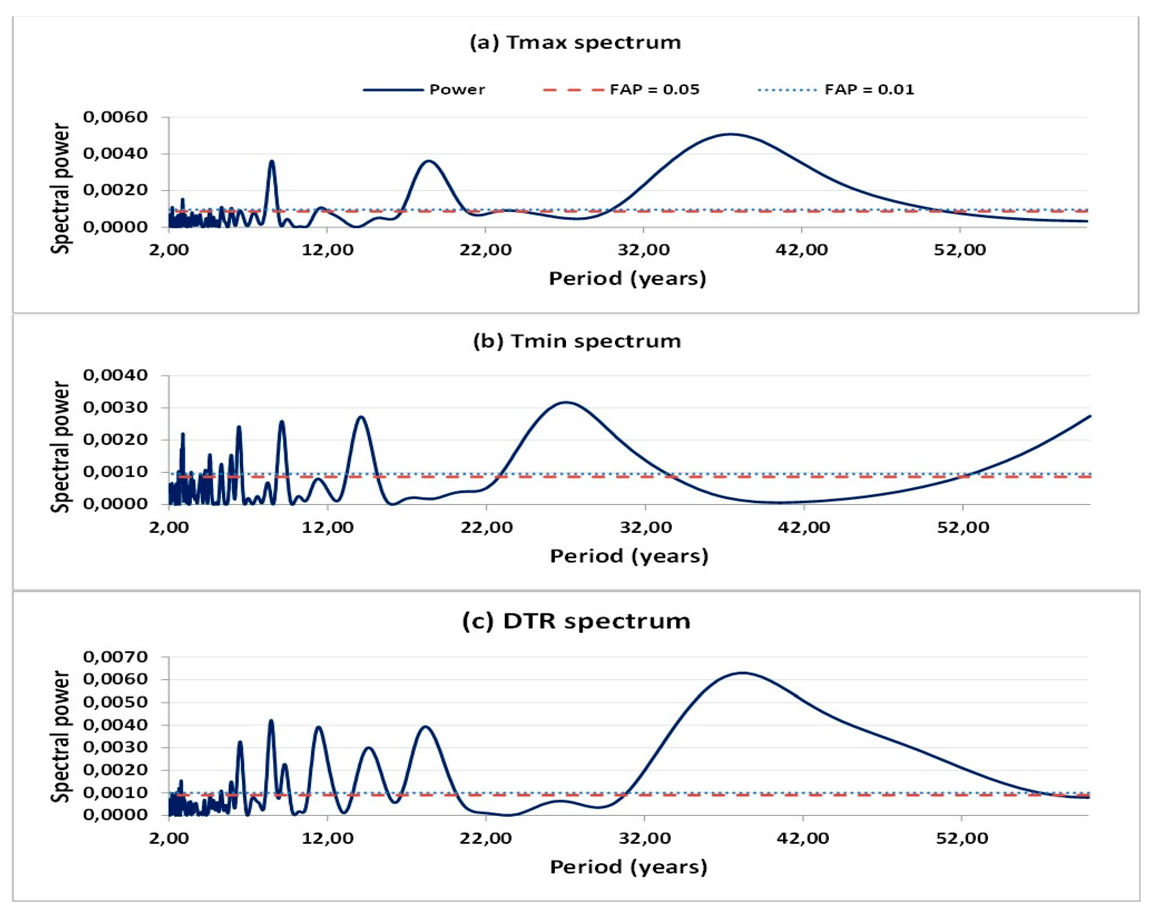
The low-frequency oscillatory pattern shown in Figure 5 was further characterised by computing the LS power spectrum of the deseasonalised daily anomaly series of Tmax, Tmin and DTR (Figure 6). The three spectra share a common qualitative feature with a dominant peak in the multidecadal band, well above the threshold at α = 0.01, alongside secondary patterns at decadal and interannual scales. For Tmax (Figure 6a), the dominant peak is located at a period of approximately 37–38 years. Secondary significant peaks are found in the decadal band, most prominently around 18 years, with additional structure present in the interannual band including a peak near the typical ENSO periodicity of 5–7 years. The Tmin spectrum (Figure 6b) is dominated by a peak at approximately 27 years, also far above the 1% significance threshold, with additional significant peaks distributed across the decadal band (around 18, 13–14 and 11 years) and a more diffuse interannual signal. The DTR spectrum (Figure 6c) exhibits the strongest multidecadal peak of the three series, again at approximately 37–38 years and with a peak power higher than that of either Tmax or Tmin, alongside secondary peaks near 18 and 14 years and additional interannual structure.

3.3. Association with Oceanic Indices

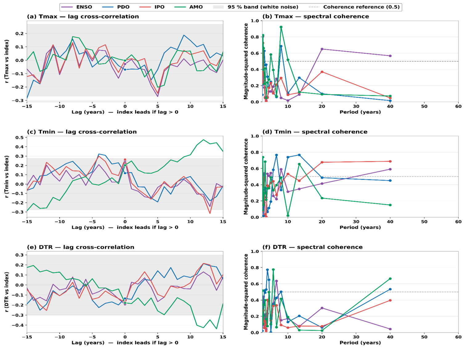
The multidecadal variability identified in the previous section motivates the question of whether this low-frequency variability is coupled with known modes of oceanic origin. The dominant spectral peaks found around 27 years for Tmin and 37 years for both Tmax and DTR occur at timescales comparable to those of the major modes of Pacific and Atlantic decadal to multidecadal variability. The relationship between the temperature record and those indices was examined through two complementary analyses: lagged cross-correlation in the time domain and spectral coherence in the frequency domain (Figure 7). The results show a remarkable contrast between the three temperature variables. The Tmax series (Figure 7a,b) shows no statistically significant association with any of the four indices. Lag-zero correlations are weak in absolute value and lie within the 95% white-noise confidence band for all four modes (|r| ≤ 0.07; p > 0.5 in each case). The coherence spectrum exhibits scattered peaks but no consistent pattern across timescales. Therefore, at the annual scale analysed here, the daytime temperature behaviour at La Rioja shows no consistent linear association with any of the four considered large-scale oceanic modes. The Tmin series (Figure 7c,d), on the other hand, presents a substantially different picture. The two indices associated with the tropical Pacific (ENSO and IPO) display positive lag-zero correlations of comparable magnitude (r = +0.249, p = 0.028 for ENSO; r = +0.264, p = 0.020 for IPO), with significance assessed using the effective sample size after correction for serial autocorrelation. Both values lie at or slightly beyond the upper edge of the 95% white-noise band. PDO (r = +0.117, p = 0.354) and AMO (r = +0.202, p = 0.146) do not reach significance at the 5% level. After applying a Bonferroni correction for the four simultaneous tests (effective threshold α/k = 0.0125), neither ENSO nor IPO formally meets the multiple-comparison-adjusted criterion, although the consistency between two independent but related indices of Pacific variability strengthens the empirical case for a real, if modest, coupling. The coherence spectrum reinforces this picture; over multidecadal periods (around 20–40 years), PDO, IPO and ENSO all attain coherence values close to or above 0.5, indicating substantial shared variability between Tmin and tropical Pacific variability at the timescales previously identified as dominant in the Tmin record. AMO coherence is weaker during those periods.

The DTR series (Figure 7e,f) shows lag-zero correlations that are uniformly negative across the four indices (between −0.13 and −0.19), but none reaches statistical significance at the 5% level (smallest p = 0.10, ENSO). The sign of these correlations is consistent with the Tmin result; warm phases of the Pacific tend to be associated with warmer nights, compressing the diurnal range. The coherence spectrum of the DTR with the four indices is weaker than that of the Tmin, with most values below 0.5 across the range of resolved periods.

To complement the previous analyses with a non-parametric perspective, a composite analysis was performed by classifying each year of the record into positive, negative or neutral phases of each oceanic index (threshold ±0.5 standardised units) and computing the mean anomaly within each phase for the three temperature variables (

Table 3. Composite analysis of annual anomalies of Tmax, Tmin and DTR at La Rioja (1903–2019), conditional on the phase of each oceanic index. Each year was classified as a positive (Pos), negative (Neg) or neutral phase using a threshold of ±0.5 standardised units (z-scores computed over the full 117-year record of each index). Columns give the number of years per phase, the mean anomaly within each phase, the difference between positive and negative composites (Δ), and the p-value from a bootstrap permutation test of the difference. Statistically significant differences at α = 0.05 are highlighted in bold.

Variable	Index	n (Pos)	Mean Pos (°C)	n (Neg)	Mean Neg (°C)	Δ (°C)	p
Tmax	ENSO	34	+0.02	28	−0.03	+0.04	0.820
	PDO	25	−0.05	29	+0.02	−0.07	0.704
	IPO	27	+0.06	29	+0.02	+0.05	0.799
	AMO	34	−0.08	27	−0.08	0.00	0.993
Tmin	ENSO	32	+0.19	28	−0.22	+0.41	0.014
	PDO	26	+0.09	28	−0.12	+0.20	0.262
	IPO	24	+0.25	27	−0.19	+0.44	0.012
	AMO	36	+0.22	25	−0.11	+0.33	0.055
DTR	ENSO	32	−0.14	27	+0.22	−0.35	0.104
	PDO	24	−0.16	27	+0.12	−0.28	0.235
	IPO	24	−0.14	27	+0.21	−0.35	0.130
	AMO	33	−0.31	25	+0.02	−0.33	0.132

). For Tmax, all four composite differences are virtually zero and non-significant (p > 0.7), confirming the decoupling already suggested by the linear correlation. For Tmin, ENSO (Δ = +0.41 °C, p = 0.014) and IPO (Δ = +0.44 °C, p = 0.012) yield significant differences, while AMO shows a comparable magnitude but only marginal significance (Δ = +0.33 °C, p = 0.055) and PDO remains non-significant. For DTR, all four composite differences are negative and not significant, consistent with the absence of modulation in Tmax, combined with the Tmin response.

3.4. Extreme Temperature Events Analysis

The frequency of extreme temperature events at La Rioja was characterised through the four ETCCDI percentile-based indices, two compound day–night indices computed as described in the Methodology (Figure 8,

Table 4. MK test and TS slope estimates for the six extreme temperature indices computed for the La Rioja record (1903–2019). Statistically significant trends at α = 0.05 are highlighted in bold. The TX90p index displays the strongest signal.

Index	Mean	Kendall’s τ	p	TS Slope (per Century)
TX90p (warm days)	9.98%	−0.199	0.005	−3.82%
TN90p (warm nights)	9.62%	+0.113	0.110	+2.00%
TX10p (cold days)	9.66%	−0.024	0.732	−0.32%
TN10p (cold nights)	9.97%	+0.047	0.509	+0.75%
Compound warm days	3.70%	−0.139	0.055	−1.30%
Compound cold days	2.13%	−0.053	0.466	−0.21%

). Together, the six indices describe the evolution of extremes through their frequency and day–night coupling.

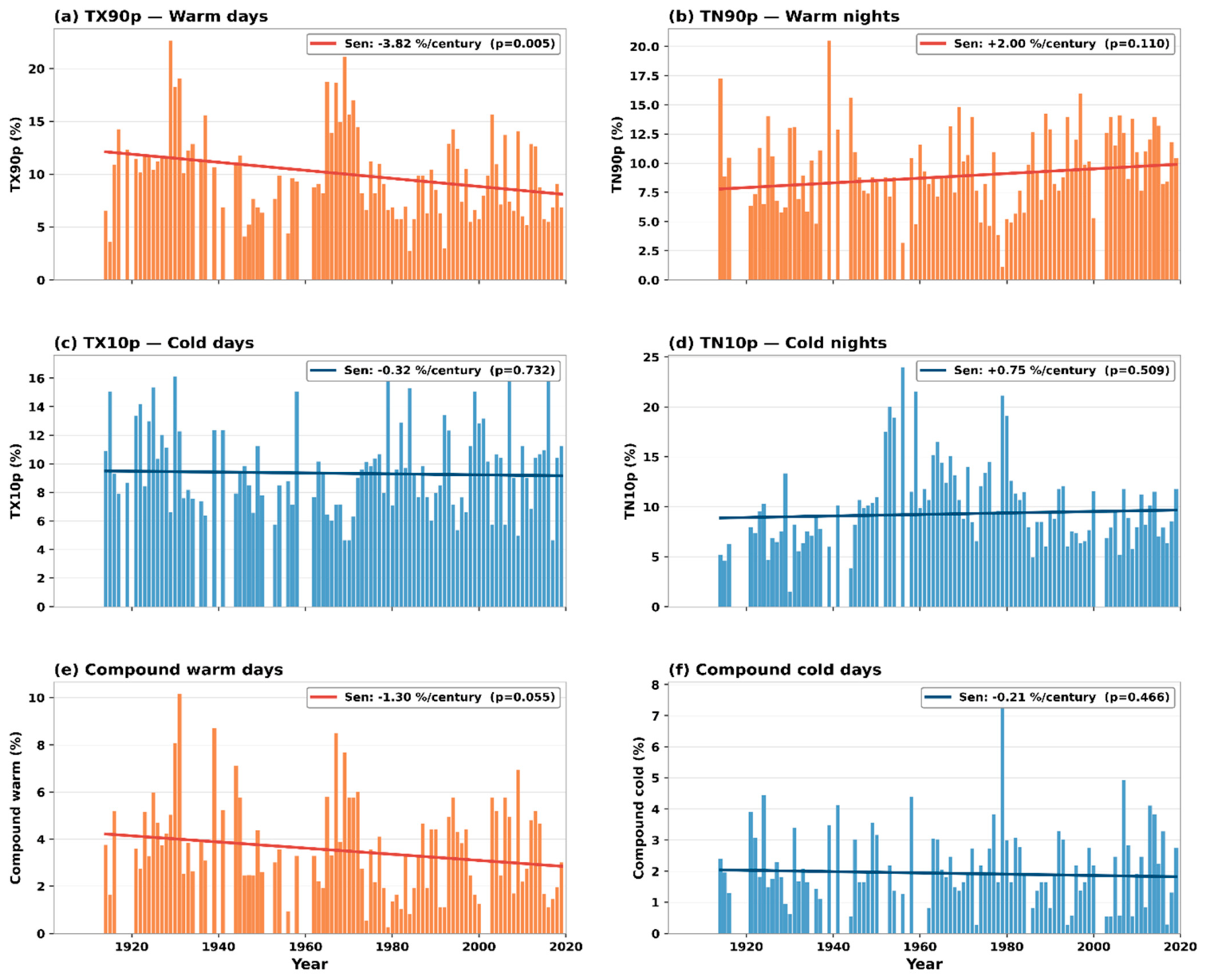
The strongest signal among the percentile-based indices is a statistically significant decrease in the frequency of warm days (TX90p; TS slope: −3.82% per century; p = 0.005; Figure 8a), consistent with the absence of a centennial warming trend in the underlying Tmax series. The frequency of warm nights (TN90p, Figure 8b) shows a positive TS slope of +2.00% per century, but this trend is not statistically significant at the 5% level. The frequencies of cold days (TX10p) and cold nights (TN10p, Figure 8c,d) show no statistically significant trend (p > 0.5 in both cases). Cold extremes at La Rioja—both daytime and nighttime—remained stationary over the 1903–2019 period.

The two compound day–night indices show negative TS slopes, with that for the compound warm days approaching but not reaching the 5% significance level (−1.30% per century, p = 0.055, Figure 8e), while the compound cold days show no trend (p = 0.466, Figure 8f). The change in the extreme behaviour is therefore concentrated in the frequency of moderate daytime warm days rather than in the joint day–night extremes.

A complementary diagnostic is provided by the co-occurrence ratio, which compares the observed frequency of compound day–night extremes with that expected under statistical independence of the daytime and nighttime extreme regimes. The observed mean annual frequency of compound warm days (3.70%) is 3.85 times higher than the value expected under independence (0.96%), and the corresponding ratio for compound cold days is 2.21. Both ratios are well above unity, indicating that daytime and nighttime extremes at La Rioja occur together several times more often than would be expected by chance. This coupling is nonetheless far from systematic; of all the extreme warm days in the record, only 37.7% were followed by an extreme warm night, and for cold days, the corresponding fraction is even lower (22.6%), so the majority of extreme daytime events are not mirrored at night. Therefore, the day–night coupling describes a strong statistical tendency rather than a rule, and it is markedly stronger for warm extremes than for cold ones. This asymmetry is not obvious a priori and could be linked to the different physical controls on daytime and nighttime temperatures: warm extremes could be associated with persistent anticyclonic conditions and dry air that affect both day and night, whereas cold daytime extremes could be followed by radiative nighttime recovery that prevents an extreme cold night. However, a detailed attribution of these mechanisms lies beyond the scope of the present observational study.

Beyond their long-term trends, the extreme indices display substantial interannual variability. The warm-day frequency (TX90p) ranges from 2.7% (1984) to 22.6% (1929), and the warm-night frequency (TN90p) ranges from 1.1% (1979) to 20.5% (1939), while the cold-night frequency (TN10p) spans the widest range, from 1.5% (1930) to 24.0% (1956). Certain periods stand out owing to their concentration of extremes: the 1920s and 1930s recorded the highest warm-day frequencies, whereas the 1950s were marked by an exceptional frequency of cold nights, peaking in 1956. This cold-night maximum coincides with the sustained cold cluster identified in the annual Tmin series in Section 3.1 and with the negative phase of the Pacific oscillations preceding the 1976/77 climate shift, while the warm-night maximum of 1939 corresponds to one of the warmest years in the Tmin record (Table 2). The year 1979 also stands out as a distinctly cold one in the nighttime regime, combining the lowest warm-night frequency with the highest compound cold-day frequency of the record. These fluctuations appear consistent with the multidecadal modulation of nighttime temperature discussed in Section 3.3, suggesting that the year-to-year and decadal variability of the extreme indices may be linked to the same low-frequency processes associated with the mean series.

4. Discussion

In this study, 117 years of rescued observations of daily maximum and minimum temperature from La Rioja (1903–2019) were analysed to characterise the long-term temperature evolution at this semiarid site of northwestern Argentina, with particular emphasis on disentangling trends, multidecadal variability and changes in the extreme regime. Over the full 1903–2019 period, none of the three series of Tmax, Tmin or DTR displays a statistically significant trend, and the centennial mean of the three series at this station can therefore be characterised as stationary. However, trends depend strongly on the analysis window. When the MK and TS analyses are restricted to the recent decades, the warming of Tmin and the narrowing of the DTR reappear in a manner quantitatively consistent with previous regional reports, since the time periods of 1961–2016 and 1961–2019 yield virtually identical results.

Results show a marked asymmetry between the daytime and nighttime temperature behaviour. Although both the daytime and nighttime means are stationary over the centennial period, the subperiod analysis reveals that the source of the recent regional warming lies almost entirely in the nighttime regime, while Tmax remains stable. In the spectral domain, both series exhibit dominant multidecadal peaks but at different periodicities, suggesting that distinct low-frequency processes modulate the two variables. The same contrast appears in the extremes, where the frequency of warm days declines significantly while the frequency of warm nights shows a non-significant positive tendency. This day–night asymmetry is consistent with the well-known fact that daytime and nighttime temperatures respond to different combinations of physical processes; daytime maxima are dominated by incoming solar radiation and turbulent mixing within the convective boundary layer, while nighttime minima are more sensitive to the radiative balance of the nocturnal boundary layer, which, itself, depends on humidity, cloud cover and circulation. Although several of these processes affect both regimes, their relative contributions differ between day and night, and disentangling them in the observed temporal asymmetry would require dedicated multivariate analysis beyond the scope of the present study. A similar day–night asymmetry across diagnostic indices has been reported across the South American domain [7,10].

The association between this multidecadal variability and the oceanic modes deserves closer examination. The multidecadal variability of the record is partly but not entirely linked to the four considered oceanic modes. ENSO and IPO yield comparable positive correlations with Tmin, both of which are significant. The coherence spectrum further shows that the shared variability is concentrated in multidecadal periods, i.e., at the timescales of the dominant spectral peaks of the Tmin series. This suggests that the multidecadal Tmin variability at La Rioja contains a footprint of tropical Pacific decadal forcing, although the physical origin cannot be settled from these data alone. In contrast, no comparable annual-scale association was found between Tmax and the four oceanic indices, suggesting that, at the analysed temporal resolution, the daytime regime does not respond consistently to these modes. The composite analysis (Table 3) corroborates this interpretation with a non-parametric tool; the four composite differences in Tmax are negligible (all p > 0.7), confirming the absence of an annual-scale association between the daytime regime and the four oceanic modes, while for Tmin, the differences with ENSO (+0.41 °C) and IPO (+0.44 °C) are both statistically significant. The composite signal for AMO on Tmin is of comparable magnitude (+0.33 °C) but only marginally significant (p = 0.055), suggesting a possible influence not detected by the linear correlation analysis. Three of the five warmest nighttime years in the record are associated with positive ENSO phases (1997, 1930, 1914), and three of the five coldest cluster in the 1950s (1954, 1956 and 1959), preceding the well documented 1976/77 Pacific climate shift [19,21].

The analysis of extreme temperature events reinforces the picture obtained from the means while adding a feature that the centennial averages do not reveal. The frequency of warm days (TX90p) declines significantly over the study period, even though the Tmax centennial mean is stationary, suggesting that hot extremes have become less frequent, while the daytime temperature on a typical day has not changed.

The frequencies of cold days and cold nights show no trend; the change is therefore concentrated in the frequency of moderate daytime warm days. The compound day–night indices reveal a different aspect; the co-occurrence ratios for both warm and cold compound days are well above unity, indicating that joint day–night extremes at La Rioja occur several times more often than under statistical independence, although the coupling represents a statistical tendency rather than a rule, since most extreme daytime events are not mirrored at night. Moreover, this tendency is stronger for warm extremes than for cold ones, an asymmetry that points to distinct physical controls on the daytime and nighttime regimes.

The behaviour observed at La Rioja can be placed in the context of the broader literature on diurnal temperature asymmetry. Braganza et al. [51], combining global gridded observations from the Climatic Research Unit with coupled climate model simulations, established that the DTR is a robust proxy of climate change over the twentieth century and showed that its observed reduction is unlikely to be explained by natural variability alone. Several authors, such as Karl et al., Vose et al., and Davy et al. [2,4,52], among others, have also noted a widespread decline of the DTR over most global land areas since the 1950s, driven by the faster warming of Tmin than Tmax. The physical mechanisms proposed in these studies are based on changes in cloud cover, soil moisture, precipitation and boundary-layer processes and are coincident with those invoked here. At the regional scale, our results agree well with those reported by Vincent et al. [7], whose analysis of daily station observations across South America found that the continental warming signal was carried mainly by the nighttime regime, with a significant increase in warm nights but weaker or non-significant changes in daytime extremes. Using the China Meteorological Administration land-surface temperature dataset for 1901–2018, Sun et al. [53] found that the DTR for East Asia decreased by about 0.60 °C over the full period of study but that this decline was concentrated in the second half of the twentieth century in the earlier decades with marked interdecadal fluctuations. Note that the period of time is similar to the one we report here for La Rioja, with the significant DTR reduction confined to the recent decades while the centennial record is dominated by multidecadal variability. The study also linked the low-frequency variability of nighttime temperature to multidecadal oceanic influence, including the AMO, in agreement with the associations discussed here.

More recently, using observation datasets, Zhong et al. [5] reported a reversal of this asymmetry over the last three decades, with accelerated warming of Tmax and an increase in the DTR across more than half of the Earth’s land surface, most pronounced in Europe, Australia and North America, which they attributed largely to a reduction in cloud cover.

5. Conclusions

This study illustrates that trend analysis alone is not sufficient to fully characterise long-term climate variability, since linear trends may overlook multidecadal oscillations, cyclic behaviour and changes in extremes. By complementing the MK test and TS trend assessment with spectral analysis, oceanic index diagnostics and extreme event indices, the present analysis aims to distinguish long-term signals from natural low-frequency fluctuations in the 117-year temperature record of La Rioja. The main findings can be summarised as follows:

• Over the full 1903–2019 period, the annual means of Tmax, Tmin and DTR are stationary, yet the record is dominated by pronounced multidecadal variability, with spectral peaks near 37 years for Tmax and DTR and 27 years for Tmin.
• The nighttime regime is weakly but consistently associated with tropical Pacific variability (ENSO and IPO), whereas the daytime regime shows no such association.
• A significant decline in the frequency of warm days coexists with the stationary Tmax mean, revealing a day–night asymmetry that runs through all diagnostics.

This combination of centennial stationarity and a DTR decrease is confined to the recent decades: the multidecadal variability that dominates the full record may reflect the same low-frequency processes, including the oceanic modes examined here, that modulate the strength and even the sign of the diurnal asymmetry over multidecadal timescales. In this respect, the La Rioja record, as a long and continuous series of daily station observations from a semiarid region of the Southern Hemisphere, where such records are scarce and where the recent global datasets show the least agreement, contributes a valuable observational reference to a debate that has, so far, relied predominantly on northern hemisphere and gridded data.

Finally, some limitations should be acknowledged. The analysis addresses stationarity in the mean, while potential changes in higher-order moments, such as the variance or asymmetry of the distributions, were not assessed, and the association with oceanic modes was examined at annual scale, so seasonally resolved relationships or modulations by other circulation patterns may exist that the annual aggregation does not capture.

Beyond its methodological contribution, by providing a long-term observational reference for a semiarid, data-sparse region, this study may also help to inform climate risk assessment and adaptation planning in northwestern Argentina, where the characterisation of multidecadal variability and of changes in temperature extremes is particularly relevant for the agricultural and water-resource sectors.

References

1. IPCC. Climate Change 2021: The Physical Science Basis. Contribution of Working Group I to the Sixth Assessment Report of the Intergovernmental Panel on Climate Change; Masson-Delmotte, V., Zhai, P., Pirani, A., Connors, S.L., Péan, C., Chen, Y., Goldfarb, L., Gomis, M.I., Matthews, J.B.R., Berger, S., et al., Eds.; Cambridge University Press: Cambridge, UK, 2021. [Google Scholar]
2. Karl, T.R.; Jones, P.D.; Knight, R.W.; Kukla, G.; Plummer, N.; Razuvayev, V.; Gallo, K.P.; Lindseay, J.; Charlson, R.J.; Peterson, T.C. A new perspective on recent global warming: Asymmetric trends of daily maximum and minimum temperature. Bull. Am. Meteorol. Soc. 1993, 74, 1007–1023. [Google Scholar] [CrossRef]
3. Easterling, D.R.; Horton, B.; Jones, P.D.; Peterson, T.C.; Karl, T.R.; Parker, D.E.; Salinger, M.J.; Razuvayev, V.; Plummer, N.; Jamason, P.; et al. Maximum and minimum temperature trends for the globe. Science 1997, 277, 364–367. [Google Scholar] [CrossRef]
4. Vose, R.S.; Easterling, D.R.; Gleason, B. Maximum and minimum temperature trends for the globe: An update through 2004. Geophys. Res. Lett. 2005, 32, L23822. [Google Scholar] [CrossRef]
5. Zhong, Z.; He, B.; Chen, H.W.; Chen, D.; Zhou, T.; Dong, W.; Xiao, C.; Xie, S.P.; Song, X.; Guo, L.; et al. Reversed asymmetric warming of sub-diurnal temperature over land during recent decades. Nat. Commun. 2023, 14, 7189. [Google Scholar] [CrossRef] [PubMed]
6. Rusticucci, M.; Barrucand, M. Observed trends and changes in temperature extremes over Argentina. J. Clim. 2004, 17, 4099–4107. [Google Scholar] [CrossRef]
7. Vincent, L.A.; Peterson, T.C.; Barros, V.R.; Marino, M.B.; Rusticucci, M.; Carrasco, G.; Ramirez, E.; Alves, L.M.; Ambrizzi, T.; Berlato, M.A.; et al. Observed trends in indices of daily temperature extremes in South America 1960–2000. J. Clim. 2005, 18, 5011–5023. [Google Scholar] [CrossRef]
8. Skansi, M.M.; Brunet, M.; Sigró, J.; Aguilar, E.; Arevalo Groening, J.A.; Bentancur, O.J.; Geier, Y.R.C.; Amaya, R.L.C.; Jácome, H.; Ramos, A.M.; et al. Warming and wetting signals emerging from analysis of changes in climate extreme indices over South America. Glob. Planet. Change 2013, 100, 295–307. [Google Scholar] [CrossRef]
9. Rusticucci, M.; Barrucand, M.; Collazo, S. Temperature extremes in the Argentina central region and their monthly relationship with the mean circulation and ENSO phases. Int. J. Climatol. 2017, 37, 3003–3017. [Google Scholar] [CrossRef]
10. Rusticucci, M.; Zazulie, N. Attribution and projections of temperature extreme trends in South America based on CMIP5 models. Ann. N. Y. Acad. Sci. 2021, 1504, 154–166. [Google Scholar] [CrossRef] [PubMed]
11. Flato, G.; Marotzke, J.; Abiodun, B.; Braconnot, P.; Chou, S.C.; Collins, W.; Cox, P.; Driouech, F.; Emori, S.; Eyring, V.; et al. Evaluation of climate models. In Climate Change 2013: The Physical Science Basis. Contribution of Working Group I to the Fifth Assessment Report of the Intergovernmental Panel on Climate Change; Cambridge University Press: Cambridge, UK, 2013; pp. 741–866. [Google Scholar]
12. Deser, C.; Knutti, R.; Solomon, S.; Phillips, A.S. Communication of the role of natural variability in future North American climate. Nat. Clim. Change 2012, 2, 775–779. [Google Scholar] [CrossRef]
13. Hawkins, E.; Sutton, R. The potential to narrow uncertainty in regional climate predictions. Bull. Am. Meteorol. Soc. 2009, 90, 1095–1107. [Google Scholar] [CrossRef]
14. Alexander, L.V. Global observed long-term changes in temperature and precipitation extremes: A review of progress and limitations in IPCC assessments and beyond. Weather Clim. Extrem. 2016, 11, 4–16. [Google Scholar] [CrossRef]
15. Trenberth, K.E. The definition of El Niño. Bull. Am. Meteorol. Soc. 1997, 78, 2771–2777. [Google Scholar] [CrossRef]
16. Garreaud, R.D.; Vuille, M.; Compagnucci, R.; Marengo, J. Present-day South American climate. Palaeogeogr. Palaeoclimatol. Palaeoecol. 2009, 281, 180–195. [Google Scholar] [CrossRef]
17. Mantua, N.J.; Hare, S.R.; Zhang, Y.; Wallace, J.M.; Francis, R.C. A Pacific interdecadal climate oscillation with impacts on salmon production. Bull. Am. Meteorol. Soc. 1997, 78, 1069–1079. [Google Scholar] [CrossRef]
18. Minobe, S. Resonance in bidecadal and pentadecadal climate oscillations over the North Pacific: Role in climatic regime shifts. Geophys. Res. Lett. 1999, 26, 855–858. [Google Scholar] [CrossRef]
19. Agosta, E.A.; Compagnucci, R.H. The 1976/77 austral summer climate transition effects on the atmospheric circulation and climate in southern South America. J. Clim. 2012, 25, 1199–1222. [Google Scholar] [CrossRef]
20. Silva, G.A.M.; Drumond, A.; Ambrizzi, T. The impact of El Niño on South American summer climate during different phases of the Pacific Decadal Oscillation. Theor. Appl. Climatol. 2011, 106, 307–319. [Google Scholar] [CrossRef]
21. Mantua, N.J.; Hare, S.R. The Pacific Decadal Oscillation. J. Oceanogr. 2002, 58, 35–44. [Google Scholar] [CrossRef]
22. Henley, B.J.; Gergis, J.; Karoly, D.J.; Power, S.; Kennedy, J.; Folland, C.K. A Tripole Index for the Interdecadal Pacific Oscillation. Clim. Dyn. 2015, 45, 3077–3090. [Google Scholar] [CrossRef]
23. Kerr, R.A. A North Atlantic climate pacemaker for the centuries. Science 2000, 288, 1984–1985. [Google Scholar] [CrossRef] [PubMed]
24. Enfield, D.B.; Mestas-Nuñez, A.M.; Trimble, P.J. The Atlantic Multidecadal Oscillation and its relation to rainfall and river flows in the continental U.S. Geophys. Res. Lett. 2001, 28, 2077–2080. [Google Scholar] [CrossRef]
25. Brunet, M.; Jones, P. Data rescue initiatives: Bringing historical climate data into the 21st century. Clim. Res. 2011, 47, 29–40. [Google Scholar] [CrossRef]
26. WMO. Guide to the WIGOS Data Quality Monitoring System (WDQMS); World Meteorological Organization: Geneva, Switzerland, 2024. [Google Scholar]
27. Brönnimann, S.; Allan, R.; Ashcroft, L.; Baer, S.; Barriendos, M.; Brázdil, R.; Brugnara, Y.; Brunet, M.; Brunetti, M.; Chimani, B.; et al. Unlocking pre-1850 instrumental meteorological records: A global inventory. Bull. Am. Meteorol. Soc. 2019, 100, ES389–ES413. [Google Scholar] [CrossRef]
28. Lakkis, S.G.; Canziani, P.O.; Rodriquez, J.O.; Yuchechen, A.E. Early meteorological records from Corrientes and Bahía Blanca, Argentina: Initial ACRE-Argentina data rescue and related activities. Geosci. Data J. 2023, 10, 328–346. [Google Scholar] [CrossRef]
29. CEDA. Colonial Registers and Royal Navy Logbooks (CORRAL) Project: Digitized Historical Climate Records; Centre for Environmental Data Analysis: Oxfordshire, UK, 2011. Available online: https://data.ceda.ac.uk/badc/corral/images/metobs/south_america/Argentina (accessed on 20 February 2026).
30. Domínguez-Castro, F.; García-Herrera, R.; Vicente-Serrano, S.M. Wet and dry extremes in Quito (Ecuador) since the 17th century. Int. J. Climatol. 2017, 38, 2006–2014. [Google Scholar] [CrossRef]
31. Lakkis, S.G.; Canziani, P.O.; Yuchechen, A.E. Unlocking weather observations at Puerto Madryn-Patagonia, Argentina, 1902–1915. Climate 2024, 12, 52. [Google Scholar] [CrossRef]
32. Aguilar, E.; Auer, I.; Brunet, M.; Peterson, T.C.; Wieringa, J. Guidelines on Climate Metadata and Homogenization; WCDMP-No. 53, WMO-TD No. 1186; World Meteorological Organization: Geneva, Switzerland, 2003. [Google Scholar]
33. Alexandersson, H. A homogeneity test applied to precipitation data. J. Climatol. 1986, 6, 661–675. [Google Scholar] [CrossRef]
34. Wijngaard, J.B.; Klein Tank, A.M.G.; Können, G.P. Homogeneity of 20th-century European daily temperature and precipitation series. Int. J. Climatol. 2003, 23, 679–692. [Google Scholar] [CrossRef]
35. Mann, H.B. Nonparametric tests against trend. Econometrica 1945, 13, 245–259. [Google Scholar] [CrossRef]
36. Kendall, M.G. Rank Correlation Methods, 4th ed.; Charles Griffin: London, UK, 1975. [Google Scholar]
37. Theil, H. A Rank-Invariant Method of Linear and Polynomial Regression Analysis. In Henri Theil’s Contributions to Economics and Econometrics; Raj, B., Koerts, J., Eds.; Advanced Studies in Theoretical and Applied Econometrics; Springer: Dordrecht, The Netherlands, 1992; Volume 23. [Google Scholar] [CrossRef]
38. Sen, P.K. Estimates of the regression coefficient based on Kendall’s tau. J. Am. Stat. Assoc. 1968, 63, 1379–1389. [Google Scholar] [CrossRef]
39. Cleveland, W.S. Robust locally weighted regression and smoothing scatterplots. J. Am. Stat. Assoc. 1979, 74, 829–836. [Google Scholar] [CrossRef]
40. Lomb, N.R. Least-squares frequency analysis of unequally spaced data. Astrophys. Space Sci. 1976, 39, 447–462. [Google Scholar] [CrossRef]
41. Scargle, J.D. Studies in astronomical time series analysis. II. Statistical aspects of spectral analysis of unevenly spaced data. Astrophys. J. 1982, 263, 835–853. [Google Scholar] [CrossRef]
42. Bretherton, C.S.; Widmann, M.; Dymnikov, V.P.; Wallace, J.M.; Bladé, I. The effective number of spatial degrees of freedom of a time-varying field. J. Clim. 1999, 12, 1990–2009. [Google Scholar] [CrossRef]
43. Dunn, O.J. Multiple comparisons among means. J. Am. Stat. Assoc. 1961, 56, 52–64. [Google Scholar] [CrossRef]
44. Wilks, D.S. “The stippling shows statistically significant grid points”: How research results are routinely overstated and overinterpreted, and what to do about it. Bull. Am. Meteorol. Soc. 2016, 97, 2263–2273. [Google Scholar] [CrossRef]
45. Welch, P.D. The use of fast Fourier transform for the estimation of power spectra: A method based on time averaging over short, modified periodograms. IEEE Trans. Audio Electroacoust. 1967, 15, 70–73. [Google Scholar] [CrossRef]
46. Zhang, X.; Alexander, L.; Hegerl, G.C.; Jones, P.; Klein Tank, A.; Peterson, T.C.; Trewin, B.; Zwiers, F.W. Indices for monitoring changes in extremes based on daily temperature and precipitation data. WIREs Clim. Change 2011, 2, 851–870. [Google Scholar] [CrossRef]
47. Rusticucci, M.; Kysely, J.; Almeira, G.; Lhotka, O. Long-term variability of heat waves in Argentina and recurrence probability of the severe 2008 heat wave in Buenos Aires. Theor. Appl. Climatol. 2016, 124, 679–689. [Google Scholar]
48. Perkins, S.E.; Alexander, L.V. On the measurement of heat waves. J. Clim. 2013, 26, 4500–4517. [Google Scholar] [CrossRef]
49. Scherrer, S.C.; de Valk, C.; Begert, M.; Gubler, S.; Kotlarski, S.; Croci-Maspoli, M. Estimating trends and the current climate mean in a changing climate. Clim. Serv. 2024, 33, 100428. [Google Scholar] [CrossRef]
50. Canziani, P.O.; Lakkis, S.G.; Yuchechen, A.E. A study of monthly precipitation timeseries from Argentina (Corrientes, Córdoba, Buenos Aires, and Bahía Blanca) for the period of 1860–2023. Atmosphere 2025, 16, 914. [Google Scholar] [CrossRef]
51. Braganza, K.; Karoly, D.J.; Arblaster, J.M. Diurnal temperature range as an index of global climate change during the twentieth century. Geophys. Res. Lett. 2004, 31, L13217. [Google Scholar] [CrossRef]
52. Davy, R.; Esau, I.; Chernokulsky, A.; Outten, S.; Zilitinkevich, S. Diurnal asymmetry to the observed global warming. Int. J. Climatol. 2017, 37, 79–93. [Google Scholar] [CrossRef]
53. Sun, X.; Wang, C.; Ren, G. Changes in the diurnal temperature range over East Asia from 1901 to 2018 and its relationship with precipitation. Clim. Change 2021, 166, 44. [Google Scholar] [CrossRef]
Figure 1. Location of the study area. (a) Argentina, showing international and provincial boundaries, with the province of La Rioja outlined in red and the location of the La Rioja meteorological station (WMO index 87217; 29°23′ S, 66°49′ W) indicated by the red circle; the dashed rectangle marks the area enlarged in panel (b). (b) Detail of La Rioja province and the surrounding Sierras Pampeanas, showing the position of the station relative to the regional topography. Shading in both panels shows hypsometric tints combined with shaded relief (Natural Earth, 10 m resolution); boundaries are from the Natural Earth 10 m admin-0 and admin-1 datasets. Coordinates are geographic (WGS84).
Climate 14 00153 g001
Figure 2. Data coverage of the daily Tmax and Tmin records at La Rioja over the 1903–2019 study period. (a,b) Annual percentage of days with a valid observation for Tmax and Tmin, respectively; the dashed line marks the 80% validity threshold adopted in this study, with years reaching the threshold shown in green included in the annual analysis and years below it in red (excluded). (c,d) Monthly coverage for Tmax and Tmin, where each cell represents one calendar month coloured by the percentage of days with a valid observation, from dark red (0%) to dark green (100%). Coverage is markedly more variable during the early decades and approaches complete values from the mid-1920s onwards.
Climate 14 00153 g002
Figure 3. Conceptual flowchart of the data and methods used in this study. The two data sources (the historical OMA archive digitised in CEDA for 1903–1940 and the modern SMN operational records for 1941–2019) are merged into a single composite daily series of Tmax and Tmin, which undergoes quality control and homogeneity testing with breakpoint correction. Daily anomalies and annual means retaining years with at least 80% valid days are then computed and subjected to four complementary analyses: trend estimation, spectral analysis, association with oceanic indices, and characterisation of temperature extremes.
Climate 14 00153 g003
Figure 4. Annual anomaly series of (a) Tmax, (b) Tmin and (c) DTR at La Rioja, with TS trend lines superimposed for the full study period of 1903–2019 (black dashed) and the 1961–2016 subperiod commonly adopted in regional studies (green solid). Each legend reports the trend magnitude in °C per decade and the corresponding MK p-value. The contrast between the two trend lines is most pronounced for Tmin and DTR, where a strongly significant signal emerges over the recent window but is absent over the full record. Years not meeting the validity threshold defined in Material and Methods 2.2 appear as gaps in the series.
Climate 14 00153 g004
Figure 5. Annual mean anomalies of (a) maximum temperature (Tmax), (b) minimum temperature (Tmin) and (c) diurnal temperature range (DTR) at La Rioja, 1903–2019. Anomalies are expressed as deviations from the centennial mean of each variable; red bars are positive anomalies, and blue bars are negative. The black solid line is a centred ten-year running mean, and the green dashed line is a LOWESS smoother (span 0.20). Years not meeting the validity threshold defined in Material and Methods 2.2 appear as gaps in the series.
Climate 14 00153 g005
Figure 6. LS power spectra of the deseasonalised daily anomaly series of (a) Tmax, (b) Tmin and (c) DTR at La Rioja, 1903–2019. Power is shown as a function of period (years), with the horizontal red dashed line indicating the false-alarm probability (FAP) threshold at α = 0.05 and the blue dotted line representing the threshold at α = 0.01. All three series exhibit a dominant multidecadal peak of approximately 37–38 years for Tmax and DTR and of 27 years for Tmin, well above both significance levels, together with secondary structure in the decadal and interannual bands.
Climate 14 00153 g006
Figure 7. Association between the annual temperature anomaly series at La Rioja (Tmax, Tmin and DTR) and the ENSO, PDO, IPO and AMO indices over the 1903–2019 period. Left column (a,c,e): lag cross-correlation between each temperature variable and each index for lags ranging from −15 to +15 years; positive lags indicate that the index leads the temperature. The shaded grey band marks the 95% confidence interval expected from white noise, computed using the effective sample size after correction for serial autocorrelation. Dots highlight the value at zero lag. Right column (b,d,f): magnitude-squared spectral coherence between each temperature variable and each index, computed by Welch’s method with 40-year Hann windows and 50% overlap; the horizontal dashed line marks the 0.5 reference level commonly used as an indicator of strong spectral covariance.
Climate 14 00153 g007
Figure 8. Annual frequency of extreme temperature regimes at La Rioja, 1903–2019. (a) TX90p, percentage of warm days; (b) TN90p, percentage of warm nights; (c) TX10p, percentage of cold days; (d) TN10p, percentage of cold nights; (e) compound warm days; (f) compound cold days. Calendar-day percentiles were computed using a five-day moving window over the full 1903–2019 record. Bars show the annual values; the line in each panel shows the TS slope, with its rate of change per century and the corresponding MK p-value indicated in the legend. Gaps in the series correspond to years excluded by the validity threshold described in Material and Methods 2.2 and 2.3.
Climate 14 00153 g008