Probabilistic Wind Speed Forecasting Under at Site and Regional Frameworks: A Comparative Evaluation of BART, GPR, and QRF

Abstract

Reliable probabilistic wind speed forecasts are essential for integrating renewable energy into power grids and managing operational uncertainty. This study compares Quantile Regression Forests (QRF), Bayesian Additive Regression Trees (BART), and Gaussian Process Regression (GPR) under at-site and regional pooled frameworks using 21 years (2000–2020) of daily wind data from eleven stations in New South Wales and Queensland, Australia. Models are evaluated via strict year-based holdout validation across seven metrics: RMSE, MAE, R², bias, correlation, coverage, and Continuous Ranked Probability Score (CRPS). Regional QRF achieves exceptional point forecast stability with minimal RMSE increase but suffers persistent under-coverage, rendering probabilistic bounds unreliable. BART attains near-nominal coverage at individual sites but experiences catastrophic calibration collapse under regional pooling, driven by fixed noise priors inadequate for spatially heterogeneous data. In contrast, GPR maintains robust probabilistic skill regionally despite larger point forecast RMSE penalties, achieving the lowest overall CRPS and near-nominal coverage through kernel-based variance inflation. Variable importance analysis identifies surface pressure and minimum temperature as dominant predictors (60–80%), with spatial covariates critical for regional differentiation. Operationally, regional QRF is prioritised for point accuracy, regional GPR for calibrated probabilistic forecasts in risk-sensitive applications, and at-site BART when local data suffice. These findings show that Bayesian machine learning methods can effectively navigate the trade-off between local specificity and regional pooling, a challenge common to wind forecasting in diverse terrain globally. The methodology and insights are transferable to other heterogeneous regions, providing guidance for probabilistic wind forecasting and renewable energy grid integration.

1. Introduction

Probabilistic wind speed forecasting has emerged as a cornerstone for modern renewable energy systems, climate risk management, and grid stability planning. Unlike deterministic forecasts that provide single-point estimates, probabilistic approaches quantify forecast uncertainty through prediction intervals and full distributional representations, enabling grid operators to balance supply and demand with greater confidence and policymakers to assess climate-related risks more effectively [1,2]. Recent advancements in machine learning have catalysed the development of sophisticated probabilistic models, including Bayesian Additive Regression Trees (BART), Gaussian Process Regression (GPR), and Quantile Random Forests (QRF), each offering distinct advantages in uncertainty quantification and adaptability to nonstationary atmospheric phenomena. Despite recent advances, a critical knowledge gap remains: no prior study has jointly evaluated BART, GPR, and QRF for probabilistic wind forecasting under both at-site and regional pooling frameworks using a long-term, multi-site dataset spanning climatically diverse zones. Previous comparisons have been either (i) limited to single sites (reducing generalisability), (ii) focused on individual methods without rigorous cross-framework comparison, or (iii) employed short training windows inadequate for assessing tail behaviour and nonstationarity. Furthermore, the trade-offs between local specificity and regional information transfer—a central challenge for operational wind forecasting in heterogeneous terrain—remain underexplored in the context of modern probabilistic machine learning methods. Traditional numerical weather prediction (NWP) models, while physically grounded, often struggle with computational demands and systematic biases in local wind regimes, particularly in complex terrain and coastal environments. Hybrid approaches that combine NWP outputs with machine learning have shown promise in reducing root mean squared error (RMSE) by up to 15% and improving interval coverage [3,4,5,6].

Eastern Australia’s wind regimes are shaped by multiscale meteorological drivers: synoptic systems (fronts, troughs, anticyclones) generate sustained winds, while East Coast Lows produce extreme events exceeding 25 m/s [7,8,9]. Diurnal sea-breeze circulation and orographic effects modulate wind at coastal and elevated sites, respectively [10,11]. Climate change is amplifying wind speed extremes and variability, intensifying the demand for reliable probabilistic forecasts [12,13]. This spatial heterogeneity—ranging from coastal to elevated inland sites—creates an ideal test bed for evaluating whether regional pooling strategies can leverage common synoptic drivers while maintaining fidelity to local microclimatic signals [14].

Wind speed prediction approaches can be broadly grouped into four categories: (i) physical models, primarily numerical weather prediction (NWP) systems that solve the governing atmospheric equations; (ii) statistical models, including regression and classical time series formulations; (iii) artificial intelligence (AI) models, such as ensemble trees, Gaussian processes, and neural networks; and (iv) hybrid models that combine NWP outputs with statistical or AI post-processing. Physical NWP models offer dynamically consistent forecasts over large domains but can exhibit systematic local biases and high computational cost. Statistical and AI methods, including the BART, GPR, and QRF algorithms considered here, exploit historical data to learn the empirical relationships between predictors and wind speed, enabling flexible, high-resolution, and probabilistic forecasts [15,16,17,18]. Hybrid NWP–ML systems have recently gained prominence by using NWP to capture large-scale circulation while machine learning downscales and recalibrates forecasts for specific sites or regions [19,20,21].

BART offers a flexible Bayesian framework that partitions the predictor space via ensembles of regression trees and averages over posterior samples to quantify both stochastic and epistemic uncertainty [22,23]. Its ability to incorporate prior distributions and model nonlinear interactions enables its robust performance under data scarcity and nonstationarity, with recent applications demonstrating superior bias correction and spatial transferability across continental scales [24]. GPR provides a nonparametric Bayesian approach with closed-form expressions for predictive distributions, ideal for modelling smooth functional relationships and quantifying epistemic uncertainty through kernel-based variance estimates [25,26,27,28,29]. However, GPR is computationally intensive for large datasets, necessitating sparse approximations or subsampling strategies for operational deployment. QRF extends traditional random forests by estimating conditional quantiles directly from tree ensembles, yielding sharp and well-calibrated prediction intervals without stringent distributional assumptions [30,31,32]. Each method exhibits unique strengths, yet systematic comparisons under unified evaluation metrics, spatial regimes, and long-term observational datasets are scarce.

Several recent studies underscore the growing interest in machine learning-driven probabilistic wind forecasting. Rouholahnejad & Gottschall [33] demonstrated that QRF outperforms traditional ensembles in short-term hub-height wind projections, reducing CRPS and improving reliability diagrams. Jiang et al. [34] applied GPR with automated kernel selection to real-world wind farm data, demonstrating advantages in both one-step and multi-step forecasting scenarios, showcasing potential to enhance turbine design and power management under uncertain conditions. Cao & Jiang [35] illustrated that BART had the highest prediction performance in simulation studies compared to well-known machine learning methods such as random forest, support vector machine, and extreme gradient boosting, further demonstrating remarkable robustness to outliers. Recent applications of Bayesian optimisation for hyperparameter tuning have enhanced the probabilistic calibration and computational efficiency in wind power forecasting [24,36]. Despite these advances, no single study has jointly evaluated BART, GPR, and QRF under both at-site and regional contexts using a long-term, multi-variable dataset spanning diverse climatic zones, leaving a critical gap in operational guidance.

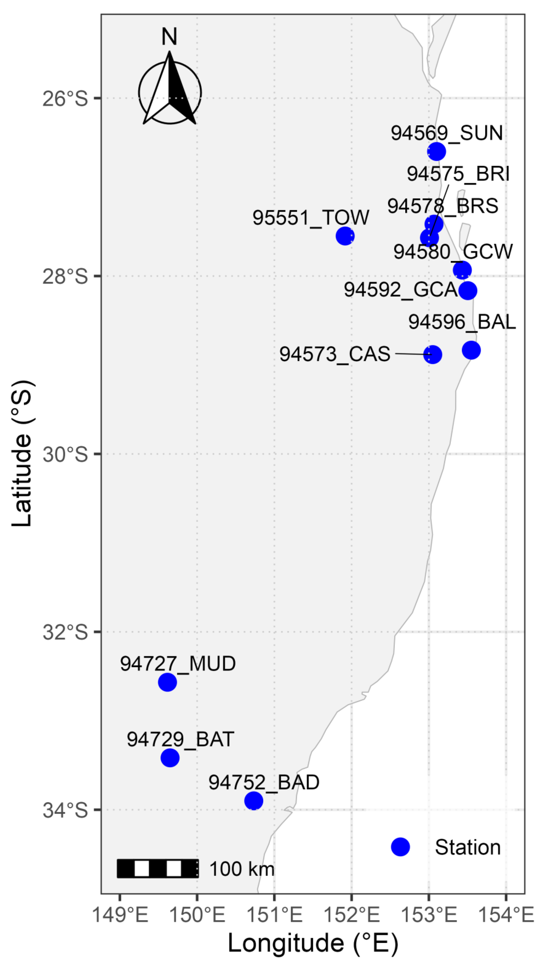
This research aims to fill this knowledge gap by conducting a comprehensive comparative analysis of BART, GPR, and QRF for probabilistic wind speed forecasting across eleven stations in NSW and QLD, Australia [37]. The study leverages 21 years (2000–2020) of daily observations, including maximum and minimum temperature, precipitation, and surface pressure, which are key meteorological drivers, to train and validate models in both at-site and regional pooling regimes. Forecasts are assessed using multiple point and probabilistic metrics: RMSE, mean absolute error (MAE), coefficient of determination (R²), bias, Pearson correlation, interval coverage, and CRPS. This multidimensional evaluation framework enables robust assessment across accuracy, calibration, and sharpness dimensions. By systematically examining performance trade-offs, spatial information transfer, and uncertainty calibration, this work advances knowledge on machine learning-based wind forecasting and informs climate-resilient energy planning.

The specific objectives are as follows: (1) to compare the point accuracy and probabilistic skill of BART, GPR, and QRF under at-site and regional modelling frameworks; (2) to quantify the impact of regional pooling on RMSE, MAE, R², bias, Pearson correlation, CRPS, and interval coverage for each method; (3) to identify key meteorological and spatial predictors through variable importance analyses; (4) to provide actionable recommendations for operational deployment in heterogeneous climatic regions; and (5) to establish benchmarks for future probabilistic wind forecasting research in Australia and beyond. These objectives are highly relevant to renewable energy sectors worldwide.

The remainder of the paper is organised as follows. Section 2 describes the study area, data sources, quality control procedures, and pre-processing steps. Section 3 details the modelling approaches, forecast generation procedures, and evaluation metrics, including the mathematical formulations for all statistical measures. Section 4 presents and discusses the results, highlighting the practical implications for energy system integration and climate adaptation. Finally, Section 5 synthesises the key findings, outlines the methodological limitations, and proposes directions for future research, including hierarchical pooling frameworks, real-time recalibration strategies, and integration with climate projection ensembles.

2. Study Area and Data

2.1. Study Region

The analysis focuses on eleven synoptically and topographically diverse meteorological stations across New South Wales (NSW) and Queensland (QLD), Australia (Figure 1). Station elevations range from 2 m (94596_BAL) to 745 m (94729_BAT), latitudes span 25.5° S–33.9° S, and longitudes cover 149.6° E–153.6° E. Coastal sites (94569_SUN, 94580_GCW) experience diurnal sea-breeze regimes, while highland stations (94727_MUD, 94729_BAT, 95551_TOW) undergo enhanced synoptic forcing, downslope winds, and mountain–valley circulations. Intermediate riverine and urban peripheral sites (94573_CAS, 94575_BRI, 94578_BRS, 94592_GCA, 94596_BAL, 94752_BAD) capture mixed microclimates shaped by land use and topography. These spatial clusters enable rigorous evaluation of regional pooling versus at-site modelling across subtropical to warm-temperate climate zones.

2.2. Data Description and Quality Control

Observed wind speed and covariates were sourced from eleven Australian Bureau of Meteorology (BoM) stations all adhering to the World Meteorological Organisation (WMO) and AS/NZS 3580.14:2014 [38] protocols for consistency. Measurements were taken at a standard 10 m height for comparability. Daily records for 1 January 2000–31 December 2020 were obtained for the following:

• Wind speed (m/s);
• Maximum temperature (°C);
• Minimum temperature (°C);
• Precipitation (mm);
• Surface pressure (hPa);
• Day of year (1–366);
• Calendar year (2000–2020);
• Station latitude (°), longitude (°), and elevation (m);
• Wind direction and large-scale climate indices (e.g., ENSO phases, SAM) were not included because these variables are not available or quality controlled at all stations on a consistent daily basis and, in some cases, require additional reanalysis processing. In this study, we deliberately restrict attention to a core set of routinely recorded BoM predictors to benchmark at-site versus regional probabilistic methods.

The quality control steps were as follows:

• Remove negative or implausible values (e.g., precipitation < 0 mm flagged).
• Ensure minimum temperature ≤ maximum temperature.
• Flag outliers beyond ±3 SD of station climatology.
• Impute isolated missing entries (<2% per station) via nearest-neighbour temporal interpolation, preserving the observed distributional properties of the original data.
• Standardisation and temporal aggregation: Following complete data interpolation, all variables (wind speed, temperature, pressure, and precipitation) were standardised to zero mean and unit variance within each modelling framework (at-site models standardised using station-specific summary statistics; regional models standardised using pooled statistics across all eleven stations). This ordering, interpolation before standardisation, ensures that imputed values respect the original data distribution and temporal patterns before transformation. It also avoids artificial bias in subsequent standardisation scaling.

The ±3 SD threshold for outlier flagging was selected as a conservative criterion balancing the need to remove implausible instrument errors while preserving meteorologically valid extremes. For wind speed, the ±3 SD criterion spans approximately ±7–8 m/s around station means (

Table 1. (a) Wind speed, elevation, and precipitation variables. (b) Temperature and pressure statistics by station.

(a)
Site ID	Elevation (m)	Mean WS (m/s)	SD WS (m/s)	Skew WS	CV WS (%)	Min WS (m/s)	Max WS (m/s)	Mean Precip (mm)	SD Precip (mm)	Skew Precip	CV Precip (%)	Max Precip (mm)
94569_SUN	4	8.89	3.03	0.84	34.05	1.4	28.8	0.16	0.5	6.63	315.94	9.13
94573_CAS	22	5.57	1.97	0.89	35.4	0.1	17.5	0.11	0.38	7.65	345.37	7.4
94575_BRI	19.2	6.79	2.21	0.7	32.59	0.6	25.1	0.1	0.36	7.72	378.01	6.34
94578_BRS	6	8.1	2.35	1.16	28.97	1.9	27	0.1	0.37	7.11	358.67	6.69
94580_GCW	3	10.39	3.8	1.19	36.61	1.1	33.2	0.13	0.5	9.42	379.62	13.81
94592_GCA	6.4	8.26	2.71	0.67	32.77	1.5	27.1	0.16	0.56	8.86	353.48	14.53
94596_BAL	2	7.36	3.08	0.5	41.75	0.2	23.3	0.19	0.56	6.25	300.73	8.55
94727_MUD	472	6.01	2.55	0.81	42.43	0.1	19.9	0.07	0.25	7.48	359.67	6.85
94729_BAT	745	6.35	2.71	0.7	42.63	0.1	19.9	0.07	0.21	5.41	317.41	2.93
94752_BAD	82	5.46	2.44	1.14	44.69	0.4	17.3	0.08	0.28	9.05	377.18	7.87
95551_TOW	642	10.86	3.39	0.53	31.23	2.9	29.7	0.08	0.38	14.36	469.26	9
(b)
Site ID	Mean Max Temp (°C)	SD Max Temp (°C)	Skew Max Temp	CV Max Temp (%)	Mean Min Temp (°C)	SD Min Temp (°C)	Skew Min Temp	CV Min Temp (%)	Mean Pressure (hPa)	SD Pressure (hpa)	Skew Pressure	CV Pressure (%)
94569_SUN	25.34	3.45	0	13.61	15.13	5.27	−0.43	34.86	1016.55	5.09	−0.15	0.5
94573_CAS	26.14	4.81	0.31	18.42	12.5	5.49	−0.22	43.92	1016.89	5.75	−0.06	0.57
94575_BRI	26.5	4	−0.02	15.11	14.07	5.35	−0.22	38.02	1016.76	5.31	−0.11	0.52
94578_BRS	25.54	3.42	−0.06	13.4	15.01	5.1	−0.27	33.99	1016.18	8.54	−0.05	0.84
94580_GCW	25.6	3.49	0.04	13.63	16.67	4.27	−0.35	25.6	1016.77	5.33	−0.12	0.52
94592_GCA	25.02	3.29	−0.06	13.15	15.17	5.04	−0.51	33.22	1015.9	9	−0.08	0.89
94596_BAL	24.53	3.77	0.08	15.38	13.76	5	−0.24	36.33	1017.05	5.6	−0.11	0.55
94727_MUD	22.82	6.89	0.22	30.17	7.33	6.68	0.05	91.13	1017.37	6.42	0.02	0.63
94729_BAT	20.77	7.09	0.22	34.14	5.91	5.92	0.14	100.19	1017.49	6.61	0.02	0.65
94752_BAD	23.87	5.82	0.56	24.39	10.09	5.63	−0.08	55.77	1017.25	6.74	−0.1	0.66
95551_TOW	23.06	5.23	0.08	22.67	12.11	4.8	−0.39	39.67	1017.25	5.36	−0.05	0.53

WS = wind speed; SD = standard deviation; CV = coefficient of variation; Precip = precipitation; Temp = temperature; SD = standard deviation; CV = coefficient of variation.

a), encompassing all observed maxima (range: 17.3–33.2 m/s). The highest wind speed recorded (33.2 m/s at 94580_GCW, a coastal site) lies within 2.3 SD of that station’s mean, confirming that genuine extreme winds from East Coast Lows and gale force events are retained by our threshold. In comparison, precipitation shows greater variability (CV = 300–469%), and the ±3 SD threshold may flag only the most extreme single-day totals (>95th percentile), which is appropriate given that occasional precipitation events can be physically implausible (e.g., daily totals exceeding 100 mm during dry seasons). This approach aligns with World Meteorological Organisation (WMO) quality standards (Australian Bureau of Meteorology, AS/NZS 3580.14:2014), which permit the retention of data flagged as physically plausible by metadata audits and historical records. Our implementation prioritises the preservation of tail behaviour which is essential for probabilistic model training over the aggressive smoothing of extremes, ensuring that quantile regression models (particularly QRF) are exposed to genuine extreme events necessary for reliable tail quantile estimation.

Interpolation and Standardisation Workflow

Temporal interpolation was applied to isolated missing observations using nearest-neighbour methods within each station’s time series prior to any standardisation. This approach preserves the observed climatological distribution and prevents artificially inflated or deflated variance estimates. Standardisation was then applied to the complete, interpolated dataset, with summary statistics (mean, standard deviation) computed separately for each station in at-site models and across all pooled observations in regional models. By maintaining this sequence (interpolation → standardisation), we ensure that imputed values do not artificially constrain variance estimates or introduce numerical artefacts that could bias model learning.

2.3. Summary Statistics

Table 1a,b presents comprehensive per-station distributional statistics for all meteorological and spatial–temporal predictors, revealing substantial environmental heterogeneity that motivates both at-site and regional modelling approaches. Coastal stations generally exhibit higher mean wind speeds and lower skewness than some inland and highland sites, indicating distinct local regimes. Precipitation and elevation also vary widely, supporting the need to examine both at-site and regional frameworks rather than assuming homogeneous behaviour.

Mean wind speeds vary by roughly a factor of two across stations, from about 5.5 m/s at sheltered inland sites to over 10.5 m/s at exposed elevated and coastal locations, with standard deviations scaling proportionally. Coastal stations generally exhibit higher means and moderate coefficients of variation, reflecting persistent onshore flow and maritime moderation, whereas elevated inland sites show the highest relative variability, indicating stronger temporal volatility. All stations display positively skewed wind speed distributions with occasional gale force events, confirming the need for probabilistic methods that capture upper tail behaviour rather than only optimising mean squared error.

Daily precipitation has low means but extremely high coefficients of variation (exceeding 300% at all stations), consistent with a zero inflated regime where infrequent heavy events dominate totals. Strong right skewness and heavy tails in precipitation highlight the importance of models that remain robust to outliers and highly skewed predictors, while the weak correlations between precipitation and other variables indicate that intense rainfall events often occur under synoptic configurations distinct from typical wind regimes.

Maximum and minimum temperatures show expected spatial patterns: coastal and low elevation sites are warmer on average, with relatively low skewness, whereas high elevation stations exhibit cooler means and higher relative variability, especially at night. These temperature patterns, together with day of year and calendar year predictors, allow the models to learn seasonal cycles and potential long-term changes in wind climatology without imposing rigid parametric forms. Surface pressure varies little in mean across stations but captures synoptic-scale variability, and, together with latitude and longitude, serves as a key driver and spatial indicator for learning location-specific wind responses.

2.4. Variable Relationships

Figure 2 displays the pairwise correlation matrix and marginal distributions for all study predictors and the wind speed target, based on 10,000 pooled observations. The upper panels show Pearson correlation coefficients, the lower panels display scatterplots, and the diagonal panels give smoothed kernel densities. The relationships observed in Figure 2 provide critical context for model selection and interpretation.

2.4.1. Wind Speed Relationships

Wind speed exhibits notably weak correlations with most predictors. The largest associations are with latitude (r = 0.35), longitude (r = 0.23), and minimum temperature (r = 0.35). The positive correlation with latitude and longitude reflects geographic gradients in wind climatology, with higher winds typically observed at more exposed coastal and/or elevated sites. The relationship with minimum temperature (r = 0.35) may reflect shared seasonal or synoptic drivers, as wind events often coincide with colder night time air masses in certain regions. Correlations with maximum temperature (r = 0.12), precipitation (r = 0.11), and pressure (r = −0.15) are modest, indicating that wind speed exhibits substantial independence from single-day values of these covariates in this multi-site context.

2.4.2. Temperature and Pressure

Maximum and minimum temperature have a strong positive association (r = 0.72), reflecting shared controls from surface energy balance and seasonal cycles. Both form moderate positive relationships with longitude and latitude, consistent with spatial gradients in temperature, while pressure demonstrates moderate negative correlations with both temperature variables (r = −0.39 with MaxTemp, r = −0.33 with MinTemp). This matches the expectation that high-pressure states are typically associated with cooler, more stable atmospheric conditions.

2.4.3. Precipitation and Temporal Predictors

Precipitation correlations with other variables are all weak (|r| < 0.11). The event-driven, zero-inflated, and highly skewed nature of daily precipitation limits its direct association with other meteorological predictors, at least in marginal relationships. This underscores the importance of modelling precipitation (and its impacts on wind) using approaches robust to heavy tails and nonlinearities. The day of year (DOY) demonstrates negligible correlation with wind speed, temperature, or pressure in this pooled analysis, but its density plot is uniform as expected, allowing models to detect cyclical annual patterns if present. The year is uncorrelated with all primary meteorological variables, as expected from an equally weighted, continuous time series spanning 2000–2020.

2.4.4. Spatial Structure and Predictor Characteristics

Latitude and longitude are strongly correlated (r = 0.87), indicating southeast coastal clustering and a northeast–southwest environmental gradient (Figure 1). Elevation correlates moderately with latitude (r = 0.46) due to southward terrain rise toward the Great Dividing Range, and negatively with temperature (r = −0.42 to −0.29) via orographic lapse-rate effects. The strong negative correlation between elevation and longitude (r = −0.79) indicates that inland elevated sites lie westward of coastal stations. Wind speed and precipitation exhibit right-skew with extreme tails; temperatures and pressure are near-Gaussian. These spatial variables enable regional models to learn continuous wind climatologies and differentiate microclimates. Weak to moderate inter-variable correlations indicate that multivariate models must account for nonlinearity and interactions while benefiting from low multicollinearity. Spatial wind associations validate hierarchical and regional approaches that pool strength across locations.

3. Methodology

3.1. Forecasting Objective and Notation

The study addresses probabilistic daily forecasting of near-surface wind speed at multiple meteorological stations across New South Wales and Queensland, Australia. Each observation comprises a predictor vector ${\mathrm{x}}_i$ containing meteorological variables (maximum temperature, minimum temperature, precipitation, surface pressure), temporal features (day of year, calendar year), and site attributes (latitude, longitude, elevation), together with the target wind speed y_i. The probabilistic forecasting objective is to estimate the conditional predictive distribution $P\left(Y∣{\mathrm{x}}_{*}\right)$ for a new input x_∗, from which the following are derived:

• Point forecasts: Posterior predictive mean $\mathbb{E}\left[Y∣{\mathrm{x}}_{*}\right] \mathrm{a}\mathrm{n}\mathrm{d} \mathrm{m}\mathrm{e}\mathrm{d}\mathrm{i}\mathrm{a}\mathrm{n} \mathrm{m}\mathrm{e}\mathrm{d} \left[Y∣{\mathrm{x}}_{*}\right]$.
• Interval forecasts: Central (1 − α) prediction interval endpoints ${\widehat{q}}_{\alpha /2}({\mathrm{x}}_{*})$ and ${\widehat{q}}_{1-\alpha /2}({\mathrm{x}}_{*})$.
• Probabilistic scores: Continuous Ranked Probability Score (CRPS), coverage probability, and interval sharpness.

These outputs support comprehensive uncertainty quantification, calibration evaluation, and risk-sensitive operational decision-making for renewable energy integration and grid management.

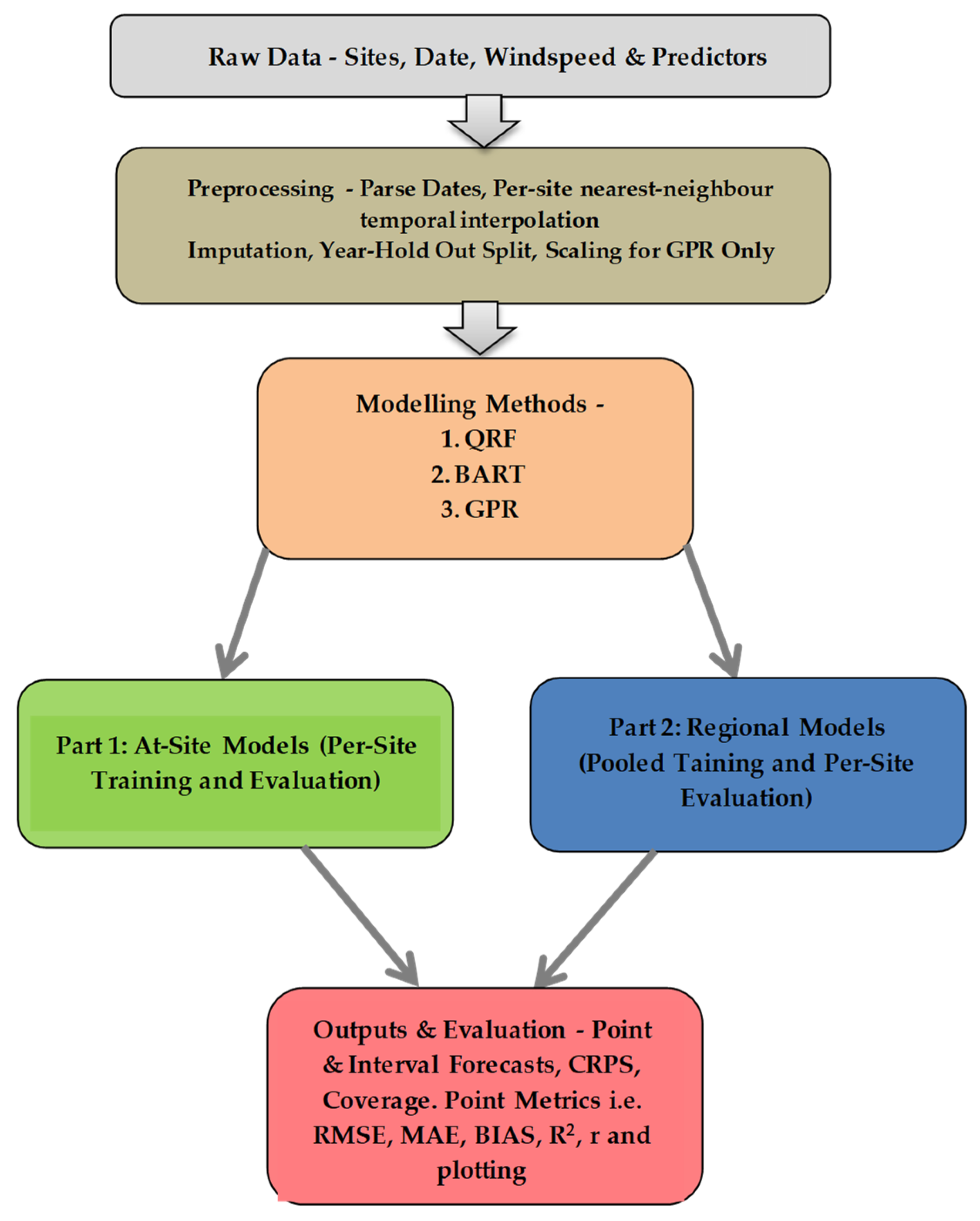
A strict year-based holdout strategy is employed to ensure temporal separation and realistic evaluation. The dataset is partitioned into training (years 2000–Y − 1) and testing (year Y) subsets, where Y represents a single held-out year. The workflow is illustrated in Figure 3, which outlines the progression from data pre-processing to model training, prediction, and evaluation. Three fundamental assumptions underpin the methodology:

• Predictor–target relationships remain approximately stationary over the 21-year study period, with any nonstationarity captured through the inclusion of temporal trend predictors (year, cyclical day of year). Here, the “year” covariate serves as a simple, low dimensional proxy for gradual climate-driven changes over 2000–2020, and we regard more complex dynamic or regime switching treatments of nonstationarity as an important but separate extension beyond the scope of this benchmark comparison.
• All primary drivers of short-term wind variability are represented in the selected predictor set, informed by established meteorological theory and variable importance analyses.
• Temporal leakage is rigorously prevented by maintaining strict chronological separation between training and test data, with no future information available during model fitting or hyperparameter tuning.

3.2. Modelling Strategy: At-Site Versus Regional Frameworks

The analysis evaluates two complementary modelling regimes designed to test alternative strategies for leveraging spatial information (Figure 3).

3.2.1. At-Site Modelling

Independent models are trained for each station using only its local historical record. This approach maximises fidelity to site-specific climatology, capturing microclimatic idiosyncrasies, local topographic effects, and station-specific predictor–wind relationships. However, at-site models may suffer from limited sample sizes when estimating rare extreme events (e.g., gale force winds from East Coast Lows), potentially leading to wider prediction intervals and reduced skill for tail quantiles.

3.2.2. Regional (Pooled) Modelling

A single model trained on pooled observations from all eleven stations includes station metadata (latitude, longitude, elevation) as predictors, enabling spatial transferability. Regional pooling increases sample size for extreme events, potentially improving prediction intervals. However, spatial predictors may miss microclimatic signals. Both frameworks use identical algorithms, predictors, and tuning to ensure comparability. Performance differences reveal trade-offs between site-specific precision and pooled information sharing, directly addressing whether regional models yield forecast improvements.

3.3. Probabilistic Machine Learning Algorithms

Three state-of-the-art probabilistic machine learning methods are implemented.

3.3.1. Quantile Regression Forests (QRF)

Quantile Regression Forests (QRF) extends the random forest algorithm to estimate conditional quantiles by retaining all terminal node observations rather than computing node means. The ensemble-aggregated empirical cumulative distribution function (CDF) is

$$\widehat{F}=\left(\xi |{\mathrm{x}}_{*}\right)={\displaystyle \frac{1}{T}}\sum _{t=1}^T{\displaystyle \frac{{\sum }_{i\in {\mathrm{l}\mathrm{e}\mathrm{a}\mathrm{f}}_t\left({\mathbf{x}}_{*}\right)}1\left\{y_i\le \xi \right\}}{\left|{\mathrm{l}\mathrm{e}\mathrm{a}\mathrm{f}}_t\left({\mathrm{x}}_{*}\right)\right|}},$$

(1)

where T is the number of trees. Quantiles at any level τ ∈ (0, 1) are obtained by

$${\widehat{q}}_{\tau }\left({\mathrm{x}}_{*}\right)=inf\left\{\xi :\widehat{F}=\left(\xi |{\mathrm{x}}_{*}\right)\ge \tau \right\}.$$

(2)

Predictive medians (τ = 0.5), 95% prediction intervals (τ = 0.025, 0.975), and CRPS are computed directly from $\widehat{F}$. QRF naturally accommodates nonlinear predictor interactions, conditional heteroskedasticity, and non-Gaussian response distributions without parametric assumptions. Key hyperparameters—number of trees, minimum terminal node size, and number of variables randomly sampled per split—are tuned via nested cross-validation to optimise mean CRPS on validation folds. While QRF is highly flexible, its reliance on empirical order statistics can make extreme quantiles less stable and contributes to the under-coverage behaviour discussed in Section 4.3.

3.3.2. Bayesian Additive Regression Trees (BART)

BART represents the regression function as an ensemble sum of many weakly regularised regression trees:

$$f\left(x\right)= \sum _{j=1}^{m}g\left(\mathrm{x}; T_j, M_j\right),$$

(3)

where each tree T_j partitions the input space into terminal regions, and $M_j={\left\{{\mu }_{j,\mathcal{l}}\right\}}_{\mathcal{l}=1}^{L_j}$ assigns a scalar leaf parameter to each terminal node. Bayesian priors are placed on tree structures (favouring shallow trees via a depth-penalising prior), splitting rules (uniform over available predictors and split points), and leaf parameters (Gaussian with small variance to encourage weak learners). The observational model is

$$y_i=f\left({\mathrm{x}}_i\right)+{ϵ}_i, {ϵ}_i\sim N\left(0,{\sigma }^2\right),$$

(4)

with a conjugate inverse-gamma prior on σ². Posterior inference is conducted via Bayesian back fitting MCMC, iteratively updating each tree conditional on the residuals from all others, yielding posterior samples ${\left\{f^{\left(s\right)}\left(\mathbf{x}\right),{\sigma }^{2\left(s\right)}\right\}}_{s=1}^S.$ Predictive distributions are obtained by drawing

$${\tilde{y}}^{\left(s\right)}\sim N\left(f^{\left(s\right)}\left({\mathrm{x}}_{*}\right),{\sigma }^{2\left(s\right)}\right),$$

(5)

from which posterior predictive quantiles, means, and variances are computed empirically. BART’s sum-of-trees structure and regularisation priors enable flexible nonlinear modelling while avoiding overfitting, making it well-suited for heterogeneous spatial data. Hyperparameters (number of trees m, tree depth prior parameters, and leaf variance prior scale) are tuned to balance computational cost, posterior mixing, and out-of-sample predictive performance.

3.3.3. Gaussian Process Regression (GPR)

GPR is a kernel-based nonparametric Bayesian method that places a Gaussian process prior on the latent regression function f(x), assuming that observations arise from

$$y=f\left(\mathrm{x}\right)+ϵ,ϵ\sim N\left(0,{\sigma }_n^2\right),$$

(6)

where $f~\mathcal{G}\mathcal{P}\left(0, k(.,.\right)) \mathrm{a}\mathrm{n}\mathrm{d} k\left(\mathrm{x},{\mathrm{x}}^{\prime }\right)$ is a positive-definite covariance (kernel) function encoding prior beliefs about function smoothness and length scales. We employ the squared exponential (radial basis function) kernel with automatic relevance determination (ARD):

$$k\left(\mathrm{x},{\mathrm{x}}^{\mathbf{\prime }}\right)= {\sigma }_f^2\exp \left(-{\displaystyle \frac{1}{2}}\sum _{d=1}^p{\displaystyle \frac{{{(x}_d-x_d^{\prime })}^2}{{\mathcal{l}}_d^2}}\right),$$

(7)

where ${\sigma }_f^2$ controls signal variance and ${\left\{{\mathcal{l}}_d\right\} }_{d=1}^p$ are predictor-specific length scales governing smoothness along each dimension. Given training inputs X and observations y, the posterior predictive distribution at ${\mathrm{x}}_{*}$ is Gaussian with closed-form mean and variance:

$${\mu }_{*\left({\mathbf{x}}_{*}\right)}= {\mathrm{k}}_{*}^{\mathrm{T}}{\left(K+{\sigma }_n^{2}I\right)}^{-1}\mathrm{y}, {\sigma }_{*}^2\left({\mathrm{x}}_{*}\right)=k\left({\mathrm{x}}_{*},{\mathrm{x}}_{*}\right)- {\mathrm{k}}_{*}^{\mathrm{T}}{\left(K+{\sigma }_n^{2}I\right)}^{-1}{\mathrm{k}}_{*},$$

(8)

where K is the n × n training covariance matrix, ${\mathrm{k}}_{*}={\left[k\left({\mathrm{x}}_i,{\mathrm{x}}_{*}\right)\right]}_{i=1}^n$, and ${\sigma }_n^2$ is the observation noise variance. Prediction intervals are constructed from the Gaussian predictive distribution $N=\left(\mu \left({\mathrm{x}}_{*}\right),{\sigma }^2\left({\mathrm{x}}_{*}\right)\right)$.

Kernel hyperparameters {${\mathcal{l}}_d, {\sigma }_f^2,{\sigma }_n^2$} are optimised by maximising the marginal log-likelihood on a representative subsample of training data (up to 2000 points selected to preserve distributional characteristics), ensuring computational tractability for large datasets while maintaining predictive accuracy. GPR’s analytic predictive variance provides interpretable epistemic uncertainty estimates, revealing regions of input space with limited training coverage or high intrinsic variability.

3.4. Performance Metrics

Forecast performance is evaluated using a comprehensive suite of deterministic and probabilistic metrics, each designed to assess distinct aspects of forecast quality. Deterministic metrics characterise point forecast accuracy, while probabilistic metrics evaluate the full predictive distribution’s calibration, sharpness, and reliability. Together, these metrics provide a holistic assessment of operational forecast utility across varying risk tolerance and decision contexts.

3.4.1. Deterministic Point Forecast Metrics

Root Mean Squared Error (RMSE):

$$\mathrm{R}\mathrm{M}\mathrm{S}\mathrm{E}=\sqrt{{\displaystyle \frac{1}{n}}\sum _{i=1}^n{\left(y_i-{\widehat{y}}_i\right)}^2},$$

(9)

where ${\widehat{y}}_i=\mathbb{E}\left[Y∣{\mathbf{x}}_i\right]$ is the posterior predictive mean. RMSE quantifies the average magnitude of forecast errors with heavier penalties for large deviations, making it sensitive to outliers and extreme events. It is widely used in energy forecasting benchmarks but can be misleading when extreme events are rare, as squared errors from a few outliers may dominate the metric. Lower RMSE indicates better point forecast accuracy.

Mean Absolute Error (MAE):

$$\mathrm{M}\mathrm{A}\mathrm{E}={\displaystyle \frac{1}{n}}\sum _{i=1}^n\left|y_i-{\widehat{y}}_i\right|,$$

(10)

MAE measures average forecast error magnitude with equal weighting across all observations, providing robustness to outliers compared to RMSE. It is interpretable in the original units of wind speed (m/s) and reflects typical day-to-day forecast performance. MAE is preferred when operational costs scale linearly with forecast error rather than quadratically.

Coefficient of Determination ($R^2$):

$$R^2=1-{\displaystyle \frac{{\sum }_{i=1}^n{\left(y_i-{\widehat{y}}_i\right)}^2}{{\sum }_{i=1}^n{\left(y_i-\overline{y}\right)}^2}},$$

(11)

Here, $y_i$ and ${\widehat{y}}_i$ denote observed and predicted wind speed at time i, respectively, and $\overline{y}$ is the mean of the observed wind speeds over the evaluation set. $R^2$ quantifies the proportion of variance in observed wind speed explained by the model, ranging from −∞ to 1. Values near 1 indicate high explanatory power, while negative values suggest that the model performs worse than a naive mean-based climatology. $R^2$ provides a scale-free measure of goodness-of-fit but can be inflated by temporal autocorrelation in time series data.

Bias:

$$\mathrm{B}\mathrm{i}\mathrm{a}\mathrm{s}={\displaystyle \frac{1}{n}}\sum _{i=1}^n\left({\widehat{y}}_i-y_i\right).$$

(12)

Bias measures systematic over- or under-prediction. Zero bias indicates unbiased forecasts (symmetric errors), while positive or negative bias reveals directional forecast tendencies.

Pearson Correlation Coefficient (r):

$$r={\displaystyle \frac{{\sum }_{i=1}^n\left(y_i-\overline{y}\right)\left({\widehat{y}}_i-\overline{\widehat{y}}\right)}{\sqrt{\sum _{i=1}^n{\left(y_i-\overline{y}\right)}^2}\sqrt{\sum _{i=1}^n{\left({\widehat{y}}_i-\overline{\widehat{y}}\right)}^2}}}$$

(13)

The correlation coefficient measures the linear association between observed and predicted wind speeds, ranging from −1 to 1. High positive correlation indicates that the model successfully captures temporal patterns and variability phasing, even if absolute magnitudes may differ due to bias or scaling issues. Correlation is particularly useful when evaluating trend-following skill independent of bias.

3.4.2. Probabilistic Forecast Metrics

Prediction Interval Coverage Probability (PICP):

$${\mathrm{P}\mathrm{I}\mathrm{C}\mathrm{P}}_{1-\alpha }= {\displaystyle \frac{1}{n}}\sum _{\left\{i=1\right\}}^{n}1\left\{{\widehat{q}}_{\alpha /2}\left({\mathrm{x}}_i\right)\le y_i\le {\widehat{q}}_{1-\alpha /2}\left({\mathrm{x}}_i\right)\right\},$$

(14)

where ${\widehat{q}}_{\alpha /2}$ and ${\widehat{q}}_{1-\alpha /2}$ are the estimated lower and upper quantiles of the predictive distribution, and 1{⋅} is the indicator function. PICP assesses calibration by comparing empirical coverage to the nominal level 1 − α. Well-calibrated forecasts achieve PICP ≈ 1 − α (e.g., 95% intervals should contain the observation ~95% of the time). Under-coverage (PICP < 1 − α) indicates overly narrow, overconfident intervals that fail to capture true uncertainty, leading to increased operational risk. Over-coverage (PICP > 1 − α) suggests excessively wide, conservative intervals that may be unhelpful for decision-making despite being formally valid.

Continuous Ranked Probability Score (CRPS):

We evaluate probabilistic forecasts with metrics and graphical diagnostics that assess both calibration and sharpness. One such metric is the Continuous Ranked Probability Score (CRPS) [39]. For a predictive CDF F and observed value y,

$$\mathrm{C}\mathrm{R}\mathrm{P}\mathrm{S}(F,y)={\int }_{-\infty }^{\infty }{\left(F\left(z\right)-1\left\{z\ge y\right\}\right)}^{2}dz$$

(15)

where F is the predictive cumulative distribution function and y the observation. CRPS is a strictly proper scoring rule that simultaneously rewards calibration and sharpness: well-calibrated forecasts with narrow predictive distributions achieve lower CRPS. Unlike RMSE, which evaluates only the predictive mean, CRPS penalises the entire predictive distribution’s deviation from the observed outcome, making it the gold standard for probabilistic forecast evaluation. For sample-based distributions (QRF, BART), CRPS is computed via

$${\mathrm{C}\mathrm{R}\mathrm{P}\mathrm{S}}_{\mathrm{e}\mathrm{m}\mathrm{p}\mathrm{e}\mathrm{r}\mathrm{i}\mathrm{c}\mathrm{a}\mathrm{l}}={\displaystyle \frac{1}{M}}\sum _{m=1}^M\left|y-{\tilde{y}}_m\right|-{\displaystyle \frac{1}{2M^2}}\sum _{m=1}^M\sum _{m^{\prime }=1}^M\left|{\tilde{y}}_m-{\tilde{y}}_{m^{\prime }}\right|,$$

(16)

where ${\left\{{\tilde{y}}_m\right\}}_{m=1}^M$ are predictive samples. For Gaussian predictive distributions (GPR), the analytic form is

$$\mathrm{C}\mathrm{R}\mathrm{P}\mathrm{S}\left(N\left(\mu ,{\sigma }^2\right),y\right)=\sigma \left[z\left(2\mathsf{\Phi }\left(z\right)-1\right)+2\varphi \left(z\right)-{\displaystyle \frac{1}{\sqrt{\pi }}}\right], z={\displaystyle \frac{y-\mu }{\sigma }},$$

(17)

where Φ and ϕ are the standard normal cumulative distribution function (CDF) and probability distribution function (PDF). Lower CRPS indicates superior probabilistic forecast quality, combining accuracy, calibration, and sharpness in a single metric interpretable in units of wind speed (m/s).

3.4.3. Joint Interpretation and Complementarity

No single metric captures all forecast dimensions. RMSE and MAE assess point accuracy; R² and correlation measure pattern-matching and variance explanation. PICP evaluates calibration without penalising wide intervals. CRPS uniquely integrates accuracy, calibration, and sharpness, serving as the primary probabilistic metric. Bias detection informs post-processing; correlation confirms temporal phasing. Evaluating models across this comprehensive suite ensures that improvements in one dimension—e.g., narrower intervals via regional pooling—do not compromise others like calibration, supporting robust conclusions about operational utility.

3.5. Variable Importance and Interpretability

Variable importance is assessed for QRF, BART, and GPR using method-specific, normalised metrics. QRF uses permutation-based CRPS degradation; BART derives importance from posterior tree-split frequencies; GPR employs permutation analogous to QRF. Comparing at-site versus regional patterns reveals trade-offs: regional models leverage spatial predictors for cross-site pooling, while at-site models rely on local conditions for microclimatic fidelity. This validates physical plausibility, informs operational feature selection for efficiency, and identifies hybrid modelling opportunities. Variable importance is visualised via bar plots across all sites, algorithms, and frameworks, providing interpretable insights into wind forecast drivers across Australian environments.

3.6. Cross-Validation, Hyperparameter Tuning, and Implementation

A strict year-based holdout strategy ensures temporal separation and realistic forecast evaluation, as illustrated in Figure 3. Data are partitioned into training (years 2000 to Y − 1) and testing (year Y) subsets, where Y represents a single held-out year. This approach mirrors operational forecasting scenarios where models trained on historical records must predict an entire future year without access to contemporaneous observations, thereby preventing temporal leakage and look-ahead bias.

Hyperparameter tuning is conducted exclusively within the training partition via nested five-fold cross-validation, optimising average CRPS on validation folds. For QRF, key hyperparameters include the number of trees (100, 500, 1000), minimum terminal node size (5, 10, 20), and the number of variables randomly sampled per split (√p, p/3, p/2). For BART, tuning focuses on the number of trees in the ensemble (50, 200, and 500), tree depth prior parameters controlling split probabilities, the leaf variance prior scale, and the number of post burn-in MCMC iterations (1000–5000). For GPR, hyperparameters include kernel selection (squared exponential with automatic relevance determination), predictor-specific length scale priors (log normal), and observation noise variance priors (inverse-gamma). To maintain computational tractability, GPR hyperparameters are optimised on a stratified 2000 observation subsample that preserves the joint distribution of predictors and responses, and the resulting configuration is applied when predicting for the full test set. Once optimal hyperparameters are identified, final models are refit on the complete training dataset before generating forecasts for the held-out test year. All comparisons reflect genuine out-of-sample performance under strict temporal ordering. Models are implemented in R (version 4.5) [40], using ranger (QRF) [41], dbarts (BART) [22,42], and kernlab/GPfit (GPR) [43,44].

4. Results and Discussion

4.1. Overview and Evaluation Framework

This section presents a comprehensive, multidimensional comparison of Quantile Regression Forests (QRF), Bayesian Additive Regression Trees (BART), and Gaussian Process Regression (GPR) under both at-site and regional modelling frameworks across eleven meteorological stations in NSW and QLD, Australia. Performance is evaluated using strict year-based holdout validation across seven complementary metrics: RMSE and MAE for point forecast accuracy, R² and correlation (r) for variance explanation and pattern matching, bias for systematic error detection, coverage for interval calibration, and CRPS for integrated probabilistic skill. Results are presented at both the individual site level (

Table 2. (a) Comprehensive per-site performance metrics (at-site, all 11 stations × 3 models). (b) Comprehensive per-site performance metrics (regional, all 11 stations × 3 models).

(a)
At-Site Modelling
Site ID	Model	RMSE	MAE	R2	BIAS	r	Coverage	CRPS
94569_SUN	QRF	2.45	1.92	0.27	0.21	0.52	0.73	1.44
94569_SUN	BART	2.51	1.96	0.25	0.14	0.5	0.95	1.4
94569_SUN	GPR	2.49	1.97	0.24	−0.03	0.49	0.98	1.36
94573_CAS	QRF	1.42	1.14	0.37	0.38	0.61	0.78	0.84
94573_CAS	BART	1.41	1.12	0.36	0.3	0.6	0.99	0.8
94573_CAS	GPR	1.43	1.15	0.36	0.39	0.6	0.97	0.8
94575_BRI	QRF	1.89	1.47	0.36	0.32	0.6	0.67	1.12
94575_BRI	BART	1.96	1.55	0.33	0.41	0.58	0.94	1.1
94575_BRI	GPR	1.93	1.51	0.32	0.2	0.57	0.96	1.07
94578_BRS	QRF	2.13	1.7	0.24	0.23	0.49	0.67	1.29
94578_BRS	BART	2.21	1.76	0.2	0.24	0.45	0.93	1.24
94578_BRS	GPR	2.22	1.74	0.17	−0.04	0.41	0.94	1.23
94580_GCW	QRF	3.53	2.85	0.13	1.48	0.35	0.62	2.14
94580_GCW	BART	3.4	2.67	0.14	1.16	0.38	0.94	1.89
94580_GCW	GPR	3.53	2.73	0.09	1.05	0.3	0.97	1.9
94592_GCA	QRF	2.46	1.92	0.2	0.46	0.44	0.69	1.45
94592_GCA	BART	2.42	1.91	0.21	0.36	0.46	0.97	1.34
94592_GCA	GPR	2.48	1.93	0.18	0.29	0.42	0.97	1.36
94596_BAL	QRF	2.66	2.07	0.22	0.19	0.47	0.69	1.56
94596_BAL	BART	2.79	2.14	0.17	0.27	0.41	0.95	1.55
94596_BAL	GPR	2.77	2.18	0.17	0.05	0.41	0.95	1.54
94727_MUD	QRF	2.27	1.82	0.34	0.68	0.58	0.7	1.37
94727_MUD	BART	2.47	2.01	0.33	1.1	0.57	0.92	1.41
94727_MUD	GPR	2.17	1.71	0.37	0.42	0.61	0.95	1.21
94729_BAT	QRF	2.07	1.67	0.41	0.17	0.64	0.71	1.25
94729_BAT	BART	2.18	1.76	0.36	0.37	0.6	0.96	1.25
94729_BAT	GPR	2.05	1.64	0.42	0.13	0.65	0.97	1.15
94752_BAD	QRF	2.05	1.63	0.34	0.45	0.59	0.72	1.22
94752_BAD	BART	2.05	1.64	0.35	0.44	0.59	0.96	1.15
94752_BAD	GPR	2.13	1.6	0.26	−0.02	0.51	0.94	1.14
95551_TOW	QRF	2.59	2.07	0.37	0.03	0.61	0.73	1.55
95551_TOW	BART	2.6	2.09	0.36	0.2	0.6	0.96	1.47
95551_TOW	GPR	2.87	2.24	0.23	−0.05	0.48	0.95	1.57
(b)
Regional Modelling
Site ID	Model	RMSE	MAE	R2	BIAS	r	Coverage	CRPS
94569_SUN	QRF	2.46	1.94	0.27	0.22	0.52	0.67	1.49
94569_SUN	BART	2.49	1.97	0.24	0.16	0.49	0.66	1.5
94569_SUN	GPR	2.64	2.09	0.16	0.13	0.39	0.94	1.46
94573_CAS	QRF	1.4	1.12	0.38	0.36	0.61	0.9	0.79
94573_CAS	BART	1.54	1.19	0.27	0.29	0.52	0.9	0.86
94573_CAS	GPR	1.99	1.48	0.16	0.85	0.4	0.99	1.06
94575_BRI	QRF	1.88	1.46	0.37	0.32	0.61	0.78	1.08
94575_BRI	BART	1.98	1.55	0.28	0.06	0.53	0.81	1.14
94575_BRI	GPR	2.22	1.78	0.16	0.48	0.4	0.97	1.23
94578_BRS	QRF	2.12	1.69	0.25	0.23	0.5	0.74	1.27
94578_BRS	BART	2.3	1.86	0.12	0.16	0.35	0.74	1.39
94578_BRS	GPR	2.58	1.9	0.03	−0.22	0.16	0.93	1.39
94580_GCW	QRF	3.56	2.85	0.11	1.45	0.33	0.45	2.33
94580_GCW	BART	3.62	2.92	0.08	1.5	0.28	0.42	2.37
94580_GCW	GPR	3.44	2.47	0.04	−0.54	0.19	0.89	1.82
94592_GCA	QRF	2.48	1.95	0.19	0.5	0.44	0.69	1.49
94592_GCA	BART	2.59	2.02	0.13	0.45	0.36	0.66	1.55
94592_GCA	GPR	2.73	2.13	0.08	0.5	0.28	0.96	1.5
94596_BAL	QRF	2.69	2.09	0.21	0.19	0.45	0.66	1.63
94596_BAL	BART	2.79	2.2	0.14	−0.11	0.37	0.59	1.72
94596_BAL	GPR	2.89	2.3	0.1	0.14	0.31	0.93	1.62
94727_MUD	QRF	2.25	1.79	0.35	0.68	0.6	0.71	1.35
94727_MUD	BART	2.3	1.84	0.34	0.74	0.58	0.72	1.38
94727_MUD	GPR	2.26	1.78	0.29	0.16	0.54	0.93	1.26
94729_BAT	QRF	2.09	1.67	0.4	0.24	0.63	0.74	1.26
94729_BAT	BART	2.27	1.83	0.32	0.38	0.56	0.71	1.38
94729_BAT	GPR	2.09	1.68	0.4	0.02	0.63	0.96	1.17
94752_BAD	QRF	2.06	1.64	0.34	0.49	0.59	0.76	1.21
94752_BAD	BART	2.11	1.68	0.31	0.54	0.56	0.76	1.25
94752_BAD	GPR	2.16	1.7	0.23	0.15	0.48	0.94	1.19
95551_TOW	QRF	2.6	2.08	0.36	0.06	0.6	0.66	1.62
95551_TOW	BART	2.71	2.18	0.3	0.24	0.55	0.62	1.69
95551_TOW	GPR	3.05	2.43	0.11	−0.11	0.33	0.95	1.72

a,b) to reveal spatial patterns and in aggregate form (

Table 3. Aggregate performance summary (mean across 11 stations, all metrics).

Metric	QRF At-Site	QRF Regional	QRF Δ	BART At-Site	BART Regional	BART Δ	GPR At-Site	GPR Regional	GPR Δ
RMSE (m/s)	2.315	2.321	+0.006	2.359	2.423	+0.064	2.364	2.544	+0.181
MAE (m/s)	1.837	1.838	+0.001	1.867	1.926	+0.058	1.849	1.971	+0.122
R2	0.290	0.289	−0.000	0.273	0.226	−0.047	0.249	0.154	−0.095
Bias (m/s)	0.416	0.425	+0.009	0.449	0.398	−0.051	0.216	0.141	−0.075
Correlation	0.531	0.530	−0.001	0.516	0.465	−0.051	0.489	0.368	−0.121
Coverage	0.697	0.701	+0.004	0.946	0.685	−0.261	0.954	0.941	−0.013
CRPS (m/s)	1.380	1.407	+0.027	1.322	1.470	+0.148	1.298	1.397	+0.099

) to identify overall behaviours and responses to regional pooling.

Table 2a,b shows that in the at-site framework, QRF, and BART achieve comparable point forecast skill, with QRF often providing slightly lower RMSE and MAE, while BART tends to deliver better interval coverage. Under regional pooling, QRF exhibits the smallest increase in RMSE, confirming its strength in point accuracy, but its coverage drops well below nominal values, indicating under-dispersed prediction intervals. In contrast, regional GPR incurs the largest RMSE penalty yet achieves the lowest CRPS and near-nominal coverage, demonstrating that it offers the most reliable probabilistic forecasts despite modest losses in point accuracy. Thus, even without an additional figure, Table 2 makes clear that QRF is preferable when deterministic accuracy is the primary objective, whereas GPR is better suited to applications where calibrated uncertainty quantification is critical. These performance differences are consistent with the weak marginal predictor–wind correlations and pronounced spatial gradients shown in Figure 2, which highlight both the limited explanatory power of any single predictor and the importance of spatial pooling across heterogeneous sites.

4.2. Point Forecast Accuracy: RMSE, MAE, and Algorithm Dominance

QRF demonstrates exceptional stability, with RMSE increasing only marginally under regional pooling and remaining virtually unchanged from the at-site baseline of 2.315 m/s (Table 3). This remarkable robustness stems from QRF’s nonparametric ensemble structure, which aggregates local empirical distributions without imposing global parametric constraints, enabling stable median forecasts despite pooling heterogeneous coastal and inland sites. BART shows moderate degradation, while GPR experiences substantial accuracy loss, the largest among all methods. Site-level analysis (Table 2) reveals that GPR’s RMSE penalty is most severe at coastal station 94573_CAS, where strong sea-breeze dynamics not represented in the inland-dominated pooled training set force the global kernel to smooth inappropriately over local microclimatic signals. QRF achieves the lowest RMSE at 6/11 sites at-site and dominates at 10/11 sites regionally, confirming its superiority for point forecast applications.

MAE patterns closely mirror RMSE but with reduced sensitivity to extreme outliers. QRF remains virtually stable, BART degrades moderately, and GPR shows larger increases. The MAE–RMSE ratio provides insight into error distribution tail behaviour: QRF and BART maintain ratios near 0.79–0.80 across regimes, indicating symmetric error distributions, while GPR’s ratio decreases slightly under pooling (0.78 → 0.77), suggesting marginally heavier tails from occasional large mispredictions at atypical sites.

4.3. Variance Explanation and Pattern Matching: R² and Correlation

All algorithms experience R² declines under pooling, with GPR suffering most severely (a 38% relative loss). This indicates that pooling introduces unexplained variance: as training data mix sites with fundamentally different wind climatologies, residual variance increases faster than models can capture through spatial predictors alone. BART’s R² drops nominally, while QRF remains nearly flat, again demonstrating its robustness to spatial heterogeneity. At station 94573_CAS, GPR’s R² collapses by −56%, confirming the severe model–environment mismatch when pooling forces global smoothing over local sea-breeze regimes.

Correlation coefficients assess temporal phasing skill independent of bias or variance scaling. QRF maintains the highest correlation (0.531 at-site, 0.530 regional), indicating a superior pattern-matching ability. BART and GPR show larger correlation declines, suggesting that pooling degrades their ability to track day-to-day wind variability phasing. This is particularly problematic for GPR, whose correlation drops to 0.368 regionally, barely above weak correlation thresholds. The strong correlation–R² relationship (both metrics rank QRF > BART > GPR) validates that forecast quality depends primarily on capturing temporal patterns rather than merely achieving low absolute errors. An important insight emerges from the comparison of Pearson correlation (r) and coefficient of determination (R²) across models. QRF consistently achieves high correlation (r ≈ 0.53–0.56 regionally), yet modest R² (~0.25–0.30), indicating strong temporal phase fidelity (timing of wind events) but weaker amplitude matching (magnitude accuracy). Mathematically, R² = r² − 2.r.bias (approximately), so for r = 0.53 to yield R² = 0.28 requires systematic bias and/or variance under-prediction. This trade-off reflects QRF’s inherent property: individual trees partition predictor space into finite regions, constraining the range of predicted values to the observed training range. Thus, QRF excels at capturing when winds will occur (phase) but struggles to predict how strong they will be (amplitude), particularly for weak and extreme wind days. Conversely, BART and GPR, through Gaussian noise and kernel-based extrapolation, respectively, can predict wind speeds beyond the training range, improving amplitude matching at the cost of occasional temporal misalignment. For operational wind forecasting, the phase–amplitude trade-off has distinct implications:

-

Energy yield estimation (cumulative power over multi-week horizons) relies primarily on amplitude matching, since under-predicting magnitudes biases cumulative generation downward. Here, BART and GPR are preferable.

-

Ramp forecasting (rapid wind speed changes) relies primarily on phase fidelity (detecting the timing of gusts or wind drops), where QRF’s high correlation is a strength.

This dichotomy clarifies why a single best model is inadvisable; instead, operational systems should deploy ensemble combinations (e.g., QRF for ramp detection, GPR for interval forecasts) or select methods based on specific use cases.

4.4. Systematic Error: Bias Assessment

All models exhibit positive mean bias, systematically over-predicting wind speeds by 0.14–0.45 m/s on average (Table 3). QRF shows the highest at-site bias, remaining nearly constant under pooling. BART’s bias actually decreases under pooling, a rare beneficial pooling effect suggesting that averaging over diverse sites mitigates site-specific over-prediction tendencies. GPR exhibits the lowest bias in both regimes, with the largest reduction, indicating that kernel smoothing over a broader spatial domain helps centre predictions closer to observations despite sacrificing R².

At high-wind station 94580_GCW, all models show severe positive bias, reflecting difficulty capturing extreme wind regimes. Remarkably, GPR’s bias at this site reverses under pooling, swinging to under-prediction as the global kernel trained on lower-wind sites systematically underestimates this location’s characteristic high winds. This dramatic bias shift, coupled with maintained coverage (0.967 → 0.884), illustrates GPR’s trade-off: inflated predictive variance preserves calibration but point forecasts drift from local climatology. At 94573_CAS, GPR’s bias explodes positively by +0.461, reinforcing site-specific pooling vulnerabilities.

4.5. Probabilistic Calibration: Coverage Collapse and Resilience

This metric reveals the starkest differences among algorithms. GPR maintains near-nominal coverage in both regimes, demonstrating robust uncertainty quantification. In contrast, BART experiences catastrophic coverage collapse by Δ = −0.261, falling 26% short of the nominal 95% level. This breakdown occurs because BART’s posterior predictive variance, governed by fixed noise priors calibrated on homogeneous at-site data, fails to expand adequately when pooling introduces high-variance coastal sites alongside low-variance inland locations. QRF shows persistent severe under-coverage at 0.70 in both regimes, indicating systematic interval under-dispersion regardless of pooling: intervals are too narrow to capture true uncertainty because local neighbourhood densities become diluted in predictor space. The under-coverage of regional QRF can be traced to its reliance on empirical order statistics in terminal nodes when estimating extreme quantiles (τ = 0.025, 0.975). In sparse regions of predictor space, effective sample sizes within leaves are small, so the upper and lower quantiles are estimated from few observations and tend to be conservative relative to the nominal 95% level, leading to systematically narrow intervals.

At station 94580_GCW, BART’s coverage plummets from 0.936 to 0.420, meaning that 58% of observations fall outside of prediction intervals—a complete calibration failure rendering forecasts operationally useless for risk management. QRF at the same site drops significantly, confirming that neither method adequately quantifies uncertainty at high-variability locations under pooling. Only GPR maintains reasonable coverage (0.967 → 0.884), though still declines nonetheless. These patterns underscore that calibration maintenance under heterogeneous pooling is GPR’s unique strength, arising from its kernel-based analytic variance inflation.

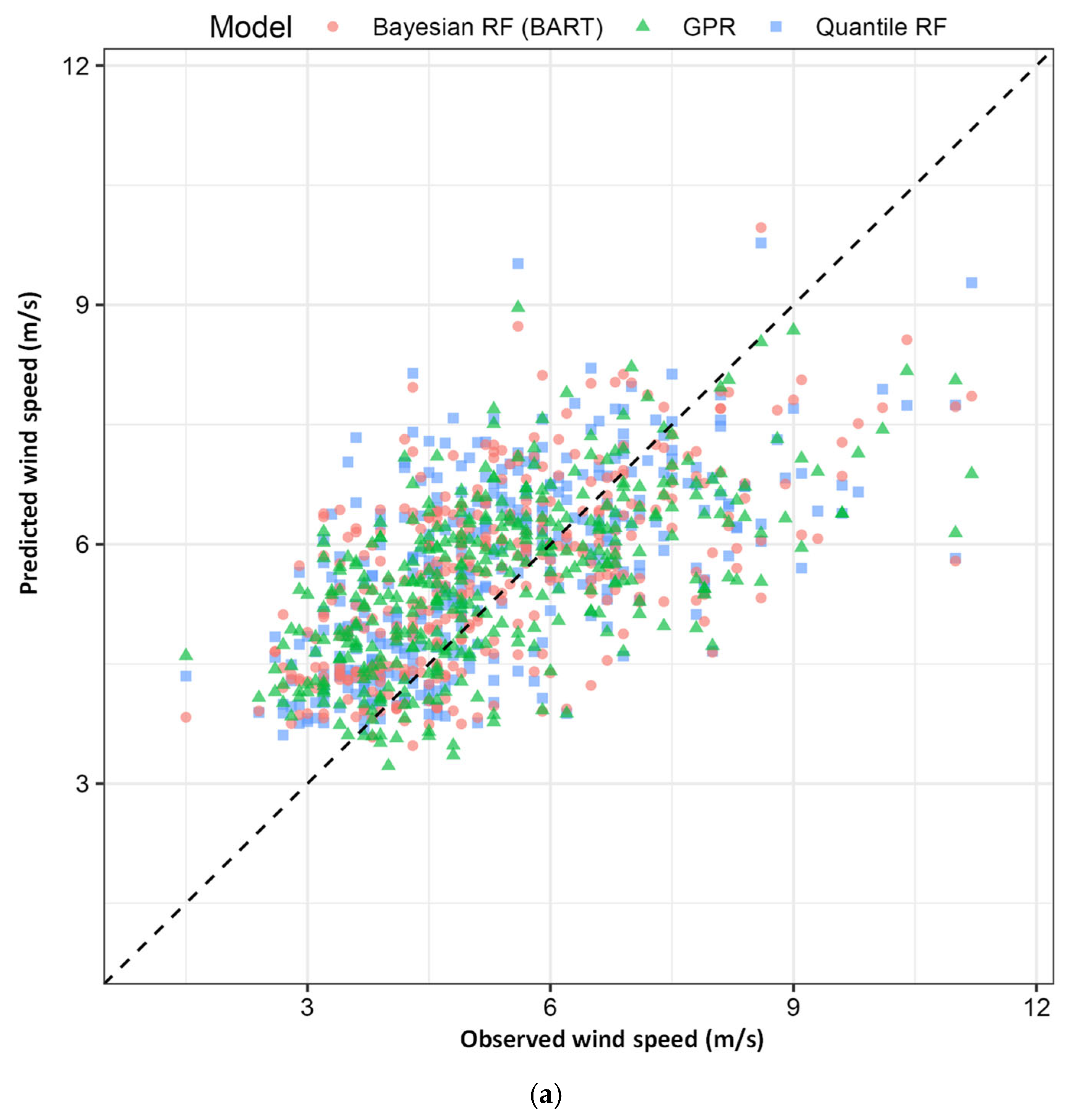
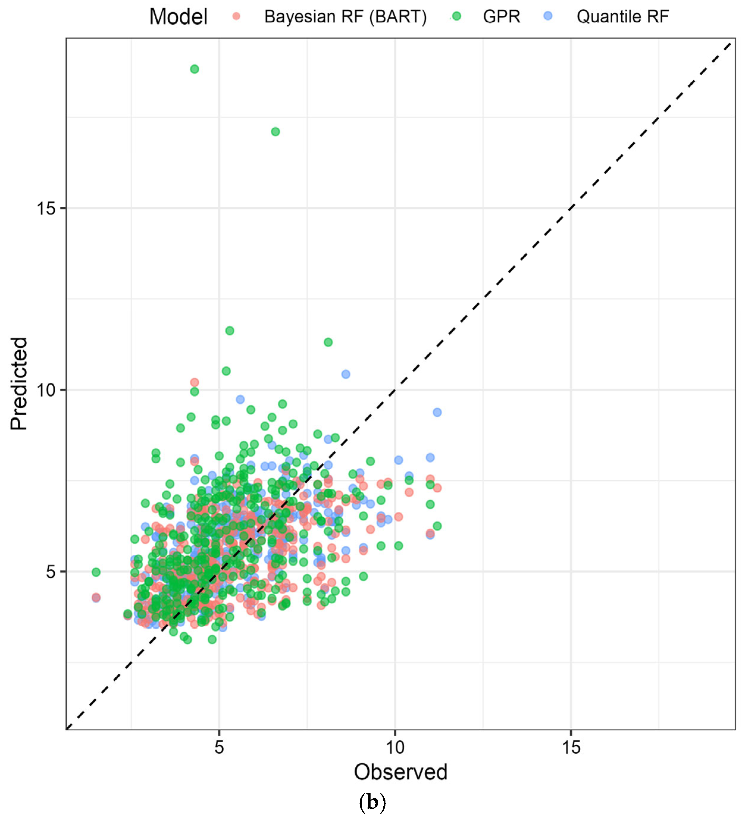
Regional pooling as seen in Figure 4 introduces substantial scatter and systematic overestimation bias, particularly at moderate wind speeds (5–10 m/s), as the global kernel smooths over local sea-breeze dynamics not captured by inland-dominated training data. Despite accuracy loss, coverage remains near-nominal, illustrating GPR’s core strength (Table 2a,b and Table 3): inflated predictive variance compensates for reduced point accuracy to maintain calibration.

4.6. Integrated Probabilistic Skill: CRPS as Unified Metric

CRPS synthesises accuracy, calibration, and sharpness into a single strictly proper score. GPR achieves the lowest CRPS at-site (1.298 m/s) and maintains this advantage regionally (1.397 m/s), despite showing the highest RMSE penalties. This apparent paradox, worse point accuracy yet better probabilistic skill, resolves when recognising that CRPS penalises miscalibration heavily: GPR’s appropriately wide predictive intervals, capturing 94% of observations, outweigh increased RMSE, yielding superior probabilistic performance. BART posts competitive at-site CRPS (1.322 m/s) but degrades most severely under pooling, driven by simultaneous RMSE increases and coverage collapse. QRF shows modest CRPS degradation, remarkable given its severe under-coverage, explained by its strong point accuracy partially compensating for interval deficiencies.

At 94580_GCW, GPR’s CRPS improves under pooling, a rare beneficial effect where broader training samples enhance tail modelling despite increased RMSE. Conversely, BART’s CRPS explodes, the largest single-site degradation observed, confirming probabilistic forecast collapse. At low-variability station 94573_CAS, all models show better CRPS, but only GPR maintains calibration, whereas BART and QRF achieve low CRPS partly through luck (under-predicting variability happens to align with realised outcomes in this year).

One-year-ahead wind speed forecasts for high-variance station 94580_GCW with 95% prediction intervals are shown in Figure 5: (a) at-site models (QRF, BART, and GPR) and (b) regional models. Black lines show observed wind speeds. Shaded regions denote 95% prediction intervals. At-site (panel a), BART and GPR achieve near-nominal coverage (0.94, 0.97) with appropriately wide intervals capturing observed variability including extreme wind events exceeding 30 m/s; QRF intervals are narrower, yielding under-coverage. Regionally (panel b), BART and QRF intervals narrow excessively, systematically under-covering observations, while GPR intervals remain adequately wide to maintain coverage despite increased RMSE. This visualisation confirms GPR’s superior interval calibration robustness under pooling.

4.7. Operational Interpretation: Translating Forecast Metrics to Energy Grid Applications

We contextualise the magnitude of forecast differences in terms of renewable energy operations for practical syntheses:

Point Forecast Accuracy (RMSE, MAE):

An RMSE difference of 0.006 m/s (or 0.26% relative increase) may appear trivial in absolute terms; however, its operational impact depends on the site wind regime and grid-level deployment scale. For example,

-

At a coastal site with mean wind speed 10.4 m/s (94580_GCW), a 0.006 m/s RMSE increase corresponds to ~0.06% increase in forecast variance.

-

Wind power output scales nonlinearly with wind speed: P ∝ v³ (cubic power law). A 0.006 m/s under-prediction can lead to ~0.2% underestimation of power output when winds are near marginal wind speeds (6–8 m/s), and negligible impact at higher wind speeds where generation is already saturated.

-

Across a 500 MW wind farm portfolio, a 0.2% systematic bias in power forecasting translates to ~1 MW forecasting error, equivalent to ~AUD 50,000 per day in energy trading costs at typical Australian NEM pricing (~AUD 50/MWh), or scheduling constraints for grid-balancing reserves.

Probabilistic Calibration (Coverage, Interval Width):

Prediction intervals failing to achieve nominal coverage (e.g., regional QRF achieving 0.70 instead of 0.95) directly impact risk management:

-

Energy traders rely on 95% prediction intervals to set confidence bounds for forward market bids. Under-coverage (0.70) means that actual wind speeds exceed the upper bound ~30% of the time (vs. expected 5%), leading to a systematic underbidding risk: generators over-commit the available capacity and face penalties when forecasted wind fails to materialise.

-

In contrast, well-calibrated intervals (e.g., GPR at coverage = 0.941) enable traders to optimise reserve margins and reduce over-procured balancing reserves, lowering system costs by ~2–5% in high-renewable-penetration grids.

Probabilistic Skill (CRPS):

CRPS differences (e.g., 0.1 m/s between models) quantify the magnitude of typical forecast errors in units of wind speed:

-

A CRPS = 1.3 m/s means that the model’s forecast distribution is, on average, displaced 1.3 m/s from the observed wind speed (combining both bias and spread).

-

For a coastal hub-height site (mean wind ~10 m/s), CRPS = 1.3 m/s corresponds to ~13% of mean climatological wind—a benchmark for “useful” probabilistic forecasting.

-

Reductions in CRPS (e.g., 0.1 m/s) translate to ~7–8% narrower forecast uncertainty, enabling tighter reserve scheduling and reduced backup generation costs.

Summary Interpretation:

While point forecast RMSE differences (0.006–0.181 m/s) appear small in absolute terms, their operational significance becomes clear when viewed through energy trading, grid balancing, and reserve-cost lenses. Regional QRF excels in point accuracy but fails in probabilistic calibration, making it suitable for energy yield estimation but unreliable for risk-sensitive operational decision-making. Conversely, regional GPR sacrifices slight accuracy for robust probabilistic calibration, making it preferable for grid reserves, wind farm dispatch, and financial hedging where interval reliability is paramount. This trade-off is central to the study’s operational recommendations (Section 5.3).

4.8. Variable Importance: Persistent Drivers and Spatial Predictor Roles

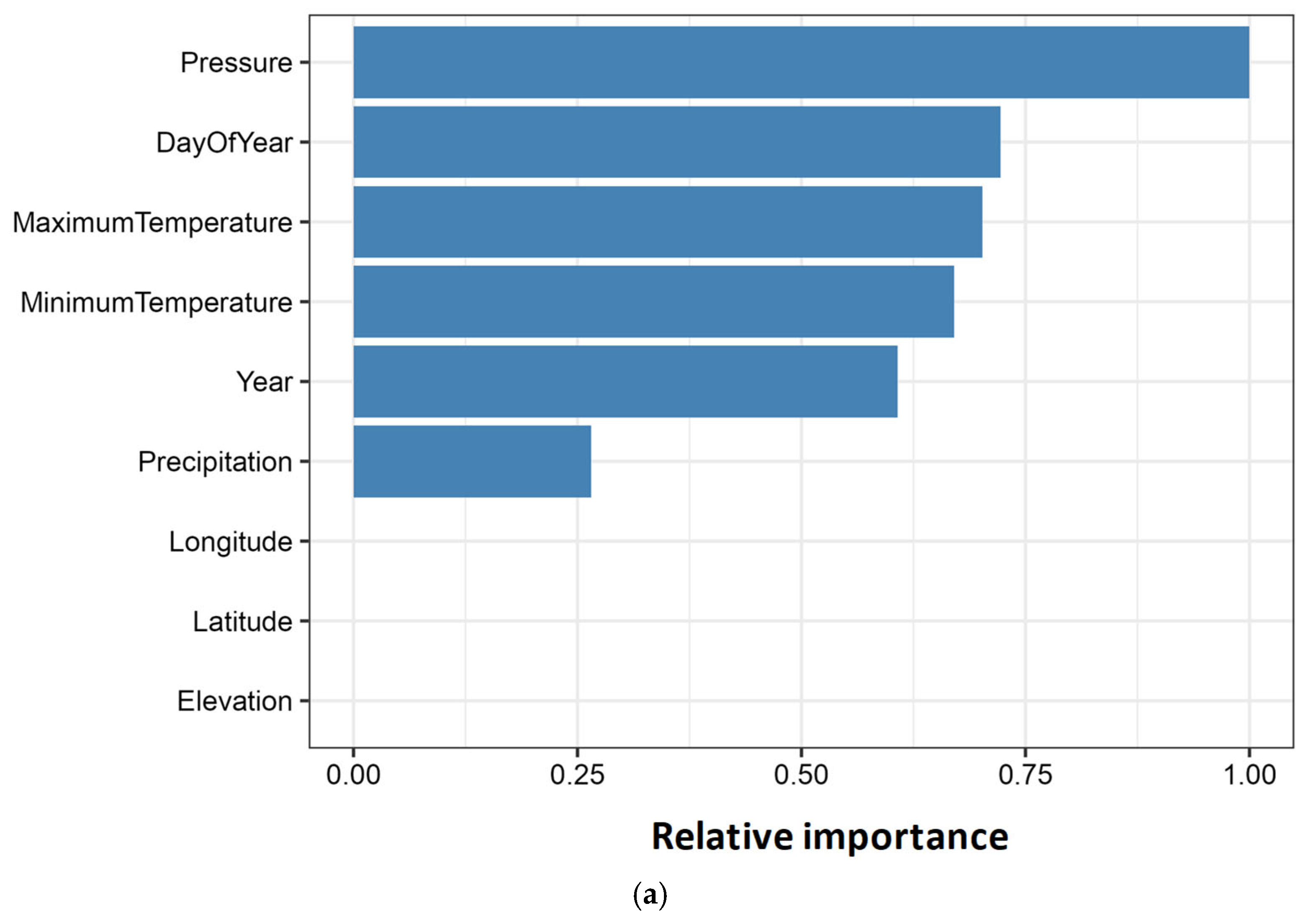
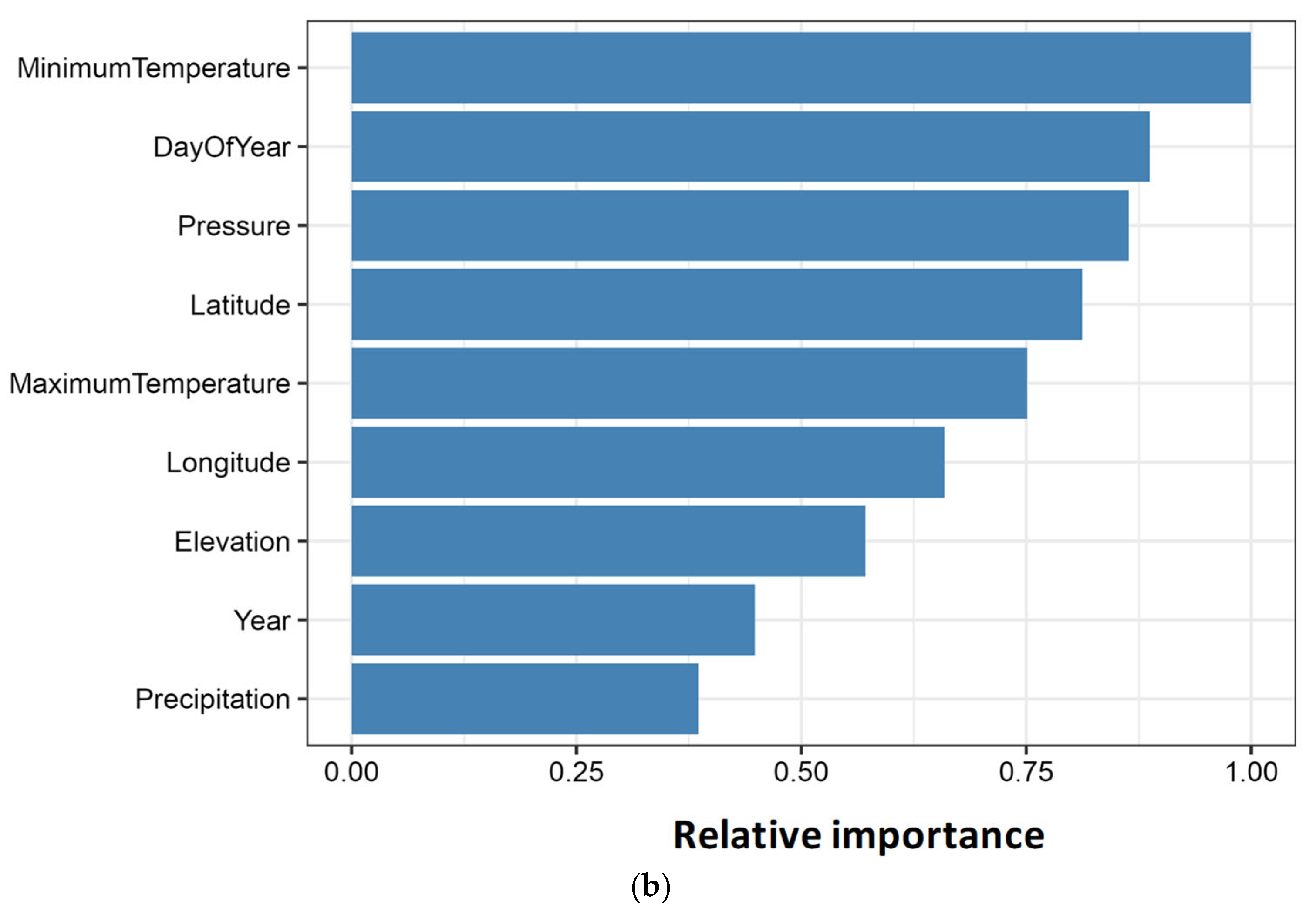
Variable importance analysis confirms that surface pressure and minimum temperature constitute the primary drivers of daily wind speed variability across all algorithms, regimes, and sites, validating the established meteorological theory linking synoptic-scale pressure gradients to near-surface wind generation and nocturnal thermal stability to boundary-layer turbulence modulation. Surface pressure directly encodes geostrophic forcing from migrating high- and low-pressure systems, while minimum temperature captures the radiative cooling effects that govern stable nocturnal boundary layer formation, suppressing or enhancing wind speeds depending on local topographic channelling and thermal advection patterns. Variable importance scores for QRF at station 94752_BAD are shown in Figure 6: (a) at-site model and (b) regional model. Importance scores are normalised permutation-based CRPS increases that are scaled. Surface pressure consistently ranks highest (importance ≈ 1.0), followed by day of year (0.7–0.75) and minimum temperature (≈ 0.70). In the regional framework (panel b), spatial predictors (latitude, longitude, and elevation) gain notable importance (0.8, 0.58, and 0.55, respectively), enabling the pooled model to differentiate coastal versus inland wind regimes. Precipitation and year remain of lower importance (< 0.40) across both regimes, particularly for precipitation, validating their exclusion from streamlined operational models.

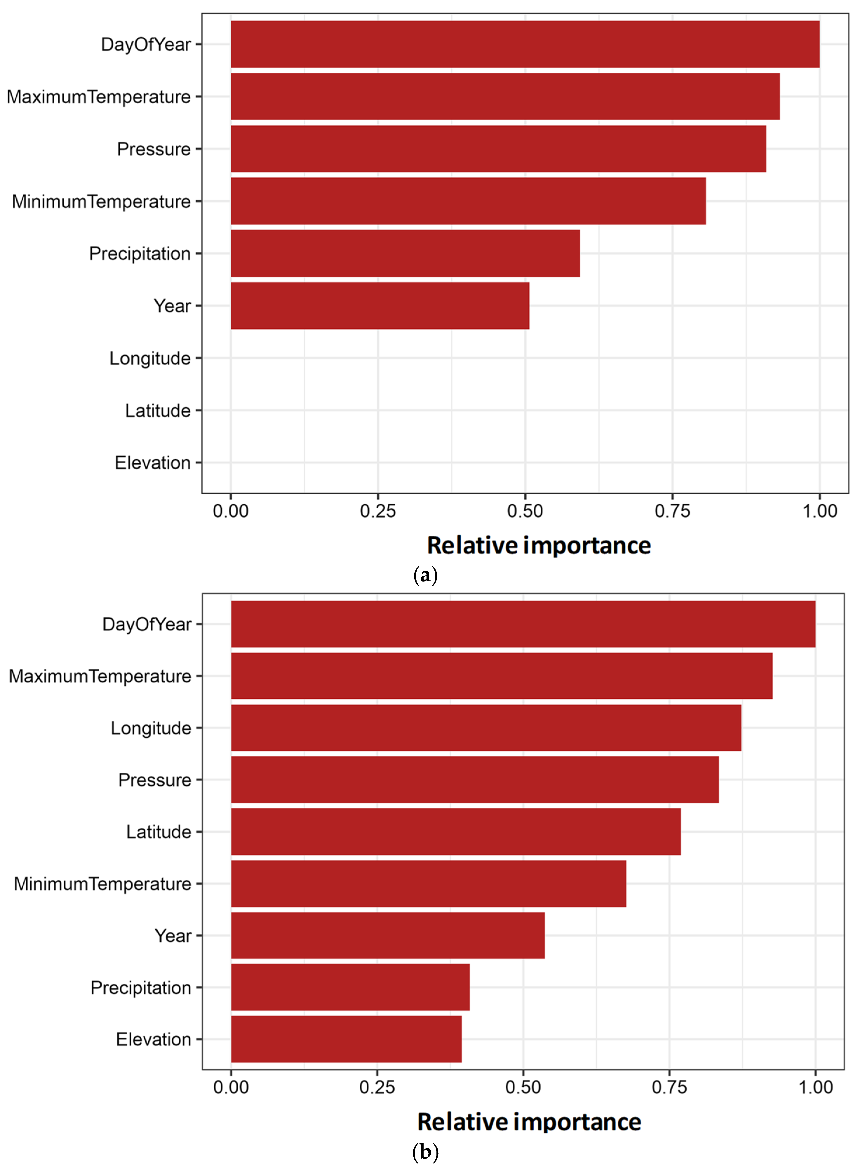
The variable importance scores for BART at station 94729_BAT, (a) at-site model and (b) regional model, are shown in Figure 7. Importance is derived from normalised posterior tree-split frequencies across MCMC samples. Pressure and minimum temperature dominate (0.8–1.0), consistent with QRF patterns. The day of year exhibits relatively high importance (≈0.75) capturing seasonal cycles. Regional BART (panel b) elevates spatial predictor’s latitude, longitude, and elevation to 0.75–0.8, ≈0.45, and 0.57 importance, respectively, crucial for the pooled model’s ability to assign station-specific wind climatologies. Precipitation shows nominal contribution (≈0.25), suggesting limited marginal predictive power for daily wind forecasts.

Overall, these variable importance patterns are consistent across all eleven stations and across QRF, BART, and GPR. Surface pressure and minimum temperature together account for approximately 60–80% of total importance, day of year contributes a robust seasonal signal (20–25%), and spatial covariates (latitude, longitude, elevation) are negligible in at-site models but rise to moderate or high importance (≈45–60% of maximum) in regional frameworks. In this sense, Figure 6 and Figure 7 provide a compact visual summary of variable importance across models and sites, highlighting a stable hierarchy of predictors that underpins the main conclusions of this study. Taken together, the variable importance profiles in Figure 6 and Figure 7 act as a summary map of predictor influence across all methods and sites: pressure and minimum temperature dominate, day of year provides a secondary seasonal signal, and spatial covariates become essential only in regional frameworks, where they encode microclimate differentiation.

This enables the algorithms to learn seasonal cycles in wind climatology driven by the annual migration of the subtropical ridge, mid-latitude storm tracks, and monsoonal influences. In regional models (Figure 6b and Figure 7b), spatial predictors—latitude, longitude—gain substantial importance (45–60% of maximum), as they provide the sole mechanism for algorithms to differentiate among geographically dispersed stations with contrasting microclimates when training on pooled data. Latitude encodes meridional gradients, longitude captures continental versus maritime exposure along the east coast, and elevation signals orographic wind enhancement and down slope wind potential.

Conversely, at-site models (Figure 6a and Figure 7a) assign minimal importance to these spatial features, as the fixed station location renders them constant (zero variance), leaving temporal meteorological covariates to explain all within-site wind variability. Precipitation and calendar year consistently rank lowest across both regimes, suggesting limited marginal predictive power for daily wind speed. Precipitation’s event-driven, zero-inflated distribution likely contributes via nonlinear interactions (e.g., post-frontal clearing enabling stronger winds) not captured by the linear marginal effects, while calendar year’s low importance indicates minimal long-term trends over the 21-year study period, consistent with stationary wind climatology assumptions.

The consistency of these importance rankings across QRF’s permutation-based scores (Figure 6), BART’s MCMC split frequency counts (Figure 7), and GPR’s permutation-based CRPS degradation validates the robustness of the identified drivers and supports operational model simplification: precipitation and year may be excluded from some sites’ streamlined forecasting systems without material accuracy loss, reducing the computational burden and data acquisition costs while maintaining interpretability. The elevation of spatial predictors, particularly elevation, to moderate-to-high importance in regional frameworks confirms that geographic information sharing is essential for capturing microclimate differentiation across Australia’s diverse topographic and coastal gradients.

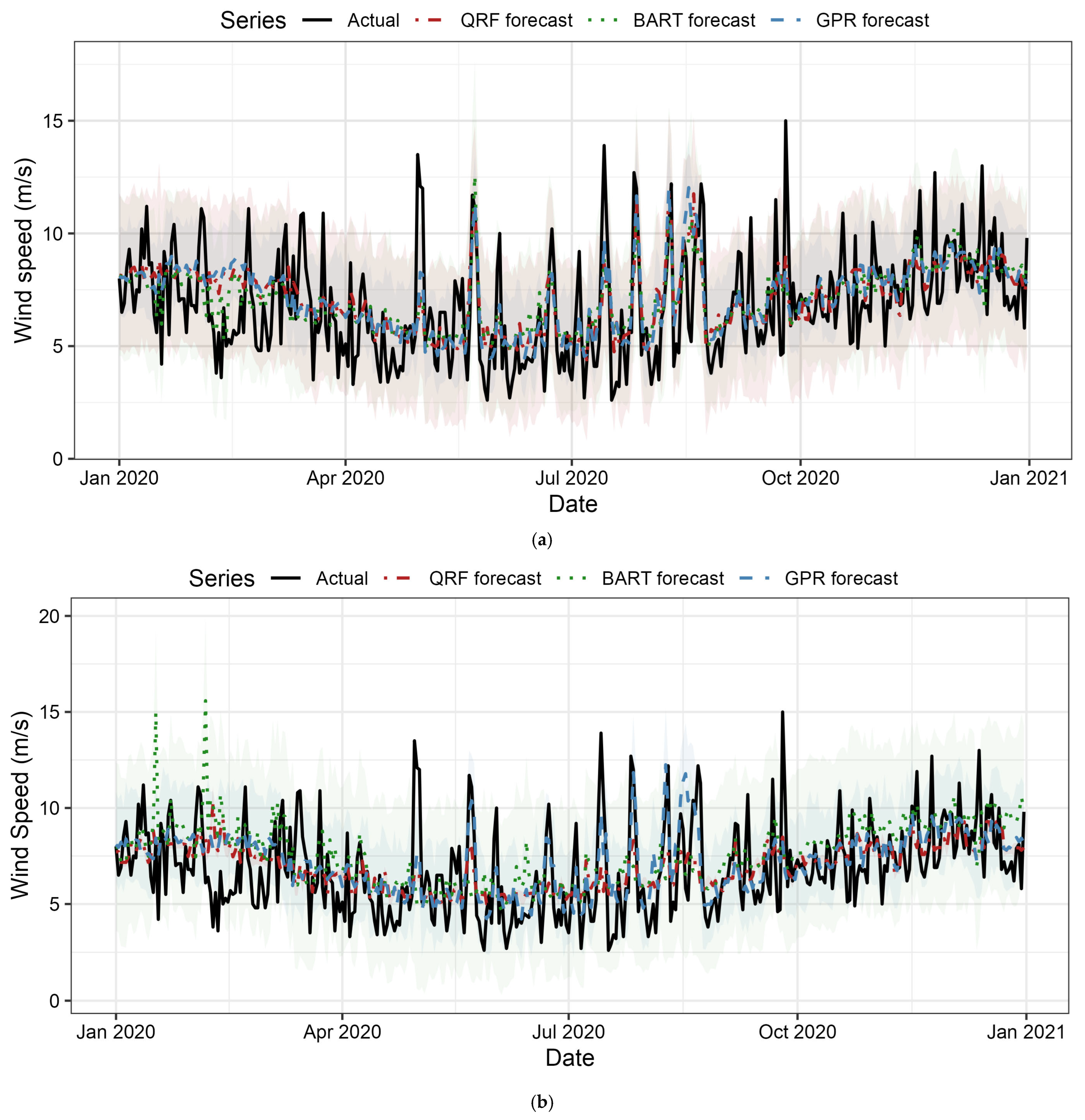
The one-year-ahead wind speed forecasts for station 94575_BRI compare all three algorithms: (a) at-site models and (b) regional models. The black solid line shows the observed wind speeds throughout 2020. The red dashed line (QRF forecast), green dotted line (BART forecast), and blue dash-dot line (GPR forecast) show the predicted medians from each algorithm. The grey, tan, and light blue shaded regions denote 95% prediction intervals for QRF, BART, and GPR, respectively. In panel (a) at-site, all three models track the observed variability with reasonable phasing, with BART and GPR intervals capturing the most extreme events (wind speeds > 12 m/s) while QRF intervals are systematically narrower, yielding under-coverage (0.67). GPR shows the widest intervals, reflecting its analytic predictive variance inflation. In panel (b) regional, QRF maintains nearly identical point forecast accuracy to at-site (RMSE 2.12 vs. 2.13 m/s), demonstrating exceptional robustness to pooling. The BART forecasts degrade moderately (RMSE increases +0.09 m/s) with visibly narrower intervals particularly in early 2020, contributing to coverage collapse (0.93 → 0.73). GPR maintains appropriately wide intervals despite larger point forecast errors (+0.36 m/s RMSE increase), preserving near-nominal coverage (0.93 → 0.92). The visual comparison confirms the quantitative findings: QRF achieves stable point accuracy but persistent under-coverage; BART calibration deteriorates under pooling; GPR sacrifices some accuracy to maintain reliable uncertainty quantification across both regimes.

4.9. Overall Synthesis

The comprehensive seven-metric evaluation reveals the fundamental algorithm trade-offs that preclude universal superiority. Optimal model selection depends on the operational context: for point forecast priority, regional QRF achieves the lowest RMSE (2.321 m/s) at 10/11 sites with negligible pooling penalty (+0.006 m/s), maintaining a reasonably high correlation (0.530) and stable MAE. However, severe under-coverage (0.70) renders its intervals operationally unreliable without post hoc recalibration via conformal prediction.

For probabilistic reliability, regional GPR is mandatory. Despite the highest RMSE penalty (+0.181 m/s), it maintains near-nominal coverage (0.941) and achieves the lowest CRPS (1.397 m/s), balancing accuracy and calibration. GPR’s kernel-based analytic variance automatically inflates under heterogeneity, preserving the uncertainty quantification essential for cost-sensitive grid operations. Figure 8 confirms that GPR’s appropriately wide intervals capture extreme events across regimes. In such settings, a method like GPR that yields lower CRPS and near-nominal coverage is operationally preferable to alternatives with slightly lower RMSE but systematically miscalibrated intervals, because it provides more reliable information about tail risks and required reserves. In terms of computational burden, GPR incurred substantially higher wall clock time and memory usage than QRF and BART for this dataset, reflecting the cost of kernel matrix operations, so its superior probabilistic calibration must be weighed against this overhead in real-time or very large-scale applications.

At-site BART offers balanced performance (CRPS = 1.322 m/s, coverage = 0.946, RMSE = 2.359 m/s) when site-specific data suffice, but regional BART is unsuitable: coverage collapses to 0.685 (−0.261), yielding miscalibrated intervals that systematically underestimate uncertainty at heterogeneous locations. Hierarchical BART extensions with site-specific random effects are needed before regional deployment.

Key mechanistic insights from variable importance are as follows (Figure 6 and Figure 7): pressure and minimum temperature drive 60–80% of forecast skill across all methods, validating physical plausibility. Spatial predictors (latitude and longitude) become critical in regional models, enabling differentiation among microclimates. Precipitation in particular contributed minimally, supporting its possible exclusion for computational efficiency. These consistent rankings across permutation-based (QRF, GPR) and split frequency (BART) metrics validate robustness. Diagnostic visualisation integration (Figure 4, Figure 5 and Figure 8): Observed-versus-predicted scatter (Figure 4) and time series trajectories (Figure 5 and Figure 8) confirm the RMSE–coverage trade-off and GPR’s wider scatter accompanies appropriately broad intervals, while QRF/BART’s tighter predictions mask dangerous under-coverage. The multi-algorithm comparison in Figure 8 directly visualises how regional pooling preserves QRF accuracy, degrades BART calibration, and yet maintains GPR reliability, validating the quantitative findings with transparent visual evidence.

5. Conclusions

5.1. Summary of Findings

This study compared three probabilistic machine learning methods—Quantile Random Forests (QRF), Bayesian Additive Regression Trees (BART), and Gaussian Process Regression (GPR)—for daily wind speed forecasting under at-site and regional frameworks using 21 years of data from eleven stations in eastern Australia. Regional QRF delivered the most stable point forecasts, with only a minimal RMSE increase under pooling, but exhibited substantial under-coverage, indicating unreliable prediction intervals in the regional model. BART achieved near-nominal coverage at individual sites yet suffered a marked collapse in calibration when pooled regionally, reflecting difficulties in representing spatially varying noise with fixed priors.

Regional GPR accepted the largest RMSE penalties but achieved the lowest CRPS (and near-nominal coverage), demonstrating robust probabilistic skill through kernel-based variance inflation across heterogeneous locations. Variable importance consistently highlighted surface pressure and minimum temperature as dominant predictors, together contributing roughly 60–80% of total influence, while spatial covariates (latitude, longitude, elevation) became important in regional models where they encode coastal–inland and orographic contrasts. The day of year provided a modest but persistent seasonal signal, whereas precipitation and calendar year had little marginal predictive value for daily wind speed.

5.2. Interpretation and Implications

These results reveal a clear trade-off between point accuracy and probabilistic calibration. QRF’s tree ensemble architecture is highly effective at capturing the timing and mean level of winds under regional pooling but tends to generate overly narrow tails, producing intervals that understate risk for grid and market operations. BART’s behaviour underscores the sensitivity of Bayesian tree models to prior specification. Priors calibrated to at-site variability do not automatically generalise to heterogeneous regional data, leading to under-dispersed uncertainty estimates when pooling is aggressive.

GPR occupies the opposite corner of this trade-off, delivering slightly less accurate point forecasts while maintaining well-calibrated prediction intervals in regional settings. For deterministic tasks such as multi-week energy yield estimation, regional QRF is therefore attractive. For reserve sizing, risk management, and reliability assessment, regional GPR is preferable because systematic under-coverage can be more damaging than modest RMSE differences. The stability of the predictor hierarchy across all methods suggests that operational systems should prioritise high-quality pressure and temperature information and the careful representation of spatial gradients. Weak predictors such as calendar year can routinely be omitted when data or computational budgets are constrained.

5.3. Limitations and Future Research

The analysis is restricted to daily averages and to eleven stations in New South Wales and Queensland, so extensions to sub-daily horizons, additional regions, and more complex terrain are needed to fully generalise the method rankings. The predictor set was deliberately parsimonious; incorporating additional physically motivated features (e.g., shear, stability indices, NWP-derived flow metrics) may further improve performance but raises questions about dimensionality, interpretability, and robustness.

Future research should explore hierarchical or multi-level Bayesian formulations that allow BART- or GPR-type models to pool information while preserving site-level calibration. It should also investigate ensemble or stacking schemes that dynamically weight QRF, BART, and GPR by regime, season, or lead time. Adaptive recalibration frameworks and integration with climate projection ensembles offer promising routes to link short-term probabilistic forecasts with long-term planning for high-renewables power systems. Quantitatively, however, the reported skill scores and method rankings are conditioned on the NSW–QLD climate and station network, so extrapolation to other regions should be made cautiously even though the modelling framework itself is directly transferable.