Intensification of SUHI During Extreme Heat Events: An Eight-Year Summer Analysis for Lecce (2018–2025)

Abstract

The effects of extreme heat events on Surface Urban Heat Island Intensity (SUHII) were investigated in Lecce (southern Italy) during the summer months (June–August) from 2018 to 2025. The analysis began with the identification of heatwave frequency, duration, and intensity using the Warm Spell Duration Index (WSDI), based on a homogenized long-term temperature record, which indicated a progressive increase in persistent extreme events in recent years. High-resolution ECOSTRESS land surface temperature (LST) data were then processed and combined with CORINE Land Cover (CLC) information to examine the thermal response of different urban fabrics, compact residential areas, continuous/discontinuous urban fabric, and industrial–commercial zones. SUHII was derived from each ECOSTRESS acquisition and evaluated across multiple diurnal intervals to assess temporal variability under both normal and WSDI conditions. The results show a consistent diurnal asymmetry: daytime SUHII becomes more negative during WSDI periods, reflecting enhanced rural warming under dry and highly irradiated conditions, despite overall higher absolute LST during heatwaves, whereas nighttime SUHII intensifies, particularly in dense urban areas where higher thermal inertia promotes persistent heat retention. Statistical analyses confirm significant differences between normal and extreme conditions across all classes and time intervals. These findings demonstrate that extreme heat events alter the urban–rural thermal contrast by amplifying nighttime heat accumulation and reinforcing daytime negative SUHII values. The integration of WSDI-derived heatwave characterization with multi-year ECOSTRESS observations highlights the increasing thermal vulnerability of compact urban environments under intensifying summer extremes.

1. Introduction

Urban planning and sustainable development are essential for enhancing the resilience and well-being of cities increasingly exposed to the combined pressures of climate change and rapid urbanization. Understanding how climatic factors interact with the urban microclimate is fundamental to improving air quality, mitigating thermal discomfort, and promoting effective climate adaptation strategies [1].

One of the most challenging aspects of contemporary urban climate research is mitigating the microclimatic effects of urbanization, among which the Urban Heat Island (UHI) phenomenon plays a central role. The UHI refers to the increase in air temperature within urban areas compared to surrounding rural environments, resulting from the combined influence of surface properties, land-use patterns and urban morphology. The magnitude of this temperature difference, referred to as UHI Intensity (UHII), can reach several Celsius degrees on annual averages and up to 12 °C under calm and clear nocturnal conditions. Moreover, extreme heat events such as heatwaves are known to exacerbate UHII, such as higher background temperatures, reduced nighttime cooling, and increasingly dry surface conditions, amplifying the thermal contrast between urban and rural areas [2,3].

Several physical mechanisms contribute to the formation of UHI: the modification of surface albedo and thermal capacity by construction materials, which enhances heat storage; the reduction in evapotranspiration due to impervious surfaces, which decreases latent heat fluxes; and the geometry of urban canyons, which increases multiple reflections and restricts radiative loss. In addition, increased surface roughness associated with buildings alters wind flow, affecting both heat dispersion and pollutant transport [4]. Recent reviews, such as Rajagopal et al. [5], provide a comprehensive synthesis of how environmental and planning interventions can influence UHI magnitude.

Land cover information provides a crucial foundation for these analyses, as it allows for the systematic classification of urban and non-urban surfaces according to their physical and environmental characteristics. Beyond climate assessment, land cover mapping supports sustainable urban development by identifying opportunities for green infrastructure such as urban forests, green roofs, and permeable surfaces, which help mitigate the Urban Heat Island (UHI) effect, enhance biodiversity, and promote public health [6]. In this framework, the standardized and comparable structure of the CORINE Land Cover (CLC) database offers a valuable tool for assessing how surface characteristics influence local climate conditions across Europe.

The CLC database classifies land cover into categories describing artificial surfaces, agricultural land, wooded and semi-natural areas, and other relevant types [7,8]. Its spatial consistency and continental coverage make it an essential reference for urban planners and climate researchers studying the influence of land cover on environmental and climatic processes.

Urban thermal environments are typically investigated through air temperature data, satellite-derived land surface temperature (LST) products [9,10,11,12], and numerical models. Among these approaches, satellite LST has proven particularly effective for analyzing the Surface Urban Heat Island (SUHI) effect, providing spatially continuous and globally consistent observations of surface temperature distributions [13,14]. However, current thermal datasets have inherent limitations: low-resolution instruments such as MODIS and Sentinel-3 provide high temporal frequency but limited spatial detail (~1 km²), whereas high-resolution missions such as Landsat or ASTER offer finer spatial information but reduced temporal coverage and limited nighttime observations [15,16,17,18,19].

To overcome these constraints, this study employs the Ecosystem Spaceborne Thermal Radiometer Experiment on Space Station (ECOSTRESS), which provides high-resolution (70 m × 70 m) thermal observations at variable times throughout the day. Installed on the International Space Station in 2018, ECOSTRESS enables an unprecedented characterization of diurnal and intra-urban temperature variability [20]. Its usefulness for urban climate studies has been demonstrated in several recent works [20,21,22,23,24,25], though most analyses have focused on short time spans, underscoring the need for long-term, multi-year datasets. Recent global assessments, such as the analysis of SUHI intensity in 1031 cities conducted by Yao et al. [26], have highlighted the considerable variability in thermal contrasts between urban and rural areas determined by regional climate and land cover composition using MODIS and Landsat data.

Despite the increasing use of satellite thermal data, relatively few studies have explicitly examined how LST or SUHI intensity varies across CLC land cover classes. Stathopoulou et al. [27] combined Landsat ETM+ data with CLC information to assess the daytime UHI effect in major Greek cities, showing the key role of land cover in shaping thermal anomalies. Stamou et al. [28] investigated similar correlations in Thessaloniki using Landsat imagery and vegetation indices, identifying a general warming trend. García [29] analyzed combined Landsat 8 and Sentinel-3 data for 2019 but limited the temporal scope to one year. Albini et al. [30] and Hellings and Rienow [31] used Landsat and MODIS data, respectively, revealing temperature contrasts of 4.0–6.0 °C between impervious and vegetated surfaces. Renc et al. [32] confirmed statistically significant differences in LST among urban, industrial, agricultural, and forest classes, while Sfîcă et al. [33] demonstrated how land use changes based on CLC data between 2000 and 2018 intensified the UHI effect in Romania. Similarly, Naeem and Mahmood [34] reported that agricultural lands consistently exhibited the lowest LST values in Multan, emphasizing their potential role in mitigating urban heat under conditions of rapid land-use transformation.

High-resolution ECOSTRESS observations make it possible to overcome many of the limitations of previous datasets, allowing the continuous monitoring of diurnal and intra-urban temperature variations. Furthermore, while the use of absolute LST values provides direct information about thermal exposure, the SUHI effect represents a normalized metric that enables comparison between urban and rural conditions under different climatic regimes. This normalization is particularly important when analyzing the impact of extreme events, since it allows the quantification of how the urban–rural thermal contrast evolves under both normal and heatwave conditions, albeit it cannot be considered a unique proxy for assessing heat stress [35].

In this study, absolute LST is first analyzed as a measure of urban heat exposure, followed by an evaluation of SUHI intensity in relation to CLC land cover classes in Lecce, a medium-sized city in southern Italy. The analysis focuses on the summer months of June, July, and August and examines SUHI variability during extreme heat events, identified through the WSDI, compared with non-extreme conditions to assess spatial and temporal differences in urban thermal behavior.

This work addresses the main limitations of previous studies, often constrained by short time frames or low spatial resolution, by analyzing a multi-year ECOSTRESS dataset (2018–2025) integrated with CLC-based land cover data. Unlike earlier studies on Lecce such as Donateo et al. [36], which investigated the UHI effect using in situ measurements, Esposito et al. [15], which analyzed SUHI Intensity using Sentinel-3 data limited to specific hours of the day, and Pappaccogli et al. [25], which examined diurnal LST variability between 2018 and 2024, this research extends the temporal coverage to 2025, captures the full diurnal cycle, and focuses specifically on SUHI dynamics under both normal and extreme heat conditions within the CLC classification framework.

The results contribute to a deeper understanding of how urban geometry and land-use influence thermal behavior and demonstrate the relevance of SUHI analysis as a normalized indicator for comparing the impacts of extreme heat events. This approach underscores the importance of combining high-resolution thermal data with standardized land cover classifications to support climate-sensitive urban planning and sustainable adaptation strategies [37].

2. Materials and Methods

2.1. Study Areas

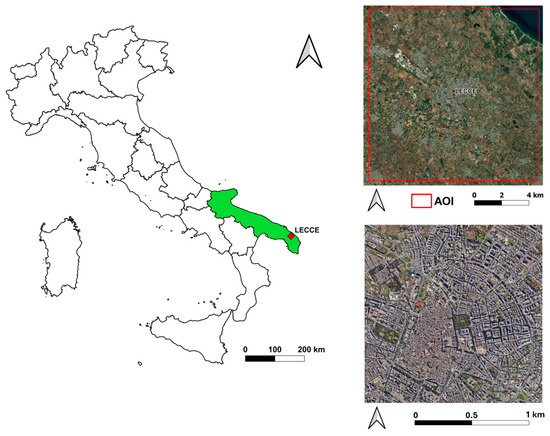
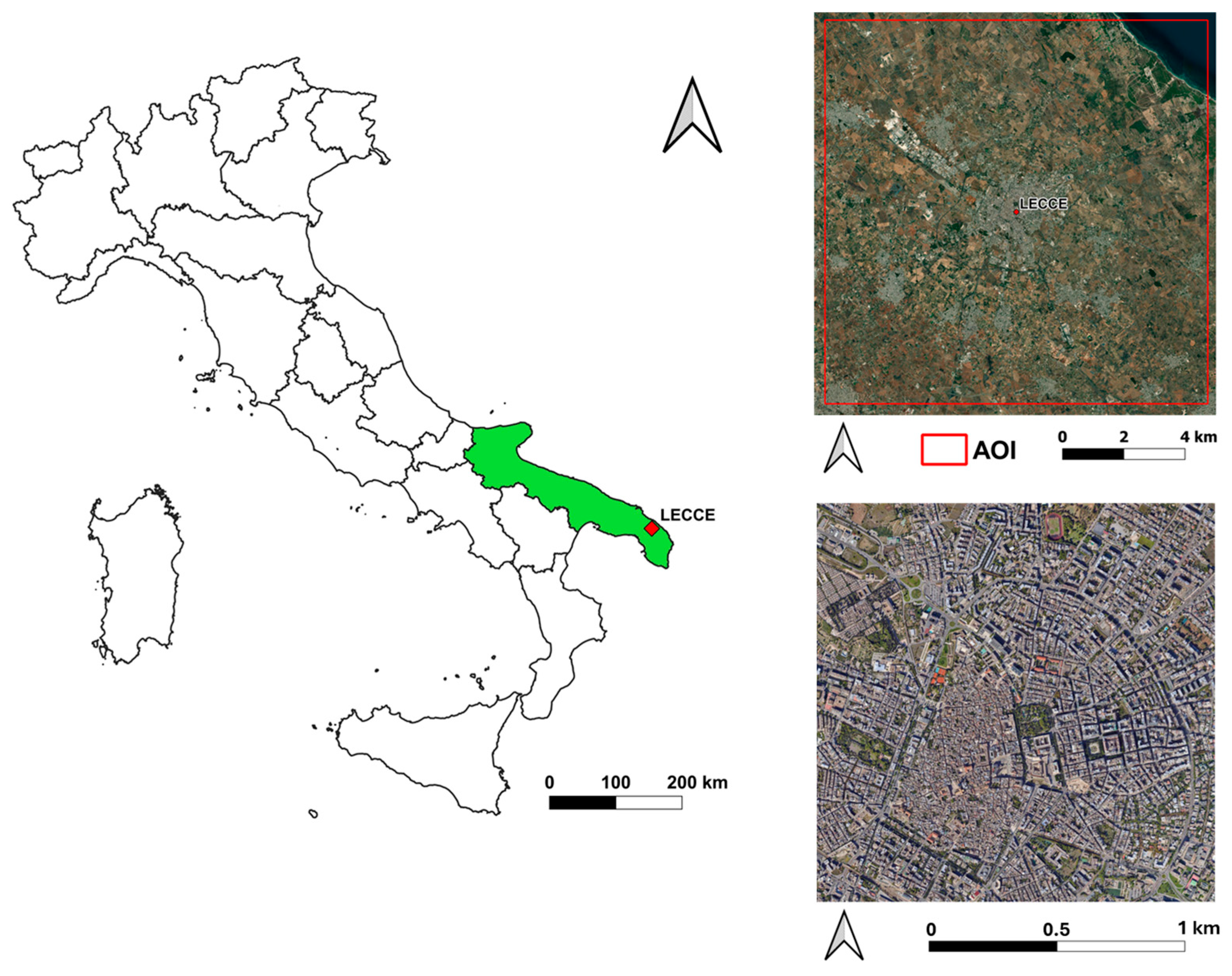
This study focuses on the city of Lecce, a medium–sized urban area with approximately 95,000 inhabitants according to ISTAT [38], located in southeastern Italy (40°21′7.24″ N, 18°10′8.9″ E, see Figure 1). Since the 2000s population has remained relatively stable, without a significative urban expansion and land use change. The city stands on flat land about 40–50 m above sea level, about 13 km from the Adriatic Sea and 25 km from the Ionian coast. Lecce has a radial urban structure that expands northwest towards the industrial districts, east towards the coast, and south towards the residential neighborhoods. The historic center is characterized by narrow streets and closely spaced buildings of various orientations, while the more recent neighborhoods have a more regular urban layout [39]. Lecce has a typical Mediterranean climate (Csa according to the Köppen–Geiger classification), with hot, dry summers and mild, humid winters (Köppen–Geiger climate classification world map, accessed on 3 October 2025). During the summer, the Salento peninsula is often subject to intense heatwaves caused by persistent subtropical high–pressure systems [40]. Mean annual rainfall is around 650 mm [41] concentrated in winter and autumn, while summer rainfall is scarce and mainly convective [42]. The mean annual temperature is around 16.0–17.0 °C, with minimal spatial variations between the east and west coasts. Wind patterns are dominated by northwesterly and southwesterly currents, which determine local ventilation and the spatial distribution of surface heat [41].

Figure 1. (left) Location of the city of Lecce within the Apulia region (highlighted in green), south–east Italy; (top-right) red square represents the area of interest (AOI); (bottom-right) zoomed in AOI representing the urban area of Lecce (40°21′7.24″ N, 18°10′8.9″ E).

2.2. Land Cover Analysis Based on CLC

To enable a comparison between intra–urban variability and dominant land cover characteristics, this study adopts the CLC classification system. The CLC program was launched in the late 1980s as part of the Coordination of Environmental Information initiative to standardize the collection of land cover data across Europe and support the formulation of environmental policies. Since then, it has become the main spatial reference dataset for land cover mapping within the European Economic Area.

The CLC database is produced by the Copernicus Land Monitoring Service, a component of the European Union’s Copernicus Earth observation program. It is derived from high–resolution satellite imagery provided through the EuroDataCube platform (https://collections.eurodatacube.com/, accessed on 10 October 2025). The inventory comprises 44 land cover and land use classes, which describe the physical and biophysical characteristics of surfaces across Europe (https://land.copernicus.eu/content/corine-land-cover-nomenclature-guidelines/html/, accessed on 1 December 2025). The standard CLC product has a spatial resolution of 100 m and it is updated on a six-year cycle (1990, 2000, 2006, 2012, 2018, and 2024 but not yet available), providing consistent long-term land cover information across Europe. In this study, these data were combined with the higher-resolution CLC+ Backbone 2023 product (10 m × 10 m) to refine the definition of rural areas.

For this analysis, three urban CLC classes representative of built environments were selected:

• CLC 1 (1.1.1—Continuous urban fabric): areas dominated by buildings and transport networks, where impervious materials (e.g., asphalt, concrete) cover more than 80% of the surface. Vegetation and bare soil are scarce.
• CLC 2 (1.1.2—Discontinuous urban fabric): mixed areas containing both artificial and natural elements, where impervious surfaces occupy 30–80% of the land surface.
• CLC 3 (1.2.1—Industrial or commercial units): areas used primarily for industrial, commercial, or public service purposes, characterized by compacted or sealed surfaces with sparse vegetation, typically in the form of lawns or ornamental areas.

A rural reference class (CLC rur) was defined using the CLC+ Backbone 2023 dataset (10 m × 10 m resolution). This class includes all CLC categories 2–9, representing agricultural, forest, semi-natural, and other non-urban land covers. The study area does not include rivers, lakes or other permanent water bodies.

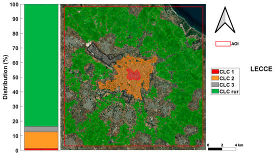
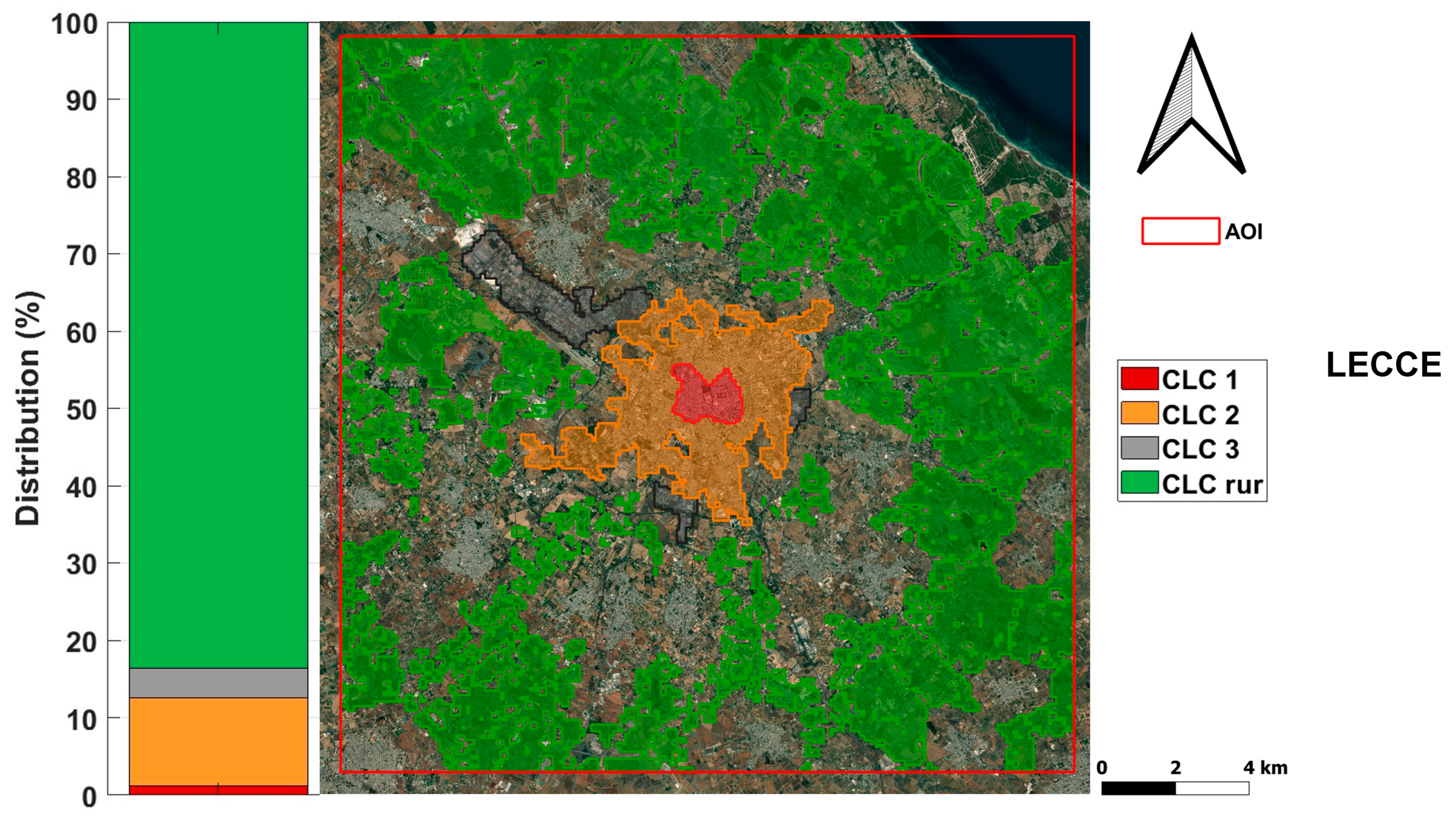
To prevent thermal contamination from nearby built-up areas, two buffering steps were applied: a 500 m buffer around all urban classes (CLC 1, 2, and 3) was removed from the rural mask, followed by the exclusion of a 100 m buffer derived from sealed artificial surfaces (CLC class 1) in the CLC+ Backbone 2023 layer. These operations ensured that rural LST values were not affected by adjacent impervious or urbanized surfaces. Finally, the three CLCs and the rural class were merged into a single harmonized dataset for subsequent SUHI and LST analyses. The percentage distribution of CLC classes and the spatial distribution map are presented in Figure 2.

Figure 2. Percentage and spatial distribution of CLC classes for the city of Lecce.

2.3. Collecting ECOSTRESS Data

The LST data used in this study were obtained from the ECOSTRESS Level–2 Land Surface Temperature and Emissivity (ECO2LSTE) product, distributed by the NASA Land Processes Distributed Active Archive Center (LP DAAC) (https://lpdaac.usgs.gov/, accessed on 16 September 2025). The ECOSTRESS mission, managed by NASA’s Jet Propulsion Laboratory, provides multi–level thermal datasets, among which the Level 2 LSTE product was selected for its combination of high spatial resolution and validated accuracy.

The ECOSTRESS LST product is derived using the Temperature Emissivity Separation (TES) algorithm, a physics–based approach that estimates surface temperature and emissivity from five infrared thermal bands covering 8–12.5 µm [43]. The final product has a spatial resolution of 70 m × 70 m, resampled from the native footprint of 38 m × 68 m, and each scene covers an area of approximately 400 km along the orbital path, allowing for regional–scale analysis.

Validation efforts have confirmed the high reliability of ECOSTRESS LST data. According to the official algorithm documentation, the expected accuracy is between 1 K across different land cover types [16]. Subsequent assessments by the ECOSTRESS scientific team reported uncertainties of less than 1 K [43], while a recent global validation found a root mean square error (RMSE) of 1.07 K, a mean absolute error (MAE) of 0.40 K, and an R² > 0.99 at multiple sites [44].

In this study, ECOSTRESS LST data were analyzed to assess summer LST variability between 2018 and 2025 and to estimate SUHII. Focusing on the summer period allows us to study the peak seasonal thermal response of urban surfaces, which is essential for understanding the spatial and temporal dynamics of heat exposure and supporting urban adaptation strategies.

All available ECOSTRESS images acquired during the summer from 2018 to 2025 were retrieved, along with their cloud mask and quality control (QC) levels. Two levels of data filtering were then applied:

• Removal of cloud proximity. To avoid contamination from unresolved or edge–affected clouds, pixels within an 8–pixel buffer (~600 m) of detected cloudy areas were excluded from each scene. This eliminated possible artifacts and shadow effects.
• Quality flag filtering. Bit–coded QC levels were used to retain only valid LST retrievals. Pixels flagged with missing or corrupted L1B data, sensor anomalies, or cloud cover were discarded, retaining only those labeled as “good quality L1B data” according to the ECOSTRESS User Guide (https://lpdaac.usgs.gov/documents/1574/ECOL2_User_Guide_V2.pdf accessed on 10 November 2025).

After the two quality checks, a third criterion was applied to ensure adequate coverage of urban areas. Only images with at least 75% of valid pixels located within the three urban CLC classes (1.1.1, 1.1.2, and 1.2.1) were retained. Images below this threshold were discarded to maintain consistent and representative urban coverage.

The initial dataset comprised 210 images acquired during the JJA period from 2018 to 2025. After all filtering steps, 129 images were retained for analysis. The annual distribution of images and summary statistics (mean, min, max, 25th and 75th percentiles, and standard deviation) for each class are shown in Table 1, which highlights the interannual variability and overall consistency of the data over the study period.

Table 1. Number of images and LST (°C) statistics per year.

	2018	2019	2020	2021	2022	2023	2024	2025
N. Images	8	15	13	21	16	19	12	25
Mean	38.5	34.2	34.1	38.8	36.8	38.0	39.0	35.4
Std	8.4	7.7	7.7	7.9	8.6	9.2	8.7	8.9
25 prt	30.3	28.1	26.2	33.7	29.8	29.6	31.6	27.1
75 prt	46.1	41.6	41.1	44.7	43.6	45.4	45.4	43.1
min	28.0	26.0	27.1	29.4	27.6	27.7	29.5	26.3
max	47.0	41.0	39.8	47.2	45.4	48.9	48.0	41.0

SUHII Calculation and WSDI Identification

SUHII is obtained as the difference between the LST of each urban pixel (CLC classes 1, 2, and 3) and the median LST value of the rural CLC classes in each image; positive values indicate a warmer urban surface while negative values indicate warmer rural surroundings indicating a positive or negative SUHII.”. Using the median ensures greater statistical robustness and reduces the influence of outliers [15].

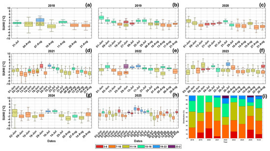
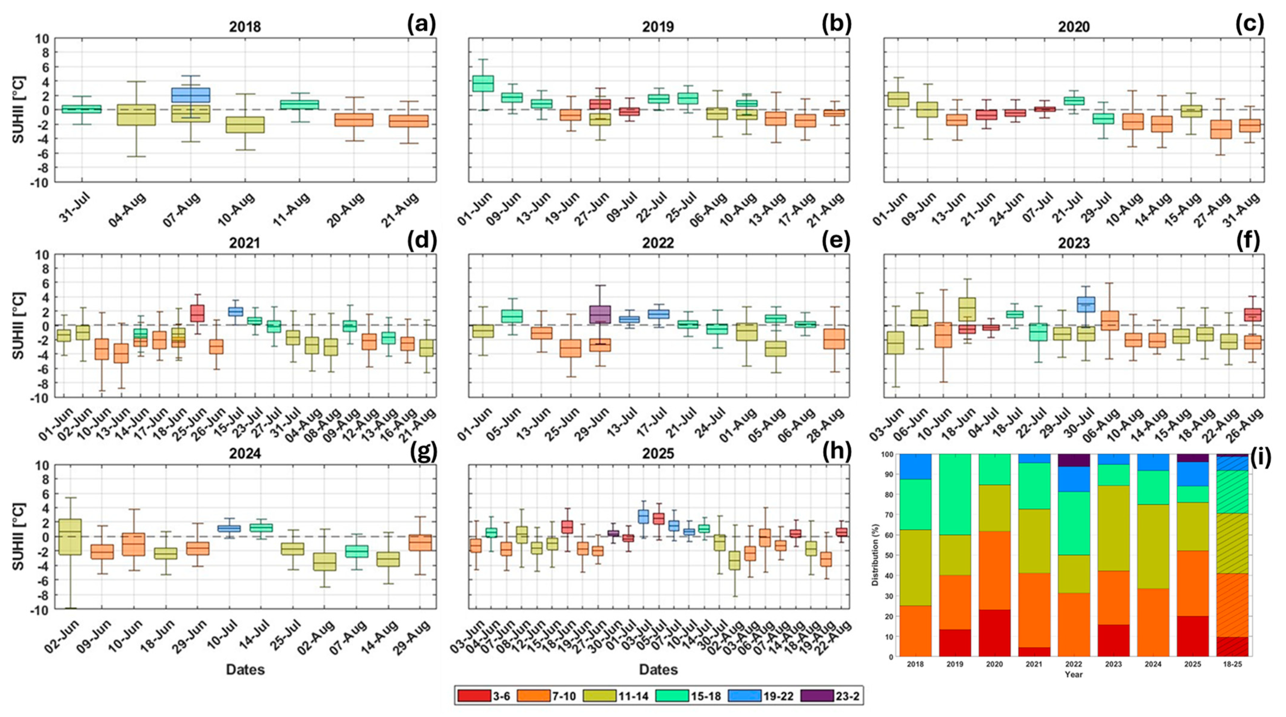
SUHII diurnal variability is obtained by dividing the dataset into six-time intervals: 03:00–06:00, 07:00–10:00, 11:00–14:00, 15:00 to 18:00, 19:00 to 22:00 and 23:00 to 02:00 (local time). This classification ensured a balanced representation of images throughout the day, providing a robust and statistically significant analysis of LST temporal patterns. The distribution of images in these intervals is shown in Figure 3 in Section 3.1.

Figure 3. Panels (a–h) show boxplots of SUHII derived from each valid ECOSTRESS image for the city of Lecce, color-coded by time slot during the summer season. Panel (i) shows the percentage of ECOSTRESS acquisitions falling within each time slot for the different years. The whiskers extend to ±2.7 standard deviations, encompassing 99.3% of the data.

Extreme heat events were identified through the WSDI index, which represents the annual count of days on which the maximum daily temperature exceeds the 90th percentile of the reference period (1961–1990), calculated using a 5-day window [45,46,47]. The reference data were collected from the conventional meteorological station located in Taviano (39°58′58.4″ N, 18°5′20.3″ E). To ensure the reliability of the daily temperature records, homogeneity tests, including Pettitt’s test, four variants of Buishand’s test, and the Standard Normal Homogeneity Test (SNHT), were performed using the pyHomogeneity Python 3.10.19 package [48]. These tests verified that the dataset was unaffected by non-climatic shifts such as changes in instrumentation, station relocation, or observational practices, confirming the homogeneity of the time series.

Following the method proposed by Fischer and Schär [49], Heatwaves (HW) were defined as a period of at least six consecutive days with a maximum temperature above the 90th percentile of the reference period. The analysis was conducted for the summer season for each year of the study period.

3. Results and Discussion

3.1. SUHII Based on ECOSTRESS Images

This analysis includes SUHII values derived from ECOSTRESS images that passed the quality tests. By considering all available images across different years and time slots, it provides a comprehensive overview of the analyses presented in this study, aimed at assessing and quantifying the limitations and advantages of using ECOSTRESS imagery.

The temporal acquisition reveals a predominance of daytime observations in the analyzed period. Most images (about 80%) were collected between 07:00 and 10:00, 11:00–14:00, and 15:00–18:00 local time, while acquisitions during the evening (19:00–22:00) and night (23:00–02:00) were less frequent or completely absent in some years.

However, despite the unbalanced distribution, the dataset provides complete coverage across different hours of the day. It is also worth noting that, although nighttime images are fewer, they depict a more homogeneous thermal environment than daytime acquisitions and may therefore be more representative of the intra-urban thermal variability. This behaviour is consistent with multi-city analyses performed by Esposito et al. [50], which show that nighttime SUHII exhibits lower spatial heterogeneity and higher statistical stability compared to daytime conditions across Italian cities, leading to more robust model performance even when nighttime acquisitions are fewer.

Furthermore, the inclusion of numerous images and the use of averaged patterns ensure that the analysis is not influenced by potential outliers or specific meteorological conditions. When examining the distribution by individual year, one or more time-slot classes are absent in all years except 2025, which exhibits a more uniform temporal coverage. This characteristic is particularly relevant for annual analyses, such as that presented in Section 3.2.

The boxplots in Figure 3 show that median SUHII values remain close to zero on most acquisition dates, indicating the predominance of weak or negative SUHI intensity during summer daytime conditions. This behavior is consistent over the years, with limited interannual variability. Positive anomalies, particularly evident in some late afternoon or evening acquisitions, rarely exceed 2.0 °C and do not show a systematic temporal trend. The color scale, which represents the time of acquisition, highlights a clear dependence of SUHII amplitude on the time of day. Observations acquired between 07:00 and 14:00 (orange and gold) generally show more negative values, reflecting stronger solar heating and lower evaporative cooling capacity of the surrounding rural areas compared to the urban center. In the late afternoon (15:00 to 18:00, cyan), SUHII values tend to increase towards zero or become slightly positive, illustrating the delayed release of heat stored by urban materials. The evening and nighttime acquisitions (19:00–22:00, blue; and 23:00–02:00, purple) show positive values, confirming the onset of the nighttime SUHI phase, during which rural areas cool more rapidly while urban surfaces release the heat accumulated during the day.

Overall, these results confirm the absence of a persistent positive SUHII in Lecce and indicate that the urban–rural thermal contrast is primarily driven by daytime radiative forcing and surface energy exchange rather than by long-term morphological or land cover changes. The city’s high-albedo materials and the low soil moisture of the surrounding rural areas contribute to this pattern, where rural surfaces often exceed urban temperatures during the day. The historic center, characterized by light-colored buildings, pavements, and narrow streets, is largely constructed from local limestone (“Pietra Leccese”) with high reflectance and distinctive thermal properties [36,51]. The combination of elevated surface albedo and limited solar exposure within the compact urban fabric, as also noted by [52,53,54,55], likely mitigates surface heating, an effect reinforced by the low soil moisture of nearby rural zones. Consequently, the negative SUHII values observed in Lecce align with the previously documented local air heat island inversion in the city center, where slightly lower air temperatures occur during early summer hours [36]. Building on this diurnal characterization, the next section examines how SUHII varies across different years, to assess whether interannual changes in meteorological conditions or acquisition timing systematically influence the observed urban–rural thermal contrast.

3.2. Annual Summer Variability of SUHII

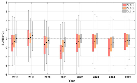
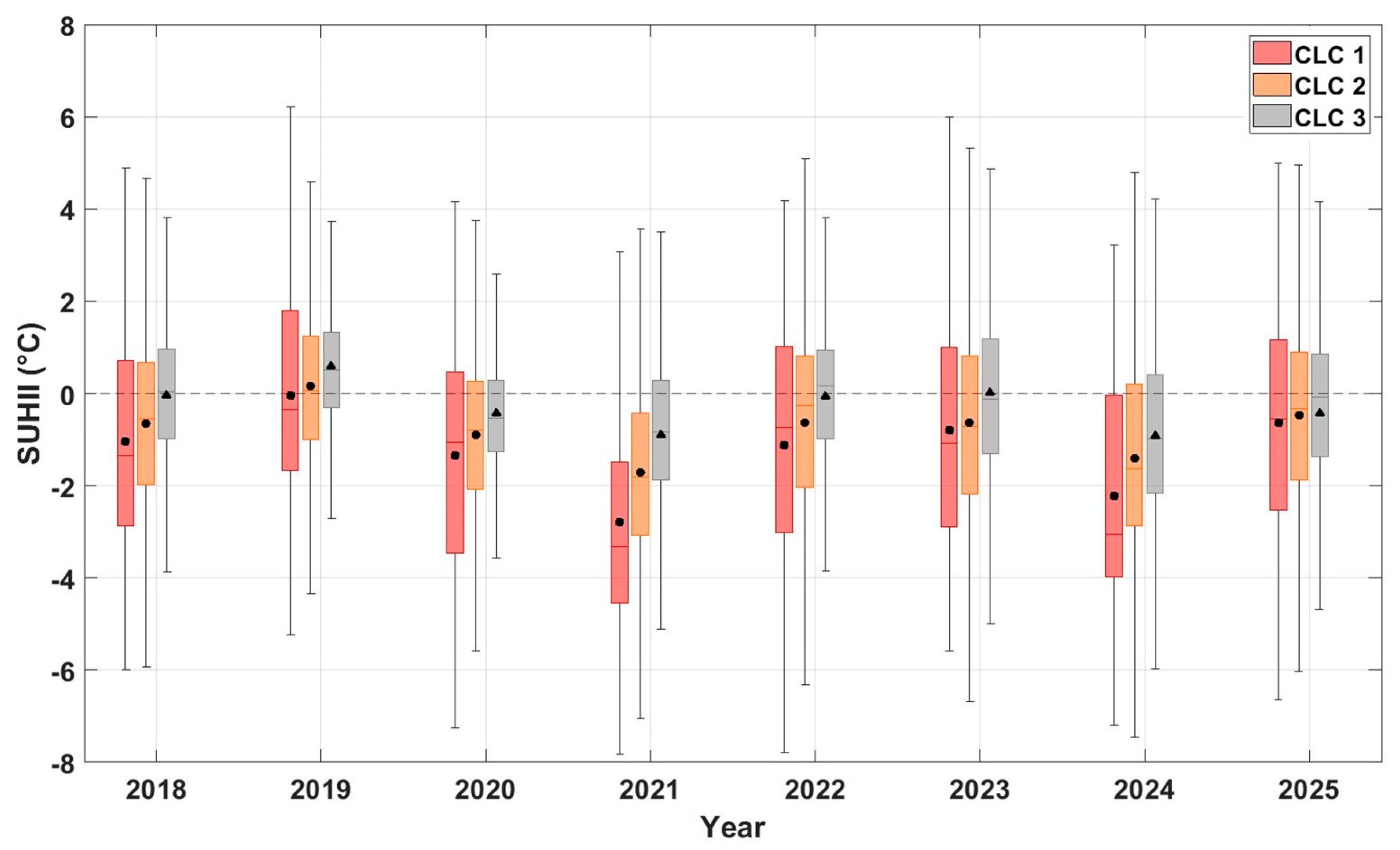
To analyze the interannual variability of summer SUHII, boxplots were generated for each CLC class (Figure 4), representing the distribution of SUHII values across different years. This graphical approach provides an effective way to identify the typical thermal conditions associated with each land cover category and to visualize the variability both within and between years.

Figure 4. SUHII variability on an annual basis for urban CLC. The black markers represent the mean values, while the red line represents the median. The dotted line indicates the value 0. The whiskers extend to ±2.7 standard deviations, encompassing 99.3% of the data.

SUHII in Lecce reveals relatively stable conditions in the period 2018–2025, with limited fluctuations from year to year and similar behavior in the three urban CLC classes. The median values of the SUHII index generally remain close to zero, indicating the prevalence of a weak or negative SUHI during summer daytime conditions. Positive anomalies occasionally appear in some years, particularly for CLC 3, but these do not exceed 2.0 °C and are not persistent over years. In contrast, the continuous (CLC 1) and discontinuous (CLC 2) urban fabric classes often show slightly negative medians, suggesting that rural areas often experience higher surface temperatures than the urban core. This result is in line with previous observations on Lecce by Donateo et al. [36] and Esposito et al. [15], who also reported negative or near–zero daytime UHI and SUHI values, attributing them to the combined effects of local ventilation, high surface reflectance, and the influence of low soil moisture. Examining the variability among the different CLC classes, CLC 1 shows the highest dispersion of SUHII values, despite its smaller and more spatially concentrated extent compared to the other urban classes. This pattern reflects the strong heterogeneity of the urban fabric and the higher temperatures that can develop in this area, as indicated by the consistently higher 75th percentile values across multiple years. In contrast, the industrial class displays lower variability, consistent with its more homogeneous structure dominated by large warehouses and impervious surfaces. Notably, this class also exhibits the highest mean SUHII values across all years, although these rarely exceed zero. Class 2, by comparison, shows intermediate variability and mean SUHII values, despite encompassing the largest and most heterogeneous urban area.

Overall, the results highlight the absence of a persistent positive SUHI signal in Lecce and suggest that thermal contrasts between urban and rural areas are mainly modulated by interannual variations in large–scale meteorological conditions rather than by changes in urban morphology or land cover type. Furthermore, the observed variability mainly reflects differences in acquisition times, highlighting the need to consider the temporal distribution of ECOSTRESS observations when comparing interannual SUHII patterns and emphasize the importance of acquisition time as a key factor controlling the observed urban–rural thermal contrast. While interannual differences highlight the combined influence of meteorological variability and acquisition timing, understanding the physical drivers of the SUHII requires a closer inspection of its diurnal cycle across land-cover classes. Therefore, the following section focuses on how different CLC categories modulate SUHII throughout the day.

3.3. SUHII Diurnal Variability in Different CLCs

This section examines the diurnal variability of SUHII in the different CLC classes by comparing the distributions of values for each time slot during the study period.

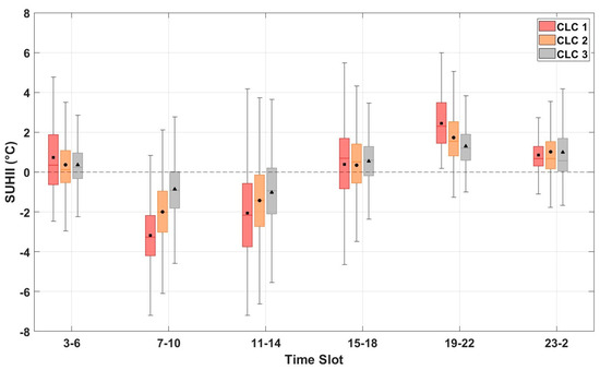
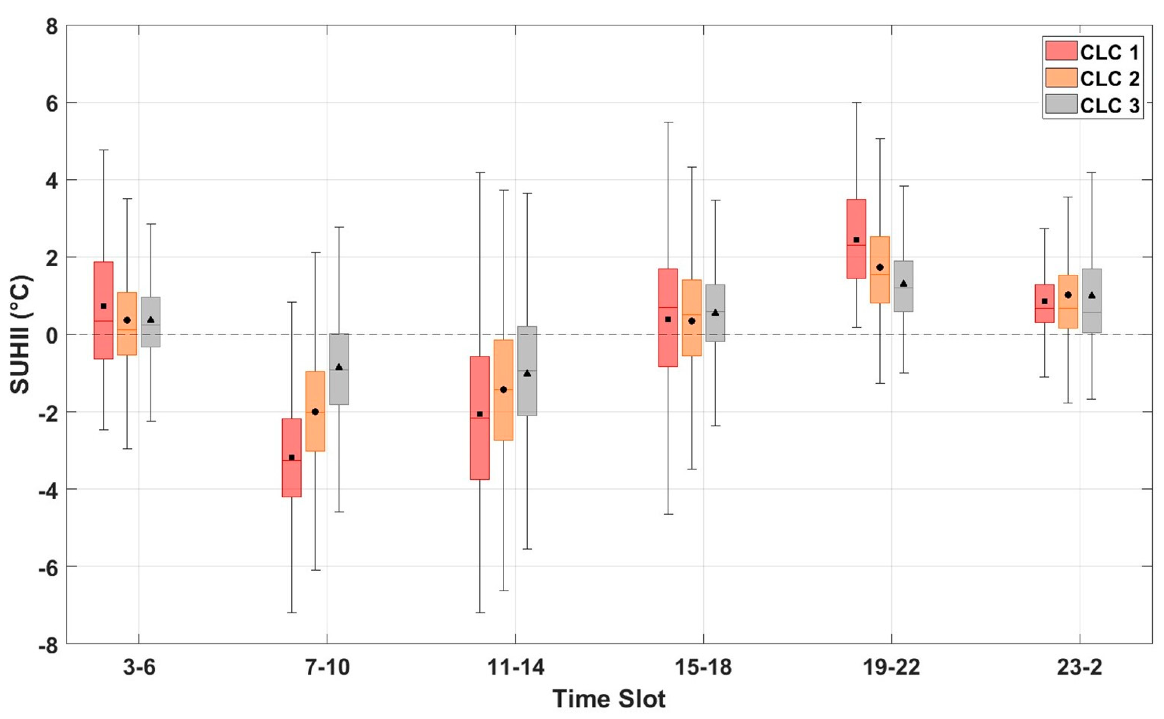
A clear diurnal pattern emerges (Figure 5), driven by solar forcing and the surface energy balance, with SUHII values transitioning from slightly positive during the early morning (03:00–06:00) to negative in the late morning and around midday (07:00–14:00), and returning to neutral or positive conditions in the afternoon and evening (15:00–02:00). In the early morning, SUHII values remain slightly positive (1.0–2.0 °C), particularly in CLC1, indicating that dense urban fabrics retain and slowly release the heat accumulated during the previous day. Following sunrise, increasing solar radiation causes a marked reduction in SUHII, reaching minimum values between 07:00 and 14:00 (−2.0 to −4.0 °C). This phase reversal highlights the faster warming of rural areas under direct solar exposure, while urban surfaces, especially in CLC1, exhibit delayed heating due to shading, higher albedo, and greater heat capacity. As observed by Esposito et al. [15], limited soil moisture in rural surroundings may further amplify this contrast. In the afternoon, SUHII gradually rises, approaching or exceeding 2.0 °C in CLC1 between 19:00 and 22:00. During late-night hours (23:00–02:00), positive anomalies persist, reflecting the delayed release of stored heat from impervious materials and the slower cooling of the urban canopy relative to vegetated rural areas.

Figure 5. Diurnal variability of SUHII for various CLC classes in the city of Lecce. Boxplot representation as in Figure 4. The whiskers extend to ±2.7 standard deviations, encompassing 99.3% of the data.

The temporal evolution of SUHII among CLC classes mirrors their morphological characteristics. CLC1 consistently exhibits the strongest nocturnal intensity and the most pronounced evening recovery, confirming the dominant role of thermal inertia associated with the high heat storage capacity of compact urban materials. Conversely, CLC3, characterized by larger open spaces and reduced shading, shows a weaker inversion and lower nocturnal SUHII values, while afternoon differences among classes tend to converge.

Overall, the SUHII diurnal cycle in Lecce confirms the alternation between a negative daytime and a positive nighttime phase. These findings are consistent with those of Esposito et al. [15] and Donateo et al. [36], who reported comparable patterns based on Sentinel-3 and in-situ observations. Similar behavior has been documented in other Mediterranean cities, such as Athens, Greece [56], where daytime SUHII values reach −2.0 °C and evening values approach 3.0 °C. Comparable trends have also been observed in arid environments, including Phoenix, Arizona (USA) [57], with daytime and nighttime intensities of −3.8 °C and +1.2 °C, respectively, as well as in Doha (Qatar) [58] and Erbil (Iraq) [59], where SUHII values remain consistently negative. Studies in Doha reported −4.8 °C during the JJA period, while those in Erbil found values ranging from −3.5 °C to −4.6 °C, attributing the negative SUHII primarily to variations in soil moisture rather than vegetation cover.

The daytime behavior observed in Lecce underscores the role of local morphological and climatic factors (such as land-cover composition, surface reflectivity, and soil moisture) in modulating the urban–rural thermal contrast.

3.4. Meteo-Climatic Characterization and Extreme Events

After characterizing both the diurnal and spatial variability of SUHII under typical summer conditions, this section now considers the broader climatic context in which these thermal patterns occur, beginning with the temporal evolution and characteristics of extreme heat events in the study period. Understanding the temporal evolution and characteristics of extreme events is essential for assessing the impacts of climate change on local and regional temperature extremes. As specified in Section 2.3 all HWs were identified using the WSDI, which provides a quantitative measure of the persistence of anomalous hot periods and is widely used to characterize heatwave events in climate studies.

It is important to note that the WSDI-based identification of extreme heat does not depend on the minimum duration criterion used to define a heatwave. Although heatwave episodes were classified in Section 2.3 following Fischer and Schär’s [49] definition of at least six consecutive days above the 90th percentile, this threshold does not influence the analyses presented here. As a result, the graphical and statistical analyses remain unaffected by the specific heatwave-duration definition.

The total number of WSDI days during the JJA season per year varies considerably, from only 7 days in 2018 to a maximum of 45 days in 2024, highlighting a general increase in the frequency and persistence of HWs over time. The summers of 2021, 2022 and 2025 also show remarkably high counts (34–39 days), indicating that prolonged and recurring WSDI episodes have become more common in recent years.

The monthly analysis shows that July has the highest overall frequency of WSDI days (86 days over the whole period), closely followed by June (81 days) and August (74 days). This distribution indicates a typical peak in WSDIs in midsummer, although significant interannual variability is evident. 2023 shows a clear predominance of July (16 days), while 2024 has an exceptional late-season peak in August (19 days). In contrast, 2025 is characterized by an early start to the season, with a record 18 WSDI days in June, indicating a possible advance in the timing of HWs events.

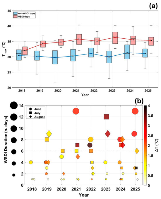
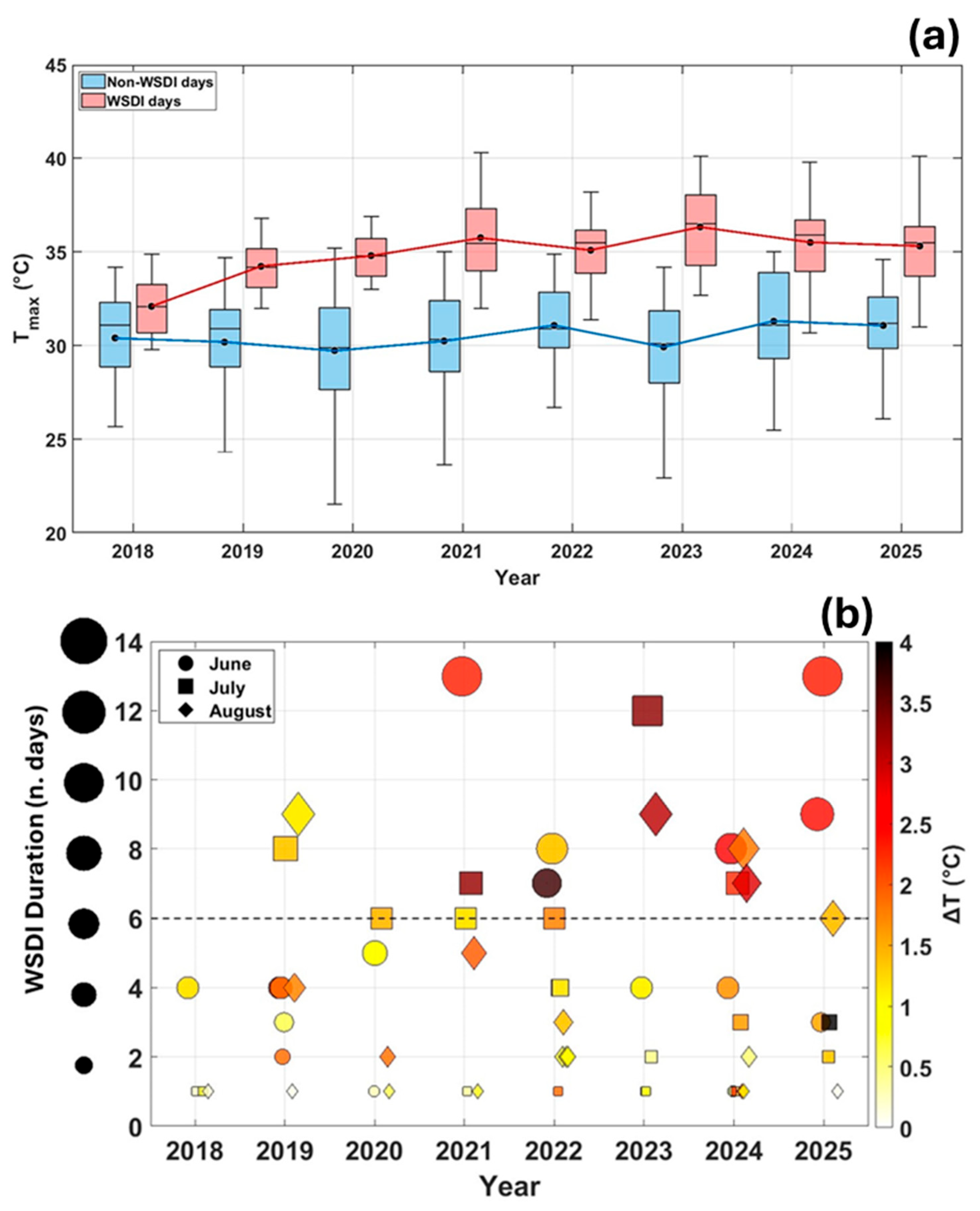
These variations in the frequency and timing of WSDI episodes are further reflected in the thermal characteristics of the events themselves, as shown in Figure 6. The graph shows the distribution of daily maximum temperatures (T_max) for WSDI (red boxes) and normal condition days (in figure referred to as non–WSDI days; blue boxes) in the years 2018–2025, during JJA season.

Figure 6. (a) Distribution of daily maximum temperature (T_max) during the JJA season for WSDI (red) and non-WSDI (blue) days. Red and blue lines indicate the mean values over the entire study period. Boxplot representation follows the same format as in Figure 5. (b) Duration and intensity of WSDI events for each summer month from 2018 to 2025. Marker size represents event duration, while color denotes the mean temperature anomaly (ΔT) relative to the 1961–1990 reference period. The dashed line marks the minimum duration required to define a heatwave event, according to Fischer and Schär [49].

As expected, temperature distributions for WSDI days are systematically higher than those for non–WSDI, confirming that the index captures periods of exceptional heat throughout years. The greater variability present in non-WSDI days is due to a larger amount of data compared to WSDI days. The mean value during WSDI days typically exceeds that of non-WSDI days by 4.0–6.0 °C, although slight variability occurs through the different years.

Interannual differences are evident: the summers of 2021 and 2023 show the highest WSDI temperatures (36.0–37.0 °C), suggesting more intense HWs, while 2020 and 2024 show slightly cooler distributions. Despite these fluctuations, the relative separation between WSDI and non–WSDI temperatures remains consistent throughout the period, reinforcing the robustness of the WSDI classification in identifying extreme summer heat events.

To assess the intensity of extreme heat events, temperature anomalies (ΔT) associated with WSDI days were calculated as the difference between the daily maximum temperature and the 90th percentile threshold for the 1961–1990 reference period (5-day window; Table 2). Between 2018 and 2020, anomalies were relatively moderate, with mean ΔT values around 1.0 °C and most WSDI days falling below the 75th percentile, while very high anomalies (above the 90th percentile) were nearly absent. From 2021 onwards, a marked shift is observed toward higher intensities, with ΔT exceeding 2.0 °C on average and a growing share of events surpassing the upper percentile thresholds. The trend culminates in 2023, which records the largest anomalies (up to 4.0–5.0 °C) and the widest variability, indicating particularly intense and persistent heatwaves.

Table 2. Percentage distribution of ΔT for WSDI days across percentile classes during JJA from 2018 to 2025.

	<P25 (0.8 °C)	P25–P75 (0.8–2.6 °C)	P75–P90 (2.6–4.1 °C)	>P90 (4.1 °C)
2018	57	43	0	0
2019	29	57	14	0
2020	33	67	0	0
2021	21	56	9	15
2022	23	62	8	8
2023	24	24	21	31
2024	22	44	27	7
2025	14	59	16	11

Overall, the progressive increase in ΔT magnitude throughout the study period highlights a clear intensification of extreme summer heat events in Lecce, consistent with the ongoing regional warming trend and the growing persistence of high-temperature conditions.

The temporal characteristics of heat events were analyzed by examining their duration and seasonal distribution (Figure 6b). Each symbol represents a WSDI episode identified in a given summer month for each year, with symbol size proportional to event duration (consecutive WSDI days) and color indicating the corresponding mean intensity (ΔT).

The graph highlights a marked interannual variability in both duration and intensity. Before 2020, heat events were generally shorter and milder, typically lasting 2–5 days with ΔT < 2.0 °C. From 2021 onwards, longer and more intense heatwaves became more frequent, with several persistent episodes in 2023 and 2025 lasting 8–10 days and reaching ΔT values above 3.0 °C. The color scale confirms that prolonged events are associated with higher ΔT, indicating a concurrent increase in both intensity and persistence of extreme summer heatwaves.

Seasonally, July and August record the longest and most intense events, whereas June shows comparatively weaker anomalies. The increasing duration and intensity of heatwaves in recent years demonstrate a clear amplification of extreme summer conditions.

3.5. Correlation Between Extreme Heat Events and SUHII

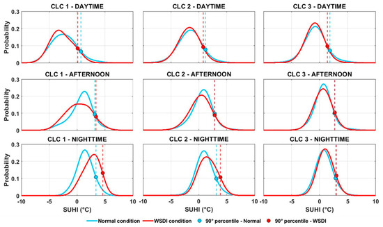
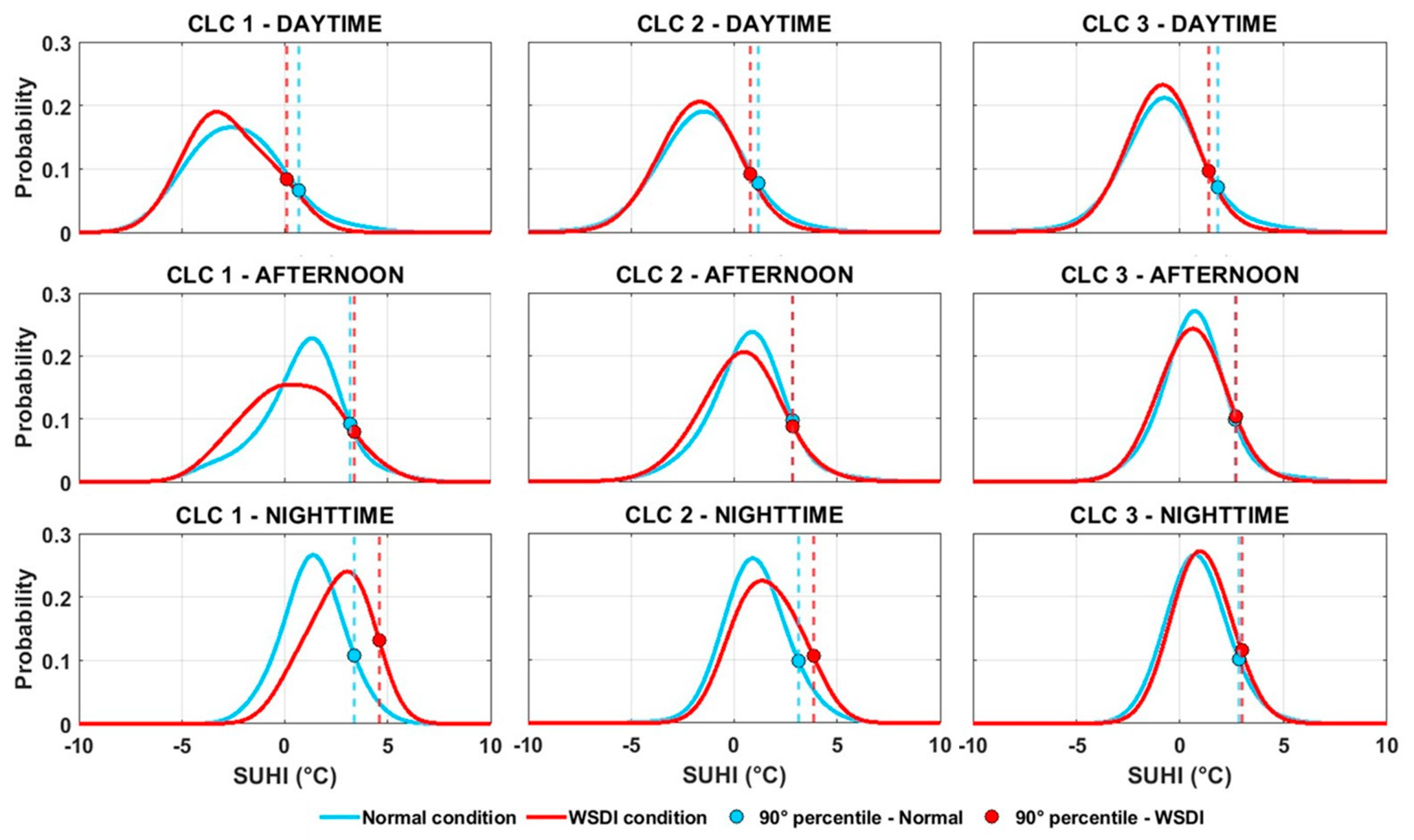
Given the increasing frequency and intensity of HWs identified through the WSDI, it is essential to quantify how these extreme conditions affect the urban-rural thermal contrast. This section therefore assesses the response of the SUHII under WSDI conditions compared to normal conditions. To assess the impact of WSDI on SUHII, an analysis was performed across three periods of the day and for three urban classes (Figure 7). The probability distribution of SUHII was calculated for both WSDI and normal conditions to capture differences across the entire CLC domain under varying climatic regimes. To examine diurnal variability, the dataset was divided into three-time intervals: daytime (06:00–14:00), afternoon (15:00–19:00), and nighttime (20:00–05:00).

Figure 7. PDFs of SUHII under normal (blue) and WSDI (red) conditions for three urban classes (CLC 1–3) across daytime, afternoon, and nighttime. Dashed lines indicate 90th percentiles of SUHII distribution.

The probability density functions (PDFs) for each CLC class were then analyzed and compared to evaluate how SUHII responds to WSDI conditions. Similar approaches based on kernel density estimation and SUHI distributional analysis have been employed in previous studies to investigate LST variability under different climatic or morphological contexts (e.g., Taheri Shahraiyni et al. [60]).

Quantitatively, during the daytime interval, WSDI conditions lead to a marked shift towards more negative SUHII values of approximately −1.1 °C in compact tissues (CLC 1) and more moderate shifts in CLC 2 and CLC 3 (approximately −0.7 °C) compared to normal conditions. In contrast, during the night, SUHII intensifies positively under WSDI conditions, increasing by approximately 2.6 °C in CLC 1, 1.6 °C in CLC 2 and 0.3 °C in CLC 3. These values correspond to the shift in peak distribution between WSDI and normal conditions. Also, these changes quantify the greater daytime rural warming and stronger nighttime heat retention characteristic of extreme heat events.

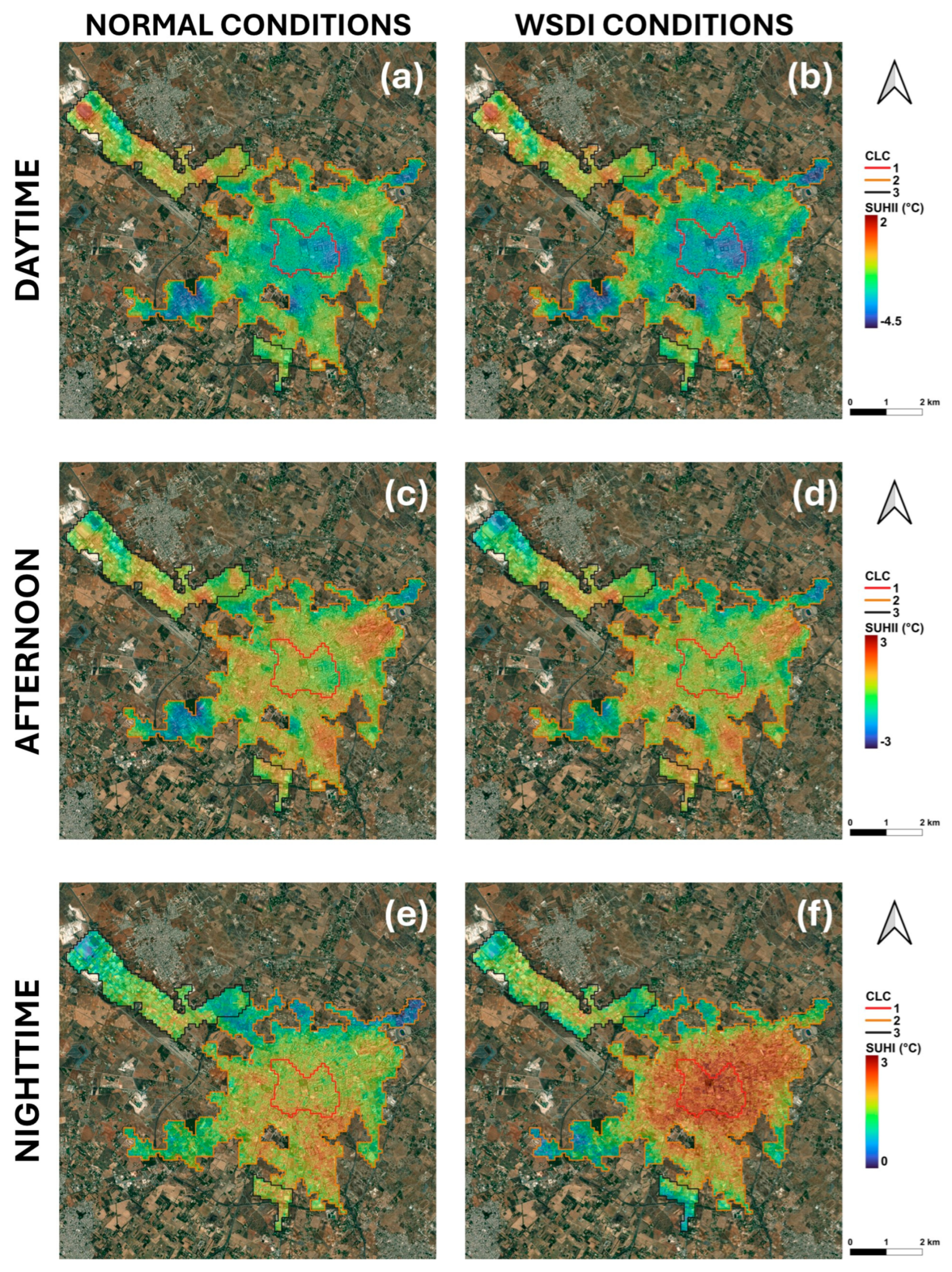
The analysis of SUHII distributions under normal and WSDI conditions (Figure 8) reveals distinct and statistically significant differences across the three CLC classes. During the day and afternoon, WSDI distributions generally shift toward lower SUHII values, indicating a reinforcement of the daytime cool island effect. Conversely, at night, distributions move toward higher SUHII values, revealing enhanced heat retention and a stronger nocturnal heat island during WSDI periods.

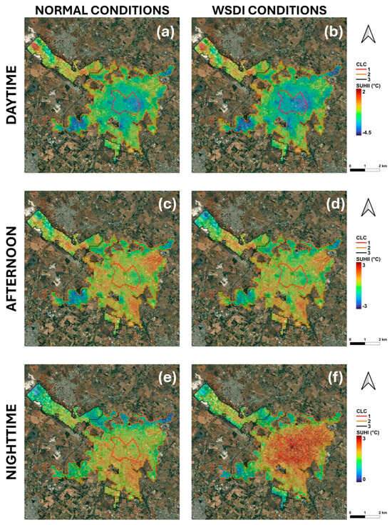
Figure 8. Mean SUHII (2018–2025) maps across the three-time intervals for the city of Lecce in normal conditions (a,c,e) and under WSDI conditions (b,d,f).

In CLC 1, the probability distributions display a clear diurnal asymmetry. During the day and afternoon, the curves shift to the left, suggesting less intense SUHII values and an apparent intensification of the cool island effect under WSDI conditions. The shapes of the distributions remain similar, although WSDI days show a higher probability of negative anomalies, consistent with previous findings (e.g., [15]). However, despite this relative cooling, the absolute air and surface temperatures remain significantly higher during heatwave periods, meaning that overall thermal stress during central hours is still greater. At night, the WSDI distribution shifts markedly toward higher SUHI values, with a broader, asymmetric shape indicative of enhanced heat storage and increased probability of extreme nocturnal conditions.

For CLC 2, the distributions reveal a more moderate response. During the day and afternoon, the curves retain similar shapes, but a slight leftward shift under WSDI conditions indicates a weaker cool island effect compared to CLC 1. Yet, as in denser urban areas, this apparent cooling does not translate into improved comfort, since overall temperatures are still elevated during heatwave events. At night, the WSDI curve shifts toward higher SUHI values, with a broader tail toward extremes, showing that even in moderately dense fabrics, thermal accumulation and nighttime heat release intensify during WSDI periods.

In CLC 3, the daytime distributions show only marginal differences between normal and WSDI conditions, reflecting limited enhancement of the cool island effect. The nighttime WSDI distribution shifts slightly toward higher SUHI values, indicating a modest increase in heat retention. These small variations reflect the higher permeability and better ventilation typical of this class, which mitigate part of the nighttime warming but not the overall heat exposure.

Both the Mann–Whitney U test [61,62] and Welch’s t-test [63,64] yield p-values < 0.05 for all classes and time intervals, confirming that the differences between normal and WSDI conditions are statistically significant.

Overall, the diurnal evolution of SUHII reveals a progressive reversal in thermal behavior under WSDI conditions: stronger daytime cooling relative to rural surroundings and intensified nocturnal warming. The amplitude of this asymmetry increases with urban density, being most pronounced in compact fabrics (CLC 1). Nevertheless, even where a more intense cool island is detected, this effect is largely negligible in terms of actual thermal stress, as the higher baseline temperatures during WSDI conditions outweigh any relative cooling.

These results highlight an important limitation in interpreting SUHI intensity as a proxy for urban thermal stress and outdoor comfort. As also discussed by Martilli et al. [35], focusing solely on the urban–rural temperature contrast may obscure the fact that both urban and rural areas experience elevated absolute temperatures during heatwaves. Therefore, SUHI alone is not sufficient to assess the real impact of extreme heat on urban livability or to evaluate the effectiveness of potential mitigation strategies.

Figure 8 shows the average SUHII values during WSDI and normal condition days across the three time periods defined in the previous analysis. During the daytime (Figure 8a,b), all urban classes exhibit more negative SUHII under WSDI conditions, consistent with the probability distributions shown in Figure 7. The reduction is most pronounced in compact urban areas, moderate in intermediate fabrics, and marginal in less dense zones. However, this apparent intensification of the cool island effect does not indicate actual cooling of urban surfaces but rather a faster and more intense warming of rural surroundings, where prolonged heat and soil dryness reduce evaporative cooling. Consequently, despite a more negative SUHII, overall thermal stress during central hours remains higher. This behavior, particularly evident in dense and intermediate fabrics, aligns with previous studies reporting an attenuation or even reversal of the daytime SUHI during heatwave periods [65,66,67].

In the afternoon (Figure 8c,d), this pattern persists but with smaller magnitude. SUHII values remain slightly negative or nearly neutral, suggesting that the accumulated daytime heat is not yet sufficient to generate strong contrasts between built-up and non-urban areas.

During the nighttime (Figure 8e,f), the pattern reverses: SUHII intensifies markedly under WSDI conditions, highlighting the accumulation and delayed release of heat stored in urban materials. The increase is strongest in compact fabrics and diminishes with lower building density. This nocturnal amplification reflects the higher thermal inertia and reduced cooling efficiency typical of dense urban morphologies. Similar findings were reported by Cheval et al. [65], Rech et al. [66], and Zhao et al. [67], who observed systematic nighttime SUHI intensification during heatwave events across different urban contexts. Li and Bou-Zeid [68] further described this behavior as a synergistic interaction between urban heat islands and heatwaves, where their combined effect on nighttime temperatures exceeds the sum of their individual contributions. Satellite analyses corroborate this trend: Shi et al. [69] demonstrated that urbanization amplifies nighttime heatwave intensity across China, while Sarangi et al. [70] reported similar findings for U.S. cities.

Comparable results were also observed in Lecce and Milan by Esposito et al. [15]: in Lecce, SUHII reached its most negative daytime values due to rural heating under low soil-moisture conditions, while in Milan, nighttime SUHI intensity increased during heatwaves. Buyantuyev and Wu [71] similarly emphasized that land-cover heterogeneity drives strong spatial contrasts, with rural areas experiencing greater daytime heating under drought. Li et al. [72] demonstrated that urban density and morphology modulate SUHII primarily through differences in thermal inertia, confirming that the apparent daytime “cooling” of urban areas during extreme events is a relative effect driven by large-scale surface energy exchanges.

Overall, both statistical and spatial analyses reveal a consistent pattern: stronger negative SUHII during the day and a pronounced nighttime intensification under WSDI conditions. This dual behavior underscores the fundamental role of urban morphology and material thermal properties in modulating local heat accumulation. It also highlights the limitations of SUHI as a standalone indicator of urban heat stress and comfort, since absolute temperatures, not relative contrasts, determine the real impact of heat extremes and the effectiveness of mitigation strategies.

4. Conclusions

This study provides a comprehensive assessment of the spatiotemporal dynamics of SUHII intensity and its response to extreme heat conditions in Lecce (south–east Italy) during the summers from 2018 to 2025. By combining high-resolution ECOSTRESS thermal data with the WSDI index, the analysis offers new insights into how urban and rural surfaces respond to extreme summer conditions in a Mediterranean environment.

The results reveal that Lecce is characterized by a predominantly negative daytime SUHII, indicating that rural areas generally heat up more quickly and intensely than the urban center during dry, highly irradiated summer days. This behavior does not necessarily suggest an intrinsic cooling capacity of the city, but rather reflects the greater rural heating associated with low soil moisture and limited evaporative cooling in the surrounding agricultural areas. The diurnal cycle shows a systematic reversal, with negative SUHII values during the day and positive values at night, reflecting the alternation between daytime rural warming and nighttime urban heat retention due to the greater thermal inertia of building materials. Overall, the results indicate that Lecce’s apparent daytime “coolness” is a relative effect resulting from stronger rural warming, while nighttime thermal persistence is accentuated by the city’s morphology and material composition.

Analysis of extreme heat dynamics reveals a progressive intensification of both the frequency and persistence of extreme events, particularly after 2020, with the most extreme conditions observed in 2023 and 2025. Under HW conditions as defined by the WSDI, the SUHII shows a marked diurnal asymmetry: daytime SUHIIs become more negative due to accelerated warming in rural areas, while nighttime intensities increase significantly as urban materials slowly retain and release stored heat. This pattern is most evident in compact, densely built-up areas (CLC 1), where reduced ventilation and increased thermal inertia amplify the persistence of nighttime heat. The increasing intensity and persistence of HW events further highlight the contrasting thermal behavior of urban and rural environments under extreme conditions. These results highlight the importance of considering both soil moisture dynamics and surface energy exchanges in interpreting urban thermal responses in Mediterranean contexts.

In addition to climate results, this study also demonstrates the strong potential of ECOSTRESS for urban climate monitoring. The sensor’s high spatial resolution and variable overflight times allow it to detect small-scale diurnal temperature variations that cannot be captured by traditional sensors such as LANDSAT, MODIS or Sentinel-3. ECOSTRESS therefore offers unique opportunities to characterize the intra-diurnal evolution of urban surface temperatures, identify local microclimatic patterns, and quantify the response of urban and rural surfaces to short-duration extreme events such as heatwaves. When combined with long-term climate indicators such as the WSDI, ECOSTRESS data can bridge the gap between local thermal processes and broader climate trends, supporting both research and urban climate adaptation planning.

Despite the advantages of combining multi-year ECOSTRESS observations with CLC-based land cover information and long-term climate indices, certain limitations must be acknowledged. First, the irregular orbital pattern of the ISS results in an uneven temporal distribution of ECOSTRESS acquisitions, particularly during the night, which may limit the representation of night-time SUHII variability. Although a multi-year dataset mitigates this problem, the temporal imbalance cannot be completely eliminated. Second, SUHII is based on satellite-derived surface temperatures and does not take into account near-surface air temperature or human thermal comfort, implying that SUHI intensity should not be interpreted as a direct indicator of heat stress. Third, although the rural reference class was carefully defined using CLC+ Backbone data, some residual variability in rural land covers may still affect daytime thermal contrasts. Moreover, biophysical variables such as soil moisture or albedo were not explicitly included, as the study focuses primarily on SUHII derived from ECOSTRESS observations and land-cover classes. Finally, while Lecce is representative of medium-sized Mediterranean cities, the results should be interpreted within this specific climatic and morphological context.

From an applied perspective, the study underscores the value of high-resolution satellite thermal observations for assessing urban vulnerability and guiding adaptation strategies. Expanding the use of sensors such as ECOSTRESS, together with model-based and ground-data-based approaches, can improve our understanding of urban heat processes and support the design of climate-resilient cities through the integration of green infrastructure, reflective materials, and ventilation corridors aimed at mitigating nighttime heat accumulation.

References

- Donateo, A.; Dinoi, A.; Pappaccogli, G. Impact on Ultrafine Particles Concentration and Turbulent Fluxes of SARS-CoV-2 Lockdown in a Suburban Area in Italy. Atmosphere 2021, 12, 407. [Google Scholar]
- Oke, T.R. Urban Climates and Global Environmental Change. In Applied Climatology: Principles & Practices; Thompson, R.D., Perry, A., Eds.; Routledge: London, UK, 1997; pp. 273–287. [Google Scholar]
- Founda, D.; Santamouris, M. Synergies between Urban Heat Island and Heat Waves in Athens (Greece), during an extremely hot summer (2012). Sci. Rep. 2017, 7, 10973. [Google Scholar] [CrossRef] [Scilit]
- Giannaros, T.M.; Melas, D. Study of the Urban Heat Island in a Coastal Mediterranean City: The Case Study of Thessaloniki, Greece. Atmos. Res. 2012, 118, 103–120. [Google Scholar] [CrossRef] [Scilit]
- Rajagopal, P.; Priya, R.S.; Senthil, R. A Review of Recent Developments in the Impact of Environmental Measures on Urban Heat Island. Sustain. Cities Soc. 2023, 88, 104279. [Google Scholar] [CrossRef] [Scilit]
- Gill, S.E.; Handley, J.F.; Ennos, A.R.; Pauleit, S. Adapting cities for climate change: The role of the green infrastructure. Built Environ. 2007, 33, 115–133. [Google Scholar] [CrossRef] [Scilit]
- CORINE Land Cover 2018 (Raster 100 m), Europe, 6-Yearly—Version 2020_20u1, May 2020; EEA: Copenhagen, Denmark, 2020. [CrossRef]
- Copernicus. Available online: https://land.copernicus.eu/content/corine-land-cover-nomenclature-guidelines/html/ (accessed on 1 December 2025).
- Leconte, F.; Bouyer, J.; Claverie, R.; Pétrissans, M. Using local climate zone scheme for UHI assessment: Evaluation of the method using mobile measurements. Build. Environ. 2015, 83, 39–49. [Google Scholar] [CrossRef] [Scilit]
- Lin, Y.; Jim, C.Y.; Deng, J.; Wang, Z. Urbanization effect on spatiotemporal thermal patterns and changes in Hangzhou (China). Build. Environ. 2018, 145, 166–176. [Google Scholar] [CrossRef] [Scilit]
- Yan, C.; Guo, Q.; Li, H.; Li, L.; Qiu, G.Y. Quantifying the cooling effect of urban vegetation by mobile traverse method: A local-scale urban heat island study in a subtropical megacity. Build. Environ. 2020, 169, 106541. [Google Scholar] [CrossRef] [Scilit]
- Martilli, A.; Sánchez, B.; Santiago, J.L.; Rasilla, D.; Pappaccogli, G.; Allende, F.; Martín, F.; Roman-Cascón, C.; Yagüe, C.; Fernández, F. Simulating the Pollutant Dispersion during Persistent Wintertime Thermal Inversions over Urban Areas: The Case of Madrid. Atmos. Res. 2022, 270, 106058. [Google Scholar]
- Zhou, D.; Xiao, J.; Bonafoni, S.; Berger, C.; Deilami, K.; Zhou, Y.; Frolking, S.; Yao, R.; Qiao, Z.; Sobrino, J.A. Satellite Remote Sensing of Surface Urban Heat Islands: Progress, Challenges, and Perspectives. Remote Sens. 2019, 11, 48. [Google Scholar]
- Naserikia, M.; Hart, M.A.; Nazarian, N.; Bechtel, B.; Lipson, M.; Nice, K.A. Land Surface and Air Temperature Dynamics: The Role of Urban Form and Seasonality. Sci. Total Environ. 2023, 905, 167306. [Google Scholar] [CrossRef] [Scilit]
- Esposito, A.; Pappaccogli, G.; Donateo, A.; Salizzoni, P.; Maffeis, G.; Semeraro, T.; Santiago, J.L.; Buccolieri, R. Urban Morphology and Surface Urban Heat Island Relationship During Heat Waves: A Study of Milan and Lecce (Italy). Remote Sens. 2024, 16, 4496. [Google Scholar] [CrossRef] [Scilit]
- Pinker, R.T.; Ma, Y.; Chen, W.; Hulley, G.; Borbas, E.; Islam, T.; Hain, C.; Cawse-Nicholson, K.; Hook, S.; Basara, J. Towards a unified and coherent land surface temperature earth system data record from geostationary satellites. Remote Sens. 2019, 11, 1399. [Google Scholar] [CrossRef] [Scilit]
- Wu, Z.; Yao, L.; Ren, Y. Characterizing the spatial heterogeneity and controlling factors of land surface temperature clusters: A case study in Beijing. Build. Environ. 2020, 169, 106598. [Google Scholar] [CrossRef] [Scilit]
- Geletič, J.; Lehnert, M.; Savić, S.; Milošević, D. Inter-/intra-zonal seasonal variability of the surface urban heat island based on local climate zones in three central European cities. Build. Environ. 2019, 156, 21–32. [Google Scholar] [CrossRef] [Scilit]
- Wang, C.; Middel, A.; Myint, S.W.; Kaplan, S.; Brazel, A.J.; Lukasczyk, J. Assessing local climate zones in arid cities: The case of Phoenix, Arizona and Las Vegas, Nevada. ISPRS J. Photogramm. Remote Sens. 2018, 141, 59–71. [Google Scholar] [CrossRef] [Scilit]
- Hulley, G. ECOsystem Spaceborne Thermal Radiometer Experiment on Space Station (ECOSTRESS) Mission–Level 2 Product User Guide; LP DAAC: Sioux Falls, SD, USA, 2019.
- Chang, Y.; Xiao, J.; Li, X.; Middel, A.; Zhang, Y.; Gu, Z.; He, S. Exploring diurnal thermal variations in urban local climate zones with ECOSTRESS land surface temperature data. Remote Sens. Environ. 2021, 263, 112544. [Google Scholar] [CrossRef] [Scilit]
- Chang, Y.; Xiao, J.; Li, X.; Weng, Q. Monitoring diurnal dynamics of surface urban heat island for urban agglomerations using ECOSTRESS land surface temperature observations. Sustain. Cities Soc. 2023, 98, 104833. [Google Scholar] [CrossRef] [Scilit]
- Hulley, G.; Shivers, S.; Wetherley, E.; Cudd, R. New ECOSTRESS and MODIS Land Surface Temperature Data Reveal Fine-Scale Heat Vulnerability in Cities: A Case Study for Los Angeles County, California. Remote Sens. 2019, 11, 2136. [Google Scholar] [CrossRef] [Scilit]
- Wei, L.; Sobrino, J.A. Surface urban heat island analysis based on local climate zones using ECOSTRESS and Landsat data: A case study of Valencia city (Spain). Int. J. Appl. Earth Obs. Geoinf. 2024, 130, 103875. [Google Scholar] [CrossRef] [Scilit]
- Pappaccogli, G.; Esposito, A.; Buccolieri, R. Summer Diurnal LST Variability Across Local Climate Zones Using ECOSTRESS Data in Lecce and Milan. Atmosphere 2025, 16, 377. [Google Scholar] [CrossRef] [Scilit]
- Yao, R.; Huang, X.; Zhang, Y.; Wang, L.; Li, J.; Yang, Q. Estimation of the Surface Urban Heat Island Intensity Across 1031 Global Cities Using the Regression-Modification-Estimation (RME) Method. J. Clean. Prod. 2024, 434, 140231. [Google Scholar] [CrossRef] [Scilit]
- Stathopoulou, M.; Cartalis, C. Daytime urban heat islands from Landsat ETM+ and Corine land cover data: An application to major cities in Greece. Sol. Energy 2007, 81, 358–368. [Google Scholar] [CrossRef] [Scilit]
- Stamou, A.; Dosiou, A.; Bakousi, A.; Karachaliou, E.; Tavantzis, I.; Stylianidis, E. Assessing Spatial Correlations Between Land Cover Types and Land Surface Temperature Trends Using Vegetation Index Techniques in Google Earth Engine: A Case Study of Thessaloniki, Greece. Remote Sens. 2025, 17, 403. [Google Scholar] [CrossRef] [Scilit]
- García, D.H. Analysis and precision of the Terrestrial Surface Temperature using Landsat 8 and Sentinel 3 images: Study applied to the city of Granada (Spain). Sustain. Cities Soc. 2021, 71, 102980. [Google Scholar] [CrossRef] [Scilit]
- Albini, G.; Guerri, G.; Munafò, M.; Morabito, M. Investigation of the Surface Urban Heat Island (SUHI) by two remote sensing-based approaches in Italian regional capitals. Remote Sens. Appl. Soc. Environ. 2025, 38, 101567. [Google Scholar] [CrossRef] [Scilit]
- Hellings, A.; Rienow, A. Mapping Land Surface Temperature Developments in Functional Urban Areas across Europe. Remote Sens. 2021, 13, 2111. [Google Scholar] [CrossRef] [Scilit]
- Renc, A.; Łupikasza, E.; Błaszczyk, M. Spatial structure of the surface heat and cold islands in summer based on Landsat 8 imagery in southern Poland. Ecol. Indicat. 2022, 142, 109181. [Google Scholar]
- Sfîcă, L.; Corocăescu, A.-C.; Crețu, C.-Ș.; Amihăesei, V.-A.; Ichim, P. Spatiotemporal Features of the Surface Urban Heat Island of Bacău City (Romania) during the Warm Season and Local Trends of LST Imposed by Land Use Changes during the Last 20 Years. Remote Sens. 2023, 15, 3385. [Google Scholar] [CrossRef] [Scilit]
- Naeem, S.; Mahmood, S.A. Exploring the Nexus between LULC Transformation, Land Surface Temperature, and Drought in a Rapidly Urbanizing Landscape: The Case of Multan. DYSONA Appl. Sci. 2026, 7, 98–109. [Google Scholar] [CrossRef] [Scilit]
- Martilli, A.; Krayenhoff, E.S.; Nazarian, N. Is the urban heat island intensity relevant for heat mitigation studies? Urban Clim. 2020, 31, 100541. [Google Scholar] [CrossRef] [Scilit]
- Donateo, A.; Palusci, O.; Pappaccogli, G.; Esposito, A.; Martilli, A.; Santiago, J.L.; Buccolieri, R. Analysis of urban heat island and human thermal comfort in a Mediterranean city: A case study of Lecce (Italy). Sustain. Cities Soc. 2023, 98, 104849. [Google Scholar] [CrossRef] [Scilit]
- Emmanuel, R.; Krüger, E. Urban heat island and its impact on climate change resilience in a shrinking city: The case of Glasgow, UK. Build. Environ. 2012, 53, 137–149. [Google Scholar] [CrossRef] [Scilit]
- ISTAT. Popolazione Residente al 1° Gennaio 2025, Comune, Lecce. 2025. Available online: https://demo.istat.it/app/?l=en&a=2025&i=POS (accessed on 1 December 2025).
- Esposito, A.; Grulois, M.; Pappaccogli, G.; Palusci, O.; Donateo, A.; Salizzoni, P.; Santiago, J.L.; Martilli, A.; Maffeis, G.; Buccolieri, R. On the calculation of urban morphological parameters using GIS: An application to Italian cities. Atmosphere 2023, 14, 329. [Google Scholar] [CrossRef] [Scilit]
- Giorgi, F.; Lionello, P. Climate change projections for the Mediterranean region. Glob. Planet. Chang. 2008, 63, 90–104. [Google Scholar] [CrossRef] [Scilit]
- Martano, P.; Elefante, C.; Grasso, F. Ten years water and energy surface balance from the CNR-ISAC micrometeorological station in Salento peninsula (southern Italy). Adv. Sci. Res. 2015, 12, 121–125. [Google Scholar] [CrossRef] [Scilit]
- Donateo, A.; Conte, M.; Grasso, F.M.; Contini, D. Seasonal and diurnal behaviour of size segregated particles fluxes in a suburban area. Atmos. Environ. 2019, 219, 117. [Google Scholar] [CrossRef] [Scilit]
- Hook, S.J.; Cawse-Nicholson, K.; Barsi, J.; Radocinski, R.; Hulley, G.C.; Johnson, W.R.; Rivera, G.; Markham, B. In-flight validation of the ECOSTRESS, Landsats 7 and 8 thermal infrared spectral channels using the Lake Tahoe CA/NV and Salton Sea CA automated validation sites. IEEE Trans. Geosci. Remote Sens. 2020, 58, 1294–1302. [Google Scholar] [CrossRef]
- Hulley, G.C.; Gottsche, F.M.; Rivera, G.; Hook, S.J.; Freepartner, R.J.; Martin, M.A.; Cawse-Nicholson, K.; Johnson, W.R. Validation and Quality Assessment of the ECOSTRESS Level-2 Land Surface Temperature and Emissivity Product. IEEE Trans. Geosci. Remote Sens. 2022, 60, 5000523. [Google Scholar] [CrossRef] [Scilit]
- Dunn, R.J.; Alexander, L.V.; Donat, M.G.; Zhang, X.; Bador, M.; Herold, N.; Lippmann, T.; Allan, R.; Aguilar, E.; Barry, A.A.; et al. Development of an updated global land in situ-based data set of temperature and precipitation extremes: HadEX3. J. Geophys. Res. Atmos. 2020, 125, e2019JD032263. [Google Scholar] [CrossRef] [Scilit]
- Barriopedro, D.; García-Herrera, R.; Ordóñez, C.; Miralles, D.G.; Salcedo-Sanz, S. Heat waves: Physical understanding and scientific challenges. Rev. Geophys. 2023, 61, e2022RG000780. [Google Scholar] [CrossRef] [Scilit]
- Pappaccogli, G.; Giangrande, F.; Esposito, A.; Donateo, A.; Lionello, P.; Buccolieri, R. Dynamics of urban heat island intensity in Lecce, Italy: Seasonal, diurnal and heat wave influence. Bull. Atmos. Sci. Technol. 2024, 5, 8. [Google Scholar] [CrossRef] [Scilit]
- Hussain, M.M.; Mahmud, I.; Bari, S.H. pyHomogeneity: A Python Package for Homogeneity Test of Time Series Data. J. Open Res. Softw. 2023, 11, 4. [Google Scholar] [CrossRef] [Scilit]
- Fischer, E.; Schär, C. Consistent geographical patterns of changes in high-impact European heatwaves. Nat. Geosci. 2010, 3, 398–403. [Google Scholar] [CrossRef] [Scilit]
- Esposito, A.; Pappaccogli, G.; Bozzeda, F.; Buccolieri, R. A multi-city statistical modelling of surface urban heat island: Application to Italian cities. Urban Clim. 2025, 64, 102717. [Google Scholar] [CrossRef] [Scilit]
- Guarino, M.V.; Martilli, A.; Di Sabatino, S.D.; Leo, L.S. Modelling the Urban Boundary-Layer over a Typical Mediterranean City Using Wrf: Assessment of Uhi and Thermal Comfort; American Society of Mechanical Engineers: New York, NY, USA, 2004; pp. 304–307. [Google Scholar]
- Johansson, E. Influence of urban geometry on outdoor thermal comfort in a hot dry climate: A study in Fez, Morocco. Build. Environ. 2006, 41, 1326–1338. [Google Scholar] [CrossRef] [Scilit]
- Touchaei, A.G.; Akbari, H. Evaluation of the seasonal effect of increasing the albedo on urban climate and energy consumption of buildings in Montreal. Urban Clim. 2015, 14, 278–289. [Google Scholar] [CrossRef] [Scilit]
- Touchaei, A.G.; Hosseini, M.; Akbari, H. Energy savings potentials of commercial buildings by urban heat island reduction strategies in Montreal (Canada). Energy Build. 2016, 110, 41–48. [Google Scholar] [CrossRef] [Scilit]
- Touchaei, A.G.; Wang, Y. Characterizing urban heat island in Montreal (Canada)—Effect of urban morphology. Sustain. Cities Soc. 2015, 19, 395–402. [Google Scholar] [CrossRef] [Scilit]
- Stathopoulou, M.; Constantinos, C. Study of the urban heat island of Athens, Greece during daytime and night-time. In Proceedings of the 2007 Urban Remote Sensing Joint Event, Paris, France, 11–13 April 2007. [Google Scholar]
- Hartz, D.A.; Prashad, L.; Hedquist, B.C.; Golden, J.; Brazel, A.J. Linking satellite images and hand-held infrared thermography to observed neighborhood climate conditions. Remote Sens. Environ. 2006, 104, 190–200. [Google Scholar] [CrossRef] [Scilit]
- Rajeswari, J.R.; Fountoukis, C.; Siddique, A.; Moosakutty, S.; Mohieldeen, Y.; Ayoub, M.A.; Alfarra, M.R. Urban heat island phenomenon in a desert, coastal city: The impact of urbanization. Urban Clim. 2024, 56, 102016. [Google Scholar] [CrossRef] [Scilit]
- Rasul, A.; Balzter, H.; Smith, C. Spatial variation of the daytime surface urban cool island during the dry season in Erbil, Iraqi Kurdistan, from Landsat 8. Urban Clim. 2015, 14, 176–186. [Google Scholar] [CrossRef] [Scilit]
- Taheri Shahraiyni, H.; Sodoudi, S.; El-Zafarany, A.; Abou El Seoud, T.; Ashraf, H.; Krone, K. A Comprehensive Statistical Study on Daytime Surface Urban Heat Island During Summer in Urban Areas, Case Study: Cairo and Its New Towns. Remote Sens. 2016, 8, 643. [Google Scholar] [CrossRef] [Scilit]
- Mann, H.B.; Whitney, D.R. On a Test of Whether One of Two Random Variables is Stochastically Larger than the Other. Ann. Math. Statist. 1947, 18, 50–60. [Google Scholar] [CrossRef] [Scilit]
- Hollander, M.; Wolfe, D.A.; Chicken, E. Nonparametric Statistical Methods, 3rd ed.; Wiley: Hoboken, NJ, USA, 2014. [Google Scholar]
- Welch, B.L. The Generalization of “Student’s” Problem When Several Different Population Variances Are Involved. Biometrika 1947, 34, 28–35. [Google Scholar] [CrossRef] [Scilit]
- Ruxton, G.D. The Unequal Variance t-Test Is an Underused Alternative to Student’s t-Test and the Mann–Whitney U Test. Behav. Ecol. 2006, 17, 688–690. [Google Scholar] [CrossRef] [Scilit]
- Cheval, S.; Amihăesei, V.-A.; Chitu, Z.; Dumitrescu, A.; Falcescu, V.; Irașoc, A.; Micu, D.M.; Mihulet, E.; Ontel, I.; Paraschiv, M.-G.; et al. A Systematic Review of Urban Heat Island and Heat Waves Research (1991–2022). Clim. Risk Manag. 2024, 44, 100603. [Google Scholar] [CrossRef] [Scilit]
- Rech, B.; Moreira, R.N.; Mello, T.A.G.; Klouček, T.; Komárek, J. Assessment of Daytime and Nighttime Surface Urban Heat Islands across Local Climate Zones—A Case Study in Florianópolis, Brazil. Urban Clim. 2024, 55, 101954. [Google Scholar] [CrossRef] [Scilit]
- Zhao, G.; Dong, J.; Liu, J.; Zhai, J.; Cui, Y.; He, T.; Xiao, X. Different Patterns in Daytime and Nighttime Thermal Effects of Urbanization in Beijing-Tianjin-Hebei Urban Agglomeration. Remote Sens. 2017, 9, 121. [Google Scholar] [CrossRef] [Scilit]
- Li, D.; Bou-Zeid, E. Synergistic Interactions between Urban Heat Islands and Heat Waves: The Impact in Cities Is Larger than the Sum of Its Parts. J. Appl. Meteorol. Climatol. 2013, 52, 2051–2064. [Google Scholar] [CrossRef] [Scilit]
- Shi, Z.; Xu, X.; Jia, G. Urbanization magnified nighttime heat waves in China. Geophys. Res. Lett. 2021, 48, e2021GL093603. [Google Scholar] [CrossRef] [Scilit]
- Sarangi, C.; Qian, Y.; Li, J.; Leung, L.R.; Chakraborty, T.; Liu, Y. Urbanization amplifies nighttime heat stress on warmer days over the US. Geophys. Res. Lett. 2021, 48, e2021GL095678. [Google Scholar] [CrossRef] [Scilit]
- Buyantuyev, A.; Wu, J. Urban heat islands and landscape heterogeneity: Linking spatiotemporal variations in surface temperatures to land-cover and socioeconomic patterns. Landsc. Ecol. 2010, 25, 17–33. [Google Scholar] [CrossRef] [Scilit]
- Li, Y.; Schubert, S.; Kropp, J.P.; Rybski, D. On the influence of density and morphology on the Urban Heat Island intensity. Nat. Commun. 2020, 11, 2647. [Google Scholar] [CrossRef] [Scilit] [PubMed]
Disclaimer/Publisher’s Note: The statements, opinions and data contained in all publications are solely those of the individual author(s) and contributor(s) and not of MDPI and/or the editor(s). MDPI and/or the editor(s) disclaim responsibility for any injury to people or property resulting from any ideas, methods, instructions or products referred to in the content. |
© 2025 by the authors. Licensee MDPI, Basel, Switzerland. This article is an open access article distributed under the terms and conditions of the Creative Commons Attribution (CC BY) license.