Future Meteorological Impact on Air Quality in the Po Valley

Abstract

Air quality in the Po Valley (Northern Italy), one of Europe’s most polluted regions, remains a major concern due to its unfavorable orographic setting and intense anthropogenic emissions. Climate change may further hinder progress by modifying meteorological conditions that regulate pollutant dispersion and chemistry. This study applies a modeling framework combining regional climate simulations and chemical transport models to assess the climate penalty, i.e., the adverse impact of climate-driven meteorology on air quality independent of emissions. Three scenarios were analyzed: Baseline Reference Scenario (SRB) (2011–2015), Near-Future Medium Scenario (NF) (2028–2032), and Mid-Future Medium Scenario (2048–2052), with emissions held constant. A mitigation scenario (SC_MF_2050) under the Current Legislation was also tested to accomplish the new EU Ambient Air Quality Directive. Results show that PM₁₀ and NO₂ increase under future climates, mainly due to reduced wind speed and precipitation, enhancing pollutant accumulation. Multivariate analyses confirm the strong association between stagnant conditions and higher concentrations. Even with projected emission reductions, compliance with stricter EU targets may not be achieved everywhere. Climate penalty zones, especially in lowland and transport corridors, underscore the need to integrate climate resilience into air quality planning and adopt adaptive strategies for long-term effectiveness.

1. Introduction

Air quality in the Po Valley, one of the most industrialized and densely populated regions in Europe, has long been a matter of concern due to persistent exceedances of pollutant thresholds, particularly for PM₁₀, PM_2.5, NO₂ and O₃. The region’s unique orographic setting, enclosed by the Alps and the Apennines, favors the stagnation of air masses and the accumulation of pollutants, especially during winter [1].

In recent years, concentrations of ground-level ozone and PM_2.5 have declined in several areas of the Po Valley, largely because of coordinated air quality plans and emission control measures. Between 2012 and 2023, annual average PM_2.5 levels decreased by approximately 30%, while extreme PM₁₀ values (e.g., 90.4th percentile) dropped by around 60% [2]. Nevertheless, further improvements in air quality, necessary to comply with the EU Ambient Air Quality Directive and WHO guidelines, will likely require more stringent mitigation strategies [3,4,5,6,7,8,9].

The interaction between air quality and climate change has gained increasing relevance, as rising temperatures, altered precipitation regimes, and changes in atmospheric circulation are expected to significantly influence pollutant formation, dispersion, and chemical transformation [10,11]. Although greenhouse gases (GHGs) are not directly harmful at typical atmospheric levels, their radiative effects indirectly affect air quality through multiple pathways, including increased wildfires, enhanced biogenic emissions, and altered atmospheric chemistry [12,13].

Air pollution levels are driven by both natural and human-caused emissions as well as meteorological conditions such as temperature, humidity and wind [14]. Climate change is expected to worsen air quality in many regions; for instance, warmer and driers summers may lead to more frequent and intense wildfires, increasing PM_2.5 and ozone levels, with serious implications for human health [15,16,17]. Heatwaves and droughts, projected to become more common in Southern Europe [18], including the Po Valley, contribute to pollutant accumulation, especially under stagnant atmospheric conditions when weak winds reduce pollutant dispersion [19,20].

Moreover, emissions of precursor gases from soils and vegetation, such as volatile organic compounds (VOCs) and ammonia (NH₃), are highly sensitive to temperature and precipitation, potentially enhancing secondary pollutant formation during extreme weather events [21,22]. As the length of the warm season increases, the duration and intensity of pollution episodes may also rise, particularly in transitional seasons (spring and autumn), when favorable conditions for photochemical reactions persist for longer periods [7].

Nonetheless, some meteorological changes induced by climate change may locally improve air quality. For example, increased humidity can reduce ozone formation by altering chemical pathways, while more frequent precipitation events may enhance wet deposition, promoting the removal of PM_2.5 from the atmosphere [23].

Numerical modeling, especially through the combined use of regional climate models (RCMs) and chemical transport models (CTMs), has become essential for assessing how the future climate scenarios may influence air quality [21,24]. In the Po Valley, such simulations are critical to supporting evidence-based policymaking, optimizing mitigation strategies, and anticipating potential health and ecosystem impacts [25]. Ambitious reductions in anthropogenic emissions remain essential not only for compliance with air quality standards [2,26,27] but also to mitigate the so-called climate penalty, a term referring to the potential for climate change to offset the benefits of emission reductions [28,29,30].

This study aims to investigate how different climate change scenarios (based on downscaled projections from global climate models (GCMs)) may affect air quality in the Po Valley by the early and mid-21st century [31]. To this end, three scenarios were analyzed, differing only in their meteorological input:

-

Baseline Reference Scenario (SRB), based on average meteorological conditions around 2015;

-

Near-Future Scenario (NF), based on meteorological input averaged over 2028–2032;

-

Mid-Future Scenario (MF), based on meteorological input averaged over 2048–2052.

All scenarios were evaluated without considering the technological improvements and emission reductions to isolate the impact of climate. In a second moment, under the assumption of Current Legislation (CLE) and considering projected technical developments by 2050, a reduction scenario was developed (SC_MF_2050). This allowed comparison of air quality concentrations under future conditions with the targets set by the New EU Ambient Air Quality Directive and WHO interim guidelines. A “climate penalty zone map” was produced to identify areas where the benefits of emission reductions may be offset (or even negated) by the effects of climate change.

The analysis focuses on key pollutants of interest (PM₁₀ and NO₂), using high-resolution simulations aligned with Representative Concentration Pathways (RCPs). In addition, multivariate techniques, including Principal Component/Factor Analyses and cluster analysis, were employed to explore the relationships between changing meteorological conditions and pollutant concentrations.

2. Materials and Methods

2.1. Meteorological Scenarios

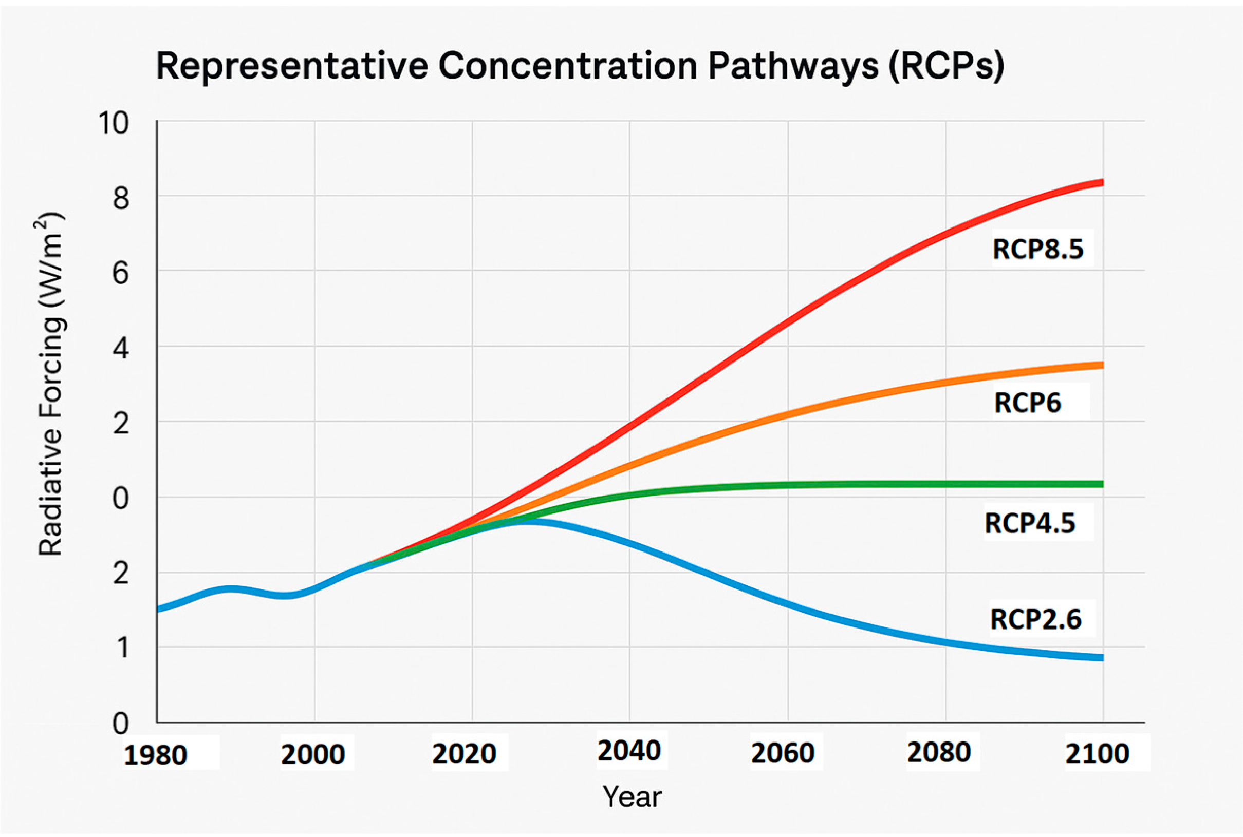
To assess the potential impacts of climate change on future air quality, it is essential to rely on high-resolution meteorological projections derived from regional climate models. These projections are based on greenhouse gas emission pathways, such as the Representative Concentration Pathways (RCPs), which describe different trajectories of radiative forcing levels by the end of the 21st century [32]. Among the most used scenarios are RCP4.5, representing an intermediate mitigation case, and RCP8.5, a high-emissions “business-as-usual” trajectory.

In this study, meteorological fields for future time horizons (2030 and 2050) are derived from the outputs of the CLIMAERA project (Interreg ALCOTRA Italia-Francia 2014–2020; https://www.climaera.eu, accessed on 22 August 2025). The regional simulations are performed using COSMO-CLM, the climate version of the non-hydrostatic COSMO-LM (Consortium for Small-scale Modeling—Limited-area Model), specifically adapted for long-term simulations of the Euro-Mediterranean region [33,34,35]. COSMO-CLM is widely used in the EURO-CORDEX initiative to provide dynamically downscaled climate projections at spatial resolutions of up to 0.11° (~12 km), which are particularly suitable for assessing climate impacts on regional air quality [10].

CLIMAERA adopted RCP4.5, which forecasts an increase in radiative forcing of 4.5 W/m² within 2100 (Figure 1). The scenario’s assumption is that the emission of CO₂ shall reduce under the actual levels within 2070, with an asymptotic emission around a doubling pre-industrial level within the end of the 21st century.

To simulate future air quality scenarios under changing climate conditions, meteorological projections derived from RCPs are used as input for chemical transport models (CTMs). This downscaling-coupling approach allows for the assessment of pollutant concentrations under consistent future climate and emission settings. In this study, meteorological outputs from the COSMO-CLM model were processed to drive the FARM, an Eulerian CTM widely applied in air quality studies across Italy [36] and Europe [37].

2.2. Modeling Framework and Coupling with CTM: FARM SMAL-LO

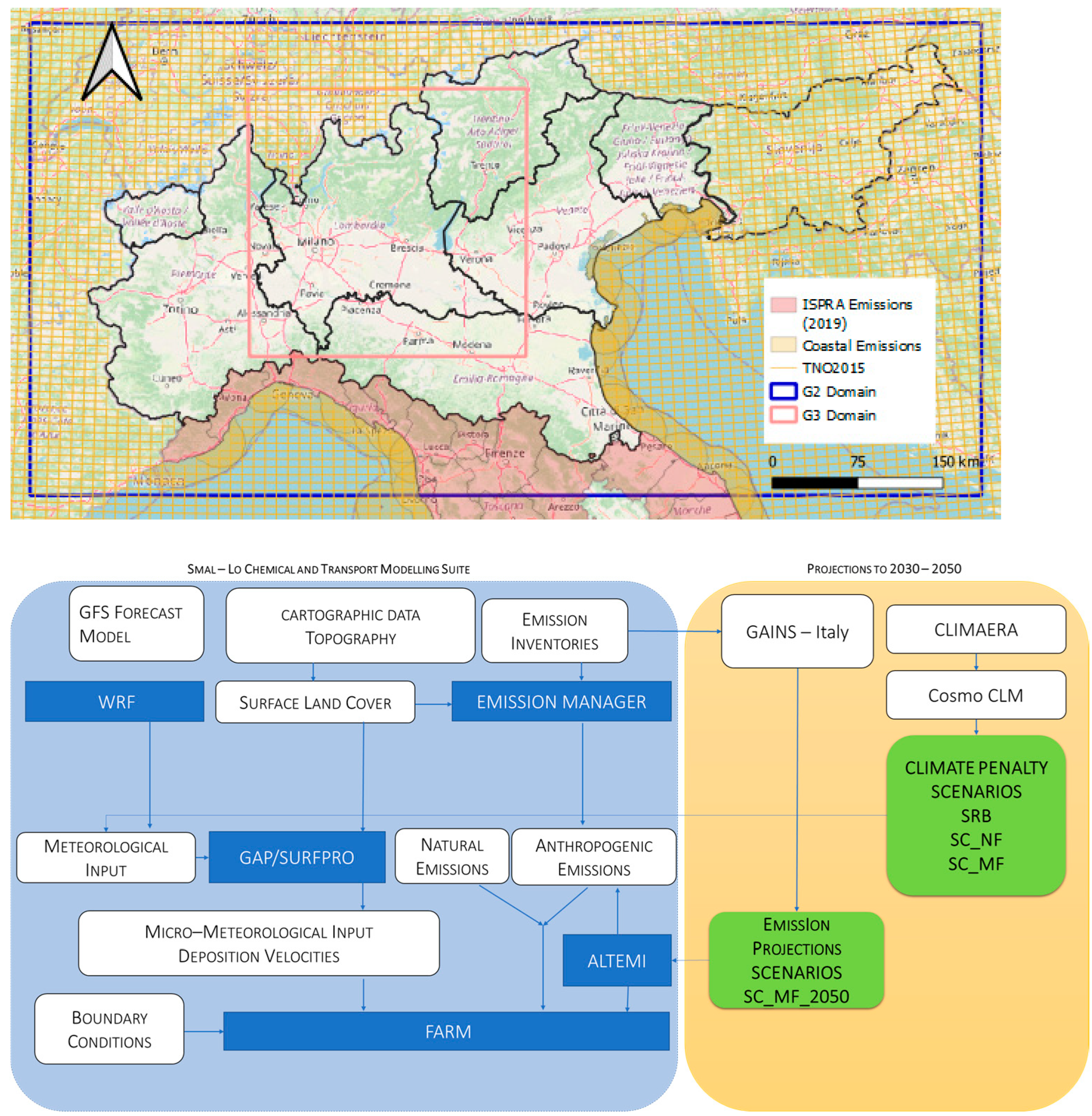
The air modeling system of ARPA Lombardia (SMAL-LO) is based on ARIA Regional developed by AriaNET srl and it is characterized by two different domain extension: one for the Lombardy Region (in Figure 2 represented by red line named g3) and one for the PREPAIR project (in Figure 2 represented by blue line named g2), which includes the Po Valley extended from the western (Piemonte and Valle d’Aosta Regions) to the eastern part (Slovenia) and from the northern (Trento Province and Friuli Venezia Giulia Region) to the southern part (Emilia-Romagna Region). The last one consists of 105 × 210 with a cell resolution of 4 km. The main workflow of modeling architecture is composed in Figure 2.

FARM simulates transport, deposition (wet and dry), and chemical transformation (droplet and gas-phase chemistry) of atmospheric pollutants with a full treatment of gas-phase and aerosol-phase chemistry using SAPRC-99 POPS-Hg [38], which includes 215 chemical reactions of more than 140 species. The aerosol module can aggregate species for aerosol concentrations, to have a comparison with measured data.

The coupling between COSMO-CLM and FARM is performed through a pre-processing chain that ensures consistency in meteorological fields, boundary conditions (QualeAria system, http://www.qualearia.it, accessed on 22 August 2025) and land-surface information, via WRF2FARM [39,40]. Emission inputs are provided through intermediate tool EMMA. It processes spatial (i.e., gridding on domain cells) and temporal (i.e., hourly) attribution of the inventory emission. For the LIFE PREPAIR Regions, the regional emission inventory of ARPA Lombardia, providing detailed emission data at the municipality level, was used [41]. In the initial phase of the study, emissions are held constrained to isolate the climate signal (i.e., the variability in pollutant concentrations driven solely by changes in meteorological conditions, rather than by changes emissions). This modeling approach enables the assessment of the so-called climate penalty on air quality [12], which refers to the potential degradation of air quality resulting from climate-induced changes in atmospheric dynamics.

No modifications were applied to the emission inventory to account for future socio-economic developments or technological advancements in this initial phase. Subsequently, an alternative simulation was conducted in which emissions were adjusted according to the Current Legislation scenario for Italy, to evaluate the system’s response to projected emission reductions by 2050.

2.3. “Climate Penalty” Scenarios

The reference year for meteorological conditions was 2015 with no emission variation to set up a climate penalty on air quality [12], as described in

Table 1. Definition of the “climate penalty” scenarios.

Name	Meteorology	Inventory
SRB	2015	2019–2021 constant
NF	2030	2019–2021 constant
MF	2050	2019–2021 constant
SC_MF_2050	2050	CLE 2050 projection

. The COSMO 2015 was used to simulate a Baseline Reference Scenario (named SRB), then by using a Near-Future (NF) meteorology extracted from the 5-year (2028–2032) COSMO-CLM and a Mid-Future (MF) meteorology extracted from the 5-year (2048–2052) COSMO-CLM. No data assimilation was performed for any of the scenarios considered.

In addition, an emission reduction scenario was run to see the effect of CLE with climate penalty quantification.

In the present study, the entire year is considered to compare the yearly thresholds indicated into the New EU Directive focusing on PM₁₀ and NO₂.

Furthermore, spatial distributions of relative percentage increase or decreases in pollutant concentrations, compared to the SRB, are presented for each grid cell across the Po Valley for all future scenarios. To do this, for each k-scenario, in correspondence to the j cell, the percentage variation Dj,k is computed as

$${\mathit{D}}_{\mathit{j},\mathit{k}}={\displaystyle \raisebox{1ex}{$\left({\mathit{C}}_{\mathit{b}\mathit{j}}-{\mathit{C}}_{\mathit{s}\mathit{j}\mathit{k}}\right)$}\!\left/ \!\raisebox{-1ex}{${\mathit{C}}_{\mathit{b}\mathit{j}}$}\right.}\ast 100$$

(1)

where ${\mathit{C}}_{\mathit{b}\mathit{j}}$ is the simulated concentration for the SRB and ${\mathit{C}}_{\mathit{s}\mathit{j}\mathit{k}}$ is the simulated concentration for the k-scenario.

2.4. Emissions and Emission Scenario

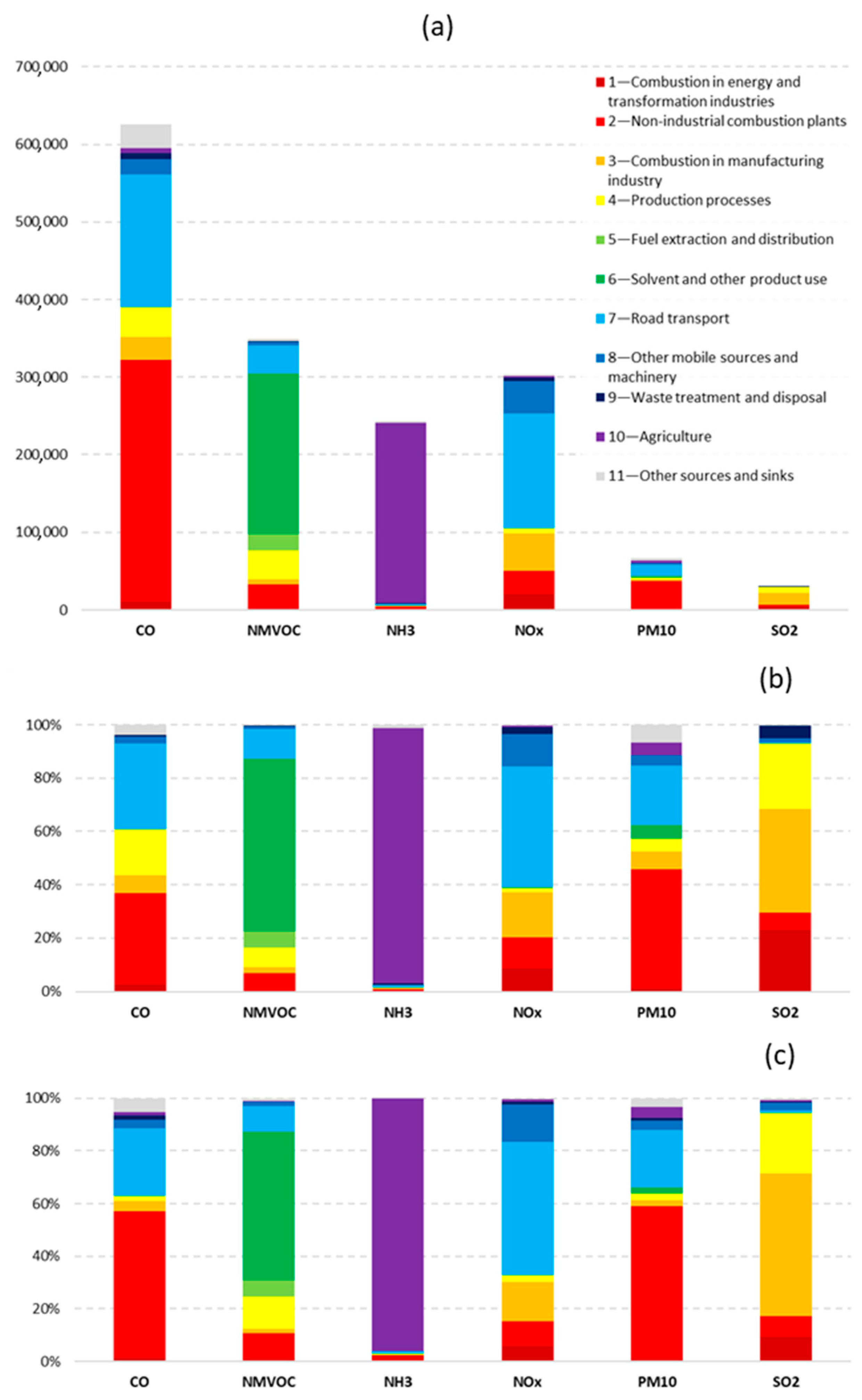
In this work, the emissions in the Po Valley are derived from the emission dataset provided by the project LIFE PREPAIR [41,42]. PREPAIR’s work has resulted in three updated emission inventories of PM_2.5, PM₁₀, TSP, NH₃, NO_x, SO₂, CO, and NMVOC for 2013, 2017, and 2019, based on data collected from the Environmental Protection Agencies and Regions of Lombardy, Emilia-Romagna, Piedmont, Veneto, Friuli Venezia Giulia, Valle d’Aosta, the Province of Bolzano, and the Province of Trento. The dataset provides high geographic resolution estimates at the municipal level using the SNAP source classification (Standard Nomenclature for Air Pollution). The emission input for the so-called “climate penalty” scenarios refer to 2019 for all the regions except for Lombardy where an update for 2021 has been introduced.

Figure 3 shows the total emissions for the domain and the contribution of the main macro sectors from the SNAP classification. Panel b and c clearly show as the main emission sources in Lombardy are very similar to those calculated for the other areas in northern Italy in the Po Valley. The comparability of emission sources supports the hypothesis in the first analysis of projecting Po Valley emissions into the future based on the forecasts obtained by the GAINS Italy system for Lombardy.

The GAINS model (Greenhouse Gas and Air Pollution Interactions and Synergies, https://iiasa.ac.at/, accessed on 22 August 2025), developed by the International Institute for Applied Systems Analysis (IIASA) throughout Europe and managed by ENEA for Italy, provides a reference system for the analysis of the costs and benefits related to different technological solutions, available to policy choices aimed at improving air quality and reducing greenhouse gas production. Emission scenarios can be obtained over a medium-term future time horizon, with five-year intervals.

The future emission trend provided by GAINS Italy is used to project the emission inventory to 2050 [43,44,45].

The emissions assessment obtained shows the expected trend of Lombardy’s emissions from 2021 in line with the scenario of the regulations in force in Italy and Lombardy (CLE). The evaluation involves hypotheses implemented by ENEA regarding the application of specific national and European policies concerning energy and industrial emissions and considers the technological evolution of already standardized systems, such as that of road vehicles, due to the progressive improvement of the circulating fleet.

In particular, the emission projections envisage the implementation of energy policies aimed at reducing the use of fossil fuels and energy consumption in homes. This development is already included in the evolution discussed here and will be implemented in the form of “existing legislation”, but it will have to be reflected in the actual implementation at national and local level.

In Figure 4, the total annual emissions foreseen for PM₁₀, NO_x, NH₃ and NMVOC show a progressive decrease compared to 2021. NO_x has the most consistent reduction while NMVOC and NH₃ have comparatively lower reductions. The projection analysis on single SNAP macro sector evidences the trend of specific source, which could not be relevant to the total amount of the emissions. NH₃ shows relative peaks in emissions in the period up to 2030 foreseen for on and off-road transport.

The resulting scenario represents the assessment of regional trend emissions on which further effects produced by the application of national and European legislation and the overall implementation of local air quality plans can possibly be inserted [46]. In any case, these forecasts are influenced by a series of factors, which, on the one hand, represent the main promoters of possible technological evolution. On the other hand, there are elements of possible uncertainties in the evaluations, including the following:

• Replacement of diesel cars: the renewal times of the circulating fleet control the speed with which emissions are reduced.
• Wear emissions: they represent the fraction of traffic emissions characterized by the least variation and directly linked to the demand for mobility.
• Use of natural gas in heating: the presence of biomass and gas heating systems determines a high degree of uncertainty linked to widespread habits and possible price fluctuations.
• Emissions of new wood-burning appliances: the effectiveness of the impact of Italian Ministerial Decree 186/2017 must be reflected in the definition of emission factors representative of the actual use of appliances in the future as well.
• Open fireplaces: the presence of these systems in homes is still documented in the project LIFE PREPAIR, their actual use, in addition to their number, represents a possible topic to be explored in the future as well.
• NH₃ emissions from livestock as shown: these are the ones that present the greatest difficulties in abatement.

2.5. Multivariate Statistical Analysis

Multivariate statistical techniques are particularly effective in environmental studies where each sample comprises multiple correlated hydro-chemical or atmospheric variables. In this study, multivariate analysis was used (1) to explore the relationships among simulated pollutants and meteorological variables and (2) to reduce the dimensionality of a complex dataset while preserving most of the original information. To this end, Principal Component Analysis (PCA) and Factor Analysis (FA) were employed.

PCA was applied to transform a set of interrelated observed variables into a new set of uncorrelated variables, known as principal components (PCs). These components are linear combinations of the original variables, with the first component capturing the maximum possible variance, and each successive component accounting for the next highest portion of remaining variance [47,48]. Although PCA efficiently reduces dimensionality, the interpretation of PCs can be challenging. Therefore, a Factor Analysis (FA) was subsequently performed to enhance interpretability by minimizing the influence of less significant parameters within each component.

The varimax rotation method [49] was applied to orthogonally rotate the factor loadings, thereby simplifying the structure and maximizing the sum of squared loadings for each factor. Factors with eigenvalues greater than 1 were retained and used as inputs for a subsequent Cluster Analysis (CA).

While PCA/FA identifies latent structures within the data, CA enables classification by grouping observations based on similarity. Specifically, the K-means clustering algorithm was applied to the varifactors derived from FA to distinguish spatial patterns of pollutant concentrations across monitoring stations. The clustering used Euclidean distance as the dissimilarity metric, grouping stations with similar contamination profiles—thus supporting the identification of similar patterns for each monitoring stations and locations [50].

All statistical analyses were performed using IBM SPSS Statistics (v28.0), while spatial mapping and distance calculations were carried out using QGIS (v3.16.5-Hannover).

3. Results

In this section, a description of the spatial and temporal variation in NO₂ and PM₁₀ concentrations with no emissions reduction is presented, and then modeled concentrations are compared against yearly thresholds of the New EU Ambient Air Quality Directive. Finally, statistical PCA/FA analyses were performed to find correlation between pollutants and some main meteorological parameters to better understand the link between climate change and air quality.

3.1. Maps and Comparison with New EU Ambient Air Quality Directive

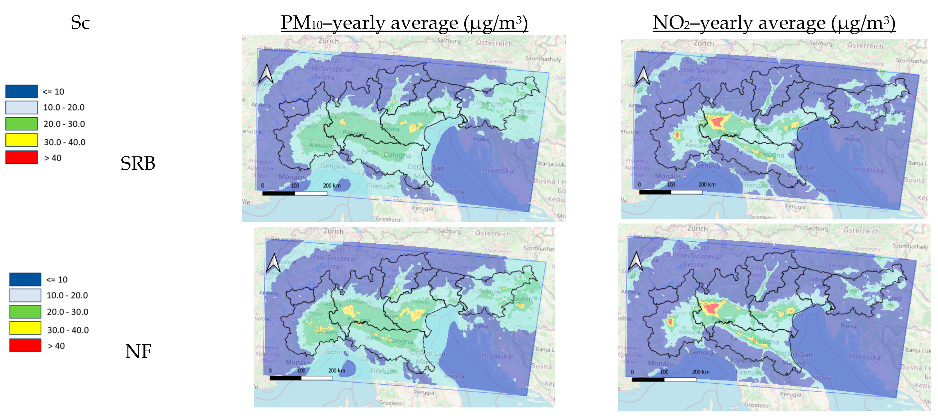
The results obtained from the annual simulations are presented as concentrations maps for each pollutant and scenario (Figure 5). In addition, both absolute and relative (percentage) differences were calculated between the SRB and the NF and/or MF scenarios.

For PM₁₀, under the SRB scenario, the highest concentrations were observed in the provinces of Milan and Lodi (Lombardy Region), in central Emilia-Romagna and in several areas of the Veneto Region. These values were significantly higher compared to those in the southern Apennines and northern Alpine arc. In the NF and MF scenarios, areas affected by elevated PM₁₀ concentrations expand to cover the entire Po Valley, including provinces such as Turin, Milan, Ferrara and Padua.

In terms of absolute differences, a reduction in PM₁₀ concentrations is mainly observed in mountainous regions (e.g., Trentino Alto-Adige, Aosta Valley and Friuli Venezia Giulia). However, in the lowland regions (e.g., Lombardy, Piedmont and Emilia- Romagna), the maximum concentrations in the MF scenario approach the limits set by Directive 2008/50/EC (as implemented in Italian Legislation by D.Lgs 155/2010). This indicates that climate change may exacerbate air pollution in already critical areas, making it more difficult to achieve the air quality standards set by the WHO guidance levels (15 μg/m³ for PM₁₀ and 10 μg/m³ for NO₂) and the New EU Ambient Air Quality Directive (Interim Target I.T.4 is 20 μg/m³ for PM₁₀ and 20 μg/m³ for NO₂)

In contrast, for NO₂, the SRB scenario reveals elevated concentrations in proximity to major urban centers and along primary road networks. No significant spatial changes in these critical areas are observed under the NF and MF scenarios. This is attributed to the fact that no emission reductions were included for NO₂ in the future simulations (MF and NF), underscoring the importance of including mitigation measures when assessing projected air quality (SC_MF_2050).

By using Equation (1), spatial distribution of relative percentage for each grid cell across Po Valley is computed and presented in Figure 6.

3.2. PCA/FA Outcomes

Since the emission reduction scenario is referred to 2050 projection, here, we presented the Principal Component/Factor Analyses and Cluster applied to only 2050. Details in 2030 are in Supplementary Materials (Figures S1 and S2, Table S1). PCA/FA was applied to 4 pollutants extracted from the MF scenario (NO₂, PM₁₀, PM_2.5, O₃) and some meteorological variables (Wind speed (WS), rainfall (prec), temperature (temp), pressure (pres), mixing height (hght), relative humidity (relh)) extracted by the COSMO-CLM fields.

PCA/FA initially extracted 4 rotated PCs, which accounted for about 75% of cumulative variance. To better interpret the components, the factor loadings matrix was rotated implementing the Varimax rotation criterion. The rotated factors loadings, being the correlation coefficients between each rotated PCs and each variable, are shown in

Table 2. Rotated Principal Component Matrix. Rotation Method: Varimax with Kaiser Normalization. Rotation converged in 7 iterations.

Rotated Component Matrix
Component Delta 2050–2015
	1	2	3	4
hght	−0.085	0.930	0.023	0.025
pres	0.094	0.175	−0.662	−0.180
Relh	0.127	−0.803	0.315	−0.049
Ws	−0.510	0.304	0.271	−0.119
Temp	0.112	0.907	−0.173	−0.011
Prec	−0.045	−0.112	0.756	−0.162
PM10	0.948	0.002	0.013	0.091
PM2.5	0.949	−0.003	0.011	0.097
NO2	0.788	0.032	−0.126	−0.269
O3	0.031	0.046	−0.007	0.959
Eigenvalue	2.82	2.62	1.084	0.981
% of Variance	28.27	26.73	10.84	9.80
Cumulative %	28.27	55.00	65.84	75.64

.

-

Varifactor 1: accounts for 28.3% of the variance and it is loaded mostly by PM₁₀, PM_2.5, NO₂ and Wind Speed (negatively);

-

Varifactor 2: accounts for 26.7% of the variance and it is loaded by temperature and mixing height and relative humidity (negatively);

-

Varifactor 3: accounts for 10.8% of the variance and it is loaded by rainfall and pressure (negatively);

-

Varifactor 4: accounts for 9.8% of the variance and it is loaded by Ozone.

Based on factor loadings, the extracted Factors can be interpreted as follows. In the first varifactor, three pollutants (PM₁₀, PM_2.5, NO₂) are heavily correlated compared to the other varifactors and there is a negative correlation with Wind Speed. The second and third varifactors contained only meteorological variables suggesting that there is no direct correlation with pollutants for these meteo-conditions (i.e., if wind speed increases relative humidity decreases and the mixing height could increase).

The fourth varifactor included two pollutants: one positively correlated with the varifactor (O₃), and one negatively correlated (NO₂). This occurs when two or more pollutants are negatively correlated but their variation is independent with respect to the other variables used in PCA/FA.

The PCA/FA results highlight key meteorological drivers influencing pollutant variability, with wind speed and precipitation emerging as the main factors. These statistical findings closely match the CTM simulations, where decreases in wind speed and precipitation lead to increased PM₁₀ and NO₂ concentrations under the NF and MF scenarios.

3.3. CA Outcomes

K-means cluster analysis was applied on the extracted varifactors from the Factor Analysis (FA). After several trials, the number of clusters (K) was set to 5, resulting in five distinct clusters derived from the varifactors. The clustering procedure was run twice to ensure stability: the first run identified initial centroids, which were then used after as starting points in the second run to achieve convergence and more stable cluster assignments.

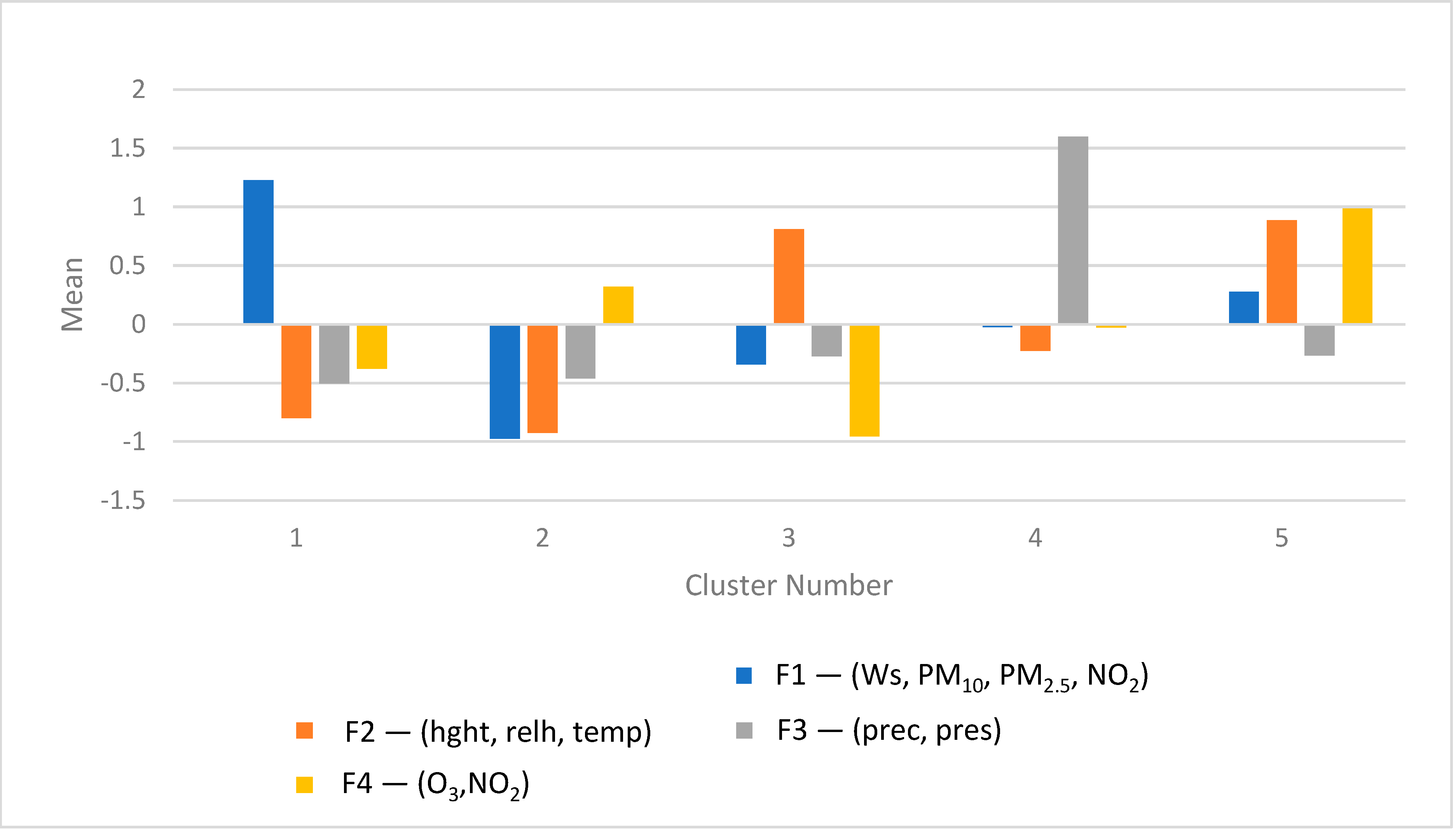
Figure 7 shows the deviation of each cluster’s mean varifactor values from the overall dataset mean. Longer bars indicate stronger deviations from the mean (set at zero), highlighting variables with high discriminative power within each cluster. For example, Cluster 1 is characterized by elevated concentrations (e.g., 1–2 times above the mean) of pollutant-related factors. In contrast, Cluster 2, dominated by the first principal component (PC1), exhibits concentration values approximately one standard unit below the mean.

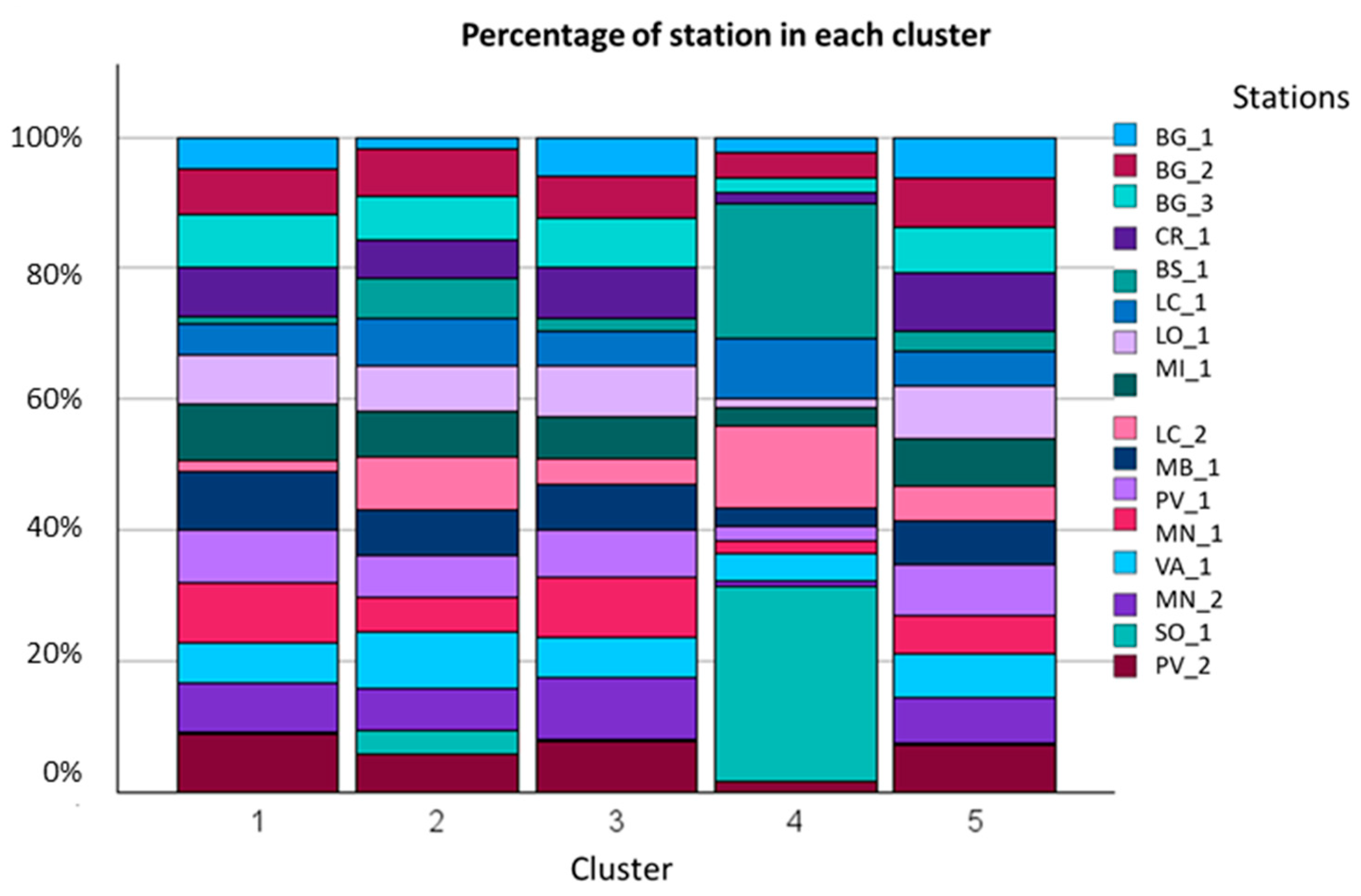
Still, referring to Figure 8 and focusing on the Lombardy Region, the number of observations representing each monitoring station within each cluster is also shown. Cluster Analysis (CA) enables the identification of the most “representative” station (s) for each cluster. For instance, BS_1 and SO_1 stations—located in mountainous areas—are predominantly associated with Cluster 4, which shows higher values of Factor 3 (F3), typically linked to increased precipitation and lower pollutant concentrations (Figure 8). Conversely, these stations are absent from Cluster 1, which is characterized by high pollutant levels and reduced wind speed conditions typical of the central Po Valley.

Cluster Analysis groups stations with similar meteorological–pollutant patterns, distinguishing urban/lowland areas (Clusters 1 and 5) from mountainous/ventilated areas (Cluster 4). These typologies align spatially with the identified climate penalty zones, confirming the role of local meteorology in shaping projected pollutant levels.

The same analysis was performed for the NF scenario, and the corresponding figures are provided in the Supplementary Materials.

Mapping stations with cluster belonging (Figure 9) we can see that mountainous stations do not change their cluster number (4) from 2030 to 2050, remaining affected only by meteorological parameters. On the other hand, on the Pre-Alps and Plain, some stations change their prevalent cluster behavior from 2030 to 2050 (i.e., passing from only meteo-dependency (Cluster 2 2030) to only contaminants dependency (Cluster 5 2050)). This should be investigated for possible chemical regime change during climate change events.

4. Discussion

Emission projections to 2050 are influenced by various technical assumptions as well as by the degree of implementation of current legislation and policy measures. Under these scenarios, emissions are expected to progressively decrease over time. However, in the long term, climate variation may significantly alter atmospheric dispersion characteristics and the chemical reactivity of pollutants, introducing an additional source of uncertainty.

In this study, we attempted to quantify the potential impact of climate change on pollutant dispersion by introducing so-called “climate penalty” scenarios in which emissions are held constant while meteorology fields vary. This approach allows us to explore how climate- induced changes could undermine the expected improvements in air quality resulting from emission reductions aligned with Current Legislation in Italy (Figure 4) by 2050.

The “climate penalty” scenarios indicated a general increase in PM₁₀ and NO₂ concentrations in both 2030 and 2050 compared to SRB. Moreover, through Factor Analysis (FA) and Principal Component Analysis (PCA), we explored the relationships between variations in pollutant concentrations and key meteorological parameters. The integration of PCA/FA and CTM results provides a mechanistic understanding of the climate penalty: statistical analysis identifies the meteorological variables driving pollutant increases, while the transport model quantifies their spatial and temporal impacts. The results suggest that increases in PM₁₀ and NO₂ concentrations are strongly associated with projected decreases in wind speed, implying more frequent stagnant conditions and thus exacerbating the problem of air pollution in the Po Valley.

When evaluating the SC_MF_2050 scenario, which combines 2050 meteorology with emissions projected under Current Legislation, we observe a general reduction in concentrations. However, it is essential to assess this “beneficial” scenario in the context of the new EU Ambient Air Quality Directive which sets more stringent targets than current standards (Interim Target I.T.4 is 20 μg/m³ for PM₁₀ and 20 μg/m³ for NO₂ whereas under D.lgs 155/2010 are both 40 μg/m³).

By comparing the absolute differences between the MF (climate-only) and SC_MF_2050, (climate plus mitigation) scenarios, we identified the so-called climate penalty zone for the main contaminants. These are areas (Figure 10) where the projected increase in concentration due to climate change (MF) exceeds the benefit obtained from emission reduction scenario (SC_MF_2050). For NO₂, the “climate penalty zone” are predominantly aligned with major roads networks, while for PM₁₀ (and PM_2.5), they are mostly located across the central lowlands, confirming the findings of the cluster analysis. Furthermore, for O_3, when considering 93.15yh percentile maximum daily 8 h average concentration, negative areas extend over the entire Po Valley, except for the main road corridor in Emilia-Romagna. These results are consistent with the PCA/FA outcomes, where ozone appears only in Factor 4 (Table 2).

Similar patterns are observed when considering RID (mitigation) and different meteorological input (SRB and MF meteo), confirming that future mitigation strategies could be undermined by climate change (Supplementary Materials—Figure S3). Specifically, Cluster 4, characterized by higher precipitation, lower temperature and stable pollutant levels, is primarily located in mountainous areas. In contrast, Clusters 1 and 5, associated with increased concentrations, higher temperature and lower precipitation, are found in more urbanized areas and along major roads. This approach highlights that future air quality deterioration is primarily driven by increased stagnation, detected both statistically and in the simulated concentrations, particularly in urbanized lowland areas.

An additional layer of complexity arises from the indirect interactions between climate parameters (e.g., temperatures) and socio-economic system. These effects are typically not included in emission projection models, yet they may substantially influence key emissions drivers such as energy consumption for heating and cooling, animal production for meat and milk, cultivation yields and urban planning.

5. Conclusions

This study investigated the potential impacts of climate change on air quality in the Po Valley, a region already subject to chronic exceedances of pollutant thresholds due to its orographic configuration, high population density, and industrial activity. By integrating regional climate projections with chemical transport modeling under different meteorological scenarios (SRB, NF, MF), and isolating the influence of climate while keeping emissions constant, we quantified the so-called climate penalty—i.e., the adverse effects of climate-driven meteorological changes on pollutant concentrations, independent of emission trends.

The results indicate that, despite expected emission reductions under the Current Legislation, climate change could partially offset these benefits by increasing the frequency of stagnant atmospheric conditions and reducing pollutant dispersion, particularly in lowland urbanized areas. Notably, increases in PM₁₀ (the same behavior is observed in PM_2.5) and NO₂ concentrations in 2030 and 2050 were closely associated with decreasing wind speed and precipitation, as shown by multivariate statistical analyses (FA/PCA and cluster analysis). The identification of climate penalty zones, where the increase in pollution due to climate change outweighs the gains from mitigation, highlights critical areas—especially along major roads and in the central plain—where additional measures may be required. Considering 93.15th percentile O₃, we can see that the penalty areas extend over the entire Po Valley (unlike PM and NO₂, as also highlighted in the PCA, where O₃ appears separately in F4), offsetting the potential benefits of emission reductions under Current Legislation.

These findings underscore the importance of integrating climate resilience into air quality planning. While emission reduction remains essential, future policies should also account for the evolving climatic context, especially in regions like the Po Valley where atmospheric conditions are highly sensitive to climate variability. Moreover, the indirect effects of climate change on socio-economic drivers—such as energy demand, agricultural practices, and urban development—must be considered in long-term emission projections to avoid underestimating future challenges. Considering the upcoming EU Ambient Air Quality Directive, which sets more stringent targets in alignment with WHO guidelines, comprehensive and adaptive strategies will be necessary to ensure air quality improvements under changing climate.