Transitions of Carbon Dioxide Emissions in China: K-Means Clustering and Discrete Endogenous Markov Chain Approach

Abstract

This study employs k-means clustering to group 30 Chinese provinces into four CO₂ emission patterns, characterized by increasing emission levels and distinct energy consumption structures, and captures their dynamic evolution from 2000 to 2021 using a discrete endogenous Markov chain approach. While Shanghai, Jiangxi, and Hebei retained their original classifications, provinces such as Beijing, Fujian, Tianjin, and Anhui transitioned from higher to lower emission patterns, indicating notable reversals in emission trajectories. To identify the determinants of these transitions, GDP growth rate, population growth rate, and energy investment are incorporated as time varying covariates. The empirical findings demonstrate that GDP growth substantially increases interpattern mobility, thereby weakening state persistence, whereas population growth and energy investment tend to reinforce emission pattern stability. These results imply that policy responses must be tailored to regional dynamics. In rapidly growing regions, fiscal incentives and technological upgrading may facilitate downward transitions in emission states, whereas in provinces where emissions remain persistent due to demographic or investment related rigidity, structural adjustments and long term mitigation frameworks are essential. The study underscores the importance of integrating economic, demographic, and investment characteristics into carbon reduction strategies through a region specific and data informed approach.

1. Introduction

Climate change has emerged as an acute global challenge in recent years, precipitated by accelerated industrialization and urbanization that have substantially amplified greenhouse gas emissions, most notably carbon dioxide (CO₂). As highlighted by Li [1], Kocak and Alnour [2] and Kao et al. [3], China’s heavy reliance on coal and fossil fuels for power generation has made it the world’s largest emitter of CO₂. According to the International Energy Agency [4], China accounted for roughly 35% of global CO₂ emissions in 2023. The nation’s sustained economic expansion, coupled with escalating energy consumption, particularly in the electricity sector, has further exacerbated CO₂ emissions [5]. Although China has achieved notable progress in energy conservation and efficiency improvement, its emissions remain substantially higher than other developed nations [6]. Therefore, enhancing energy infrastructure investment, accelerating energy efficiency innovations, and restructuring industrial composition are of great importance to meet emission reduction objectives [6,7]. Gui et al. [8] advocated for dynamic monitoring of the spatiotemporal evolution of carbon emissions to enable precision mitigation strategies.

In light of the imperative for targeted carbon mitigation, this study aims to deliver a comprehensive understanding of provincial carbon emission dynamics and inform the design of region-specific mitigation strategies. To achieve this aim, we pursue three key objectives. First, we deploy k-means clustering to classify multi energy CO₂ emission series from 30 Chinese provinces from 2000 to 2021 into four patterns and chart their initial transition trajectories. Second, to address clustering’s inability to capture causal mechanisms of pattern evolution, we integrate GDP growth, population growth, and energy investment as time-varying covariates into a discrete endogenous Markov chain framework. Third, we apply this composite model to estimate how these socioeconomic covariates modulate transition probabilities among emission states.

Methodologically, this study utilizes k-means clustering, a prevalent unsupervised learning technique, to cluster provinces for each time period according to their carbon emission profiles. The method partitions observations into homogeneous clusters, maximizing intra-cluster homogeneity and inter-cluster heterogeneity [9,10]. He et al. [11] and Dong et al. [12] underscored its algorithmic simplicity, computational tractability, and scalability to high-dimensional datasets. Liu et al. [13] and Dong et al. [12] illustrated its capacity to resolve latent structural heterogeneity across provincial emission trajectories, thereby mitigating subjective classification biases and ensuring classification robustness.

The Markov chain is a probabilistic model that formalizes the likelihood of state transitions over time. Given the heterogeneous characteristics of distinct clusters, understanding their temporal evolution is crucial from an environmental policy standpoint. The Markov framework aptly captures the stochastic dynamics of emission-pattern transitions and has therefore been extensively employed to examine shifts in carbon emission states [14,15]. Moreover, Chen and Wu [16] and Huang et al. [17] emphasize its proficiency in modeling the intrinsic probabilistic behavior of environmental monitoring data. In this study, we adopt a discrete endogenous Markov chain model to investigate the determinants of these transitions, as exemplified by Putter et al. [18] and Yuan et al. [19], who demonstrate its capacity to capture continuous-time state shifts, incorporate time-varying covariates, and accommodate unobserved heterogeneity in panel contexts. Building on this modeling paradigm, we integrate GDP growth rate, population growth rate, and energy investment into an aggregated covariate index (ACI) to systematically evaluate their influence on transitions among carbon emission patterns.

To place these empirical insights in context, we next contrast our comprehensive, covariate-driven Markov framework with existing clustering and modeling approaches in the literature. Previous studies have utilized hierarchical clustering [20,21]. However, these studies were often restricted to single sectors (e.g., electricity) and shorter time frames [11,22,23] or focused on limited emission indicators such as industrial energy efficiency or cumulative emissions [12,13]. In contrast, this study employs comprehensive, multi-energy CO₂ emission data covering 30 provinces from 2000 to 2021. This study combines k-means clustering with discrete Markov chain modeling, incorporates GDP growth, population growth and energy investment as covariates, and builds transition matrices at their 0.25, 0.5 and 0.75 quantiles to reveal effects on emission state dynamics and stability.

The remainder of this paper is structured as follows: Section 2 reviews the relevant literature; Section 3 describes the data sources; Section 4 examines K-means clustering and discrete endogenous Markov chain models; Section 5 presents the empirical findings based on these models; and Section 6 is the conclusion of our study.

2. Literature Review

2.1. K-Means Clustering Analysis Method

Cluster analysis is a classical unsupervised machine learning approach, with k-means clustering widely applied for classifying and identifying patterns in multivariate datasets [24]. Within the field of carbon emissions research, clustering methods are extensively utilized to categorize emission patterns across different countries and regions, thereby facilitating policymakers in formulating targeted emission-reduction strategies. Kijewska and Bluszcz [25] used k-means clustering to classify European countries based on greenhouse gas emissions, clearly illustrating differences in national emission patterns and informing EU-level climate policies. Jimenezpreciado et al. [10] applied k-means clustering to identify distinct CO₂ emission patterns across 208 countries, enabling comparisons between emissions and economic development stages. These studies demonstrate the effectiveness and broad applicability of k-means clustering in carbon emissions research, providing valuable empirical insights for regional emission analyses in China.

In the context of China, clustering methods have become increasingly prominent analytical tools for examining regional carbon emission patterns. Wang and Yu [9] employed a k-means clustering method to classify 30 Chinese provinces into four distinct emission categories using provincial-level CO₂ data from 2000 to 2018. A notable contribution of Wang and Yu [9] is their dynamic approach to studying emission pattern transitions over time, addressing a limitation of prior research that often remained confined to static classifications. However, their analysis had limitations. Although they documented emission pattern transitions, they did not investigate how socioeconomic factors influence these transitions, thus limiting policy implications. In this study, we not only adopt the effective clustering approach of Wang and Yu [9] but also expand it by exploring the impacts of GDP growth rate, population growth rate, and energy investment on emission-pattern transitions, thereby addressing previously unexplored mechanisms underlying emission dynamics.

Several other studies have also employed clustering methods to analyze regional carbon emissions. He et al. [11] and Wang et al. [23] utilized K-means clustering to assess the CO₂ reduction potential within provincial electricity sectors. Hu et al. [22] applied K-means clustering to identify provinces with significant reductions in emissions during the COVID-19 pandemic. Although these studies confirm the advantages of clustering methods for policy design, they share limitations: narrow data scopes, sector-specific focus (e.g., electricity), short time frames, and lack of dynamic analyses.

2.2. Discrete Endogenous Markov Chain Model

Discrete endogenous Markov chain frameworks extend conventional Markov processes by permitting transition probabilities to vary with observed covariates and to exhibit correlations with disturbance terms. In their seminal contribution, Kim et al. [26] introduced a bivalent regime specification that embeds a Gaussian Probit mechanism for regime switching, jointly estimating the regime shock covariance via a modified Hamilton filter and assessing exogeneity through a likelihood ratio test. Building on this foundation, Hwu et al. [27] proposed a multinomial Probit formulation accommodating an arbitrary number of states, imposed a multivariate Gaussian covariance structure among regime disturbances, and deployed an iterative filtering algorithm that maintains computational tractability while ensuring reliable finite sample performance. Peng et al. [28] further adapted the discrete endogenous paradigm to a continuous time context under partial information, integrating Wonham filtering with an extended Hamilton–Jacobi–Bellman framework to derive time-consistent strategies in hidden Markov markets. These sophisticated methodologies have also demonstrated efficacy in characterizing carbon emission dynamics at both global and regional scales. For example, Huang et al. [17] employed kernel density estimation alongside Markov chains to investigate CO₂ emission intensity dynamics and convergence across 92 countries from 1999 to 2021, thereby elucidating policy implications for high and low emission nations.

Accordingly, the present study adopts a discrete endogenous Markov chain framework to elucidate the drivers of emission state transitions, thereby enhancing the precision of transition probability estimation and reinforcing the policy salience of its insights. Unlike conventional applications that emphasize output volatility or financial regime classification, this study pioneers the application of the framework to province level CO₂ emission clusters in China, which are identified via k-means clustering techniques. By permitting transition intensities to vary flexibly with time varying covariates, the model captures the evolving influence of macroeconomic and demographic conditions on inter pattern mobility. Furthermore, through the differentiation between persistent and transitional emission states and the quantification of covariate impacts on these dynamics, the model enhances analytical transparency and facilitates the development of more regionally tailored mitigation strategies.

2.3. Variable Selection

CO₂ emission transitions are modeled as functions of economic growth, demographic dynamics and infrastructure investment. Accordingly, GDP growth rate, population growth rate, and energy investment are included as covariates. The discrete endogenous Markov chain framework then reveals how these factors drive provincial emission state dynamics.

Azevedo, Sartori, and Campos [29] identified GDP growth as a primary driver of CO₂ emissions among BRICS countries, and Marjanović, Milovančević, and Mladenović [30] similarly linked economic expansion to rising emissions. Based on these findings, this study incorporates GDP growth as a covariate. Population growth emerges as another significant factor. Wang, Kang, and Xu [31] documented a positive association between provincial population size and CO₂ emissions in China, while Shaari, Abidin, and Ridzuan [32] emphasized how population increases in developing regions amplify energy demand and emissions, and Yu, Deng, and Chen [33] examined the impact of population aging on consumption patterns. Thus, population growth rate is included as an explanatory variable. Finally, energy investment influences emissions: Li and Li [34] employed spatial econometric models to show that infrastructure investments elevate emissions alongside growth, and Kuang, Akmal, and Li [35] noted that despite green technology advances, coal remains the dominant energy source in China. Therefore, energy investment is added as a covariate to clarify its effect on emission-pattern transitions. The integration of GDP growth, population growth, and energy investment supports a unified evaluation of their combined impact on emission pattern dynamics.

3. Methodology

3.1. K-Means Clustering Analysis

K-means clustering is employed to classify complex, multidimensional carbon emission datasets by grouping observations with similar characteristics; He et al. [11] demonstrated its ability to reveal structural differences in provincial emission profiles and Kijewska and Bluszcz [25] showed that it achieves high classification accuracy to inform targeted emission reduction policies. Based on these advantages, this study adopts k-means clustering as its primary analytical approach.

To measure within-cluster compactness and minimize the dissimilarity among observations in the same cluster, this study adopts the within-cluster sum of squares (WSS) as the optimization criterion for k-means clustering. Let the CO₂ emission data set $X=\{x_1,\dots ,x_n\}$ comprise all provincial emission values across years or energy categories. k-means partitions X into k disjoint clusters $S=\{S_1,\dots ,S_k\}$ and selects the partition that minimizes

$$arg\underset{S}{min}\sum _{i=1}^k\sum _{x\in S_i}{∥x-{\mu }_i∥}^2,$$

(1)

where ${\mu }_i$ denotes the centroid of cluster i, representing the central level of that emission pattern. The objective of k-means clustering is to identify a set of clusters that minimizes the sum of squared errors between provincial emission characteristics and their respective cluster centers, thus effectively characterizing typical provincial carbon emission patterns.

Because no analytical solution exists for the global objective in Equation (1), the algorithm proceeds by alternating two steps until assignments or centroids stabilize. The first step is the assignment step, which allocates each data point (carbon emission characteristic for each province) to the cluster whose centroid has the minimum squared Euclidean distance. Formally, this can be written as

$$S_i^{\left(t\right)}=\left\{x_j:{\parallel x_j-{\mu }_i^{\left(t\right)}\parallel }^2\le {\parallel x_j-{\mu }_m^{\left(t\right)}\parallel }^2,\forall m\in \{1,\dots ,k\}\right\},$$

(2)

which serves to identify the set of observations belonging to cluster i at iteration t. In Equation (2), $S_i^{\left(t\right)}$ denotes the set of observations assigned to cluster i at iteration t; $x_j$ is the feature vector of province j; ${\mu }_i^{\left(t\right)}$ and ${\mu }_m^{\left(t\right)}$ denote the centroids of clusters i and m at iteration t.

The second step is the centroid update step, in which the centroid of each cluster is recalculated as the mean of all points currently assigned to that cluster. This is given by

$${\mu }_i^{(t+1)}={\displaystyle \frac{1}{\left|S_i^{\left(t\right)}\right|}}\sum _{x_j\in S_i^{\left(t\right)}}{x}_j.$$

(3)

Equations (2) and (3) define the iterative assignment and centroid update procedures, which jointly minimize the global optimization objective specified in Equation (1). The use of the arithmetic mean to determine cluster centers offers significant advantages for emission data exhibiting gradual variation rather than abrupt regime shifts. In this study, provinces are classified based on annual CO₂ emissions and energy composition, which are characterized by monotonic increases in total emissions along with discrete structural shifts in energy use across clusters. The arithmetic mean provides a stable and interpretable representation of each cluster by aggregating all assigned observations, thereby mitigating the influence of short-term fluctuations or local outliers. As shown in Equation (3), this averaging process ensures that the resulting centroids minimize within cluster variance under the WSS criterion, which serves as a transparent and quantitative metric of cluster compactness. This property is particularly suitable for carbon emission data, where interprovincial variation is continuous and multidimensional.

By standardizing all observations and applying k-means clustering independently to each year, the study ensures both cross-sectional comparability and temporal consistency. The mean-based clustering mechanism contributes not only to the statistical robustness of the findings but also enhances their interpretability in the context of policy oriented analysis.

3.2. Optimal Number of Clusters

To determine the optimal number of clusters k for the k-means algorithm, we utilize the Elbow Criterion predicated on WSS as specified in Equation (1). While WSS diminishes with increasing k, its marginal decrease becomes insubstantial beyond a threshold. Plotting WSS versus successive k values reveals an elbow point where the curve begins to plateau, denoting the optimal balance between model parsimony and explanatory fidelity.

To augment this visual assessment, we introduce the D-index as a quantitative measure of clustering cohesion gains with respect to k. We calculate both the first-order and second-order differences of the D-index, selecting the k at which these metrics exhibit a marked decline followed by plateauing. Convergence of both the Elbow Criterion and the D-index equips us with a rigorous, reproducible determination of the optimal k.

3.3. Markov Chain Model

This study employs a continuous-time multi-state Markov model to characterize the dynamic transitions of carbon emission patterns for 30 Chinese provinces over the study period. Suppose province m occupies state r at time t. The transition from state r to state s within the state space $\{1,2,3,4\}$ is governed by the transition intensities $q_{rs}(t;z\left(t\right))$, which denotes the instantaneous rate of moving from state r to state s conditional on covariates $z\left(t\right)$. These instantaneous rates $q_{rs}(t;z\left(t\right))$ collectively form the $4\times 4$ transition intensity matrix Q:

$$Q=\left[q_{rs}(t;z\left(t\right))\right],$$

(4)

whose off-diagonal entries are defined as follows:

$$q_{rs}(t;z\left(t\right))=\underset{\Delta t\to 0}{lim}{\displaystyle \frac{Pr\left[X(t+\Delta t)=s\left|X\right(t)=r\right]}{\Delta t}},r\ne s,$$

(5)

where $X\left(t\right)$ denotes the emission state occupied by a province at time t. To ensure that each row of Q sums to zero, the diagonal entries are defined by

$$q_{rr}(t;z\left(t\right))=-\sum _{s\ne r}{q}_{rs}(t;z\left(t\right)).$$

(6)

In this study, matrix Q specifically denotes the instantaneous transition intensities among states, representing the rate at which transitions occur within an infinitesimal time interval.

Let $t=\left(t_{m1},t_{m2},\dots ,t_{mh}\right)$. Markov chain models applied to panel data typically assume the Markov property, meaning that future states depend exclusively on the current state and are independent of history. Under this assumption, the transition probability matrix $P(u,t+u)$ of the multi-state model can be defined and computed using the Kolmogorov differential equations. Specifically, when the transition intensity matrix Q remains constant over the time interval $(u,t+u)$, the relationship between the transition probability matrix $P(u,t+u)$ and the matrix Q is given by

$$P(u,t+u)=P\left(t\right)=exp\left(tQ\right),$$

(7)

where $exp\left(tQ\right)$ denotes the matrix exponential function, representing the relationship between the transition probability matrix $P\left(t\right)$ and the transition intensity matrix Q.

To estimate the transition intensity matrix Q within the Markov chain model, this study applies maximum likelihood estimation (MLE). The overall likelihood function can be expressed as the product of the state transition probabilities for each province m and each observation interval h. The estimation equation is expressed as follows:

$$L\left(Q\right)=\prod _{m,h}{p}_{S\left(t_{mh}\right),S\left(t_{m,h+1}\right)}\left(t_{m,h+1}-t_{mh}\right),$$

(8)

where $m=\{1,2,\dots ,30\}$ indexes the thirty provinces, and $h=\{1,2,\dots ,22\}$ indexes the annual observation periods from 2000 through 2021 for each province. Here, $t_{mh}$ denotes the time at which province m is observed in period h. The term $p_{S\left(t_{mh}\right),S\left(t_{m,h+1}\right)}\left(t_{m,h+1}-t_{mh}\right)$ denotes the probability of province m transitioning from the state observed at time $t_{mh}$ to the state observed at the subsequent time $t_{mh+1}$. By maximizing this likelihood function, one obtains the maximum likelihood estimate of the transition intensity matrix Q.

To address the research objectives, this study incorporates GDP growth rate, population growth rate, and energy investment as covariates into the Markov model. The covariates are included using a proportional intensity model, thereby adjusting the transition intensities $q_{rs}(t;z\left(t\right))$ as follows:

$$q_{rs}\left(t;z\left(t\right)\right)=q_{rs}^{\left(0\right)}\left(t\right)exp\left({\beta }_{rs}^{T}z\left(t\right)\right),$$

(9)

where $q_{rs}(t;z\left(t\right))$ is the covariate-adjusted instantaneous transition intensity from state r to state s at time t. The baseline intensity $q_{rs}^{\left(0\right)}\left(t\right)$ corresponds to the transition intensity without covariates. The term ${\beta }_{rs}^T$ denotes the vector of regression coefficients associated with the covariate vector $z\left(t\right)$, reflecting the magnitude and direction of each covariate’s effect. The covariate vector $z\left(t\right)$ collectively represents the standardized values of GDP growth rate, population growth rate, and energy investment at time t.

Having detailed the theoretical framework and methodological specifications of both k-means clustering and the discrete endogenous Markov chain approach, this study now presents empirical results. These results reveal carbon emission patterns and their dynamic transition paths identified via k-means clustering and further investigate how covariates influence transitions among emission patterns through the discrete endogenous Markov chain approach.

4. Data Description and Processing

The carbon dioxide emission data employed in this study are obtained from the Carbon Emission Accounts and Datasets (CEADs), covering the period 2000 to 2021 for 30 provinces, municipalities and autonomous regions in China. CEADs provides detailed provincial-level emissions data across major energy sources, including coal, petroleum, and natural gas. Additionally, data on GDP growth rates, population growth rates, and energy investment were collected from the National Bureau of Statistics of China (NBSC).

Table 1. Summary of descriptive statistics for key covariates.

Covariate	Mean	S.D.	Min	Max
GDP Growth Rate	0.1260	0.0589	−0.0534	0.2981
Population Growth Rate	0.0066	0.0121	−0.0555	0.0578
Energy Investment (billion CNY)	562.5599	548.5029	6.5800	3382.5100

reports the descriptive statistics of the key covariates incorporated in the analysis, detailing their respective means, standard deviations, and ranges.

Table 2. Descriptive statistics of variables (unit: million tonnes).

Sources of CO2 Emissions	Mean	S.D.	Min	Max
Total	260.5944	199.4786	0.8144	947.1629
Raw Coal	146.8090	117.0447	<0.0001	677.8168
Cleaned Coal	2.4558	4.8659	<0.0001	44.7477
Other Washed Coal	4.5788	7.4144	<0.0001	53.9283
Briquettes	2.9229	5.0609	<0.0001	34.9681
Coke	29.5269	40.0912	<0.0001	276.3979
Coke Oven Gas	2.8430	3.9087	<0.0001	23.8529
Other Gas	12.3505	23.6712	<0.0001	227.3464
Other Coking Products	0.9034	1.7830	<0.0001	18.8365
Crude Oil	0.8220	1.9771	<0.0001	17.4008
Gasoline	9.5943	8.1804	<0.0001	45.6461
Kerosene	2.0671	3.3964	<0.0001	22.8694
Diesel Oil	14.4089	10.5344	<0.0001	56.1323
Fuel Oil	3.3378	6.3668	<0.0001	50.2534
LPG	2.5162	3.6811	<0.0001	23.1204
Refinery Gas	1.5249	1.8210	<0.0001	13.1969
Other Petroleum Products	0.2878	0.6784	<0.0001	7.9293
Natural Gas	8.8971	10.3553	<0.0001	62.3759
Process	14.7480	14.3752	<0.0001	56.6568

Note: The minimum values are reported to four decimal places to accurately reflect the observed minima.

presents descriptive statistics of CO₂ emissions by energy source for 660 province-year observations in 30 Chinese provinces from 2000 to 2021, reporting the number of observations, mean, standard deviation, minimum and maximum values. In this table, the term of “Total” refers to the sum of CO₂ emissions from all listed energy sources for each province–year. Overall, total emissions average 260.59 million tonnes with a standard deviation of 199.48 million tonnes, ranging from 0.81 to 947.16 million tonnes and reflecting substantial inter-provincial heterogeneity. Raw coal emissions average 146.81 million tonnes and reach a maximum of 677.82 million tonnes; other fuels (e.g., petroleum, natural gas) exhibit similarly wide distributions. This pronounced cross-provincial and temporal variation in emission volumes provides the empirical foundation for the subsequent k-means clustering analysis of emission patterns.

5. Empirical Results

5.1. Determination of Optimal Cluster Number

Identifying the optimal number of clusters is essential to ensure that k-means yields meaningful and reliable groupings. Following the Elbow Criterion, we plot WSS against k and, as refined by Syakur et al. [36], select the value of k at which WSS’s reduction is maximal, thereby enhancing both the accuracy and consistency of cluster selection.

In this study, WSS values were computed for $k=2,\dots ,10$ and transformed into D-index metrics. Figure 1 plots the D-index against k, revealing the greatest marginal reduction in within cluster WSS at $k=4$. We then calculated the first- and second-order differences of the D-index; as shown in Figure 2, the second-order difference attains its maximum at $k=4$, confirming that four clusters are optimal.

5.2. Clustering Analysis Results

By employing k-means clustering, this study classifies carbon emission patterns and reveals their corresponding energy consumption structures. To verify differences in carbon emissions between these groups, we performed a one-way analysis of variance (ANOVA) following Wang and Yu [9]. As shown in

Table 3. CO₂ emissions of different patterns (unit: million tonnes).

Energy Pattern	I	II	III	IV	p Value
Total	156.217	201.228	438.128	527.105	<0.001
Total Coal	111.887	153.921	335.485	460.997	<0.001
Raw Coal	89.714	118.880	238.812	279.577	<0.001
Cleaned Coal	1.190	1.653	5.302	4.684	<0.001
Other Washed Coal	1.557	3.523	6.717	15.063	<0.001
Briquettes	0.718	2.116	4.497	10.736	<0.001
Coke	12.783	17.766	51.383	97.593	<0.001
Other Coking Products	0.565	0.454	1.285	3.504	<0.001
Total Oil	29.020	27.144	60.782	36.073	<0.001
Crude Oil	0.879	0.449	1.641	0.884	<0.001
Gasoline	7.080	7.703	17.833	10.210	<0.001
Kerosene	3.362	1.296	2.511	1.105	<0.001
Diesel Oil	9.811	12.442	24.350	18.396	<0.001
Fuel Oil	3.936	2.307	5.415	2.522	<0.001
LPG	1.870	1.842	5.628	1.594	<0.001
Other Petroleum Products	0.361	0.153	0.536	0.247	<0.001
Total Gas	7.809	6.102	16.556	10.953	<0.001
Coke Oven Gas	1.116	1.864	4.046	10.825	<0.001
Other Gas	4.243	7.665	23.443	39.015	<0.001
Refinery Gas	1.720	0.951	2.868	1.114	<0.001
Natural Gas	7.809	6.102	16.556	10.953	<0.001
Process	7.501	14.062	25.305	19.082	<0.001

Note: All p values $< 0.01$, indicating that differences across patterns for every energy type are significant at the 1% level.

, the results indicate statistically significant differences at the 1% significance level, confirming the robustness of the clustering outcomes. From Pattern I to Pattern IV, CO₂ emissions exhibit a stepwise increase.

Pattern I features the lowest total carbon emissions, averaging approximately 156 million tonnes. Coal remains the dominant source, comprising about 72% of emissions, the lowest share among all patterns. Petroleum emissions constitute approximately 19%, and natural gas about 5%. Combined, petroleum and natural gas account for roughly 24% of total emissions, representing the highest proportion of non-coal fossil fuels among the four patterns.

Pattern II demonstrates moderate total carbon emissions, averaging approximately 201 million tonnes. Coal accounts for about 76% of emissions, indicating a substantial reliance on coal consumption. Petroleum emissions represent around 13%, and natural gas contributes approximately 3%. Collectively, petroleum and natural gas account for about 16%, notably lower than Pattern I.

Pattern III has high total carbon emissions, averaging approximately 438 million tonnes. Coal combustion represents roughly 77% of emissions, similar to Pattern II. Petroleum emissions are about 14%, significantly higher in absolute terms at approximately 61 million tonnes. Natural gas emissions account for around 3%. Together, petroleum and natural gas constitute about 17%, reflecting a moderately diverse energy consumption structure.

Pattern IV exhibits the highest total carbon emissions, averaging approximately 527 million tonnes, which is about 3.4, 2.6, and 1.2 times higher than Patterns I, II, and III, respectively. This pattern relies almost entirely on coal (around 87%), considerably exceeding the share observed in other patterns. Petroleum and natural gas emissions are minimal (6.8% and 2.1%, respectively), underscoring a highly homogeneous energy consumption structure.

5.3. Dynamic Evolution

Following the identification of distinct emission patterns and their associated energy consumption structures, this section further explores the changes in provincial carbon emission patterns during the sample period.

Table 4. CO₂ emission patterns transition.

Transition Routes	Provinces (Autonomous Regions & Municipalities)
Remain at Pattern I	Shanghai
Transitions from Pattern I to Pattern II	Heilongjiang
Transitions from Pattern I to Pattern III	Guangdong, Jiangsu, Liaoning, Shandong, Zhejiang
Transitions from Pattern II to Pattern I	Beijing, Fujian, Tianjin
Remain at Pattern II	Chongqing, Gansu, Guizhou, Hainan, Hunan, Guangxi, Jiangxi, Jilin, Ningxia, Qinghai, Shaanxi, Yunnan
Transitions from Pattern II to Pattern III	Henan, Hubei, Inner Mongolia, Sichuan, Xinjiang
Transitions from Pattern III to Pattern II	Anhui
Remain at Pattern IV	Hebei, Shanxi

summarizes the provincial transitions between emission patterns from 2000 to 2021, illustrating the dynamic evolution of regional carbon emission characteristics. The clustering results indicate that among provinces experiencing shifts in emission patterns, some provinces (such as Heilongjiang, Guangdong, Henan) transitioned from lower-emission to higher-emission clusters during the considered period. These transitions predominantly occurred from Pattern I to Pattern II or III, and Pattern II to Pattern III.

As depicted in Figure 3, many provinces cluster within medium to high emission categories, highlighting a general trend towards increasing carbon emissions amid regional development. However, a minority of provinces (e.g., Beijing, Anhui) experienced reverse transitions, shifting from higher-emission clusters to lower emission ones, such as from pattern III to pattern II or from pattern II to pattern I.

In addition, some provinces, Jiangxi, and Hebei, maintained stable emission patterns throughout the period. Shanghai consistently classified within the low-emission Pattern I category and exhibited the lowest total emissions, characterized by relatively lower coal dependency and higher proportions of petroleum and natural gas consumption, distinguishing its energy consumption structure from other patterns. These provinces displayed persistently low emission levels without transitioning to higher-emission patterns, demonstrating stable, low carbon characteristics.

These findings provide intuitive empirical support and theoretical grounding for subsequent Markov-chain analyses of emission state transition probabilities, identification of key influencing factors.

5.4. Markov Chain Model Results

5.4.1. Basic Markov Model

To further analyze the dynamic characteristics of provincial carbon emission patterns, this section employs a Markov chain model to compute transition probability matrices.

Table 5. Empirical pure transition probability matrix.

From/To	Pattern I	Pattern II	Pattern III	Pattern IV
Pattern I	0.474	0.370	0.150	0.006
Pattern II	0.229	0.701	0.059	0.011
Pattern III	0.245	0.078	0.578	0.098
Pattern IV	0.019	0.093	0.148	0.741

presents the estimated pure transition probability matrix for carbon emission patterns, revealing heterogeneity in state persistence. The diagonal entries are uniformly large, indicating pronounced self persistence within each emission pattern. Pattern II and Pattern IV exhibit self persistence probabilities of 0.701 and 0.741 respectively, indicating robust stability in higher emission states. In contrast, Patterns I and III show self persistence probabilities of 0.474 and 0.578 respectively; thus, provinces in Pattern I have less than a fifty percent likelihood of remaining in the same state, transitioning instead to other patterns, while those in Pattern III have just over a fifty percent chance of maintaining their current emission state. Provinces in Pattern IV retain their high emission status with a probability near 0.75, with approximately 0.15 moving to Pattern III, 0.09 to Pattern II, and negligible direct shifts to Pattern I.

Overall, provinces with higher carbon emission levels demonstrate a lower likelihood of substantial short-term transitions between emission patterns. Unless significant external interventions occur, most provinces exhibit limited fluctuations in emission pattern classifications.

Table 6. Non-conditional transition probability matrix.

From/To	Pattern I	Pattern II	Pattern III	Pattern IV
Pattern I	0.481	0.363	0.144	0.013
	(0.008–0.549)	(0.129–0.509)	(0.002–0.199)	(0.001–0.736)
Pattern II	0.227	0.703	0.060	0.010
	(0.016–0.272)	(0.625–0.774)	(0.001–0.109)	(0.001–0.259)
Pattern III	0.228	0.090	0.593	0.089
	(0.017–0.314)	(0.049–0.768)	(0.001–0.664)	(0.002–0.324)
Pattern IV	0.041	0.084	0.134	0.742
	(0.007–0.517)	(0.043–0.380)	(0.002–0.231)	(0.001–0.833)

Note: Values in parentheses indicate 95% confidence intervals. Row sums may not equal exactly one due to rounding to three decimal places.

reports the non-conditional transition probability matrix along with 95% confidence intervals in parentheses. The results indicate that Pattern IV has the highest state persistence probability (0.742), followed by Pattern II (0.703), whereas Patterns III and I show lower persistence probabilities of 0.593 and 0.481, respectively. Transitions primarily occur between adjacent emission patterns—for instance, the probability of transition from Pattern I to Pattern II is 0.363, and from Pattern IV to Pattern III is 0.134. Direct transitions spanning two or more pattern levels are relatively rare; the transition probability from Pattern I directly to Pattern III is 0.144, while direct transitions from Pattern I to Pattern IV and from Pattern IV to Pattern I are extremely limited (0.013 and 0.041, respectively). These findings suggest that, in the absence of external interventions, provinces tend to either maintain their current emission pattern or make minor adjustments between adjacent emission categories.

5.4.2. Markov Models with Covariates

This study incorporates GDP growth rate, population growth rate, and energy investment as determinants to examine their potential influences on transitions among carbon emission patterns. To investigate the practical effects of these covariates, GDP growth rate is first introduced into the model to analyze its impact on emission transitions from Pattern I to Pattern IV.

Table 7. Transition probability matrix: GDP growth rate.

0.25 Quantile Level
From/To	Pattern I	Pattern II	Pattern III	Pattern IV
Pattern I	0.755	0.126	0.111	0.008
	(0.755–0.755)	(0.055–0.266)	(0.000–0.208)	(0.000–0.795)
Pattern II	0.169	0.796	0.030	0.006
	(0.001–0.224)	(0.796–0.796)	(0.000–0.078)	(0.000–0.186)
Pattern III	0.089	0.013	0.800	0.098
	(0.001–0.220)	(0.006–0.842)	(0.800–0.800)	(0.000–0.214)
Pattern IV	0.016	0.060	0.151	0.772
	(0.000–0.777)	(0.024–0.256)	(0.000–0.273)	(0.772–0.772)
0.50 Quantile Level
From/To	Pattern I	Pattern II	Pattern III	Pattern IV
Pattern I	0.604	0.215	0.169	0.012
	(0.604–0.604)	(0.079–0.387)	(0.001–0.231)	(0.000–0.776)
Pattern II	0.225	0.732	0.037	0.006
	(0.008–0.282)	(0.732–0.732)	(0.000–0.079)	(0.000–0.252)
Pattern III	0.173	0.036	0.700	0.091
	(0.006–0.286)	(0.019–0.775)	(0.700–0.700)	(0.001–0.285)
Pattern IV	0.030	0.068	0.146	0.756
	(0.002–0.639)	(0.033–0.283)	(0.000–0.246)	(0.756–0.756)
0.75 Quantile Level
From/To	Pattern I	Pattern II	Pattern III	Pattern IV
Pattern I	0.365	0.401	0.214	0.020
	(0.365–0.365)	(0.082–0.684)	(0.000–0.270)	(0.000–0.817)
Pattern II	0.278	0.619	0.094	0.010
	(0.002–0.344)	(0.619–0.619)	(0.000–0.138)	(0.000–0.484)
Pattern III	0.324	0.209	0.400	0.067
	(0.002–0.411)	(0.055–0.749)	(0.400–0.400)	(0.000–0.630)
Pattern IV	0.067	0.093	0.115	0.725
	(0.001–0.427)	(0.048–0.512)	(0.000–0.249)	(0.725–0.725)

Note: Values in parentheses indicate 95% confidence intervals. Row sums may not equal exactly one due to rounding to three decimal places.

reports transition probability matrices at three quantile levels of GDP growth (0.25, 0.50 and 0.75) to expose the modulatory effect of GDP growth as a covariate on carbon emission pattern transitions. Taking the 0.50 quantile as the baseline, state persistence probabilities attenuate at the 0.75 level. In particular, Pattern I persistence diminishes from 0.604 to 0.365, Pattern II from 0.732 to 0.619, Pattern III from 0.700 to 0.400, and Pattern IV from 0.756 to 0.725. Concurrently, interpattern transition probabilities escalate with GDP growth: the probability of transition from Pattern I to Pattern II rises from 0.215 to 0.401 and from Pattern II to Pattern III from 0.037 to 0.094.

Under conditions of elevated GDP growth, transitions from higher emission patterns to lower emission patterns become more pronounced. Specifically, the probability of transitioning from Pattern III to Pattern I rises from 0.089 at the 0.25 level to 0.324 at the 0.75 level; from Pattern IV to Pattern I, it increases from 0.016 to 0.067; from Pattern III to Pattern II, it increases from 0.013 to 0.209; and from Pattern IV to Pattern II, it increases from 0.060 to 0.093. These results suggest that provinces characterized by higher emission regimes exhibit an increased likelihood of downward transitions under high GDP growth.

By contrast, at the 0.25 quantile level of GDP growth emission pattern stability is strongest. Persistence probabilities reach 0.755 for Pattern I, 0.796 for Pattern II, 0.800 for Pattern III and 0.772 for Pattern IV. This suggests that emission states remain more persistent under conditions of sluggish economic growth.

Table 8. Transition intensity matrix: GDP growth rate.

0.25 Quantile Level
From/To	Pattern I	Pattern II	Pattern III	Pattern IV
Pattern I	−0.308	0.164	0.143	0.001
	(−0.308–−0.308)	(0.094–0.307)	(0.072–0.276)	(0.000–127.685)
Pattern II	0.220	−0.247	0.021	0.005
	(0.153–0.317)	(−0.247–−0.247)	(0.005–0.090)	(0.000–0.071)
Pattern III	0.116	0.002	−0.244	0.126
	(0.051–0.235)	(0.000–1106.007)	(−0.244–−0.244)	(0.063–0.248)
Pattern IV	0.001	0.077	0.193	−0.271
	(0.000–116.734)	(0.025–0.230)	(0.095–0.398)	(−0.271–−0.271)
0.50 Quantile Level
From/To	Pattern I	Pattern II	Pattern III	Pattern IV
Pattern I	−0.605	0.337	0.267	0.001
	(−0.605–−0.605)	(0.222–0.523)	(0.176–0.425)	(0.000–71.619)
Pattern II	0.352	−0.367	0.009	0.006
	(0.265–0.472)	(−0.367–−0.367)	(0.001–0.075)	(0.001–0.058)
Pattern III	0.274	0.004	−0.404	0.127
	(0.161–0.468)	(0.000–775.614)	(−0.404–−0.404)	(0.071–0.246)
Pattern IV	0.002	0.090	0.201	−0.292
	(0.000–75.474)	(0.033–0.243)	(0.099–0.398)	(−0.292–−0.292)
0.75 Quantile Level
From/To	Pattern I	Pattern II	Pattern III	Pattern IV
Pattern I	−1.861	1.105	0.755	0.001
	(−1.861–−1.861)	(0.698–1.729)	(0.361–1.570)	(0.000–530.881)
Pattern II	0.769	−0.778	0.002	0.007
	(0.502–1.215)	(−0.778–−0.778)	(0.000–0.048)	(0.000–0.124)
Pattern III	1.138	0.011	−1.277	0.128
	(0.554–2.377)	(0.000–1846.898)	(−1.277–−1.277)	(0.057–0.309)
Pattern IV	0.003	0.116	0.215	−0.333
	(0.000–398.650)	(0.034–0.405)	(0.083–0.529)	(−0.333–−0.333)

Note: Values in parentheses indicate 95% confidence intervals. Row sums may not equal exactly one due to rounding to three decimal places.

presents the corresponding transition intensity matrix supplementing the transition probability matrix by detailing instantaneous transition intensities. The matrix shows that at the 0.75 quantile of GDP growth transition intensities between emission states significantly increase consistent with trends in the transition probability matrix. This confirms that GDP growth accelerates dynamic transitions between patterns.

Overall, varying GDP growth levels significantly impact the stability of the emission pattern and dynamic transition characteristics. High GDP growth reduces emission pattern stability and accelerates interpattern transitions, while lower GDP growth tends to enhance emission pattern stability.

When using the population growth rate as a covariate, carbon emission transition pathways exhibit notable differences.

Table 9. Transition probability matrix: population growth rate.

0.25 Quantile Level
From/To	Pattern I	Pattern II	Pattern III	Pattern IV
Pattern I	0.426	0.397	0.162	0.015
	(0.426–0.426)	(0.081–0.486)	(0.083–0.240)	(0.000–0.789)
Pattern II	0.221	0.713	0.056	0.010
	(0.000–0.273)	(0.713–0.713)	(0.032–0.209)	(0.000–0.326)
Pattern III	0.195	0.089	0.626	0.090
	(0.000–0.303)	(0.021–0.394)	(0.626–0.626)	(0.000–0.376)
Pattern IV	0.038	0.085	0.142	0.735
	(0.000–0.488)	(0.041–0.443)	(0.062–0.276)	(0.735–0.735)
0.50 Quantile Level
From/To	Pattern I	Pattern II	Pattern III	Pattern IV
Pattern I	0.457	0.364	0.166	0.014
	(0.457–0.457)	(0.076–0.445)	(0.089–0.234)	(0.000–0.793)
Pattern II	0.231	0.696	0.063	0.011
	(0.001–0.277)	(0.696–0.696)	(0.038–0.172)	(0.000–0.324)
Pattern III	0.203	0.081	0.633	0.083
	(0.001–0.294)	(0.021–0.229)	(0.633–0.633)	(0.000–0.363)
Pattern IV	0.037	0.081	0.134	0.748
	(0.000–0.517)	(0.040–0.390)	(0.062–0.238)	(0.748–0.748)
0.75 Quantile Level
From/To	Pattern I	Pattern II	Pattern III	Pattern IV
Pattern I	0.495	0.323	0.170	0.012
	(0.495–0.495)	(0.075–0.415)	(0.078–0.238)	(0.000–0.792)
Pattern II	0.242	0.672	0.075	0.011
	(0.000–0.303)	(0.672–0.672)	(0.040–0.176)	(0.000–0.334)
Pattern III	0.213	0.071	0.641	0.076
	(0.000–0.314)	(0.021–0.435)	(0.641–0.641)	(0.000–0.360)
Pattern IV	0.035	0.076	0.124	0.764
	(0.000–0.551)	(0.026–0.366)	(0.041–0.310)	(0.764–0.764)

Note: values in parentheses indicate 95% confidence intervals. Row sums may not equal exactly one due to rounding to three decimal places.

presents the transition probability matrices under the 0.25, 0.50, and 0.75 quantile levels, indicating the probabilities of moving among the four carbon emission patterns.

At the 0.50 quantile level, Pattern II exhibits a persistence probability of 0.696 and Pattern IV has a 0.748 probability of persisting in that state, reflecting significant inertia in medium emission and high emission categories. At the same time, mobility between adjacent patterns remains substantial, as Pattern II transitions to Pattern I with a probability of 0.231 and Pattern IV transitions to Pattern III with a probability of 0.134. The moderate transition rate from Pattern III to Pattern I further demonstrates that Pattern III can still adjust downward under typical demographic conditions.

Under low population growth at the 0.25 quantile level, Pattern I’s persistence probability decreases to 0.426, reflecting diminished stability of the low-emission regime under slow demographic conditions. Pattern II’s persistence probability increases to 0.713, denoting reinforced stability of the medium emission pattern. The probability of transition from Pattern III to Pattern I rises to 0.195 and to Pattern II rises to 0.089, suggesting a marked tendency for Pattern III to shift downward when demographic pressures are subdued. Pattern IV transitions to Pattern I with a probability of 0.038. The elevated transition rate from Pattern III to Pattern I under low growth underscores the potential for downward adjustment when population pressures are minimal.

Under high population growth at the 0.75 quantile level, Pattern I’s persistence probability increases to 0.495, denoting enhanced stability in the low emission pattern relative to the median scenario. Pattern III transitions to Pattern I with probability 0.213, while Pattern IV transitions to Pattern I with probability 0.035. Upward transitions also intensify, as Pattern II moves to Pattern III with probability 0.075. Furthermore, simultaneous increases in the probabilities of Pattern I directly transitioning to Pattern III and Pattern II directly transitioning to Pattern IV indicate that accelerated demographic growth can induce divergence, enabling some provinces to bypass intermediate patterns.

A comparison across quantile levels reveals that transitions from Pattern II to Pattern III and from Pattern III to Pattern I display asymmetric responsiveness to population growth, implying nonlinear feedback mechanisms between demographic dynamics and emission pattern evolution that warrant further investigation.

Table 10. Transition intensity matrix: population growth rate.

0.25 Quantile Level
From/To	Pattern I	Pattern II	Pattern III	Pattern IV
Pattern I	−1.132	0.806	0.325	0.000
	(−1.132–−1.132)	(0.606–1.095)	(0.197–0.548)	(0.000–524.153)
Pattern II	0.443	−0.481	0.028	0.010
	(0.317–0.627)	(−0.481–−0.481)	(0.003–0.325)	(0.002–0.065)
Pattern III	0.406	0.000	−0.540	0.134
	(0.264–0.638)	(0.000–0.385)	(−0.540–−0.540)	(0.073–0.268)
Pattern IV	0.001	0.110	0.210	−0.321
	(0.000–124295.235)	(0.038–0.293)	(0.099–0.457)	(−0.321–−0.321)
0.50 Quantile Level
From/To	Pattern I	Pattern II	Pattern III	Pattern IV
Pattern I	−1.031	0.716	0.315	0.000
	(−1.031–−1.031)	(0.523–0.953)	(0.203–0.502)	(0.000–352.036)
Pattern II	0.446	−0.495	0.039	0.010
	(0.329–0.619)	(−0.495–−0.495)	(0.006–0.280)	(0.002–0.053)
Pattern III	0.404	0.000	−0.527	0.123
	(0.280–0.604)	(0.000–0.896)	(−0.527–−0.527)	(0.064–0.224)
Pattern IV	0.001	0.107	0.193	−0.301
	(0.000–9094.732)	(0.042–0.282)	(0.091–0.411)	(−0.301–−0.301)
0.75 Quantile Level
From/To	Pattern I	Pattern II	Pattern III	Pattern IV
Pattern I	−0.918	0.615	0.303	0.000
	(−0.918–−0.918)	(0.455–0.842)	(0.180–0.488)	(0.000–546.395)
Pattern II	0.449	−0.518	0.059	0.010
	(0.321–0.625)	(−0.518–−0.518)	(0.013–0.255)	(0.002–0.058)
Pattern III	0.401	0.000	−0.511	0.110
	(0.260–0.628)	(0.000–0.491)	(−0.511–−0.511)	(0.050–0.211)
Pattern IV	0.001	0.102	0.175	−0.278
	(0.000–29593.264)	(0.025–0.414)	(0.055–0.539)	(−0.278–−0.278)

Note: Values in parentheses indicate 95% confidence intervals. Row sums may not equal exactly one due to rounding to three decimal places.

provides the transition intensity matrix, serving as supplementary analysis to the transition probability. At the 0.5 quantile level, negative diagonal elements reflect strong stability in states, particularly notable for Patterns I and II. Although off-diagonal transition intensities (e.g., Pattern II to Pattern III) remain low, they slightly increase at higher quantile levels, further confirming unfavorable transition trends under higher population growth conditions.

In summary, introducing population growth as a covariate highlights its minor but consistent effect on reinforcing existing emission states, particularly stabilizing both extreme low and high emission patterns. While it slightly elevates probabilities of transitions toward higher-emission patterns, it does not significantly alter the fundamental dynamics of carbon emission transitions.

Transitions of carbon emission patterns (Patterns I to IV) vary significantly across different levels of energy investment.

Table 11. Transition probability matrix: energy investment.

0.25 Quantile Level
From/To	Pattern I	Pattern II	Pattern III	Pattern IV
Pattern I	0.516	0.345	0.131	0.008
	(0.516–0.516)	(0.116–0.429)	(0.025–0.174)	(0.000–0.826)
Pattern II	0.411	0.490	0.089	0.010
	(0.009–0.490)	(0.490–0.490)	(0.027–0.126)	(0.000–0.524)
Pattern III	0.533	0.287	0.166	0.015
	(0.009–0.593)	(0.108–0.433)	(0.166–0.166)	(0.000–0.766)
Pattern IV	0.114	0.121	0.059	0.706
	(0.008–0.559)	(0.055–0.401)	(0.020–0.177)	(0.706–0.706)
0.50 Quantile Level
From/To	Pattern I	Pattern II	Pattern III	Pattern IV
Pattern I	0.496	0.416	0.080	0.007
	(0.496–0.496)	(0.143–0.512)	(0.035–0.245)	(0.000–0.700)
Pattern II	0.236	0.693	0.061	0.010
	(0.013–0.300)	(0.693–0.693)	(0.036–0.117)	(0.000–0.266)
Pattern III	0.356	0.187	0.422	0.035
	(0.016–0.484)	(0.092–0.428)	(0.422–0.422)	(0.000–0.433)
Pattern IV	0.059	0.118	0.102	0.721
	(0.007–0.551)	(0.053–0.432)	(0.040–0.260)	(0.721–0.721)
0.75 Quantile Level
From/To	Pattern I	Pattern II	Pattern III	Pattern IV
Pattern I	0.543	0.410	0.042	0.005
	(0.543–0.543)	(0.133–0.511)	(0.025–0.387)	(0.000–0.706)
Pattern II	0.087	0.798	0.102	0.014
	(0.004–0.164)	(0.798–0.798)	(0.059–0.176)	(0.000–0.145)
Pattern III	0.103	0.084	0.731	0.082
	(0.003–0.244)	(0.039–0.257)	(0.731–0.731)	(0.001–0.211)
Pattern IV	0.017	0.101	0.146	0.736
	(0.002–0.606)	(0.044–0.423)	(0.041–0.314)	(0.736–0.736)

Note: Values in parentheses indicate 95% confidence intervals. Row sums may not equal exactly one due to rounding to three decimal places.

presents the transition probability matrices at the 0.25, 0.50, and 0.75 quantile levels of energy investment, showing the probabilities of transitions among the emission patterns. At the 0.50 quantile level, Pattern II exhibits strong state persistence at 0.693, while Pattern IV also demonstrates significant persistence at 0.721. In contrast, Patterns I (0.496) and III (0.422) show lower persistence, indicating a higher likelihood of transitions to other patterns. At the 0.25 quantile level of energy investment, the transition probability from Pattern III to Pattern I is notably high at 0.533, and that from Pattern II to Pattern I is also relatively high at 0.411, highlighting increased probabilities of movement toward lower emission states. However, at the 0.75 quantile level of energy investment, the probability of transitioning from Pattern III to Pattern I sharply decreases to 0.103, while transitions from Pattern II to Pattern I significantly decline to 0.087, suggesting that high energy investment markedly suppresses downward transitions from high to low emission patterns. The probability of moving from Pattern III to Pattern IV increases from 0.035 to 0.082, indicating a greater tendency toward upward transitions to higher emission states under high energy investment.

Table 12. Transition intensity matrix: energy investment.

0.25 Quantile Level
From/To	Pattern I	Pattern II	Pattern III	Pattern IV
Pattern I	−1.649	0.938	0.708	0.003
	(−1.649–−1.649)	(0.549–1.603)	(0.240–2.274)	(0.000–40.815)
Pattern II	1.081	−1.157	0.062	0.014
	(0.607–1.948)	(−1.157–−1.157)	(0.022–0.188)	(0.001–0.135)
Pattern III	2.979	0.060	−3.077	0.038
	(0.981–8.840)	(0.002–1.723)	(−3.077–−3.077)	(0.008–0.171)
Pattern IV	0.009	0.175	0.168	−0.351
	(0.000–1046.197)	(0.035–0.885)	(0.036–0.671)	(−0.351–−0.351)
0.50 Quantile Level
From/To	Pattern I	Pattern II	Pattern III	Pattern IV
Pattern I	−0.944	0.791	0.151	0.002
	(−0.944–−0.944)	(0.522–1.184)	(0.038–0.588)	(0.000–21.030)
Pattern II	0.417	−0.516	0.087	0.012
	(0.268–0.648)	(−0.516–−0.516)	(0.037–0.198)	(0.002–0.081)
Pattern III	0.826	0.060	−0.947	0.061
	(0.451–1.528)	(0.005–0.702)	(−0.947–−0.947)	(0.017–0.223)
Pattern IV	0.005	0.150	0.178	−0.333
	(0.000–179.018)	(0.042–0.545)	(0.053–0.631)	(−0.333–−0.333)
0.75 Quantile Level
From/To	Pattern I	Pattern II	Pattern III	Pattern IV
Pattern I	−0.659	0.636	0.021	0.002
	(−0.659–−0.659)	(0.415–0.989)	(0.001–0.633)	(0.000–54.088)
Pattern II	0.124	−0.267	0.133	0.010
	(0.057–0.247)	(−0.267–−0.267)	(0.071–0.249)	(0.001–0.174)
Pattern III	0.161	0.059	−0.332	0.112
	(0.056–0.452)	(0.010–0.370)	(−0.332–−0.332)	(0.047–0.281)
Pattern IV	0.002	0.124	0.192	−0.319
	(0.000–48.590)	(0.041–0.389)	(0.072–0.487)	(−0.319–−0.319)

Note: values in parentheses indicate 95% confidence intervals. Row sums may not equal exactly one due to rounding to three decimal places.

presents the transition intensity matrix with energy investment as a covariate, providing supplementary insight into the rates of state transitions between emission patterns. At the 0.5 quantile level, the relatively small magnitudes of the negative diagonal entries, particularly for Patterns I and III, imply longer average dwell times and thus greater state stability. Comparing the 0.75 to the 0.5 quantile levels, the intensities of upward transitions into higher-emission patterns (e.g., Pattern II→III, III→IV) increase, whereas the intensities of downward transitions into lower-emission patterns (e.g., Pattern II→I, III→I) decrease markedly. Notably, Pattern IV’s diagonal entry increases in magnitude, indicating a shorter dwell time and reduced stability under higher energy investment.

Collectively, the results presented in Table 11 and Table 12 indicate that energy investment exerts a nuanced bidirectional influence on emission pattern transitions. Higher investment levels inhibit transitions from high emission to low emission states and simultaneously foster transitions from low emission to high emission states and bolster aggregate state stability. These results suggest that increased energy investment may not yield effective reconfiguration of emission profiles and underscore the necessity for strategic optimization of investment allocation.

This study constructs an ACI, GDP growth rate, population growth rate, and energy investment to comprehensively evaluate their combined effects on carbon emission transitions.

Table 13. Transition probability matrix: aggregated covariate index.

0.25 Quantile Level
From/To	Pattern I	Pattern II	Pattern III	Pattern IV
Pattern I	0.515	0.312	0.159	0.014
	(0.000–0.589)	(0.018–0.402)	(0.065–0.305)	(0.000–0.864)
Pattern II	0.321	0.612	0.055	0.012
	(0.000–0.388)	(0.369–0.679)	(0.024–0.246)	(0.000–0.482)
Pattern III	0.313	0.104	0.518	0.064
	(0.000–0.443)	(0.006–0.225)	(0.307–0.667)	(0.000–0.534)
Pattern IV	0.069	0.068	0.147	0.715
	(0.000–0.579)	(0.016–0.421)	(0.053–0.358)	(0.000–0.873)
0.50 Quantile Level
From/To	Pattern I	Pattern II	Pattern III	Pattern IV
Pattern I	0.490	0.357	0.138	0.014
	(0.000–0.562)	(0.033–0.421)	(0.082–0.226)	(0.000–0.828)
Pattern II	0.269	0.678	0.044	0.009
	(0.000–0.329)	(0.484–0.733)	(0.026–0.195)	(0.000–0.408)
Pattern III	0.241	0.092	0.572	0.096
	(0.000–0.383)	(0.011–0.318)	(0.347–0.672)	(0.000–0.430)
Pattern IV	0.044	0.068	0.139	0.749
	(0.000–0.559)	(0.023–0.409)	(0.067–0.269)	(0.000–0.853)
0.75 Quantile Level
From/To	Pattern I	Pattern II	Pattern III	Pattern IV
Pattern I	0.466	0.389	0.129	0.016
	(0.000–0.579)	(0.049–0.491)	(0.072–0.229)	(0.000–0.828)
Pattern II	0.223	0.696	0.070	0.012
	(0.000–0.338)	(0.476–0.784)	(0.034–0.201)	(0.000–0.347)
Pattern III	0.182	0.079	0.602	0.136
	(0.000–0.369)	(0.017–0.399)	(0.338–0.734)	(0.000–0.425)
Pattern IV	0.031	0.069	0.131	0.769
	(0.000–0.545)	(0.028–0.472)	(0.059–0.276)	(0.000–0.865)

Note: Values in parentheses indicate 95% confidence intervals. Row sums may not equal exactly one due to rounding to three decimal places.

presents the transition probability matrix, employing aggregated indices of ACI, GDP growth rate, population growth rate, and energy investment as covariates to analyze transition probabilities between emission patterns. When the quantile level increases from 0.25 to 0.5, the transition probability from Pattern I to Pattern II rises from 0.312 to 0.357, indicating an increased likelihood of provinces shifting from low to medium emission categories, in contrast the probability from Pattern II to Pattern III slightly decreases from 0.055 to 0.044, yet the overall emission patterns remain oriented toward higher emissions. Further elevating the quantile level from 0.5 to 0.75 results in the transition probability from Pattern I to Pattern II increasing to 0.389 and notably from Pattern II to Pattern III rising to 0.070. At the 0.25 quantile level, Pattern II and Pattern III demonstrate moderate inertia with self transition probabilities of 0.612 and 0.518 respectively, whereas Pattern IV already exhibits strong stability at 0.715; this stability intensifies at the 0.50 quantile level to 0.749 and the 0.75 quantile level to 0.769, highlighting growing persistence in higher emission states under stronger covariate influences. Concurrently, the probabilities of downward shifts such as from Pattern II back to Pattern I or from Pattern III back to Pattern II steadily decline as the aggregated index increases, suggesting that provinces facing higher combined economic, demographic, and investment pressures become less likely to revert to lower emission categories, such asymmetric behavior underscores an increasing lock-in effect in high emission patterns at elevated quantile levels, implying that conventional mitigation measures may lose efficacy unless the underlying covariate pressures are directly addressed.

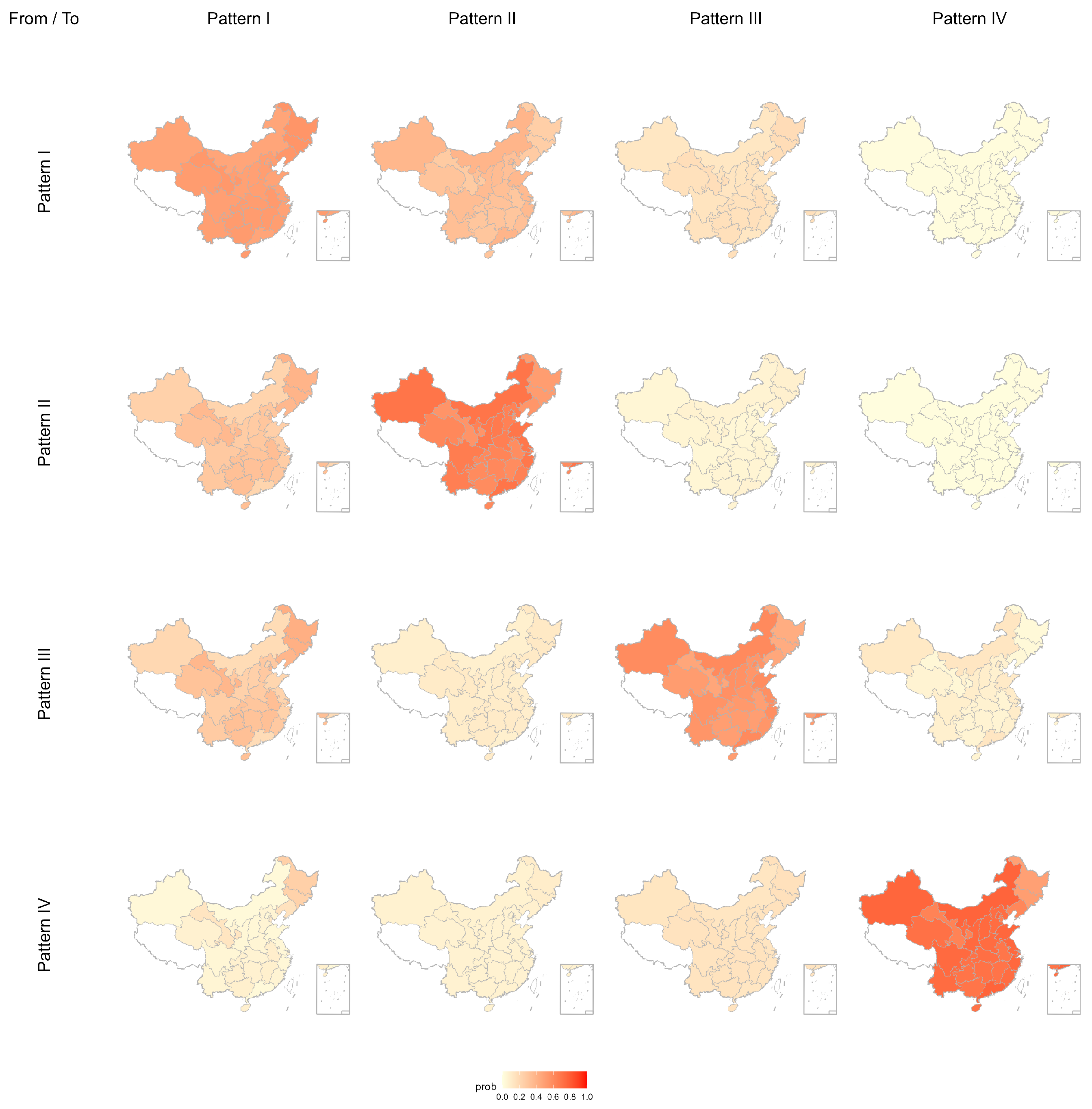
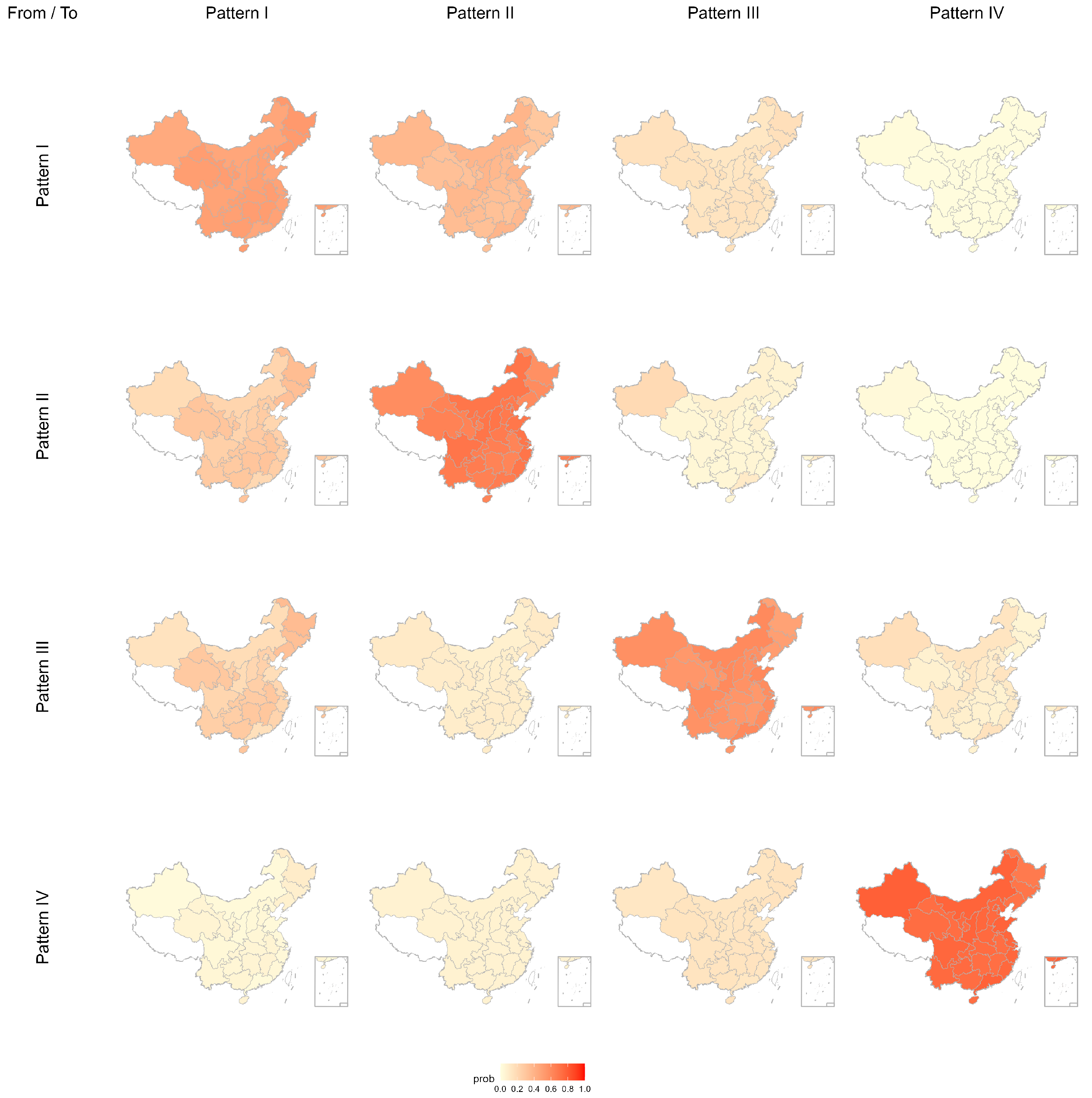
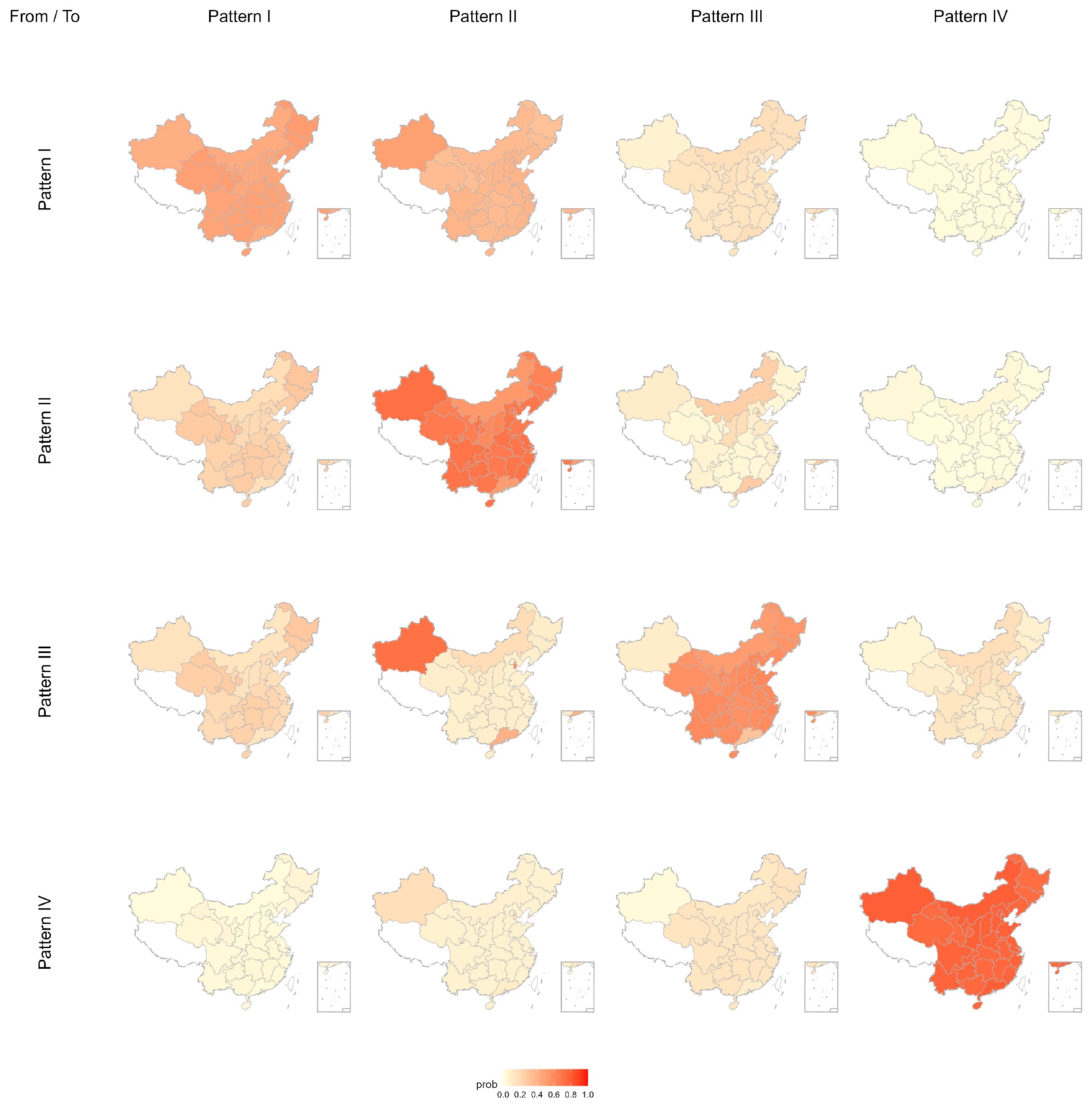
Moreover, to better illustrate the combined influence of GDP growth rate, population growth rate, and energy investment on carbon emission pattern transitions, we plotted spatial distribution maps of transition probabilities (Figure 4, Figure 5 and Figure 6), where darker shading indicates higher probabilities and lighter shading indicates lower probabilities.

Combining the self-transition probabilities reported in Table 13 with these maps at the 0.25, 0.50, and 0.75 quantile levels reveals a clear trend of increasing spatial stability for the medium and high emission patterns as the aggregated covariate index rises.

At the 0.25 quantile level (Figure 4), Pattern I and Pattern III exhibit self-transition probabilities of 0.515 and 0.518, respectively, corresponding to moderate shading; Pattern II rises to 0.612 with darker shading; and Pattern IV attains 0.715, showing the darkest shading and widest coverage, indicating relatively strong persistence under low covariate pressure. At the 0.50 quantile level (Figure 5), Pattern I declines to 0.490 with slightly lighter shading; Pattern II and Pattern III increase to 0.678 and 0.572 respectively, both showing marked deepening of shading; and Pattern IV reaches 0.749 with its darkest areas expanding substantially, reflecting enhanced spatial stability of the medium and high emission categories under moderate covariate pressure. At the 0.75 quantile level (Figure 6), Pattern I further decreases to 0.466, maintaining lighter shading; Pattern II and Pattern III rise to 0.696 and 0.602; and Pattern IV peaks at 0.769, all three exhibiting the darkest shading, with Pattern III and Pattern IV covering the largest area.

This pattern demonstrates that under high covariate pressure the medium and high emission categories retain their states more robustly than under lower pressures. Overall, the spatial patterns align closely with the numerical values, highlighting how covariate intensity shapes the persistence of emission patterns.

Table 14. Transition intensity matrix: aggregated covariate index.

0.25 Quantile Level
From/To	Pattern I	Pattern II	Pattern III	Pattern IV
Pattern I	−0.986	0.641	0.342	0.003
	(−0.986–−0.986)	(0.418–0.956)	(0.197–0.569)	(0.000–2463.532)
Pattern II	0.660	−0.675	0.001	0.014
	(0.473–0.942)	(−0.675–−0.675)	(0.000–0.496)	(0.002–0.126)
Pattern III	0.672	0.000	−0.779	0.106
	(0.368–1.227)	(0.000–0.325)	(−0.779–−0.779)	(0.023–0.483)
Pattern IV	0.019	0.087	0.241	−0.347
	(0.000–2674.964)	(0.008–0.934)	(0.076–0.742)	(−0.347–−0.347)
0.50 Quantile Level
From/To	Pattern I	Pattern II	Pattern III	Pattern IV
Pattern I	−0.978	0.698	0.279	0.001
	(−0.978–−0.978)	(0.510–0.960)	(0.176–0.449)	(0.000–3555.721)
Pattern II	0.524	−0.543	0.009	0.010
	(0.376–0.743)	(−0.543–−0.543)	(0.000–0.256)	(0.001–0.120)
Pattern III	0.491	0.000	−0.639	0.148
	(0.331–0.740)	(0.000–0.375)	(−0.639–−0.639)	(0.063–0.360)
Pattern IV	0.002	0.088	0.214	−0.304
	(0.000–8608.288)	(0.016–0.444)	(0.088–0.508)	(−0.304–−0.304)
0.75 Quantile Level
From/To	Pattern I	Pattern II	Pattern III	Pattern IV
Pattern I	−0.987	0.756	0.230	0.001
	(−0.987–−0.987)	(0.545–1.026)	(0.119–0.461)	(0.000–2161.343)
Pattern II	0.420	−0.497	0.070	0.007
	(0.275–0.657)	(−0.497–−0.497)	(0.014–0.330)	(0.000–0.221)
Pattern III	0.364	0.002	−0.568	0.203
	(0.196–0.646)	(0.000–0.713)	(−0.568–−0.568)	(0.110–0.413)
Pattern IV	0.000	0.089	0.192	0.000
	(0.000–11861.251)	(0.025–0.353)	(0.080–0.456)	(−0.281–−0.281)

Note: 95% confidence intervals are shown in parentheses; due to rounding, row sums may not equal exactly one.

presents the transition intensity matrix using ACI as the covariate, illustrating how instantaneous transition intensities among emission patterns vary across quantile levels. As the quantile level increases from the lower quartile to the median, the instantaneous transition rate from Pattern II to Pattern III exhibits a moderate upward trend; further ascent to the upper quartile induces a marked acceleration in this rate, signifying an enhanced propensity for provinces to migrate into higher-emission regimes under elevated ACI.

Collectively, these findings indicate that in contexts of vigorous economic expansion, demographic growth, and intensified energy investment, provincial emission trajectories predominantly shift toward higher emission categories before stabilizing at elevated levels. Furthermore, once high-emission states become established, they demonstrate substantial persistence and a low likelihood of downward migration, underscoring their intrinsic stability and resistance to reversal.

6. Concluding Remarks

This study applies k-means clustering to CO₂ emission data from 30 Chinese provinces between 2000 and 2021, identifying four representative emission patterns. A discrete endogenous Markov chain model is then employed to examine the dynamic evolution of these patterns and the factors influencing their transitions. The empirical results show that GDP growth substantially increases the probability of transitioning between emission states, thereby weakening the persistence of existing patterns. In contrast, population growth and energy investment tend to reinforce state stability. These findings highlight the differentiated impacts of socioeconomic variables on the evolution of emission trajectories.

The results offer valuable implications for emission mitigation policy. In contexts of rapid economic growth, fiscal incentives, technological upgrading, and infrastructure optimization may facilitate downward transitions to lower-emission regimes. In contrast, areas characterized by demographic inertia or investment rigidity may require long-term structural adjustments to enable sustained emission reduction. Moreover, the direction of energy investment plays a significant role in shaping transition dynamics. Policies should aim to redirect capital toward renewable energy and away from fossil intensive infrastructure to avoid carbon lock-in and enhance mitigation adaptability.

This study underscores the importance of integrating economic, demographic, and investment dimensions into carbon governance and advocates for a data driven, multifactor approach to understanding emission transitions.

Although this study offers a comprehensive analysis of emission patterns and their determinants, several limitations should be addressed in future work. First, the covariate set is relatively narrow; subsequent research should incorporate additional factors such as industrial structure and technological innovation and should combine the newly added variables with the original covariates in various configurations to conduct integrated analyses. Second, the application of spatial econometric techniques such as spatial autoregressive models or spatial error models could more accurately capture interprovincial spillovers and spatial dependence. In addition, identifying province-level heterogeneity in transition mechanisms represents a key direction for future research, which would enable the formulation of more precise and actionable subnational policy recommendations. Finally, extending the dataset to include the most recent observations and linking transition probabilities from higher to lower emission clusters under specified conditions to targeted policy interventions would enhance the timeliness of the results and improve the practical relevance of regional policy recommendations.

References

1. Li, Q. The view of technological innovation in coal industry under the vision of carbon neutralization. Int. J. Coal Sci. Technol. 2021, 8, 1197–1207. [Google Scholar] [CrossRef]
2. Kocak, E.; Alnour, M. The path to China’s zero-carbon target: Implications for the relationship between de-coal, economic output, and carbon dioxide emissions. Sustain. Dev. 2025, in press. [Google Scholar] [CrossRef]
3. Kao, X.; Liu, Y.; Wang, W.; Wen, Q.; Zhang, P. The pressure of coal consumption on China’s carbon dioxide emissions: A spatial and temporal perspective. Atmos. Pollut. Res. 2024, 15, 102188. [Google Scholar] [CrossRef]
4. International Energy Agency (IEA). CO2 Emissions in 2023; IEA: Paris, France, 2024; Licence: CC BY 4.0; Available online: https://www.iea.org/reports/co2-emissions-in-2023 (accessed on 1 March 2024).
5. Cai, X.; Xiang, H.; Zheng, H. Impact of energy consumption patterns on peak emissions in China’s carbon neutralisation process. Energy Strategy Rev. 2024, 55, 101501. [Google Scholar] [CrossRef]
6. Yang, Z.; Zhang, M.; Liu, L.; Zhou, D. Can renewable energy investment reduce carbon dioxide emissions? Evidence from scale and structure. Energy Econ. 2022, 112, 106181. [Google Scholar] [CrossRef]
7. Yuan, R.; Rodrigues, J.F.D.; Tukker, A.; Behrens, P. The statistical projection of global GHG emissions from a consumption perspective. Sustain. Prod. Consum. 2022, 34, 318–329. [Google Scholar] [CrossRef]
8. Gui, D.; He, H.; Liu, C.; Han, S. Spatio-temporal dynamic evolution of carbon emissions from land use change in Guangdong Province, China, 2000–2020. Ecol. Indic. 2023, 156, 111131. [Google Scholar] [CrossRef]
9. Wang, H.; Yu, X. Carbon dioxide emission typology and policy implications: Evidence from machine learning. China Econ. Rev. 2023, 78, 101941. [Google Scholar] [CrossRef]
10. Jiménez-Preciado, A.L.; Cruz-Aké, S.; Venegas-Martínez, F. Identification of Patterns in CO2 Emissions among 208 Countries: Clustering Combined with PCA and Non-Linear t-SNE Visualization. Mathematics 2024, 12, 2591. [Google Scholar] [CrossRef]
11. He, Y.; Xing, Y.; Zeng, X.; Ji, Y.; Hou, H.; Zhang, Y.; Zhu, Z. Factors influencing carbon emissions from China’s electricity sector: Analysis using the combination of LMDI and K-means clustering. Environ. Impact Assess. Rev. 2022, 93, 106724. [Google Scholar] [CrossRef]
12. Dong, F.; Wang, P.; Li, W. A study on the two-level allocation of carbon emission quotas in China at the provincial level. Environ. Sci. Pollut. Res. 2024, 31, 3669–3695. [Google Scholar] [CrossRef]
13. Liu, F.; Tang, L.; Liao, K.; Ruan, L.; Liu, P. Spatial distribution and regional difference of carbon emissions efficiency of industrial energy in China. Sci. Rep. 2021, 11, 19419. [Google Scholar] [CrossRef]
14. Wen, L.; Huang, L. Analysis of influencing factors of Chinese provincial carbon emissions based on projection pursuit model and Markov transfer matrix. Int. J. Climate Change Strateg. Manag. 2019, 11, 406–423. [Google Scholar] [CrossRef]
15. Wu, J.; Zhao, R.; Sun, J. State transition of carbon emission efficiency in China: Empirical analysis based on three-stage SBM and Markov chain models. Environ. Sci. Pollut. Res. 2023, 30, 117050–117060. [Google Scholar] [CrossRef]
16. Chen, J.C.; Wu, Y.J. Discrete-time Markov chain for prediction of air quality index. J. Ambient Intell. Hum. Comput. 2020, 11, 5033–5045. [Google Scholar] [CrossRef]
17. Huang, L.; Geng, X.; Liu, J. Study on the spatial differences, dynamic evolution and convergence of global carbon dioxide emissions. Sustainability 2023, 15, 5329. [Google Scholar] [CrossRef]
18. Putter, H.; Fiocco, M.; Geskus, R.B. Tutorial in biostatistics: Competing risks and multi-state models. Stat. Med. 2007, 26, 2389–2430. [Google Scholar] [CrossRef] [PubMed]
19. Yuan, M.; Xu, C.; Fang, Y. The transitions and predictors of cognitive frailty with multi-state Markov model: A cohort study. BMC Geriatr. 2022, 22, 550. [Google Scholar] [CrossRef]
20. Yu, S.; Wei, Y.-M.; Fan, J.; Zhang, X.; Wang, K. Exploring the regional characteristics of inter-provincial CO2 emissions in China: An improved fuzzy clustering analysis based on particle swarm optimization. Appl. Energy 2012, 92, 552–562. [Google Scholar] [CrossRef]
21. Inekwe, J.; Maharaj, E.A.; Bhattacharya, M. Drivers of carbon dioxide emissions: An empirical investigation using hierarchical and non-hierarchical clustering methods. Environ. Ecol. Stat. 2020, 27, 1–40. [Google Scholar] [CrossRef]
22. Hu, J.; Chen, J.; Zhu, P.; Hao, S.; Wang, M.; Li, H.; Liu, N. Difference and cluster analysis on the carbon dioxide emissions in China during COVID-19 lockdown via a complex network model. Front. Psychol. 2022, 12, 795142. [Google Scholar] [CrossRef]
23. Wang, W.; Tang, Q.; Gao, B. Exploration of CO2 emission reduction pathways: Identification of influencing factors of CO2 emission and CO2 emission reduction potential of power industry. Clean Technol. Environ. Policy 2023, 25, 1589–1603. [Google Scholar] [CrossRef]
24. MacQueen, J. Some methods for classification and analysis of multivariate observations. In Proceedings of the Fifth Berkeley Symposium on Mathematical Statistics and Probability; University of California Press: Berkeley, CA, USA, 1967; Volume 1: Statistics, pp. 281–298. [Google Scholar]
25. Kijewska, A.; Bluszcz, A. Research of varying levels of greenhouse gas emissions in European countries using the k-means method. Atmos. Pollut. Res. 2016, 7, 935–944. [Google Scholar] [CrossRef]
26. Kim, C.; Piger, J.; Startz, R. Estimation of Markov regime-switching regression models with endogenous switching. J. Econom. 2008, 143, 263–273. [Google Scholar] [CrossRef]
27. Hwu, S.-T.; Kim, C.-J.; Piger, J. An n-state endogenous markov-switching model with applications in macroeconomics and finance. Macroecon. Dyn. 2021, 25, 1937–1965. [Google Scholar] [CrossRef]
28. Peng, X.; Zhou, H.; Luo, L. Time-consistent investment strategy for a DC pension plan with hidden Markov regime switching. J. Comput. Appl. Math. 2023, 425, 115058. [Google Scholar] [CrossRef]
29. Azevedo, V.G.; Sartori, S.; Campos, L.M. CO2 emissions: A quantitative analysis among the BRICS nations. Renew. Sust. Energy Rev. 2018, 81, 107–115. [Google Scholar] [CrossRef]
30. Marjanović, V.; Milovančević, M.; Mladenović, I. Prediction of GDP growth rate based on carbon dioxide (CO2) emissions. J. CO2 Util. 2016, 16, 212–217. [Google Scholar] [CrossRef]
31. Wang, Y.; Kang, Y.; Wang, J.; Xu, L. Panel estimation for the impacts of population-related factors on CO2 emissions: A regional analysis in China. Ecol. Indic. 2017, 78, 322–330. [Google Scholar] [CrossRef]
32. Shaari, M.S.; Abidin, N.Z.; Ridzuan, A.R. The impacts of rural population growth, energy use and economic growth on CO2 emissions. Int. J. Energy Econ. Policy 2021, 11, 553–561. [Google Scholar] [CrossRef]
33. Yu, Y.; Deng, Y.; Chen, F. Impact of population aging and industrial structure on CO2 emissions and emissions trend prediction in China. Atmos. Pollut. Res. 2018, 9, 446–454. [Google Scholar] [CrossRef]
34. Li, J.; Li, S. Energy investment, economic growth and carbon emissions in China—empirical analysis based on spatial Durbin model. Energy Policy 2020, 140, 111425. [Google Scholar] [CrossRef]
35. Kuang, H.; Akmal, Z.; Li, F. Measuring the effects of green technology innovations and renewable energy investment for reducing carbon emissions in China. Renew. Energy 2022, 197, 1–10. [Google Scholar] [CrossRef]
36. Syakur, M.A.; Khotimah, B.K.; Rochman, E.M.; Satoto, B.D. Integration k-means clustering method and elbow method for identification of the best customer profile cluster. IOP Conf. Ser. Mater. Sci. Eng. 2018, 336, 012017. [Google Scholar] [CrossRef]
Figure 1. D-index variation across different numbers of clusters.
Climate 13 00165 g001
Figure 2. Second difference of D-index values.
Climate 13 00165 g002
Figure 3. Carbon emission clustering patterns in Chinese provinces (2021).
Climate 13 00165 g003
Figure 4. Spatial distribution of transition probabilities: aggregated covariate index (0.25 quantile level).
Climate 13 00165 g004
Figure 5. Spatial distribution of transition probabilities: aggregated covariate index (0.5 quantile level).
Climate 13 00165 g005
Figure 6. Spatial distribution of transition probabilities: aggregated covariate index (0.75 quantile level).
Climate 13 00165 g006