Should We Use Quantile-Mapping-Based Methods in a Climate Change Context? A “Perfect Model” Experiment

Abstract

This study assesses the use of Quantile-Mapping methods for bias correction and downscaling in climate change studies. A “Perfect Model Experiment” is conducted using high-resolution climate simulations as pseudo-references and coarser versions as biased data. The focus is on European daily temperature and precipitation under the RCP 8.5 scenario. Six methods are tested: an empirical Quantile-Mapping approach, the “Cumulative Distribution Function—transform” (CDF-t) method, and four CDF-t variants with different parameters. Their performance is evaluated based on univariate and multivariate properties over the calibration period (1981–2010) and a future period (2071–2100). The results show that while Quantile Mapping and CDF-t perform similarly during calibration, significant differences arise in future projections. Quantile Mapping exhibits biases in the means, standard deviations, and extremes, failing to capture the climate change signal. CDF-t and its variants show smaller biases, with one variant proving particularly robust. The choice of discretization parameter in CDF-t is crucial, as the low number of bins increases the biases. This study concludes that Quantile Mapping is not appropriate for adjustments in a climate change context, whereas CDF-t, especially a variant that stabilizes extremes, offers a more reliable alternative.

1. Introduction

Over the last few decades, scientists have attempted to model, quantify, and understand the potential impacts of climate change. To investigate these impacts, various hydrological, agricultural, and, more generally, environmental “impact models” have been developed (e.g., [1,2]). Although such models can be different regarding their goals, underlying assumptions, and functioning, they all rely on the use of climate simulations of climate variables, such as temperature and precipitation, as inputs to simulate impacts (e.g., in terms of river flows, crop yields, etc.). Therefore, the realism and robustness of climate simulations are essential, both over historical and future periods and scenarios of interest, to obtain confidence in the modeled impacts (e.g., [3]).

However, because global climate simulations usually have a relatively low spatial resolution, a major drawback is that they are not designed to provide local information. Indeed, Global Climate Models (GCMs) have a mean resolution of approximately 150 × 150 km, whereas most impact models operate at a much more local scale, from a watershed or crop region to a specific location represented by a weather station. Thus, the spatial resolution of GCM simulations is not adapted to the input resolution required by impact models (e.g., [1,4,5]). Regional Climate Models (RCMs) have been developed to simulate climate variables at a higher spatial resolution over a large domain. RCMs are forced by GCM simulations and downscale them physically based on regional-scale atmospheric dynamics equations [6]. They can now reach resolutions of up to the kilometer scale. However, this RCM-based downscaling approach has several disadvantages. First, RCMs require intensive computing resources; thus, they are generally applied only to a subset of available GCM simulations over some regions and are not run by impact modelers themselves. Indeed, beyond the necessary computing resources—which are increasingly accessible—RCM codes are not always open source (as climate modeling centers do not necessarily make them publicly available); they require a high level of expertise in climate physics and involve handling large volumes of input and output data. Moreover, RCM simulations are not necessarily available at the spatial resolution required by impact models. In addition, even at an appropriate spatial resolution, RCM simulations often have statistical biases with respect to reference data (e.g., from reanalyses or weather stations), and these biases must be removed before use in impact studies. The last two points (i.e., unadapted resolution and/or biases) motivated the development of statistical downscaling (SD) and bias correction (BC) methods. Despite their conceptual proximity, it is essential to distinguish between them.

Theoretically, the SD and BC methods have two distinct objectives: SD focuses on changes in resolution, whereas BC removes biases, without necessarily modifying the resolution. In practice, BC methods can be applied to perform downscaling, considering the disagreement between large-scale simulations and local-scale references as a bias to be corrected. Indeed, when applying a bias correction technique—such as a Quantile-Mapping-based method—to low-resolution GCM simulations at a given grid cell with respect to a reference local-scale time series (e.g., from a high-resolution reanalysis or a weather station), bias-corrected station-scale projections are provided. Hence, even though there is no explicit statistical downscaling model linking the predictors (i.e., low-resolution variables) to the predictands (i.e., local variables), the bias correction procedure effectively downscales the coarse-resolution data using the reference local distribution. However, BC methods applied for downscaling purposes can suffer from various drawbacks [7], such as overly uniform temporal properties across space or unrealistic spatial dependencies at local and regional scales. Another difference between SD and BC is methodological. Most SD methods (i.e., focusing on changes in resolution) are calibrated using reanalyses for large-scale data to be downscaled. They then assume that climate simulations have statistical properties similar to those from reanalyses and can thus be used as predictors in the SD model. Such an approach is called “Perfect-Prognosis” (PP) (e.g., [8,9]). Many PP approaches exist, ranging from linear or non-linear regressions (e.g., [10]), including neural network methods (e.g., [11]), to stochastic downscaling methods that specifically model the variability/uncertainty of local-scale data (e.g., [12,13,14]), using weather-typing SD methods relying on large-scale circulation regimes (e.g., [15]). In contrast, BC methods do not assume that climate simulations have statistical properties similar to those from reanalyses and therefore do not use reanalyses for calibration. These methods directly relate the statistical properties (or distributions) from the climate simulations to those from the reference data in order to transform (i.e., correct or adjust) the simulations in such a way that their properties are similar to those of the reference. Such an approach is referred to as “Model Output Statistics” (MOS, e.g., [8,16]). In practice, MOS approaches are used regularly for downscaling. The most employed MOS method in this context is certainly the “quantile-mapping” method (e.g., [17,18,19])—hereafter referred to as QM—whose target is to adjust the whole univariate distribution (i.e., not only the mean and variance but also all moments of higher order, as well as any percentile) of a given climate variable. For a variable X (e.g., temperature) from model G ($X_G$) or from the reference dataset ($X_{\mathrm{ref}}$) with cumulative distribution functions (CDFs) $F_{\mathrm{ref}}$ and $F_G$, the QM method corrects/downscales the simulation value $x_G$ (i.e., provides a value $x_{ref}$) based on the following formulation:

$$x_{\mathrm{ref}}=F_{\mathrm{ref}}^{-1}\left(F_G\left(x_G\right)\right),$$

(1)

where $F^{-1}$ is the inverse CDF of F. As this method is simple, easy to implement, fast to run, and provides relatively robust corrections, it has received considerable interest and has been applied to downscale climate simulations to provide input to many impact models (e.g., [3,20,21]). However, QM has one major limitation when the corrected simulations exhibit a strong change with respect to the calibration period. Indeed, to correct or downscale the model simulations from the projection period ($X_{G,\mathrm{proj}}$), QM computes the value of the calibration CDF applied to these simulations ($F_{G,\mathrm{cal}}\left(X_{G,\mathrm{proj}}\right)$) before applying the reference inverse CDF $F_{\mathrm{ref},\mathrm{cal}}^{-1}$ to obtain the corrected/downscaled value. However, in the context of climate change, it is expected that the CDFs from the calibration and projection periods will differ. Hence, the computation of $F_{G,\mathrm{cal}}\left(X_{\mathrm{proj}}\right)$ is not necessarily appropriate because the variable $X_{proj}$ is not projected onto the appropriate CDF over the correct period [22,23]. A potential consequence in the context of climate change is that QM can project inappropriate corrections, inconsistent with the climate change signal given by the climate model to be downscaled.

Hence, Michelangeli et al. [22] developed a variant called the “Cumulative Distribution Function transform” (CDF-t) based on an estimation of the local-scale future distribution over the target projection period. This estimation is performed before QM is applied over the target period itself [23]. Over the last decade, several variants of CDF-t have been proposed, such as those focusing on extremes [24] or designed for precipitation [25], and have been applied in various studies (e.g., [26,27,28,29,30,31,32,33,34], among others).

Recently, Lanzante et al. [35] proposed an extension of the CDF-t method to improve the correction of simulations in the tail of the distribution (i.e., extremes). This updated version of CDF-t was applied by Noël et al. [34] to five daily climate variables (mean, maximum and minimum air temperatures, precipitation, and mean near-surface wind speed) from 21 CMIP5 GCMs from 1950 to 2100 under two future greenhouse gas emission scenarios (RCP 4.5 and RCP 8.5) and recently to surface temperature and precipitation from 5 CMIP6 GCMs for two emission scenarios [36]. Corrections were made with respect to ERA5 [37] and ERA5-Land [38] reanalyses at 0.25° × 0.25° and 0.10° × 0.10° spatial resolutions, respectively. Although the generated corrections were quality-checked with respect to reanalyses over the historical period, it is important to understand how this updated CDF-t method behaves in a climate change context and how it compares with respect to a more traditional QM method and the native CDF-t method (i.e., without the extension accounting for the extremes). Moreover, both the native CDF-t method and its recent extension have various parameters that must be set by users. Investigating the influence of these parameters in the context of climate change is of great interest for practical downscaling applications of future climate projections to guide the selection of the best set of parameters.

Despite recent improvements and extensions of the Quantile-Mapping method, the basic QM approach is still largely applied in the context of climate change, including the investigation of changes in high quantiles (e.g., [39]). Hence, the goals of this study are (i) to evaluate whether the QM method is appropriate within a climate change context, compared to its CDF-t extensions, and (ii) to assess the recent variants of CDF-t, together with the influences of its parameters. To perform these evaluations, we adopt a “Perfect Model Experiment” (PME) setting, which relies on high-resolution simulations used as reference or pseudo-observations (e.g., [35,40,41]), thus making them available over future periods, for example, up to the end of the 21st century. In this setting, the “references” are simply the original data of the high-resolution simulation, whereas the “model simulation” is a coarser version of the same data obtained through upscaling on a coarser grid. This produces a mismatch in the spatial resolution representative of the downscaling that must be applied, thus providing data for the historical (i.e., calibration) period, as well as for the future (i.e., projection) state. As such, the more distant the future period, the more affected it is by climate change, and the better the evaluation of methodological errors implicit in SD methods in a non-stationarity context [42,43].

The remainder of this article is organized as follows: Section 2 describes the data and downscaling procedure; Section 3 details the experimental design of the tested BC methods, as well as the metrics used for the evaluations; Section 4 presents the results in terms of metrics categorized into marginal, extreme, temporal, and multivariate criteria; and finally, conclusions and discussions are provided in Section 5.

2. Data and Methods

2.1. Data

To set up our Perfect Model Experiment (PME), high-resolution climate simulations were first selected to serve as pseudo-references for present and future climates. Next, we use daily simulations from the EURO-CORDEX experiments [44], which have a 0.11° × 0.11° spatial resolution and are available up to the end of the 21st century, over a European domain defined as approximately [20° E, 50° W] × [30° N, 70° N]. Hence, these CORDEX pseudo-references allow us to test the ability of the bias correction to be performed in a climate change context and analyze its capability to account for model changes from the early to the late century.

In this work, we chose to focus on the European daily surface temperature and precipitation under the RCP 8.5 scenario [45]. Indeed, these two variables are central to many impact studies, and RCP8.5 is the highest CO₂ emission scenario, producing the largest changes by the end of the 21st century. From the Euro-CORDEX archive, we arbitrarily selected simulations corresponding to the “Weather Research and Forecasting” RCM (WRF, [46]) forced by the IPSL GCM [47]. The historical run covers the 1951–2005 period, while the projections cover the 2006–2100 time period under the RCP8.5 scenario. Hereafter, this high-resolution dataset is referred to as the “reference”.

Then, the large-scale simulations to be downscaled/bias-corrected, that is, serving as a proxy for a GCM simulation, were obtained by upscaling the above-defined reference simulations to a coarse GCM spatial resolution of 2° × 2°. This was performed with a conservative scheme using the Climate Data Operators software package [48]. The spatial resolution change ratio was purposely high (2° compared to 0.11°, which is equivalent to about 1/330 of the surface ratio) to allow for the testing of the method in the context of high-resolution references for model downscaling, such as the recent ERA5-Land reanalysis dataset (0.1°), which is often used as a reference for downscaling (e.g., [36]). In the following section, because this larger-scale dataset is used as a proxy of the model data to be downscaled, it is referred to as “model data”.

2.2. Downscaling Methodologies

Two primary methods are tested in this study. The first is the Quantile Mapping (QM) method (e.g., [17,18,19]), which is detailed in Section 1 and based on Equation (1). This method is widely used in the climate literature to downscale or adjust climate simulations; it serves as a benchmark. The second method is the Cumulative Distribution Function transform (CDF-t) method, from which several variants are tested (see the next section). If X denotes the random variable representing the modeled variable to be corrected and Y is the random variable representing the reference variable, the cumulative distributions $F_{Yp}$ and $F_{Xp}$ are estimated by CDF-t from the random variables $Y_p$ and $X_p$ over the projection (future) time period before applying a distribution-derived quantile map:

$$F_{Yp}\left(y_p\right)=F_{Xp}\left(x_p\right)\iff y_p=F_{Yp}^{-1}\left(F_{Xp}\left(x_p\right)\right).$$

(2)

If $F_{Xp}$ can be directly modeled (either parametrically or not) from the model data to be corrected in the projection period, the modeling of $F_{Yp}$ is based on the assumption that a mathematical transformation T allows us to go from $F_{Xc}$ to $F_{Yc}$, the distributions of the random variables $Y_c$ and $X_c$ in the calibration period:

$$T\left[F_{Xc}\left(z\right)\right]=F_{Yc}\left(z\right)$$

(3)

for any z, and T is still valid in the projection period, that is,

$$T\left[F_{Xp}\left(z\right)\right]=F_{Yp}\left(z\right).$$

(4)

By replacing z with $F_{Xc}^{-1}\left(u\right)$, where u is any probability in $[0,1]$, we obtain

$$T\left(u\right)=F_{Yc}\left[F_{Xc}^{-1}\left(u\right)\right],$$

(5)

corresponding to a simple definition of T. Inserting this definition (Equation (5)) into Equation (4) leads to the modeling of $F_{Yp}$ as

$$F_{Yp}\left(z\right)=F_{Yc}\left[F_{Xc}^{-1}\left[F_{Xp}\left(z\right)\right]\right].$$

(6)

By accounting both for the bias correction of the model distribution with respect to the reference one (via $F_{Yc}\circ F_{Xc}^{-1}$) and for the link between the historical and future model distributions (via $F_{Xc}^{-1}\circ F_{Xp}\left(z\right)$), Equation (6), at the heart of CDF-t, reflects the fact that this BC method accounts for the non-stationarity of the distributions under climate change. Once $F_{Xp}$ and $F_{Yp}$ are modeled, distribution-based Quantile Mapping is applied as in Equation (2). Hence, the CDF-t approach includes information regarding the distributions over the projection period by using the Quantile Mapping technique.

The bias correction method can significantly modify the occurrence and intensity of precipitation. Therefore, a specific treatment is applied for the correction of precipitation. The first filter is the management of occurrences by modifying the 0 values in the observed and modeled time series by very low values (Singularity Stochastic Removal approach; for more details, see [25]). The second filter considers the strong differences between the CDFs of the observations and the CDFs from the models. To improve the concordance of the CDFs, the modeled precipitation values are normalized using the maximum values of the observations time series ($M_{\mathrm{ref}}$) and the maximum values from the model data ($M_{\mathrm{Cmod}}$) for the calibration period (Equation (7)) and the projection period (Equation (8)) as follows:

$${\tilde{X}}_c=X_c·{\displaystyle \frac{M_{\mathrm{ref}}}{M_{\mathrm{Cmod}}}};$$

(7)

$${\tilde{X}}_p=X_p·{\displaystyle \frac{M_{\mathrm{ref}}}{M_{\mathrm{Cmod}}}}.$$

(8)

This normalization step aims to maximize the overlap between $F_{Xc}$—the distribution of the model simulation during the calibration period—and $F_{Yc}$—the distribution of the reference data over the same period. Indeed, Equation (6) involves computing $F_{Yc}\left(F_{Xc}^{-1}\left(v\right)\right)$, where v is the probability $F_{Xp}\left(z\right)$. If the domain of $F_{Xc}$ differs significantly from that of $F_{Yc}$, the CDF-t method becomes ineffective, as $F_{Yc}$ would then mostly return values equal to 0 (if it lies to the right of $F_{Xc}$) or 1 (if it lies to the left) [23,25]. This normalization can thus be interpreted as a pre-correction step before applying CDF-t. In the remainder of this study, the original CDF-t version of Michelangeli et al. [22] is used for both temperature and precipitation, with particular pre- and post-processing for precipitation to account for occurrence and intensity, as presented by Vrac et al. [25]. It is worth noting that CDF-t has only one fundamental parameter, which is the number of “cuts” for which quantiles are empirically estimated. This parameter is called NPAS in the code available online accessed on 2 July 2023, (https://cran.r-project.org/package=CDFt) and corresponds to the number of cuts of the quantiles. Although the value must be adjusted for each application depending on the region and variable, many users maintain a default value of 100. This default value can produce satisfactory results while maintaining a low computational time (the higher the NPAS, the higher the CPU time). However, in several cases, particularly for precipitation, a significantly higher value is required to achieve satisfactory results. Indeed, using a low NPAS value can lead to poor BC results and a poor performance [35]. For example, for a precipitation time series of approximately 1200 time steps, NPAS = 1000 is recommended as the minimum value and even higher for regions with a relatively dry climate. For this reason, the default value is set to 1000; however, as a rule of thumb, it is recommended that the NPAS parameter should be at least 3/4 of the length of the reference time series.

Remapping is a mandatory preliminary task required in downscaling methodologies based on Quantile Mapping approaches (such as QM and CDF-t). It consists of spatially associating or interpolating coarse model data into a finer reference grid. We used Climate Data Operators (CDOs, [48]) to remap daily coarse model data from 2° to 0.11° on the reference grid. The daily mean temperature was interpolated directly using a bi-linear method, while daily precipitation was interpolated sequentially (with intermediate resolutions of 1.5° and 0.75°), as in Noël et al. [34], on the reference grid with a conservative method.

3. Experimental Design

The core principle of the proposed Perfect Model Experiment is to use (1) high-resolution climate simulations as the reference and (2) degraded (i.e., lower-resolution) simulations as the biased data requiring correction. This setup enables the evaluation of bias correction methods in a context of pronounced climate change—a context that cannot be adequately reproduced using reanalyses or even historical simulation or reanalysis data alone due to the relatively short time span and weaker climate signals.

Two points should be considered when adopting this PM experiment: First, by construction, the biases in the model data with respect to the references are only due to spatial smoothing because both datasets are the same but at different spatial resolutions. However, in practical downscaling with GCM simulations, additional biases, even at the synoptic scale, can be relatively large (e.g., [49]). Second, by construction, the model and reference proxies have the same temporality; that is, they are temporally matched. This allows for the use of classical time-series statistics (such as correlation) as evaluation metrics.

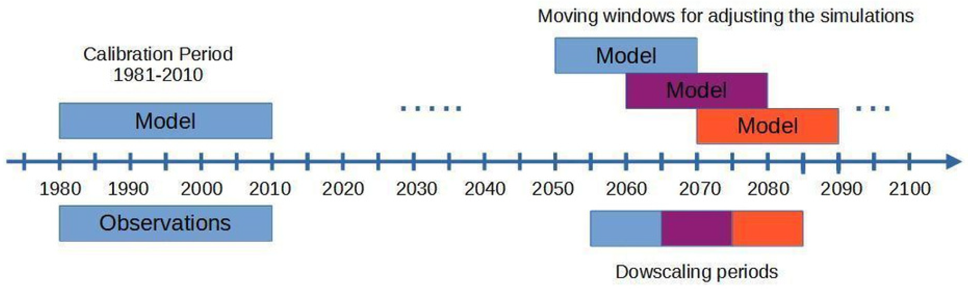
3.1. Calibration and Validation Setup

In the remainder of this study, the calibration period is taken as 1981–2010, while the projection period (i.e., the period for which we want to downscale the large-scale simulations) is 2011–2100. In such applications, the way downscaling is applied to multidecadal time series is important. Typically, statistical techniques use a calibration period of 20 or 30 years and are applied to future periods of similar lengths. Climate simulations extend to longer periods, and downscaled periods can reach 100 years or more. Thus, it is necessary to process series that are longer than the calibration period. One way to do so is to divide the 100-year projection period into sub-periods with a length equivalent to the calibration period and to apply the downscaling to each sub-period. However, this approach can generate discontinuities at the sub-period junctions. Here, we apply the QM and CDF-t methods with a double-moving-window approach (illustrated in Figure 1) to avoid—or at least reduce—such discontinuities between periods. This approach uses a first (external) window of 20 years to fit the distributions required to apply CDF-t but then downscales the simulations only within a 10-year (internal) window at the center of the time window (except for the first and last periods, which also include the corresponding five years at the beginning and end). The window is then moved 10 years forward (i.e., the size of the internal window) to downscale the following decade. Here, a 20–10 window is used because future time series have a strong temperature trend; however, other choices are possible. The next section explores the influence of these choices.

3.2. Experiments

Based on this framework, we conduct several experiments in which the future values of the coarse data are downscaled at the reference data grid using historical reference and coarse data for calibration. Hence, the downscaled data can be evaluated against the reference data over the future period. The calibration period is 1981–2010, and a double moving window of 20–10 is applied to downscale the 2006–2100 time series of the coarse data (as in [34,36]). Six downscaling methods based on Quantile Mapping are tested. The first experiment corresponds to a simple QM method [18]. The second method is the original CDF-t method [25], whereas the other four methods correspond to recent variants of CDF-t [35]. As a reminder, based on the PM Experiment, one main goal is to evaluate the capability of these methods to perform adequately in the context of climate change. All six experiments are described below and are conducted using the same procedure and parameters unless specified otherwise.

The first experiment, called QM, is conducted using the simple Quantile Mapping method [19], as detailed in Section 1 and Equation (1).

The second experiment uses the CDF-t method (see Section 2.2), as described by Michelangeli et al. [22] for temperature and Vrac et al. [25] for precipitation, with the NPAS parameter set to 1000 for temperature and 5000 for precipitation.

The subsequent experiments are recent variants of the CDF-t method:

• The third experiment, called LAN, is the CDF-t method with a modification of the treatment of the extreme quantiles, as described by Lanzante et al. [35]. This modification involves two parameters, aiming at correcting the tail of the distribution:

  –

  TLN (meaning “Tail length”), defined as the “number of tail points to be adjusted”;

  –

  NPT (meaning “lastN-points”), defined as “the number of ‘good points’ (i.e., those adjacent to the portion of a tail to be adjusted) averaged to determine the tail adjustment factor”.

  Here, in order to avoid potential instabilities in the tails of the corrected distribution (i.e., in the few smallest or highest downscaled values), the lowest and the highest TLN = 10 values of the data are all adjusted by the value $\Delta$, corresponding to the mean correction of the NPT = 10 values preceding the highest TLN values or following the lowest TLN values. In a more mathematical formulation, if $X_p^r$ is the model data to be downscaled ranked in increasing order and if $X_p^r\left(i\right)$ is the $i\mathrm{th}$ value of $X_p^r$ (i.e., the $i\mathrm{th}$ lowest value of $X_p$) and $Y_p^r\left(i\right)$ is the downscaled value obtained within the projection period (p), then for the adjustment of the lowest (i.e., left) tail of the distribution,

  $$\Delta ={\displaystyle \frac{1}{NPT}}\sum _{i=\mathrm{TLN}+1}^{i=\mathrm{TLN}+\mathrm{NPT}}[Y_p^r\left(i\right)-X_p^r\left(i\right)];$$

  (9a)

  while for the highest (i.e., right) tail of the distribution,

  $$\Delta ={\displaystyle \frac{1}{NPT}}\sum _{i=N-\mathrm{TLN}-\mathrm{NPT}+1}^{i=N-\mathrm{TLN}}[Y_p^r\left(i\right)-X_p^r\left(i\right)].$$

  (9b)
  The downscaled values for the first TLN points ($i=1,\dots ,\mathrm{TLN}$) and the last TLN points ($i=N-\mathrm{TLN}+1,\dots ,N$, where N is the total number of data points) are then obtained as

  $$Y_p^r\left(i\right)=X_p^r\left(i\right)+\Delta$$

  (10)

  based on the appropriate $\Delta$ value. This corresponds to a safeguard to prevent the most extreme points of the distribution from becoming numerical outliers. Figure 2 illustrates the procedure used in the LAN experiment for the upper tail of temperature in October and for the grid cell containing the city of Paris, with TLN = 5 data points and NPT = 10 data points for computing $\Delta$.
• The fourth experiment, called NPAS, is based on the LAN experiment by changing only the number of cuts of the quantiles and setting the variable $NPAS$ to 100 (i.e., instead of 1000 for temperature and 5000 for precipitation for the CDF-t and LAN experiments). This experiment is conducted to explore the sensitivity of the results to low $NPAS$ values.
• The fifth experiment, called MW, is also based on the LAN experiment but changes only the parameters of the moving window to 30–10 (instead of 20–10). This is done to test the effect of a longer (external) window period.
• Finally, the sixth and last experiment, called TLN, is also based on the LAN experiment, but the parameter TLN is set to 5. This is to test a smaller number of tail points to limit the change to 1% of the available data (900 data points; thus, five points for each tail) at the tails of the distribution.

Table 1. List of experiments and their characteristics according to the values used for the “Double-Moving-Window” approach, the NPAS parameter (number of cuts) of the CDF-t method, and the parameters TLN and NPT for smoothing the tails of the CDFs (see text for details).

Experiment	Double-Moving-Window (Ext.-Int. in Years)	NPAS (Temp–Prec)	TLN/NPT
QM	20–10	1000–5000	–/–
CDF-t	20–10	1000–5000	–/–
LAN	20–10	1000–5000	10/10
NPAS	20–10	100–100	10/10
MW	30–10	1000–5000	10/10
TLN	20–10	1000–5000	5/10

summarizes the experiments and their characteristics.

3.3. Metrics

The validation of downscaling methods is a multifaceted problem involving different aspects such as the representation of extremes or temporal and spatial structures. The VALUE project [50] developed a comprehensive list of indices and measures that allow for the proper evaluation of most of these aspects. In the present study, we consider a subset of the VALUE metrics shown in

Table 2. List of metrics and their definitions. T: temperature, P: precipitation, MD: marginal distribution, Ext: extremes, TP: temporal property, Sp: spatial, and InterVar: inter-variable. $(i,j)$ are grid-point coordinates.

Metric	Unit	Variable	Type	Calculation	Definition
Bias in the Mean	[°C, mm]	T&P	MD	$m_{X_{i,j}}-m_{Re{f}_{i,j}}$; m is the mean over 30 years; For precipitation, dry days < 1 mm/d are excluded.	Difference in mean value over a 30-year period per grid cell, ref. the minus experiment. For P, dry days are excluded.
Bias in the Std. Dev.	[°C, mm]	T&P	MD	${\mathrm{Std}}_{X_{i,j}}-{\mathrm{Std}}_{Re{f}_{i,j}}$; dry days < 1 mm/d excluded.	Difference in standard deviation over a 30-year period per grid cell. Dry days excluded for P.
Bias in Rainy Days	[days]	P	MD	$D_{X_{i,j}}-D_{Re{f}_{i,j}}$; D is the # of days with Pr > 1 mm.	Difference in the # of rainy days over a 30-year period per grid cell.
Root Mean Squared Error	[°C, mm]	T&P	MD	$\sqrt{\sum {(X_{i,j}-X_{Re{f}_{i,j}})}^2/n}$	Root Mean Squared Error on daily values over a 30-year period.
Bias in Q98	[°C, mm]	T&P	Ext	$Q{98}_{X_{i,j}}-Q{98}_{Re{f}_{i,j}}$; for P, dry days excluded.	Difference in the 98th percentile per grid cell. Dry days excluded for precipitation.
Bias in Q02	[°C, mm]	T&P	Ext	$Q{02}_{X_{i,j}}-Q{02}_{Re{f}_{i,j}}$; dry days excluded.	Difference in the 2nd percentile per grid cell. Dry days excluded for P.
Bias in Warm Days	[days]	T	Ext	$D_{X_{i,j}}-D_{Re{f}_{i,j}}$ where D is the # of days with T > 20 °C (spring/fall), 25 °C (summer), and 15 °C (winter).	Difference in the # of warm days per 30-year period.
Bias in Heavy Precip. Days	[days]	P	Ext	$D_{X_{i,j}}-D_{Re{f}_{i,j}}$ where D is the # of days with Pr > 20 mm.	Difference in the # of very heavy precipitation days over 30 years.
Pearson Corr.	[−]	T&P	TP	$\rho (X_{i,j},X_{Re{f}_{i,j}})$	Pearson correlation per grid cell over 30 years between the model and reference.
Bias in Lag-1 Autocorrelation	[−]	T	TP	${\rho }_1\left(X_{i,j}\right)-{\rho }_1(X_{Re{f}_{i,j}})$; with ${\rho }_1$ as the 1 day-lag autocorrelation.	Difference in 1-day lag autocorrelation per grid cell.
Bias in Persistence	[days]	P	TP	$S_{X_{i,j}}-S_{Re{f}_{i,j}}$; S = the mean wet spell duration.	Difference in mean wet spell duration over a 30-year period.
Bias in T-P Corr.	[−]	T&P	InterVar	${\rho }_{T,P}^X-{\rho }_{T,P}^{Ref}$ per grid cell.	Difference in Pearson correlation between T and P over 30 years.
Explained Variance	[%]	T&P	Sp	PCA on experiment results and PCA on references.	Comparison of explained variance from PCA.

(as in [11]) that cover the mean bias, some extreme quantiles, and temporal characteristics. A few other criteria are added to address the spatial and inter-variable characteristics to assess the performance of the downscaling method in reproducing the reference data at each point of the domain using the 30-year period over a historical period (1981–2010) and over the end of the century (2071–2100).

The first set of metrics addresses the characteristics of the marginal distribution. This comprises the bias of the mean and standard deviation for both variables. For precipitation, the number of rainy days is added as this is a fundamental climatological characteristic. Dry days are excluded from the calculation of precipitation of the first metric set. The mean bias over the future period allows us to evaluate the behavior of each experiment in a non-stationary context.

The second set addresses the ability to reproduce extreme values. It comprises both relative and absolute extremes. For both variables, the upper extremes are expressed as the 98% quantiles (Q98) and the lower extremes as the 2% quantiles (Q02). Note that, for precipitation, dry days are excluded from quantile computations. Consequently, the number of dry days is added as a metric. Upper absolute thresholds are also investigated for both variables as the number of days exceeding a given threshold (20 °C for spring and fall, 15 °C for winter, and 25 °C for summer) for temperature and 20 mm/day for precipitation (regardless of the season).

The third set of criteria evaluates temporal properties. The Pearson’s correlation coefficient and order-1 autocorrelation are used for both variables. We remind the reader that it makes sense to compute the correlations here because the time series of the downscaled and reference data are synchronous owing to the PME context. Usually, the seasonal cycle is removed in this type of approach to avoid a positive bias in performance and to focus on anomalies only. Here, we perform the analysis every month (see the next section); therefore, removing the seasonal cycle is not necessary. Regarding the computation of the first-order autocorrelation, the aim is to assess whether the correction methods alter this autocorrelation compared to the raw simulations (i.e., with no correction) and to determine if one bias correction method has a more significant impact than the others. For precipitation, instead of the order-1 autocorrelation, which is not easily interpretable due to the many dry days, we evaluate the mean length of the wet spells (i.e., persistence). These metrics—autocorrelation and persistence—are particularly relevant in impact studies across fields such as hydrology, health, and agriculture, where the timing and duration of events (e.g., heatwaves or dry spells) are often as critical as their intensity. They provide simple yet insightful summaries of event sequencing and temporal structures.

Finally, two additional metrics are considered: one to evaluate the spatial structure of each climate variable individually and another to assess the relationships between variables. To evaluate spatial structures, principal component analysis (PCA)—also known as Empirical Orthogonal Function (EOF) analysis—is applied separately to each variable. PCA is a statistical method used to identify dominant spatial patterns in the data and their associated temporal variations. In this study, it is used to extract the leading modes of variability from the bias-corrected datasets and compare them with those derived from the reference datasets. This comparison provides insights into how well the spatial structure of climate variability is preserved or modified after bias correction by decomposing the data into orthogonal functions that explain the maximum variance. Regarding the inter-variable assessment, Pearson correlation coefficients between temperature and precipitation are computed at each grid cell. Capturing realistic correlations between these variables is crucial, as many impacts across various sectors—such as agriculture, hydrology, and health—depend on their combined behaviors. For instance, hot and dry conditions can severely affect crop yields and water resources, whereas processes such as snowmelt and runoff are driven by both temperature and precipitation. Failing to account for their co-variability can result in inaccurate impact assessments. All criteria are defined in Table 2.

4. Results

The results of the six experiments—including the raw climate simulations, hereafter referred to as the “RAW” experiment—are shown over the calibration period (1981–2010) and over a validation period of similar length by the end of the century (2071–2100). For the sake of space, the results are provided and analyzed for October only (representative of the autumn season). Moreover, the results are mostly provided as boxplots to gather results over the whole European domain. However, maps of the results (e.g., biases, etc.) are provided as Supplementary Materials for January, April, July, and October, respectively, representative of winter, spring, summer, and autumn. These maps are sometimes more informative than boxplots to discriminate the quality of the different experiments.

Following the categories of the calculated metrics, the results of the different experiments are first presented in four parts: the marginal distribution properties; the extremes; the temporal aspects; and the multivariate ones (including inter-variable and spatial). Finally, a fifth part focuses on local characteristics by examining the results for four climatically diverse European cities.

4.1. Evaluation of Marginal Distributions

The boxplots in Figure 3 show the variability of the biases in the marginal distributions (the mean, standard deviations, and the number of rainy days) over the European domain for the two climate variables over the calibration period (1981–2010) and the future one (2071–2100).

For temperature over the calibration period (first column), we note that the values of the two indicators are close to zero for all experiments. However, the biases (mean and standard deviation) are more important for QM than for the other experiments. Note also that the smaller number of “cuts” in the NPAS experiment impacts the results of the average bias (Figure 3a). For precipitation (third column), the QM approach behaves similarly to CDF-t. However, a decrease in the number of discretizations (NPAS) increases the variability of the biases. Moreover, interestingly, all experiments derived from the [35] approach by Lanzante et al. [35] (i.e., LAN, NPAS, MW, and TLN) see a small degradation of their mean precipitation (Figure 3c) compared to QM and CDF-t and even a clear loss for their precipitation standard deviations (Figure 3g). In terms of the number of rainy days (Figure 3i), the NPAS experiment shows a weak negative bias with variability higher than the other CDF-t variants. However, QM clearly has a strong negative bias with very large variability of these biases.

Over the future period (2071–2100), for temperature (Figure 3b,f), the added value of the various CDF-t experiments over QM is visible. The CDF-t variants have biases in means close to zero °C (median) instead of close to +0.2 °C for QM (Figure 3b). For the standard deviations (Figure 3f), the biases are close to zero for all experiments based on CDF-t. QM shows an overall underestimation of the standard deviations resulting from a stronger underestimation in the Mediterranean area (Figure S26a in Supplementary Materials). The addition of TLN and NPT does not change the results compared with the conventional CDF-t experiment. However, the NPAS experiment degraded the bias results in the mean (Figure 3b), thereby demonstrating the benefit of selecting an appropriate (i.e., sufficiently high) level of discretization.

For precipitation, using CDF-t, the same conclusions hold, as the CDF-t experiment appears to be the best for the three indicators (mean in Figure 3d, standard deviation in Figure 3h, and rainy days in Figure 3j). Note that, for precipitation, all variants of CDF-t show a slight underestimation of the standard deviation compared with CDF-t. Interestingly, QM does not present biases in standard deviation (Figure 3h) as high as for temperature. However, QM shows an underestimation of the number of rainy days due to the fact that the traditional QM formulation employed here does not pre-filter the zeros with the Singularity Stochastic Removal technique, while this is done in the other experiments for precipitation. This underestimation of the number of rainy days is also visible, to a much lesser extent and for a different reason, with the NPAS experiment (lower discretization), where a low level of discretization degrades the metrics.

4.2. Evaluation of Extremes

The boxplots in Figure 4 illustrate the spatial variability of biases related to extremes for the calibration and future periods using the metrics defined in Table 2.

Over the calibration period, we highlight the very similar performances between the different experiments for the Q98 and Q02 indicators in temperature (Figure 4a,e), although QM seems to underperform compared with the others. Interestingly, the raw simulations only show a weak underestimation of the number of warm days, but this is strongly overestimated and underestimated by the QM and NPAS experiments, respectively. For precipitation, we observe that for Q98 (Figure 4c), QM and CDF-t achieve the best performance (with QM being a bit better), while the other experiments display an underestimation of Q98. However, when considering extreme rainy days (>20 mm/day, Figure 4g), QM underestimates this number of days even more than the raw data. The LAN and NPAS methods exhibit performances a bit lower than the other CDF-t variants. Finally, for Q02 (Figure 4k), the bias is close to zero for all tested methods except NPAS, again highlighting the importance of carefully selecting the NPAS approach.

Over the future (2071–2100) period, for temperature, the analysis of Q98 (Figure 4b), the number of warm days (Figure 4f) and Q02 (Figure 4j), highlights the limit of the QM experiment which strongly underestimates Q98 by approximately −2.5 °C and very lightly overestimates Q02, on average. This leads to a small overestimation of the number of hot days for QM (Figure 4f). The differences are very limited for the CDF-t variants, leading to much lower biases, with medians close to zero for each indicator. The NPAS experiment shows results somewhat below those of the other CDF-t-based experiments, again showing the need to take a sufficiently high NPAS parameter, even for a regular variable such as temperature. For future precipitation, the results over the future period are similar to those over the calibration one. For Q98 (Figure 4d), the best results are obtained with CDF-t and QM, with an underestimation for LAN and NPAS. Regarding the number of extreme rainy days (Figure 4h), biases are close to zero for all CDF-t experiments, while QM underestimates this number by about 0.5 days per year. Finally, for Q02 (Figure 4l), the bias is close to zero for all experiments except NPAS, which overestimates Q02 in the same way as the calibration period. As the change in precipitation Q02 is very close to zero, the values shown in Figure 4l for 2071–2100 are almost exactly the same as those shown in Figure 4k for 1981–2010.

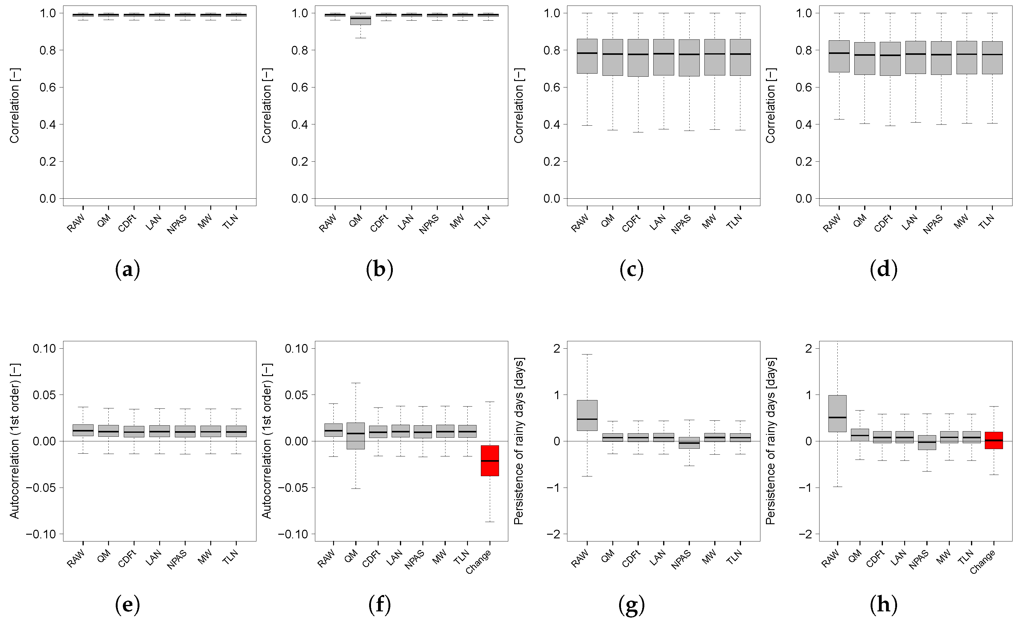
4.3. Evaluations of Temporal Properties

The boxplots in Figure 5 show the quality of the temporal properties of the two climate variables at each point in the domain over 1981–2010 and 2071–2100.

Let us examine the 1981–2010 period. For temperature, the correlations between the downscaled simulations and the references (Figure 5a) are greater than 0.95 and extremely similar for all experiments. Biases in terms of first-order autocorrelations (Figure 5e) also appear strongly equivalent for all experiments and very close to zero (∼0.01). For precipitation, the correlation between the downscaled simulations and the references (Figure 5c) is weaker than that for temperature, around 0.78 for the median value, without any significant differences between the experiments. This result is supplemented by the analysis of the persistence of precipitation (Figure 5g), whose biases are very close to zero for all the experiments, although the NPAS parameter can influence the results.

Over the 2071–2100 period, for temperature, the correlations (Figure 5b) remained satisfactory for all experiments (>0.95), although QM lagged behind the other experiments. Looking at biases in 1-day autocorrelations (Figure 5f), the values are, on average, equivalent for all experiments, but with a larger variability for QM. The findings for precipitation (Figure 5d,h) are almost identical to those over 1981–2010 (Figure 5c,g), with a median correlation of approximately 0.78 (Figure 5d) and a bias in persistence of precipitation (Figure 5h) close to zero. Again, this is clearly due to a change in persistence that is very close to zero, on average.

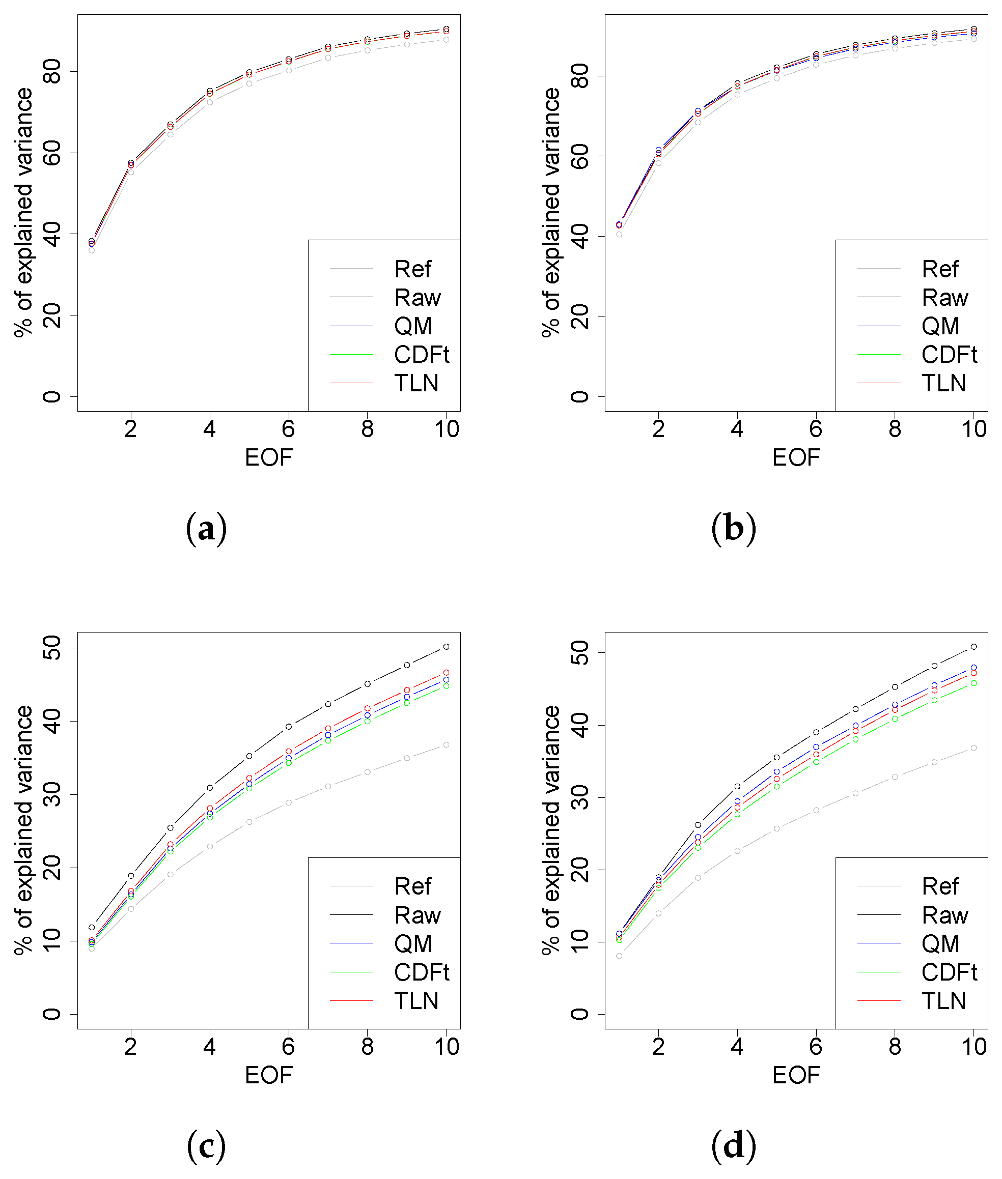
4.4. Multivariate Analysis: Inter-Variable & Spatial Properties

From now on, we focus only on the four experiments that are representative of the different behaviors seen previously: the raw, QM, CDF-t, and TLN experiments. Indeed, the results of the other variants are similar to those for CDF-t.

The correlation between the variables and spatial correlation is investigated in this section. In Figure 6, boxplots describe the variability of the biases in the correlations between temperature and precipitation.

The biases in the correlations are close to zero for all experiments over the calibration period (Figure 6a) and validation periods (Figure 6b). This indicates that the correlations between temperature and precipitation are similar between the reference model and each experiment, regardless of the projection time period. This was expected because a univariate quantile-based bias correction method, such as QM or the CDF-t variants, does not modify the inter-variable copula dependence function of the simulations to be adjusted, thus leaving the inter-variable correlations mostly untouched (see, e.g., [51]).

To investigate spatial variability, principal component analysis (PCA) was applied to each dataset and variable separately. Figure 7 shows the cumulative percentage of explained variance of the resulting Empirical Orthogonal Functions (EOFs) for the historical and future periods.

For temperature in the historical period (1981–2010, Figure 7a), all experiments show similar results, which are equivalent to those from the raw simulations. This was also expected because, as for the inter-variable correlation, univariate Quantile-Mapping-based methods do not correct the spatial dependence structure of the raw simulations, at least for continuous variables such as temperature. Hence, most of the spatial properties from the raw simulations are preserved by the QM and CDF-t experiments. As the cumulative percentage of explained variance of the raw simulations is a bit biased with respect to that of the reference simulations, all results reproduce this bias. The results for precipitation (Figure 7c) are somewhat different. Precipitation is a variable with a Dirac mass of zero. Applying a Quantile-Mapping-like method can modify the spatial dependence (spatial copula) of precipitation by modifying the probability of a dry time step. This explains the larger variability in the cumulative percentages of explained variance, as shown in Figure 7c. In general, improving the occurrence probability improves spatial properties, which is the case here. Indeed, all experiments tend to improve the raw simulations and are then closer to the reference. However, a clear remaining bias in the spatial properties with respect to the reference is visible. For the future period (2071–2100), the results (Figure 7b,d) are similar to those during the calibration period: the explained variance fractions are similar for all temperature experiments (Figure 7b), while for precipitation (Figure 7d), the explained variance fractions show some diversity among all experiments and are higher than those from the reference data.

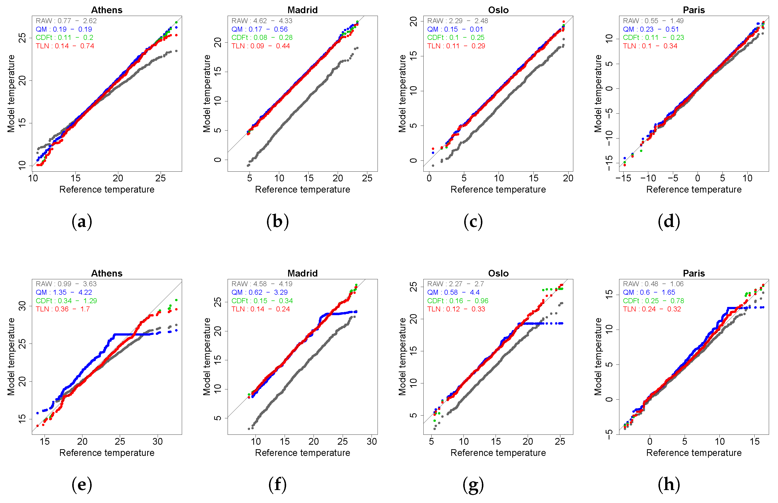
4.5. Evaluation at Local Scale

Here, we analyze the results at the grid point level to explore the performance at the local scale. We selected four cities spread over Europe—Athens, Madrid, Oslo, and Paris—and we now analyze the results of the experiments using quantile–quantile plots (QQplots) for 1981–2010 and 2071–2100 for temperature (Figure 8) and precipitation (Figure 9). Moreover, to compare these QQplots more quantitatively, the RMSE between the quantiles of the reference and the quantiles of the experiment has been computed (i) over the whole distribution, as well as (ii) over only the 10 highest values. The RMSE values are provided in the upper-left corner of each panel in Figure 8 and Figure 9.

For temperatures over 1981–2010 (Figure 8a–d), as expected, except for the raw simulations that show pronounced biases in distributions (especially for Madrid and Oslo), all the experiments provide satisfactory and relatively visually equivalent corrected distributions.

Focusing on 2071–2100, the temperature QQplot results (and the associated RMSE values) are now distinct (Figure 8e–h). For the four cities, the QM QQplots are now more distant from the diagonal line, meaning that the QM distribution is away from the reference distribution, even further away than the raw simulations for Athens. This is also visible in the RMSE values computed over the whole distribution. Moreover, the QM QQ-plots often display horizontally aligned (blue) dots in the right tail, indicating that QM fails to reproduce extreme temperatures. This limitation arises because the corrected values are capped by the maximum temperatures of the calibration period (e.g., Figure 8e with Athens). Visually, CDF-t and TLN display similar QQplots. However, the analysis of the RMSE values over the 10 highest values, although somewhat equivalent, gives a slight advantage to the TLN variant.

For precipitation over 1981–2010 (Figure 9a–d), the same conclusions as for temperature are obtained. Except for the raw simulations, all the experiments provide satisfactory and roughly equivalent QQplots. The main (although minor) differences appear in the tail of the distributions, for some extreme points. This is confirmed by the RMSE values that are relatively close for the whole distributions and more distinct over the 10 highest values.

Over 2071–2100 (Figure 9e–h), the precipitation distributions of the QM experiment are not as eccentric from those of the references as for the temperature (the RMSE values are smaller). However, the CDF-t and TLN experiments provide much better QQplots and RMSE values (both over the entire distribution and the 10 highest points).

5. Conclusions and Discussion

5.1. Conclusions

Because bias correction and downscaling methods are now commonly applied to climate simulations before running impact models, it is important to assess whether these methods are suitable in the context of climate change. Quantile Mapping (QM) is certainly the most widely used method because of its simplicity, ease, and speed of application. Therefore, this study investigated whether QM can provide robust future adjusted simulations in comparison with recent quantile-based variants that account for the climate change signal provided by the simulations to be corrected. To do so, a Perfect Model Experiment (PME) protocol was established. EURO-CORDEX temperature and precipitation simulations from the “Weather Research and Forecasting” (WRF) regional climate model (at 0.11° × 0.11° spatial resolution), forced by the IPSL global climate model, were used as pseudo-observations over the 1951–2100 period. These were upscaled to a coarse spatial resolution of 2° × 2°, and these large-scale simulations served as a proxy model data to be downscaled. Based on these pseudo-references and model proxies, the QM method, the “Cumulative Distribution Function-transform” (CDF-t) method, as well as four alternative parameterizations of the CDF-t approach (see Section 3.1 and Table 1) were calibrated over 1981–2010, applied over 1951–2100 (see Section 2.2), and evaluated (with respect to the pseudo-observations) over two periods: the calibration period (i.e., 1981–2010) and a far future period (2071–2100). Various metrics were used for the evaluations, and they were classified into different categories: marginal (i.e., univariate) properties, features of extremes, temporal properties, and multivariate properties (including spatial and inter-variable characteristics).

Comparing QM and CDF-t over the calibration period, both approaches improve the raw large-scale simulations, but they do not show much difference from each other regardless of the metrics used. This was expected because CDF-t, in its original configuration, is a generalization of QM. However, in the context of climate change, over the 2071–2100 period, major differences appeared depending on the metrics. In terms of marginal and extreme properties, while the CDF-t method and its various parameterizations provide close-to-zero biases, the QM method displays more pronounced biases. This indicates that QM partly fails to capture the climate change signal from the model data and propagate it to future projections. This is also visible at local scales when focusing on specific cities in Europe, where the statistical distributions from QM (both in precipitation and temperature) appear more biased than those from CDF-t. Therefore, Quantile Mapping is not recommended for the evolution of univariate distributions, basic marginal properties, and extreme properties.

Regarding CDF-t parameterizations, the value of the NPAS parameter can affect the quality of the results, particularly for precipitation. A low value (100, experiment “NPAS”) tends to increase the biases in the marginal and extreme precipitation properties, even over the calibration period. This is also true for extreme temperature properties, for which the NPAS experiment showed biases that were more pronounced than those of the other CDF-t variants. Moreover, to a much lesser extent, the choice of the double-moving-window length (MW experiment) can also induce biases. However, based on the different parameters chosen for the double-moving-window approach, the differences between MW and the CDF-t or TLN experiments remained very small.

When examining the multivariate (spatial and inter-variable) metrics, the different methods tested did not distinguish significantly from one another. This was expected because all the methods here are Quantile-Mapping-based approaches. By construction, such methods respect (i.e., reproduce) the time series of ranks from the model data to be adjusted, and the main dependence structures (i.e., spatial and/or inter-variable) and properties are mostly reproduced [51].

Generally, QM is inappropriate for adjustments in the context of climate change. Based on our evaluations, the approach illustrated by the TLN experiment is found to be the best approach for the routine application of the method [34,36]. Although the overall improvements remain modest, this approach acts as a safeguard for the tail of the distribution, ensuring better reliability in extreme value correction.

5.2. Discussion

Although this study provides new insights into the robustness of bias correction and downscaling methods, it can be further extended in different ways.

First, only one RCM driven by a single GCM was used to set up a perfect model experiment. If this were convenient for illustrating the proposed framework, a more robust evaluation would imply repeating the same procedure with other RCMs that are potentially driven by other GCMs. Indeed, this would allow for the testing of the statistical downscaling method of interest with various climate change signals and thus provide a more complete overview of the capability of the method to work in various changes.

Moreover, only univariate adjustment methods were tested. Recently, various multivariate bias correction (MBC) techniques have been developed to address spatial and/or inter-variable biases (e.g., [16,51,52]), as well as temporal biases (e.g., [53,54]). Such methods improve the credibility of multivariate adjustments [55], but more research is still needed to investigate their robustness in the context of climate change. A Perfect Model Experiment, similar to or inspired by the one proposed in the present study, adapted to multivariate methods could be of great relevance in that context.

The main drawback of the PME approach is that a model simulation is not a real observation for properly documenting distribution shifts under a warming trend. Reanalysis products could be used (e.g., from 1951 to present), but the magnitude of observed changes over the historical series is relatively small compared to the expected change by the end of the century and the corresponding potential shifts in distributions, particularly in the tails (i.e., extreme vents). However, the PME experiment is shown to be sufficient to test the ability of the “Stationarity assumption”, the ability of a method to reproduce the model warming trend of temperature, and the value at the end of the century (the “model sensitivity”).

In addition, as already mentioned in Section 2.1, by construction of our PME, the biases in the model data with respect to the references are only due to spatial smoothing because both datasets are the same but at different spatial resolutions. This has consequences for the type of atmospheric situations and events that our PME contains, which are not necessarily available when applying BC to (large-scale) GCM simulations in practice. Typically, GCMs currently struggle to accurately represent some storm types, particularly convective systems. By applying smoothing to high-resolution fields during the experimental setup, convective-scale or high-resolution-scale features are introduced that the original GCM could not simulate. This has important implications for interpreting the results and assessing the realism of the “perfect model” framework adopted in this study.

Recently, the bias adjustment of raw model projections with simple methods such as QM and even simpler ones based on mean and variance correction has been considered essential for evaluating extreme heat through threshold-based indicators, such as the number of warm days [56]. Here, we show that a simple QM model underestimates the warming signal and underperforms for all distribution moments (mean, extremes, etc.) when applied to daily projections. We argue that significant progress has been made in statistical downscaling/bias adjustment techniques [57] that offer robust alternatives, despite a higher computational cost, compared to simple methods that continue to be popular in the recent literature and should now be avoided.

References

1. Chokkavarapu, N.; Mandla, V.R. Comparative study of GCMs, RCMs, downscaling and hydrological models: A review toward future climate change impact estimation. SN Appl. Sci. 2019, 1, 1698. [Google Scholar] [CrossRef]
2. Müller, C.; Franke, J.; Jägermeyr, J.; Ruane, A.C.; Elliott, J.; Moyer, E.; Heinke, J.; Falloon, P.D.; Folberth, C.; Francois, L.; et al. Exploring uncertainties in global crop yield projections in a large ensemble of crop models and CMIP5 and CMIP6 climate scenarios. Environ. Res. Lett. 2021, 16, 034040. [Google Scholar] [CrossRef]
3. Laux, P.; Rötter, R.P.; Webber, H.; Dieng, D.; Rahimi, J.; Wei, J.; Faye, B.; Srivastava, A.K.; Bliefernicht, J.; Adeyeri, O.; et al. To bias correct or not to bias correct? An agricultural impact modelers’ perspective on regional climate model data. Agric. For. Meteorol. 2021, 304–305, 108406. [Google Scholar] [CrossRef]
4. Baron, C.; Sultan, B.; Balme, M.; Sarr, B.; Traore, S.; Lebel, T.; Janicot, S.; Dingkuhn, M. From GCM grid cell to agricultural plot: Scale issues affecting modelling of climate impact. Philos. Trans. R. Soc. B Biol. Sci. 2005, 360, 2095–2108. [Google Scholar] [CrossRef] [PubMed]
5. Challinor, A.J.; Osborne, T.; Morse, A.; Shaffrey, L.; Wheeler, T.; Weller, H.; Vidale, P.L. Methods and Resources for Climate Impacts Research. Bull. Am. Meteorol. Soc. 2009, 90, 836–848. [Google Scholar] [CrossRef]
6. Tapiador, F.J.; Navarro, A.; Moreno, R.; Sánchez, J.L.; García-Ortega, E. Regional climate models: 30 years of dynamical downscaling. Atmos. Res. 2020, 235, 104785. [Google Scholar] [CrossRef]
7. Maraun, D.; Widmann, M. Statistical Downscaling and Bias Correction for Climate Research; Cambridge University Press: Cambridge, UK, 2018. [Google Scholar] [CrossRef]
8. Maraun, D.; Wetterhall, F.; Ireson, A.M.; Chandler, R.E.; Kendon, E.J.; Widmann, M.; Brienen, S.; Rust, H.W.; Sauter, T.; Themeßl, M.; et al. Precipitation downscaling under climate change: Recent developments to bridge the gap between dynamical models and the end user. Rev. Geophys. 2010, 48, RG3003. [Google Scholar] [CrossRef]
9. Ayar, P.V.; Vrac, M.; Bastin, S.; Carreau, J.; Déqué, M.; Gallardo, C. Intercomparison of statistical and dynamical downscaling models under the EURO- and MED-CORDEX initiative framework: Present climate evaluations. Clim. Dyn. 2016, 46, 1301–1329. [Google Scholar] [CrossRef]
10. Gaitan, C.; Hsieh, W.; Cannon, A.; Gachon, P. Evaluation of Linear and Non-Linear Downscaling Methods in Terms of Daily Variability and Climate Indices: Surface Temperature in Southern Ontario and Quebec, Canada. Atmos.-Ocean 2014, 52, 211–221. [Google Scholar] [CrossRef]
11. Baño-Medina, J.; Manzanas, R.; Gutiérrez, J.M. Configuration and intercomparison of deep learning neural models for statistical downscaling. Geosci. Model Dev. 2020, 13, 2109–2124. [Google Scholar] [CrossRef]
12. Terzago, S.; Palazzi, E.; von Hardenberg, J. Stochastic downscaling of precipitation in complex orography: A simple method to reproduce a realistic fine-scale climatology. Nat. Hazards Earth Syst. Sci. 2018, 18, 2825–2840. [Google Scholar] [CrossRef]
13. Harris, L.; McRae, A.T.T.; Chantry, M.; Dueben, P.D.; Palmer, T.N. A Generative Deep Learning Approach to Stochastic Downscaling of Precipitation Forecasts. J. Adv. Model. Earth Syst. 2022, 14, e2022MS003120. [Google Scholar] [CrossRef]
14. Legasa, M.N.; Manzanas, R.; Calviño, A.; Gutiérrez, J.M. A Posteriori Random Forests for Stochastic Downscaling of Precipitation by Predicting Probability Distributions. Water Resour. Res. 2022, 58, e2021WR030272. [Google Scholar] [CrossRef]
15. Uytven, E.V.; Niel, J.D.; Willems, P. Uncovering the shortcomings of a weather typing method. Hydrol. Earth Syst. Sci. 2020, 24, 2671–2686. [Google Scholar] [CrossRef]
16. François, B.; Thao, S.; Vrac, M. Adjusting spatial dependence of climate model outputs with cycle-consistent adversarial networks. Clim. Dyn. 2021, 57, 3323–3353. [Google Scholar] [CrossRef]
17. Haddad, Z.S.; Rosenfeld, D. Optimality of empirical Z-R relations. Q. J. R. Meteorol. Soc. 1997, 123, 1283–1293. [Google Scholar] [CrossRef]
18. Déqué, M. Frequency of precipitation and temperature extremes over France in an anthropogenic scenario: Model results and statistical correction according to observed values. Glob. Planet. Change 2007, 57, 16–26. [Google Scholar] [CrossRef]
19. Gudmundsson, L.; Bremnes, J.B.; Haugen, J.E.; Engen-Skaugen, T. Technical Note: Downscaling RCM precipitation to the station scale using statistical transformations—A comparison of methods. Hydrol. Earth Syst. Sci. 2012, 16, 3383–3390. [Google Scholar] [CrossRef]
20. Galmarini, S.; Cannon, A.; Ceglar, A.; Christensen, O.; de Noblet-Ducoudré, N.; Dentener, F.; Doblas-Reyes, F.; Dosio, A.; Gutierrez, J.; Iturbide, M.; et al. Adjusting climate model bias for agricultural impact assessment: How to cut the mustard. Clim. Serv. 2019, 13, 65–69. [Google Scholar] [CrossRef]
21. Galmarini, S.; Solazzo, E.; Ferrise, R.; Srivastava, A.K.; Ahmed, M.; Asseng, S.; Cannon, A.; Dentener, F.; Sanctis, G.D.; Gaiser, T.; et al. Assessing the impact on crop modelling of multi- and uni-variate climate model bias adjustments. Agric. Syst. 2024, 215, 103846. [Google Scholar] [CrossRef]
22. Michelangeli, P.; Vrac, M.; Loukos, H. Probabilistic downscaling approaches: Application to wind cumulative distribution functions. Geophys. Res. Lett. 2009, 36, L11708. [Google Scholar] [CrossRef]
23. Vrac, M.; Drobinski, P.; Merlo, A.; Herrmann, M.; Lavaysse, C.; Li, L.; Somot, S. Dynamical and statistical downscaling of the French Mediterranean climate: Uncertainty assessment. Nat. Hazards Earth Syst. Sci. 2012, 12, 2769–2784. [Google Scholar] [CrossRef]
24. Kallache, M.; Vrac, M.; Naveau, P.; Michelangeli, P.A. Nonstationary probabilistic downscaling of extreme precipitation. J. Geophys. Res. 2011, 116, D05113. [Google Scholar] [CrossRef]
25. Vrac, M.; Noël, T.; Vautard, R. Bias correction of precipitation through Singularity Stochastic Removal: Because occurrences matter. J. Geophys. Res. Atmos. 2016, 121, 5237–5258. [Google Scholar] [CrossRef]
26. Oettli, P.; Sultan, B.; Baron, C.; Vrac, M. Are regional climate models relevant for crop yield prediction in West Africa? Environ. Res. Lett. 2011, 6, 014008. [Google Scholar] [CrossRef]
27. Colette, A.; Vautard, R.; Vrac, M. Regional climate downscaling with prior statistical correction of the global climate forcing. Geophys. Res. Lett. 2012, 39, L13707. [Google Scholar] [CrossRef]
28. Tisseuil, C.; Vrac, M.; Grenouillet, G.; Wade, A.; Gevrey, M.; Oberdorff, T.; Grodwohl, J.B.; Lek, S. Strengthening the link between climate, hydrological and species distribution modeling to assess the impacts of climate change on freshwater biodiversity. Sci. Total Environ. 2012, 424, 193–201. [Google Scholar] [CrossRef]
29. Tramblay, Y.; Neppel, L.; Carreau, J.; Sanchez-Gomez, E. Extreme value modelling of daily areal rainfall over Mediterranean catchments in a changing climate. Hydrol. Processes 2012, 26, 3934–3944. [Google Scholar] [CrossRef]
30. Defrance, D.; Ramstein, G.; Charbit, S.; Vrac, M.; Famien, A.M.; Sultan, B.; Swingedouw, D.; Dumas, C.; Gemenne, F.; Alvarez-Solas, J.; et al. Consequences of rapid ice sheet melting on the Sahelian population vulnerability. Proc. Natl. Acad. Sci. USA 2017, 114, 6533–6538. [Google Scholar] [CrossRef]
31. Defrance, D.; Sultan, B.; Castets, M.; Famien, A.M.; Baron, C. Impact of climate change in West Africa on cereal production per capita in 2050. Sustainability 2020, 12, 7585. [Google Scholar] [CrossRef]
32. Famien, A.M.; Janicot, S.; Ochou, A.D.; Vrac, M.; Defrance, D.; Sultan, B.; Noël, T. A bias-corrected CMIP5 dataset for Africa using the CDF-t method – a contribution to agricultural impact studies. Earth Syst. Dyn. 2018, 9, 313–338. [Google Scholar] [CrossRef]
33. Bartók, B.; Tobin, I.; Vautard, R.; Vrac, M.; Jin, X.; Levavasseur, G.; Denvil, S.; Dubus, L.; Parey, S.; Michelangeli, P.A.; et al. A climate projection dataset tailored for the European energy sector. Clim. Serv. 2019, 16, 100138. [Google Scholar] [CrossRef]
34. Noël, T.; Loukos, H.; Defrance, D.; Vrac, M.; Levavasseur, G. A high-resolution downscaled CMIP5 projections dataset of essential surface climate variables over the globe coherent with the ERA5 reanalysis for climate change impact assessments. Data Brief 2021, 35, 106900. [Google Scholar] [CrossRef] [PubMed]
35. Lanzante, J.R.; Nath, M.J.; Whitlock, C.E.; Dixon, K.W.; Adams-Smith, D. Evaluation and improvement of tail behaviour in the cumulative distribution function transform downscaling method. Int. J. Climatol. 2019, 39, 2449–2460. [Google Scholar] [CrossRef]
36. Noël, T.; Loukos, H.; Defrance, D.; Vrac, M.; Levavasseur, G. Extending the global high-resolution downscaled projections dataset to include CMIP6 projections at increased resolution coherent with the ERA5-Land reanalysis. Data Brief 2022, 45, 108669. [Google Scholar] [CrossRef] [PubMed]
37. Hersbach, H.; Bell, B.; Berrisford, P.; Hirahara, S.; Horányi, A.; Muñoz-Sabater, J.; Nicolas, J.; Peubey, C.; Radu, R.; Schepers, D.; et al. The ERA5 global reanalysis. Q. J. R. Meteorol. Soc. 2020, 146, 1999–2049. [Google Scholar] [CrossRef]
38. Muñoz-Sabater, J.; Dutra, E.; Agustí-Panareda, A.; Albergel, C.; Arduini, G.; Balsamo, G.; Boussetta, S.; Choulga, M.; Harrigan, S.; Hersbach, H.; et al. ERA5-Land: A state-of-the-art global reanalysis dataset for land applications. Earth Syst. Sci. Data 2021, 13, 4349–4383. [Google Scholar] [CrossRef]
39. Themeßl, M.J.; Gobiet, A.; Heinrich, G. Empirical-statistical downscaling and error correction of regional climate models and its impact on the climate change signal. Clim. Change 2012, 112, 449–468. [Google Scholar] [CrossRef]
40. de Ela, R.; Laprise, R.; Denis, B. Forecasting Skill Limits of Nested, Limited-Area Models: A Perfect-Model Approach. Mon. Weather Rev. 2002, 130, 2006–2023. [Google Scholar] [CrossRef]
41. Vrac, M.; Marbaix, P.; Paillard, D.; Naveau, P. Non-linear statistical downscaling of present and LGM precipitation and temperatures over Europe. Clim. Past 2007, 3, 669–682. [Google Scholar] [CrossRef]
42. Dixon, K.W.; Lanzante, J.R.; Nath, M.J.; Hayhoe, K.; Stoner, A.; Radhakrishnan, A.; Balaji, V.; Gaitán, C.F. Evaluating the stationarity assumption in statistically downscaled climate projections: Is past performance an indicator of future results? Clim. Change 2016, 135, 395–408. [Google Scholar] [CrossRef]
43. Chen, F.; Gao, Y.; Wang, Y.; Li, X. A downscaling-merging method for high-resolution daily precipitation estimation. J. Hydrol. 2020, 581, 124414. [Google Scholar] [CrossRef]
44. Jacob, D.; Petersen, J.; Eggert, B.; Alias, A.; Christensen, O.B.; Bouwer, L.M.; Braun, A.; Colette, A.; Déqué, M.; Georgievski, G.; et al. EURO-CORDEX: New high-resolution climate change projections for European impact research. Reg. Environ. Change 2014, 14, 563–578. [Google Scholar] [CrossRef]
45. Taylor, K.E.; Stouffer, R.J.; Meehl, G.A. An Overview of CMIP5 and the Experiment Design. Bull. Am. Meteorol. Soc. 2012, 93, 485–498. [Google Scholar] [CrossRef]
46. Jones, C.; Giorgi, F.; Asrar, G. The coordinated regional downscaling experiment (CORDEX). An international downscaling link to CMIP5. CLIVAR Exch. 2011, 56, 1797680. [Google Scholar]
47. Dufresne, J.L.; Foujols, M.A.; Denvil, S.; Caubel, A.; Marti, O.; Aumont, O.; Balkanski, Y.; Bekki, S.; Bellenger, H.; Benshila, R.; et al. Climate change projections using the IPSL-CM5 Earth System Model: From CMIP3 to CMIP5. Clim. Dyn. 2013, 40, 2123–2165. [Google Scholar] [CrossRef]
48. Schulzweida, U. CDO User Guide (2.3.0). Zenodo 2023. [Google Scholar] [CrossRef]
49. Vrac, M.; Vaittinada Ayar, P. Influence of Bias Correcting Predictors on Statistical Downscaling Models. J. Appl. Meteorol. Climatol. 2017, 56, 5–26. [Google Scholar] [CrossRef]
50. Maraun, D.; Widmann, M.; Gutiérrez, J.M.; Kotlarski, S.; Chandler, R.E.; Hertig, E.; Wibig, J.; Huth, R.; Wilcke, R.A. VALUE: A framework to validate downscaling approaches for climate change studies. Earth’s Future 2015, 3, 1–14. [Google Scholar] [CrossRef]
51. Vrac, M. Multivariate bias adjustment of high-dimensional climate simulations: The Rank Resampling for Distributions and Dependences (R2 D2) bias correction. Hydrol. Earth Syst. Sci. 2018, 22, 3175–3196. [Google Scholar] [CrossRef]
52. Cannon, A.J. Multivariate Bias Correction of Climate Model Output: Matching Marginal Distributions and Intervariable Dependence Structure. J. Clim. 2016, 29, 7045–7064. [Google Scholar] [CrossRef]
53. Vrac, M.; Thao, S. R2 D2 v2.0: Accounting for temporal dependences in multivariate bias correction via analogue rank resampling. Geosci. Model Dev. 2020, 13, 5367–5387. [Google Scholar] [CrossRef]
54. Robin, Y.; Vrac, M. Is time a variable like the others in multivariate statistical downscaling and bias correction? Earth Syst. Dyn. 2021, 12, 1253–1273. [Google Scholar] [CrossRef]
55. François, B.; Vrac, M.; Cannon, A.J.; Robin, Y.; Allard, D. Multivariate bias corrections of climate simulations: Which benefits for which losses? Earth Syst. Dyn. 2020, 11, 537–562. [Google Scholar] [CrossRef]
56. Iturbide, M.; Casanueva, A.; Bedia, J.; Herrera, S.; Milovac, J.; Gutiérrez, J.M. On the need of bias adjustment for more plausible climate change projections of extreme heat. Atmos. Sci. Lett. 2022, 23, e1072. [Google Scholar] [CrossRef]
57. Abdelmoaty, H.M.; Rajulapati, C.R.; Nerantzaki, S.D.; Papalexiou, S.M. Bias-corrected high-resolution temperature and precipitation projections for Canada. Sci. Data 2025, 12, 191. [Google Scholar] [CrossRef] [PubMed]
Figure 1. Illustration of the double-moving-window approach for continuous statistical downscaling. The calibration period is fixed at 1981–2010. For projections, a (external) window of 20 years is used to fit the distributions required to apply CDF-t, while another 10-year (internal) window is used at the center of the time window to perform downscaling. The same procedure is then repeated after advancing both windows by 10 years.
Climate 13 00137 g001
Figure 2. Illustration of the LAN procedure. Left panel: A quantile–quantile (QQ) plot of the October temperature over the period 2086–2100 for the grid cell covering Paris, comparing reference data with raw simulations (gray crosses), CDFt-corrected data (black crosses), and LAN-corrected data (blue crosses). Right panel: Zoom on the upper tail, highlighting the LAN correction; the last TLN values (here, 5 points) are adjusted using the correction Δ , defined as the average difference over the preceding NPT points (here, 10). Points used to compute Δ are circled in red.
Climate 13 00137 g002
Figure 3. Boxplots of biases for the raw simulations and six experiments in abscissa in the marginal distributions of the October temperature over the calibration period (1981–2010) (first column, panels (a,e)) and the future period (2071–2100) (second column, panels (b,f)) and for precipitation over the calibration period (1981–2010) (third column, panels (c,g,i)) and the future period (2071–2100) (last column, panels (d,h,j)). Biases in mean (ad) and standard deviation (eh) for both temperature and precipitation and biases in the number of rainy days (i.e., >1 mm/day, panels (i,j)). The boxplots display the spatial variability of the biases. In the future period panels, the red boxplot indicates the change from the historical period to the future one for each indicator.
Climate 13 00137 g003
Figure 4. Boxplots of biases for the raw simulations and six experiments in abscissa in the extremes of the October temperature over the calibration period (1981–2010) (first column, panels (a,e,i)) and the future period (2071–2100) (second column, panels (b,f,j)) and for precipitation over the calibration period (1981–2010) (third column, panels (c,g,k)) and the future period (2071–2100) (last column, panels (d,h,l)). Biases in Q98 for both variables (ad) in the number of warm days (e,f), in the Q02 of temperature (i,f), in the number of very heavy wet days (g,h), and in the Q02 of >1 mm/day precipitation (k,l). As in Figure 3, in the future period panels, the red boxplot indicates the change from the historical period to the future one for each indicator.
Climate 13 00137 g004
Figure 5. Boxplots of statistics or biases for the raw simulations and six experiments in abscissa in the temporal properties of the October temperature over the calibration period (1981–2010) (first column, panels (a,e)) and the future period (2071–2100) (second column, panels (b,f)) and for precipitation over the calibration period (1981–2010) (third column, panels (c,g)) and the future period (2071–2100) (last column, panels (d,h)). Pearson correlations of the downscaled simulations and the references (ad), biases in lag 1-day auto-correlation of temperature (e,f), and biases in mean persistence of precipitation (g,h).
Climate 13 00137 g005
Figure 6. Boxplots of biases for the raw simulations and three experiments in abscissa in Pearson’s correlation between temperature and precipitation per grid point in October: (a) biases over the historical period (1981–2010) and (b) over the future period (2071–2100). The red box corresponds to the change between future and historical.
Climate 13 00137 g006
Figure 7. Cumulative percentages of the explained variance in the first ten Empirical Orthogonal Functions (EOFs) for temperature and precipitation over the calibration (1981–2010) and future periods (2071–2100) in October. The EOFs are obtained from PCAs performed from matrices composed by each grid cell as a variable (column) and each day as a realization (line) for each dataset or experiment: (a) temperature over the calibration period, (b) temperature over the future period, (c) precipitation over the calibration period, and (d) precipitation over the future period.
Climate 13 00137 g007
Figure 8. Quantile–quantile plots (QQplots) of reference versus downscaled data in October for the temperature over the calibration period (1981–2010, top row, Figures (ad)) and over the projection period (2071–2100, bottom row, Figures (eh)) over 4 cities—(a,e) Athens, (b,f) Madrid, (c,g) Oslo, and (d,h) Paris) for three experiments (colored dots), QM (black), CDFt (green), and TLN (Red), as well as for the raw simulations (grey). In order to quantify the quality of the QQplots in general as well as for the extremes, in the upper-left corner of each panel, for each experiment, the value of the RMSE between the quantiles of the reference and the quantiles of the experiment is given when computed on the whole distribution, followed by the value of the same RMSE but computed only on the 10 highest values.
Climate 13 00137 g008
Figure 9. Same as Figure 8 but for precipitation.
Climate 13 00137 g009