Recovery and Reconstructions of 18th Century Precipitation Records in Italy: Problems and Analyses

Abstract

Precipitation is one of the main meteorological variables in climate research and long records provide a unique, long-term knowledge of climatic variability and extreme events. Moreover, they are a prerequisite for climate modeling and reanalyses. Like all meteorological observations, in the early period, every observer used a personal measuring protocol. Instruments and their locations were not standardized and not always specified in the observer’s metadata. The situation began to change in 1873 with the foundation of the International Meteorological Committee, though the complete standardization of protocols, instruments, and exposure was reached in 1950 with the World Meteorological Organization. The aim of this paper is to present and discuss the methodology needed to recover and reconstruct early precipitation records and to provide high-quality dataset of precipitation usable for climate studies. The main issues that have to be addresses are described and critically analyzed based on the longest Italian precipitation series to which the methodology was successfully applied.

1. Introduction

Measurements of precipitation frequency, amount, and duration are fundamental in climatological and hydrological studies. Global inventories of climate datasets are used for monitoring precipitation variation over time, for investigating extreme events, and for understanding the mechanisms involved (e.g., [1,2]). Moreover, precipitation datasets can help to understand the occurrences of other kind of extreme events, such as cyclones [3].

The longer the precipitation time series, the better our knowledge of the past, trends and variability. A prerequisite is that meteorological records are homogeneous over time. However, in the 18th century, and for much of the 19th century, observers used different and not standardized instruments and took readings without common protocols.

Only after the foundation of the International Meteorological Committee (IMC) in 1873 [4,5] were common protocols and practices for weather observations established, and precise indications for instrument exposure, elevation, and sampling were provided. The instrument standardization has led to the need for new studies and shared agreements [6,7,8]. Data became fully homogeneous after the creation of the World Meteorological Organization (WMO) in 1950. WMO established the Commission for Instruments and Methods of Observation (CIMO), whose mission is to promote and facilitate international standardization, which implied the compatibility of the instruments and the observation methods used by Members, including the definition of precipitation, the instrument characteristics, its position, and the reading times.

This means that the observations taken after 1950 follow the WMO norms. Those taken between 1873 and 1949 are gradually aligning, as the ideas and criteria were being defined. Those taken before are completely independent. This fact constitutes a serious difficulty when someone wants to join early records with modern ones to obtain long time series, to establish trends or to determine whether there have been climate changes.

The definition of precipitation influences both amount and frequency and has changed over the years: in the 18th and 19th centuries, precipitation included “any form of water falling from the sky, i.e., rain, snow, hail, dew, fog or any other type” [9], while the current definition of the WMO excludes any type of atmospheric condensation [8]. The total amount of precipitation reaching the ground is measured as the vertical depth of water and recorded as the linear depth in millimeters (collected volume/catchment area), or $\mathrm{kg}/{\mathrm{m}}^2$ (collected mass/catchment area). In the past, it was also measured in terms of weight per unit surface. Today, the minimum daily amount of precipitation is established to be 0.1 mm; lower values are referred to as traces, and the corresponding day should not be considered rainy [8]. In the past, even values below this threshold were considered.

In the 18th century, the rain gauge was generally a cylinder with a funnel provided of a convenient rim and a collecting vessel [8]. The small, square, unheated funnels were only suitable for collecting rain, as the hailstones were bounced out, and snow was either blown away by the wind or accumulated, obstructing the funnel. To measure snow, the observers were forced to take from the ground a sample with a section equal to the funnel and melt it. When they understood that the ratio of the snow depth to water was 10:1 [8], it was sufficient to measure the snow depth with a graduated rod. Therefore, the instruments could only measure liquid precipitation and snow depth was separately measured and reported in old registers.

Precipitation measurement is particularly sensitive to exposure, wind, and topography, so the instrument location and elevation are critical. WMO specifies that the elevation of funnel orifices should be between 0.5 and 1.5 m above the ground [7,8]. In addition, “the distance of any obstacle should not be less than twice the height of the object above the rim of the gauge, and preferably four times the height” [8]. Funnels placed at different elevation from the ground measure different amounts [7,10,11]. In general, the best location should be in open sites, far from buildings, trees, and any other obstacles. However, in the 18th and 19th centuries the rain gauges were exposed on roofs, to have an unobstructed horizon.

In Italy, the earliest instrumental precipitation records started at the beginning of the 18th century, before the standardizations of IMC. However, there is another problem besides the lack of standardization: logs generally did not include metadata, and, in addition, most original logs were dispersed or lost. Scholars were interested in improving instruments, taking measurements, seeking relationships between variables and Moon’s phases, public health, agriculture, and so on. It was expensive to publish drawings, which were limited to the essential. As a matter of fact, the original sources report a lot of data and theoretical discussions, but poor explicit information about instruments, as well as their elevation and exposure. The lack of metadata constitutes a serious problem to interpret and correct data. Our knowledge has been derived from the relationships between scholars, who adopted same or similar solutions, the recommendations of the first international network, or contemporary colleagues living in other places.

This paper addresses the issue of the recovery and reconstruction of 18th century precipitation series with a combined historical and physical approach. When dealing with early meteorological series, it is necessary to place them in their historical context, since the problems to be solved are closely linked to the period under examination and to the measuring practices of that time. The final aim is to provide a comprehensive methodology to obtain a sound series to be used in climate studies. The longest Italian series starting in the 18th century that have been already recovered are the ideal playing field to demonstrate the application of this methodology.

The paper is structured as follows. The general methodology is presented in Section 2, as well as the instruments used in the past, the description of which is essential to understand the main problems, and their solution. Section 3 explains the main biases and their effect on rain characteristics, and provides methods for data correction. Section 4 illustrates how to join subseries and check the reliability of the obtained long series. Conclusions are finally drawn in Section 5.

2. Materials and Methods

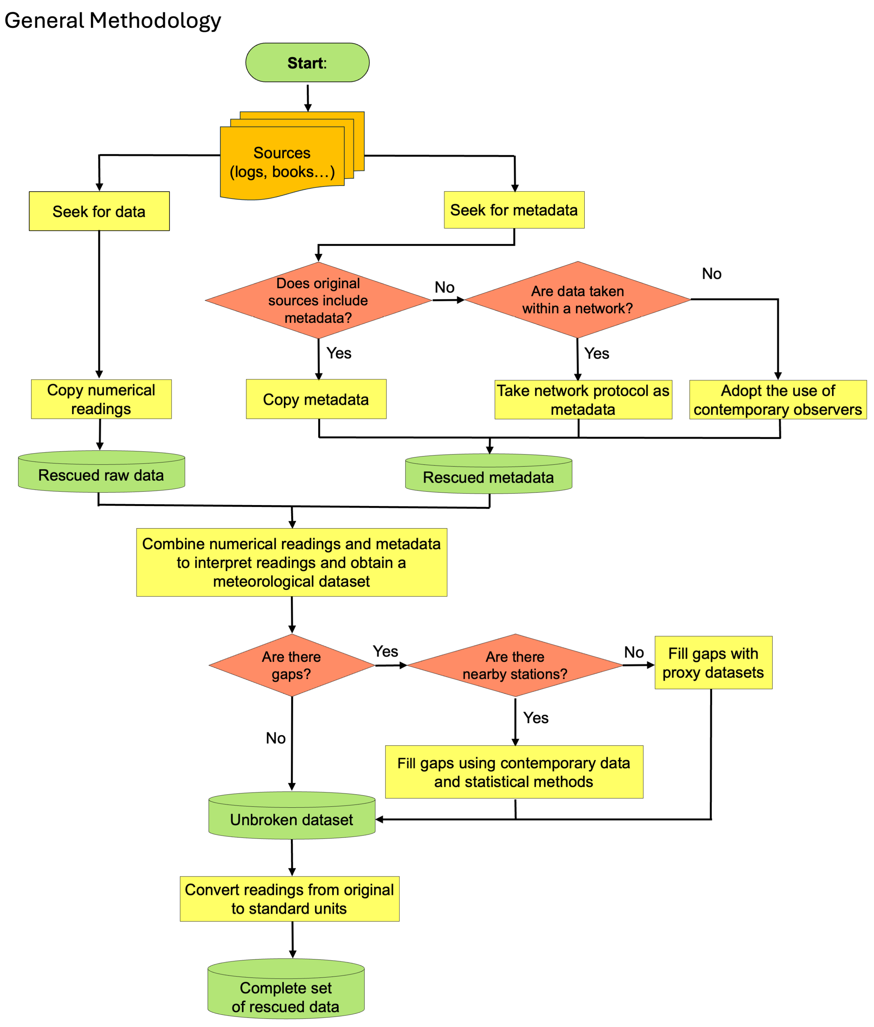
2.1. Methodology

The methodology to recover and reconstruct a long time series of precipitation develops through three main stages, illustrated in Figure 1, Figure 2 and Figure 3. The first stage consists of the recovery of precipitation data and metadata (i.e., information concerning observers, instruments, locations, observing time, etc.) (Figure 1). Metadata are crucial to convert data from original to standard units, and thus, to obtain a complete dataset. Moreover, metadata are fundamental to proceed with the second stage, i.e., to evaluate and correct some general bias, independent by the rain gauge, as the identification of dew, the exposure of the funnel, the sampling time (Figure 2). Unfortunately, in most cases, no information was given or found, and therefore, metadata should be recovered collecting information from other sources (Figure 1). In the 18th century, some meteorological network flourished and established common observation protocols. In other cases, observers used procedures and instruments like those used by leading scientists. This preliminary investigation is fundamental to gather information that will be used in the next stages. Finally, the third stage is focused on rain gauge dependent biases, which, once resolved, allowed the subseries to be merged in a long series (Figure 3). At this step, it is fundamental to check for data homogeneity to avoid introducing changes not related to climate (Figure 3).

WMO specifies that “A quality control system should include procedures for tracing the observations to their source to verify them and to prevent the recurrence of errors. Quality control is applied in real time, but it also operates in non-real time, as delayed quality control” [12]. In addition, the standard quality tests involve the comparison of the data of more stations [13] and cannot be applied to single datasets. The methodology presented in this paper has been specifically developed for early precipitation series, which have characteristics and issues different from modern ones, and thus, do not have the standard characteristics that allow for the use of WMO data quality control system. Nevertheless, the procedures described in this paper allow to analyze critically the source of the data taken before the WMO regulations were established and to identify the possible source of errors, so it might be considered as a validation procedure of early data, that, if followed, allow to obtain a sound long series starting in the early instrumental period.

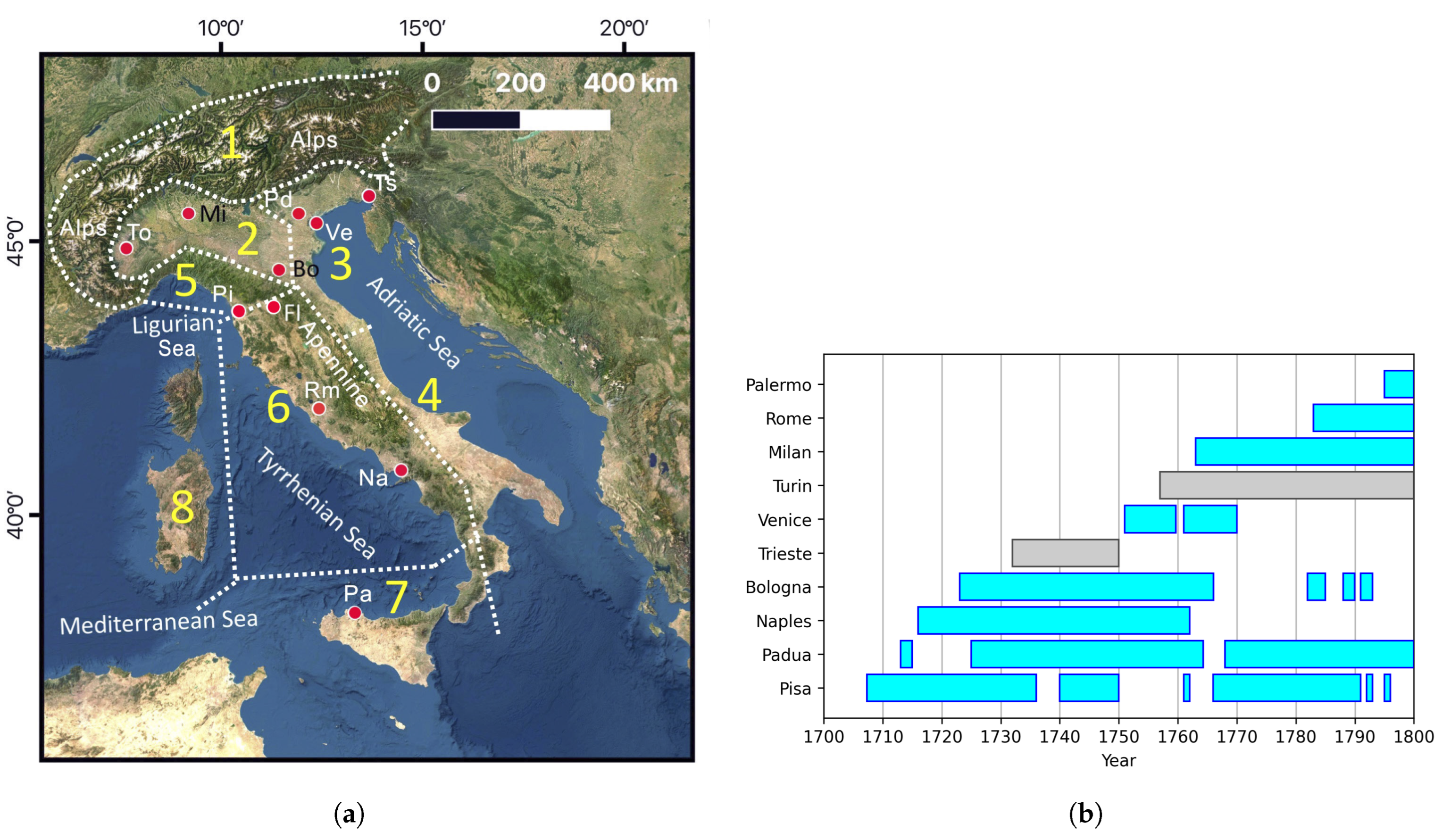
2.2. Overview of the Earliest Italian Precipitation Series

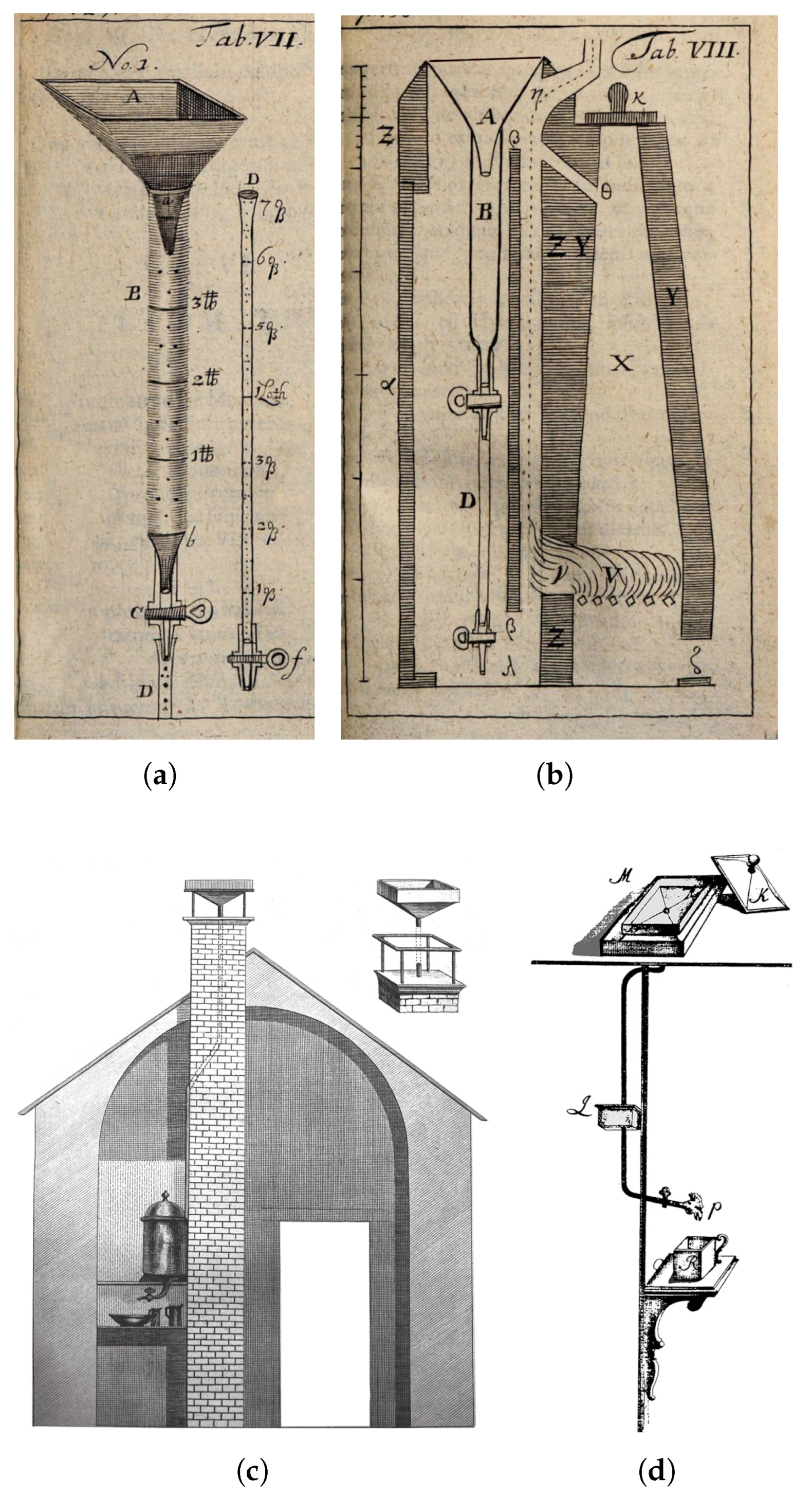
In Italy, the 18th century began without meteorological observations, but during this century, some people started to make measurements. These people were distributed over the whole Italian peninsula (Figure 4a). Some of these series have already been recovered (e.g., Padua, Pisa, Milan), while for some others (e.g., Bologna, Rome, Palermo), rescuing (recovery and correction) is underway. However, these records are hardly comparable, due to the complex geographic features of Italy. Italy is a thin and long peninsula, with the Alps and the Apennine Mountain chains, facing different seas on the east and west. The result is that the territory is not climatically homogeneous and is divided in eight climate regions, as shown in Figure 4a [14], as follows: Region 1: Alps; Region 2: Po Valley; Region 3: Northern Adriatic coast; Region 4: Central and Southern Adriatic coast; Region 5: Ligurian coast; Region 6: Tyrrhenian coast; Region 7: Calabria and Sicily; Region 8: Sardinia. The Alps have a cold climate; Po Valley is continental; climate regions in northern and central Italy have a precipitation regime for the whole year, but with maxima in spring and autumn due to the penetration of Atlantic disturbances and rare showers in summer due to thermo-convective activity; regions in southern Italy have a rainy cold season and arid warm season; the western coast is more exposed to westerly winds and the Atlantic disturbances, while the eastern coast is more exposed to northern and eastern winds. As a result, sites even with short distances between them, but separated by mountain chains or belonging to different climate regions, may have different precipitation regimes. This makes it difficult to compare between different sites and to fill in data gaps using neighboring stations. This drawback is particularly relevant in the 18th century and in the first half of the 19th century, when the observations available were few, and in general belonging to different climate regions.

An overview of the main series started in the 18th century in Italy is shown in Figure 4b. Several series started in the 19th century, and especially after 1860, when Italy was unified in a single kingdom, and all the services were reorganized, including the meteorological observations. Some of these series were recovered and reconstructed using the methods described in this paper, and their data has been used to illustrate the methodologies used. They are briefly presented in Appendix A.

2.3. Instruments

In the 18th century, rain gauges were hand crafted, especially funnels. They were square shaped, to have a known section, and with the rim they seemed cubic boxes with open top. Conical funnels with cylindrical rim required technical improvements and became popular in the second half of the 19th century, thanks to industrial production.

Precipitation amount could be measured using three different systems, i.e., by weight with a balance, by volume using cups of known capacity, and by depth, dipping a graduated rod inside the collecting vessel [9]. Amounts were usually expressed in local units.

Nowadays, with the introduction of the metric system, the value of the density of water is $1\mathrm{g}/{\mathrm{cm}}^3$. In this manner, an amount of water collected in a vessel with unit cross section, ($1{\mathrm{cm}}^2$), has a weight of A grams, a volume of $A{\mathrm{cm}}^3$, and a depth of A cm. So, a certain quantity of water, measured in terms of weight, volume, and depth, has the same numerical value (although with different dimensional units) and the choice of the physical quantity is irrelevant. However, when physical quantities were measured in units not simply related between each other, the results were different. Now, surface and volume units are defined as the second and third power of the unit of length, respectively, but before the adoption of the metric system, this was not so simple, because length, surface area, and volume were not multiples of each other. For instance, in Venice, the basic unit of length was the $\mathrm{foot}=34.775\mathrm{cm}$; a $\mathrm{cubic}\mathrm{foot}=0.42048{\mathrm{m}}^3$; the unit of volume was the $\mathrm{tub}=85.8480\mathrm{L}$; and the unit of weight was the $\mathrm{libra}=301.230\mathrm{g}$, which was divided in 12 ounces.

In addition, depending on the unit, location, and period, the subunits followed different ratios, e.g., $1/12$, $1/10$, $1/8$, and $1/4$. This makes the transformations from one unit into another and the conversion of the values to the metric system very complex. Therefore, the precipitation was expressed in the local unit related to the measuring system, i.e., weight, volume, or depth. Sometimes, but rarely, observers calculated a personal conversion table and published their readings in two columns with distinct units, e.g., one by weight and one by depth [15].

For instance, in Pisa, Michel Angelo Tilli, Carlo Rinaldini, Angelo Attilio Tilli, and Gian Lorenzo Tilli measured by weight [16,17]. They operated in an Institute of Botany and had precise balances. An advantage of the weighing method (except when the funnel is on the top of a chimney, like in Pisa) is that there is no difference between rain, snow, and hail.

Toaldo in Padua [9,18,19] and Beccari in Bologna [20] measured by volume. This operation was very easy with the help of calibrated cups. Toaldo used three cubic cups with capacity 1, 4, and 27 cubic Paris inches, i.e., 7.33, 29.31, and $197.84{\mathrm{cm}}^3$, respectively. In case of snow, it was necessary to melt ice.

Poleni in Padua [18,19] and Temanza and Pollaroli in Venice [21] measured by depth. Depth could be magnified in proportion to the ratio between the cross sections of the funnel and the storage can, or the square of their diameters. Jurin recommended a $1/10$ ratio for the funnel/storage can diameters, which allows $1/100$ magnification in depth [22].

Poleni kept the funnel on the top of a chimney of their roof, dragged the rainwater with a metal pipe, and collected it in a closed reservoir located in a room below. This method was later recommended by Hemmer [23] and Cotte [24] (Figure 5a).

Hemmer [23] was clear about the instrument location. The funnel had a square section, was located on the roof, and a drainage pipe transported the water in a room, where it was collected in a reservoir. Practically, Hemmer formalized the practice established with the Jurin’s network. The drawing contained an additional instruction, i.e., the funnel could be covered with a lid, perhaps to prevent evaporation or the entry of leaves during the dry periods between one rainfall and another. Obviously, putting the funnel on and off between rainfalls had to have been quite a hassle, and to our knowledge, no one adopted this practice (Figure 5d).

The chimney location was popular for some claimed advantages, i.e., unobstructed horizon, reading the amounts without going outside under the rain, almost no evaporation, and the possibility of melting the snow with a gentle fire on the fireplace. The use of chimneys was never mentioned by Poleni, but was clearly explained by their contemporary Leutmann [25] who lived in Wittenberg, Germany.

Leutmann [25] gave precise details concerning the instruments, their exposure, and their operation. The rain gauge (Figure 5b) constituted a funnel A with a square opening, and the neck was fixed inside a big collecting vessel B with 4 libra capacity (1 libra $\approx 322$–329 g), with a graduation in weight (i.e., libra and half uncia, i.e., $1/32$ libra, called Loth, 1 Loth $\approx 10$ g), and a faucet C on the bottom. It was possible to drain the collected water into another similar phial D, but thinner and with fine graduation in Loth and fractions of Loth, (i.e., $1/4$ Loth and $1/40$ Loth). This ensured a precise evaluation of the weight, or the volume, of the rainwater. The rain gauge, i.e., the funnel with the two phials, was inserted on the top of a chimney (Figure 5c). The chimney acted as a frame to hold the instrument but was very effective in shielding it from the solar radiation, avoiding evaporation losses. Leutmann lived in a cold climate region and the problem of snow was relevant. He decided to add a furnace X, with communication ducts with the chimney holding the instrument, so that the hot air from the flame V or the smoke $\theta$ could melt the snow in the funnel and keep it above the freezing point. This condition was crucial for the collecting vessels made of glass, which could be broken by ice. Within the chimney, a panel $\beta$ separated the glasswork from the flame and the hot air to avoid damage or evaporation.

Poleni [26] suggested to apply the principle of communicating vessels and proposed to connect a vertical graduated glass tube externally to the storage can, so that one could read the water depth at any instant. However, he never applied this method. Burnings, based on Poleni’s idea [26], realized a prototype in the Netherlands (Figure 6a) [27] that became an example for several instrument makers in the 19th century, as it made the readings easier. However, it implied no magnification, capillary meniscus distortion, and some undetected stagnant water under the connection between the can and the tube (Figure 6b) that increased the threshold [28].

The tipping bucket rain gauge (Figure 6c,d) was invented in the 1660s by Christopher Wren and Robert Hooke but arrived two centuries later in Italy. It constituted a twin pair of compartments, mounted on a spindle in the middle. The two compartments were symmetrically disposed, so that the bucket was balanced in unstable equilibrium about a horizontal axis. Rain flowing out of the funnel fell into the uppermost compartment and when it had filled it, the center of gravity was displaced and the bucket overbalanced, tipped, and emptied the precipitation. A mechanical counter recorded the number of tips. The collecting volume of the compartments determined threshold, resolution, and amount of water that could remain undetected in the bucket. This latter could be significant for light rainfalls that might remain below the threshold. This bias has high impact on the frequency, because light rainfalls are the most frequent ones, but has a minor impact on the total amount. In the case of intense showers, the water fallen during the pivoting movement is lost. This bias reduces the total amount of collected water, underestimating the extreme events [28]. During the 18th and 19th centuries, the shape of funnels changed, from squared (Figure 6a) to circular (Figure 6g).

The siphon rain gauge (Figure 6e) was invented by Gustav Hellmann in 1897, and was improved in 1910 by Luigi Palazzo, Director of the Central Office of Meteorology and Geodynamics, Rome. When the national Weather Service was established in Italy, this instrument was adopted by all Meteorological Observatories. It is affected by the same biases mentioned for the tipping bucket, but of a different magnitude. Another rain gauge used in Italy was the agrario (i.e., agrarian), a simple vessel with an opening funnel on the top and a tap on the bottom. The amount of water was measured with calibrated boxes (Figure 6f).

Detailed reviews of thresholds and drawbacks of rain gauges used from the 18th to the 20th centuries have been made elsewhere [20,21,28]).

3. Main Biases Affecting Precipitation Series and Their Solution

3.1. Gaps and Missing Data

Almost all long instrumental series are affected by gaps, especially in the early period. At the beginning, data were collected by a single observer, so sudden interruptions could occur for different reasons: instruments malfunctions, relocation, poor health or even death of the observer, political changes, wars, and so on. Recovering or reconstructing missing precipitation records means to complete both frequency and amount.

Various approaches have been developed to estimate missing values in precipitation series. The most successful methods to fill or validate a dataset of modern data involve the availability of neighboring contemporary stations. Several statistical techniques can be used for this aim at different level of complexity. There is no single gap-filling method, as it depends on the specific case [32,33]. Some factors influence the choice: the percentage of missing data and the length of gaps [34]; the correlation between involved stations [33]; and the homogeneity of measuring protocols, i.e., instrument, exposure, location, and time of observation. The distance from the target station is less important than the correlation between stations [33]. According to Bellido-Jiménez et al. [35], the use of neighboring stations is more efficient than the autocorrelation, i.e., the use of past (or future) data of the target station itself.

This approach can be hardly applied to early series, because in that period, there were only a few stations, mostly distributed in regions with different climates. In addition, the observational procedures were not standardized, making difficult any comparison between observers. In a few cases, the presence of a sufficient number of stations allowed to extend and integrated instrumental series at least from the 19th century onward [36].

In the past, some scientists looked for monthly relationships between amounts and number of rainy days [9,37,38], but with unsatisfactory results.

Other methods transformed documentary sources into numerical values using the available data as calibration. Several scales of indices were developed and used as proxy in different area and time periods, both to reconstruct past climate when measurements were not available and to increase the spatial resolution when there were a few stations [39,40,41,42,43,44,45,46,47]. In Italy, Diodato [48] used documentary sources to estimate precipitation in Sicily since 1675. Raicich [49] reconstructed precipitation frequency in Trieste for 18 years of 17th century. Camuffo et al. [21], using qualitative descriptions of contemporary observers, recovered the 1764–1767 gap of the Padua precipitation. Generally, the time scale of the reconstruction was monthly, seasonally, or yearly. Rarely, the proxy methods reached a daily resolution: Ge et al. [45] made a proxy using daily quantitative description, but reconstructed the precipitation series at monthly resolution. Dominguez-Castro et al. [40] and Camuffo et al. [21] reached the daily resolution. The best-ever technique for daily precipitation reconstruction in early series cannot be assessed, as it is strongly dependent on the quality and quantity of data and metadata available, so every case needs to be considered individually.

3.2. Missing Original Logs

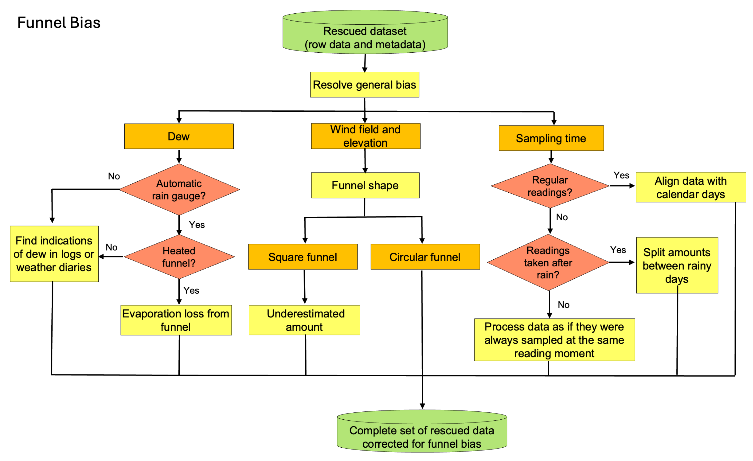
In case the original logs were lost, it is possible to fill gaps using the methods described in Section 3.1 or trying to recover the original data from some other sources: when scientists joined to national or international networks, they used to send them a copy of their measurements. Sometimes, scientists also published their data in literary journals or ephemerides magazines.

Data of the early series of Pisa and Naples were found in the publications of the network organized by William Derham [50,51]. Poleni in Padua and Taglini in Pisa joined the network of the Royal Society [22] and published some data in the Philosophical Transactions. Later, Toaldo and Chiminello in Padua, Matteucci in Bologna, and Calandrelli in Rome joined the network organized by Hemmer [23,52] and sent them their data to be published in the Ephemerides Societatis Meteorologicae Palatinae.

The type and time resolution of these observations changed at every publication: in certain cases, observers published tables with daily values, and sometimes monthly or even yearly summaries. In the first case, it was possible to recover both the amount and frequency of daily precipitation. If daily logs do not contain the precipitation amounts, but only weather notes, only the frequency could be rescued.

In Padua, some pages of the original registers were lost, which included observations from May to December 1838. Fortunately, the weather notes related to that period were published in the Giornale Astrometeorologico [53], so it was possible to recover both amount and frequency [54], using the proxy techniques described in Section 3.1.

3.3. Evaporation

A critical bias that affects the amount collected by rain gauges is the evaporation loss [55,56,57]. WMO estimates that the precipitation loss for evaporation is almost up to 4% of the amount of measured water and suggests frequent measurements to minimize this bias [8]. Tipping-bucket and syphon rain gauges, and other modern instruments that record precipitation continuously, reduce or prevent this problem. However, in the early period, collecting vessels were widespread and the observers read the collected water a few times per day or, in some cases, after some days. So, the quantity of water evaporated by the vessel could be significant. Therefore, this problem was already well known when the early rain gauges were built and some precautions were applied [58].

For instance, Jurin recommended to avoid the evaporation [22], and there is no doubt that an accurate observer like Poleni in Padua did their best. Poleni was stingy in telling us where and how he kept their instruments, but only at the end of extensive research was it possible to reconstruct the complete framework. On the other hand, Temanza and Pollaroli in Venice used a collecting vessel shaped like an open box, without regard to evaporation [21]. The astronomers that measured precipitation in Padua after Poleni used rain gauges with cubic or cylindrical vessels. The water percolated through a small hole into a cylindrical closed vessel, located indoor [19]. In this manner, the evaporation was strongly reduced and the amount of water lost was negligible. The instruments with continuous recording did not have the problem of evaporation, e.g., the tipping bucket, and the Hellmann–Palazzo siphon rain gauge. In Italy, these were adopted in the second half of the 19th century.

In general, the correction for the evaporation loss depends on the instrument type, exposure, climatic area, and observing season. Modern rain gauges have been carefully investigated by cross comparison in field tests; the evaporation bias is low and known and can be easily corrected [6,59,60]. Conversely, early instruments are poorly known and no longer available for testing. Therefore, it is preferable to avoid corrections about unknown evaporation loss to avoid introducing correction errors larger than the observation bias.

3.4. Wind Field and Instrument Elevation Above the Ground

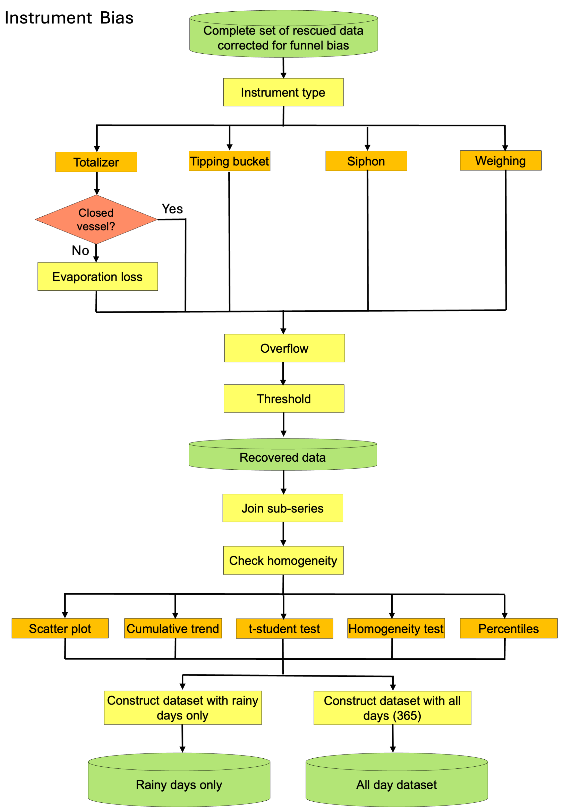
Rain gauges placed in the same site, but at different elevations above the ground, catch different precipitation amounts. This problem was already known in the 18th century [10]. In general, the amount of observed precipitation decreases with the elevation following a parabolic pattern (see Figure 21.15 in [61]). Hutchinson [62] supposed that this difference is due to the condensation of air humidity, which increases the raindrop size as they fall. In the second half of the 19th century, it was understood that the wind field influences the quantity of water collected, but it was not clear to what extent, as the inclination of the drops’ trajectory with respect to the funnel opening depends both on the wind field and the size of the drops: the larger ones fall more undisturbed, while the finer ones tend to follow the horizontal component of the wind. The role of turbulence was also recognized, either generated in proximity to the instrument or to the funnel shape [63].

There is no need to correct modern measurements, because the elevation above the ground of rain gauges is the same for all instruments [7,8], but this is not the case for early ones, as the instruments were located at different heights. Even if the problem is known, the correction is not linear: the comparison of contemporary measurements taken at different elevations in different periods gives different results, where Crestani [11] found that the ratio between the amount collected at the Magrini Observatory, Padua (at 11 m) and at the Astronomical Observatory (24 m) over the 1920–1934 common period was 1.19. If the comparison is extended to the 1920–1980 period, the ratio changes to 1.06 [18].

When measurements collected by different instruments are compared, or data are merged, a correction for the different elevation must be performed. However, care must be taken not to extend a particular correction to other periods and instruments, because each period has its own characteristic that must be analyzed singularly.

Differences of the efficiency of the rain collected is due to the wind field around rain gauges [7]. Different shape of funnels (i.e., square or cylindrical) and exposures (i.e., elevation from the ground and exposure) may introduce discrepancies in the measured precipitation that can be interpreted as climatic signal. It is very difficult to correct this bias, because in most of cases, the wind field in the early period is unknown or measured in a non-standard way. However, this problem is strictly joined with the elevation bias, so the procedures used to this aim can also help to reduce the wind field bias.

3.5. Threshold

The distribution of daily precipitation is strongly skewed, showing high frequencies at low amount and low frequencies at high ones. Candidate functions to represent the daily frequency distribution are hyperbolic function [64], Wakeby distribution, Generalized Extreme Value function [65], gamma, lognormal and normal probability distributions, and Weibull distribution where the skewness is adapted using shape parameters [66,67,68].

Since the most frequent occurrences are at the lowest amounts, a small change in the threshold of an instrument or a small amount of water left undetected in the gauge may significantly change the frequency but leave the amount almost unchanged, especially at monthly and yearly time spans [28].

A similar effect is due to the contribution of dew, hoar, or fog, which do not fit within the definition of precipitation [7]; however, practically, they supply the funnel with water that is recorded as precipitation. In the 18th and 19th centuries, the definition of precipitation also included fog, dew, and so on [9], and therefore, the shape and slope of the funnel (i.e., flat bottom or deep V shaped funnel) play an important role: in V-shaped funnels (i.e., a reversed pyramid, or a cone), condensation drops grow on the inclined surface. When the drops start to move, they join other drops and form rivulets that reach the collector or the counter. This is not a problem for rain, but dew and fog might be measured as rain. Cylindrical or cubic funnels did not have this bias, because of their vertical wall.

The exposure of the funnel on the roof generated another problem: these instruments were connected to a long pipe that drained the rainwater and discharged it into a reservoir placed indoor. In this case, the rain could leave a film of water, or some drops, adherent to the surface of the long pipe, and this water remained undetected, increasing the bulk threshold and potentially reducing the precipitation frequency.

The introduction of modern rain gauges, equipped with heated funnel to avoid dew and hoar, or to melt snow, could lead to a decrease in the recorded precipitation frequency. As an example, on 11 October 2005, the old rain gauge of Legnaro weather station (near Padua) was changed to a heated funnel model. Comparing the precipitation distribution one year before and one later the change, a 6% decrease of the daily frequency of light rain (less than 0.5 mm) was found.

Some types of instruments (i.e., vertical wall and located on the ground) were not affected by this bias, so their data do not need corrections. The others should be corrected, but the amount of the precise correction is unknown, because the original rain gauges are no longer available. The only possibility is the application of a threshold that excludes the data affected by this bias but allows to compare series made by different rain gauges. The value of this threshold should be chosen carefully, after examining the shape of the funnel and its exposure. Fog and dew might be removed by early data without hesitation only if observers recorded them in their observing logs (see also Section 3.7).

The instrumental threshold [28] and the actual definition of a rainy day [69] constitute two critical factors for early and modern series concerning data analysis. When processing a record, one can consider a “rainy day” only the days in which some precipitation has been collected in the rain gauge (definition A). With definition A, in one year, the number of rainy days is ≤365. In addition, by combining the threshold, definition A can be divided in two subclasses, i.e., $A1$, where no threshold is considered or specified, and $A2$, where a threshold is considered, e.g., 0.1 mm as in WMO [8]. Datasets $A1$ are typical of the early period, while datasets $A2$ are typical of the modern period, regulated by the WMO. Alternatively, one can consider rain the output given by the recording instrument, like any other meteorological parameter, and the output may be 0 or different from 0 (definition B). With definition B, the number of rainy days is always 365, except leap years. Of course, the two subsets $A1$ and $A2$ are $\subset B$.

As an example, consider a recording station with a 1 mm threshold, in a location with 110 rainy days a year, and the maximum daily precipitation reaching 80 mm. If we define “rainy day” only as days in which precipitation has been recorded, we obtain a dataset $A2$ with a population of 110 datapoints (which will change every year), and the percentile distribution ranges from 1 (i.e., the 0th percentile) to 80 mm (i.e., the 100th percentile). On the other hand, we can consider rain a meteorological variable where every day the station records the observed value that may range from 0 to 80 mm, i.e., a dataset B. The percentile distribution ranges from 0 (i.e., the 0th percentile) to 80 mm (i.e., the 100th percentile). Both datasets show the same number of days in which rain has fallen, i.e., 110. The dataset A is a subset of B, and the two subsets have the same 100th percentile. However, all the other percentiles are different, and the threshold of A, i.e., 1 mm, is the $100·(365-A)/B$ percentile of B. If an extreme event is defined in terms of percentiles, e.g., the extreme exceeding the 90th percentile [69,70] in the datasets A and B, the percentile distributions are different, and change the actual thresholds for the extreme events, as well as the number of extremes occurred in the station site. This situation is critical because real extremes can be missed or false extremes can be generated.

A consequence of the different definitions of rainy day is shown in Figure 7 for the series of Padua. The lines refer to the ratio $x\mathrm{th}/100\mathrm{th}$ calculated counting rainy days above the threshold only (i.e., definition $A2$, blue lines), and the whole set of the calendar days (i.e., definition B, red lines). Of course, when $x=100$, the result is 1 for both systems. However, when $x=90$, the ratio $90\mathrm{th}/100\mathrm{th}$ of A is largely dominant above the corresponding B value. This is very relevant because extreme events are defined at the 90th percentile threshold: “An extreme weather event is an event that is rare within its statistical reference distribution at a particular place. Definitions of `rare’ vary, but an extreme weather event would normally be as rare as or rarer than the 10th or 90th percentile” [70]. Therefore, the definition of a rainy day, i.e., $A1$, $A2$, B, may transform an extreme event to normal, or vice versa [69].

It must be considered that in Padua, the number of days with precipitation is approximately 110, and those without precipitation is $365-110=255$. According to the definitions, the yearly frequency of rainy days is 110 with A, and 365 with B, of which 225 have null amount. Therefore, A percentiles are calculated on a subset of data (i.e., 110) in comparison with B with the consequence that the most extreme values (i.e., 100th percentile) are the same for both, but they substantially differ at the lower percentiles when the difference between the two definitions become relevant. In particular, in $A2$ all values are larger than zero and the lowest ones coincide with the instrumental threshold, e.g., 0.1 mm. On the other hand, in B, the $255/365=61.6\mathrm{th}$ percentile will be equal to zero, as well as all lower percentiles. This explains why in Figure 7, the B 50th percentile is null while the A 50th percentile is not.

3.6. Observational Protocol

A change in the observational protocol can influence both precipitation amount and frequency. Usually, observers measured and recorded precipitation one or more times per days, but sometimes, the collecting period was longer than a single day. For example, during the 1812–1864 period, the astronomers in Padua read the rain gauge at the end of the rainy events, even if the precipitation continued for more than a single day [54]. When observations were taken irregularly, frequency series were distorted, the number of light rainfalls decreased (Figure 8a), and the percentile distributions increased their values, as well as the extreme events because a single value could include the precipitation of two or more days (Figure 8b). If the rain gauge prevented the evaporation of the collected water, the different reading time affected daily amount, especially in terms of intensity or apparent daily total, not monthly and yearly totals.

Weather notes written by the observer himself were used to correct cumulative amounts, using the proxy technique described in Section 3.1. Notes and comments were compared with the recorded measurements to classify them in three classes: regular (i.e., measurements taken in standard way), cumulative (i.e., measurements taken after some rainy days), and missing (i.e., any data reported in the logs). The amount of the first class has been used to calibrate the proxy series. The quantity estimated by the proxy was used to split the cumulative precipitation amount in the proper days (class cumulative) and to estimate precipitation in the third class [54]. After data correction, the percentile distribution became like the previous and next periods (Figure 8d), even if light rainfalls were not fully recovered (Figure 8c).

3.7. Dew

Following WMO prescriptions, atmospheric condensation (e.g., dew, fog) or formation of ice crystals (e.g., frost, hoar frost, rime) should not be considered as precipitation [8]. However, it is difficult to distinguish light rain from condensation both in automatic, and in manual rain gauges. As already mentioned, in the early period, the observers recorded any amount of water they found into the funnel, without excluding condensation. This bias influenced the precipitation frequency, but less the amount, as the quantity was very small. Modern instruments, with a heated funnel, reduce this problem, because they prevent condensation and frost (see Section 3.5). However, on the other hand, light rainfalls can evaporate, with a drizzle bias.

It is possible to correct the frequency of early series, by analyzing the weather notes, if available. In fact, it is possible to exclude water amounts that correspond to the notes “dew”, “fog”, “condensation”, and so on. This method allows rejecting the amounts of some days in the Padua series (e.g., 23 December 1842; 3 and 10 October 1843) [54]. A careful analysis of the metadata is crucial to address this bias.

3.8. Sampling Time

Modern instruments take digital records at high sampling frequency, so the record is practically continuous, and using software, people can decide how to analyze data, the cumulating period, and the averaging time. WMO recommends avoiding any change in the definition of the climatological day, i.e., the start and the end of the observing window [71]. However, in the past, some observatories considered the observations from midnight to the next midnight, others from 9 a.m. LT (Local Time) to the same hour of the next day, and others selected different starting times. This difference may introduce inhomogeneities, especially in the daily totals and in the analysis of the extremes. If an extreme event happened during the change of the climatological day, it can be lost or underestimated. Changing the extremes of the 24 h recording interval that defines the climatological day may increase or decrease the number of extreme events, or their actual values.

In early periods, the daily precipitation was affected by two problems: the interval between successive measurements, which may be regular or irregular, and the different starting time of the climatological day. At times, both problems were present. Most observers recorded data manually at least one time per day, or more, and the water collected was measured at the beginning, mid, or end of the day, introducing inhomogeneities in long-term series. Sometimes, to avoid evaporation loss, the observer waited for the end of the rain to do the reading. The basic idea was to measure the amount really fallen during the event, without considering that it was distributed within one or two sampling days.

The information on the reading time is often missing in early datasets, and may change in the modern period, depending on the observer choice. The organizations that measured precipitation in Italy started to indicate the climatological day only in the 20th century (

Table 1. Main organizations that measured precipitation in 20th century in Italy and the different starting times of the climatological day.

Name	Period	Starting Time (LT)
Italian Hydrographic Service	1917–1998	09
Meteorological Service of the Italian Air Force (AM)	1951–present	01
Regional Environmental Protection Agency (ARPA)	1993–present	00

).

Figure 9a shows the effects of different definitions of the climatological day on daily percentiles. Using hourly data of the Padua station in the Botanical Garden from 1994 to 2022, daily data has been grouped following the different definitions as in Table 1. To change the starting time from 00 h to 01 h does not introduce biases, while the difference between 00 h and 09 h is evident, especially at high percentiles. Daily frequency is also affected. The confusion matrix [72] allows to compare the number of wet and dry days obtained using the two different definitions of climatological day. In particular, the four quadrants in Figure 9b contain the following relative numbers in a clockwise direction from top right: dry days for both definitions, dry days for 00 h definition that are wet days for 09 h definition, dry days for both, wet days for 00 h that are dry days for 09 h. As a result, nearly 20% of days in 28 years are classified in different way with the 09 h definition.

The difference is even bigger, analyzing the extreme event which occurred on 16th September 2009 (Figure 9c). Using 00 h and 01 h definitions (blue and green lines), the entire amount of precipitation is attributed to 16 September, while using the 09 h definition (red line), rain is split between 16 and 17 September, reducing the entity of the event.

Different methods can be used to correct this bias, as reported in

Table 2. Methods to correct daily rain amount related to different definitions of the climatological day.

Leave measurements unchanged
Shift morning observations back to one calendar day [73,74]
Moving average with a window of two days around the target day [75]
Disaggregation of daily precipitation amounts to hourly and then aggregation back at a different definition of the climatological day	using actual hourly observations [73]
	assuming that daily amount is uniformly distributed across the whole day [74,76];
	using reanalysis models to split daily precipitation to hourly [77]

, by shifting or redistributing the daily amount. However, these corrections should be applied carefully, because they can skew the precipitation statistics, increasing the frequency, introducing temporal autocorrelation to the data, and decreasing the average intensity as well as the extremes [73,74,75,76]. The best solution must be found by testing more methods, because the most proper one depends on datasets, station, and choice of the 24 h measuring period that represents the climatological day.

The modern period of the Padua precipitation series comes from three different organizations with their own standards: Water Magistrate (since 1920 to 1996, 09 h–09 h), Meteorological Service of the Italian Air Force (1951–1990, 01 h–01 h), University of Padua and then ARPA Veneto (since 1980, 00 h–00 h). These data were corrected using the disaggregation method via reanalysis [77], that improved the temporal alignment but increased the precipitation frequency. In general, for the Padua series, all the adjustment methods changed the statistics mainly in summer, the season most affected by heavy rainfalls, and underestimated the percentile values, especially the extremes [77]. Nevertheless, by applying this correction, it would be possible to homogenize precipitation datasets of several Italian stations.

3.9. Full Vessel

As in the early period the water collected in rain gauges was not measured regularly, even if vessels were large, it may happen that the water filled the collecting vessel, a problem that was exacerbated by the combination of long-time interval between measurements and heavy rainfalls. The precipitation amount is affected, but not the frequency. This is crucial in the analysis of extreme events, because the amount of heavy rain is underestimated.

This bias is not common, but difficult to detect, except when there is a recurrent value for the maximum collected amount, i.e., the vessel capacity. In the metadata, observers never wrote the vessel capacity, but sometimes, in the logs, a comment on this overflow problem was reported.

As it is not possible to estimate the precipitation that has fallen after the filled vessel, it is better to keep the original value, even if it is an underestimation. If the observes commented “rain gauge full” or similar expressions, it is possible to estimate the maximum amount of the vessel and recognize other similar cases even if the observer did not write any comment.

4. Compatibility Between Subseries

To compose a long continuous precipitation series, it is necessary to merge the different subseries that have been reconstructed and corrected individually. To do this, some statistical and mathematical approach can be used, depending on whether the series have overlapping periods or not. These statistical tests can be applied to any series, whether early or modern, as they are specifically intended to investigate the presence of potential discontinuities. The research and understanding of metadata are crucial to interpret any discontinuities and determine whether they should be attributed to climate change or to other factors. While this process is relatively straightforward for modern series, it is much more complex for early series due to the difficulty in finding and interpreting the metadata.

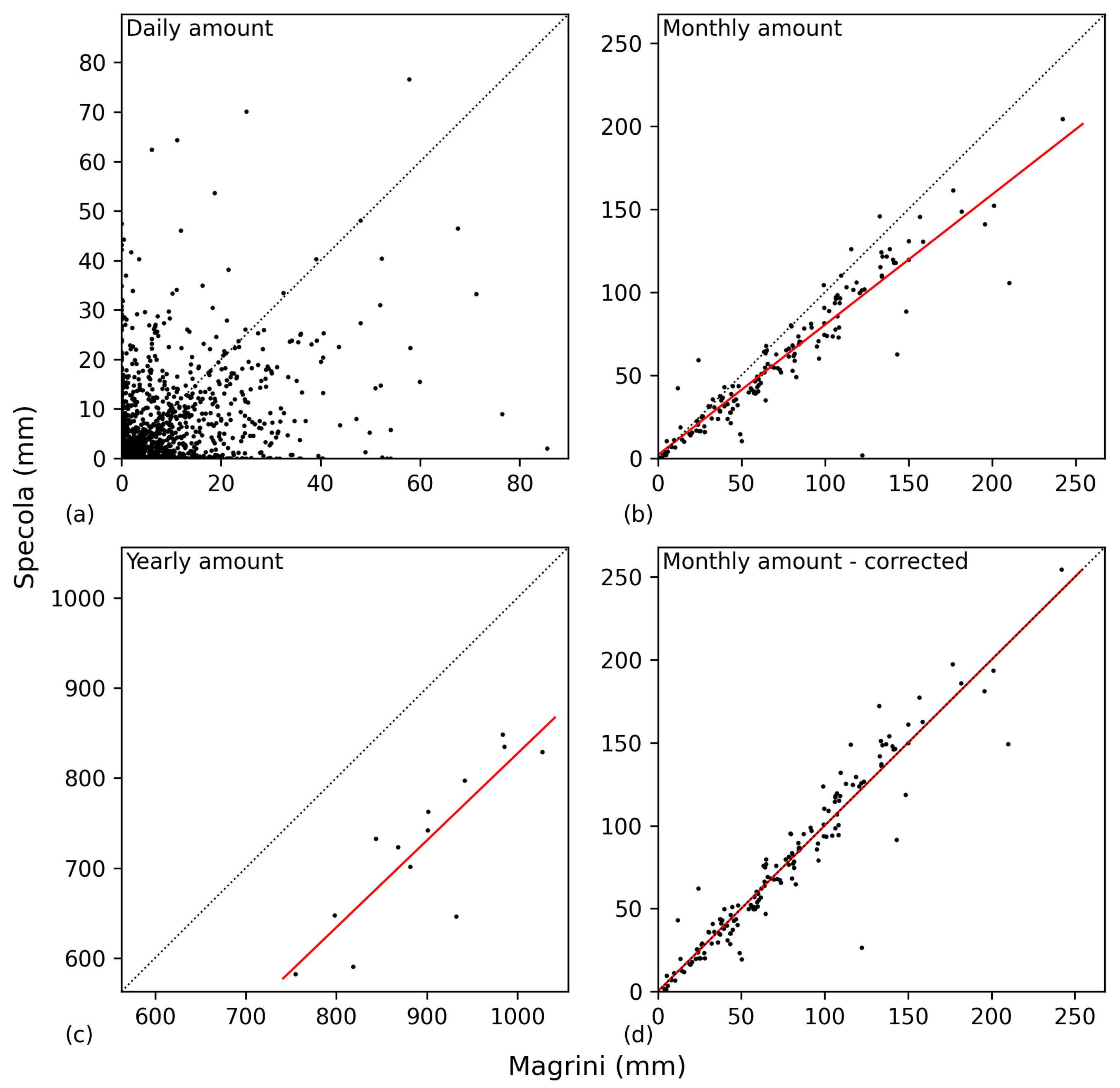
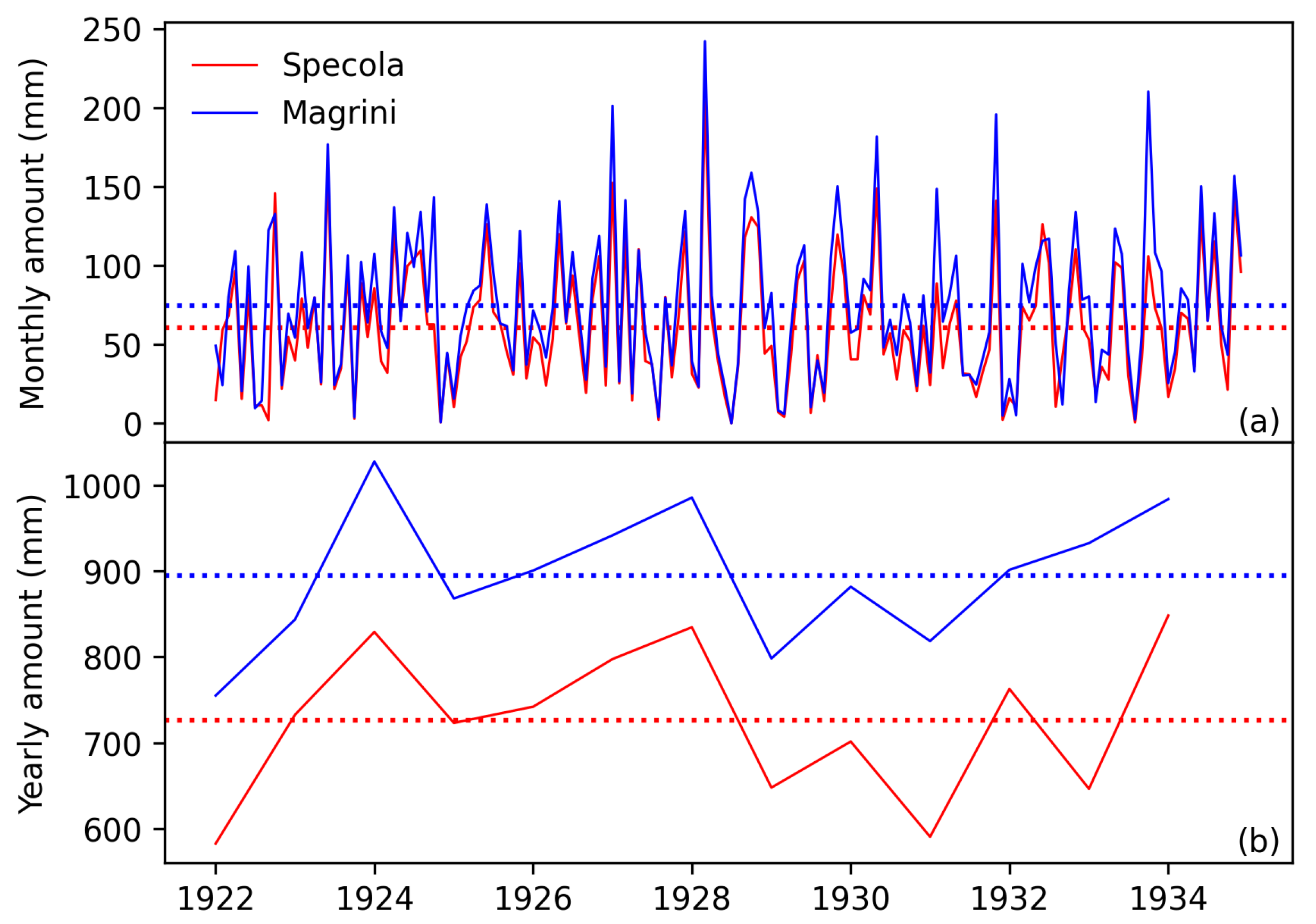
4.1. Direct Comparison of Overlapping Periods

The simplest test is to overlap common (sub)periods of two contemporary series, if any. This method can be applied to daily, monthly, and yearly precipitation amounts. In the following examples, the data of two subseries of Padua are used: the 1922–1934 subseries of the Astronomical Observatory (in the following “Specola”) and the 1922–1979 subseries of the Meteorological Observatory “Magrini” of the Water Magistrate. It is well known [19] that the last period of the “Specola” has different problems, and it was not used to compose the long series of Padua. Therefore, its data is useful to illustrate the following method.

The comparison of daily amounts (Figure 10a) is difficult, because the values are too scattered. This high variability is a combination of various factors as the different sampling time (see Section 3.8). The linear interpolation has very low $R^2=0.12$.

The comparison of monthly amounts gives a better result. The points are well aligned, and only a few of them scatter from the mean. This is due mainly for the different sampling time of the day between two subsequent months, and local events that happened over only one of the stations. The interpolation line has a good $R^2=0.87$ and shows that the precipitation measured by “Specola” is underestimated, so correction is needed, before joining the two subseries. The correction can be made considering that a strict alignment of data implies that the interpolation line is coincident with the bisector (i.e., the line with the equation $y=x$).

A generic line is defined by the equation $y=mx+q$, where m is the slope and q is the intercept. The equation of the interpolation line of the original, raw data is

$$y_r=m_{r}x+q_r$$

(1)

where the subscript r is the original uncorrected data, and

$$y_c=m_{c}x+q_c$$

(2)

is the equation of the interpolation line of corrected data, with subscript c. The correction that should be applied to the raw data is

$$\Delta y=y_r-y_c=(m_r-m_c)x+q_r-q_c$$

(3)

Since $y_c=y_r-\Delta y$, and in this case $m_c=1$, $q_c=0$ (equation of bisector line), Equation (2) becomes

$$y_c=y_r-(m_r-1)x+q_r$$

(4)

The result of the correction of monthly data is shown in Figure 10d. Note that the interpolation line of corrected data perfectly overlaps the bisector line, and the $R^2$ is higher than the original one ($R^2=0.92$).

Finally, the differences of the yearly amounts are smoothed, but the number of points is lower (only 13). The interpolation is good, with $R^2=0.73$, and confirms the underestimation of the Specola amount over the 1922–1934 period. In this case, the correction is feasible, despite the low number of data, and Equation (4) can be applied.

The scatter plot method can be used to correct monthly series and yearly series (depending on the number of overlapping years), though rarely daily series.

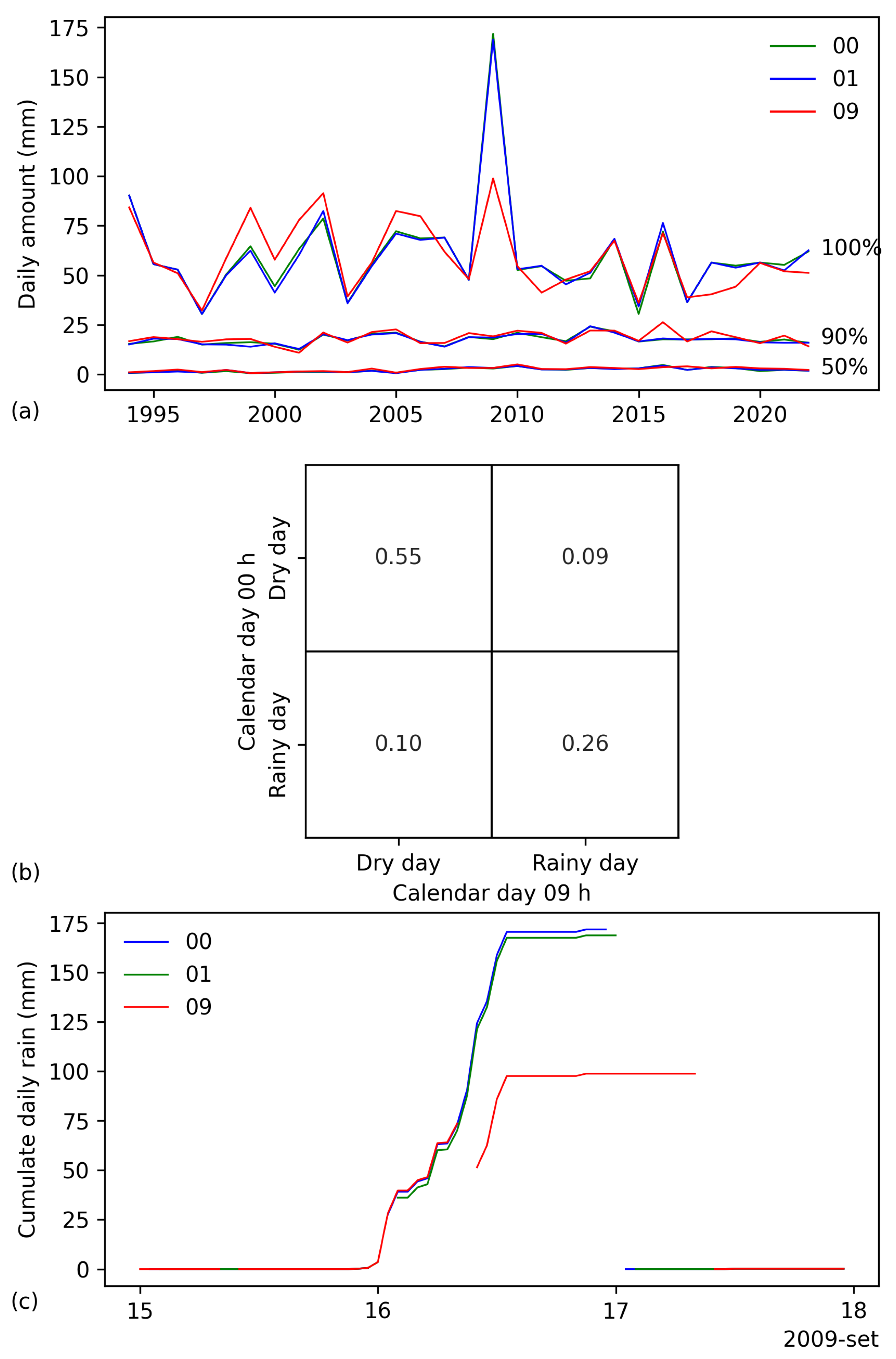
4.2. Cumulate Method

Another useful method to compare subseries is the comparison of the cumulate trends. The cumulate amount can be calculated starting from daily or monthly amounts. The cumulate highlights the average trend of the precipitation series and allow to identify changes. Figure 11 shows the application of this method to the same Padua stations used in Section 4.1. The two cumulate curves have a linear trend, and the interpolation lines show in a different manner the underestimation of the precipitation measured by “Specola” from 1922 to 1934. The cumulate methodology is more efficient than the scatter plot to compare data, especially when the overlapping period is not long enough. Since the intercept of the two interpolation lines is zero, Equation (3) becomes

$$y_c=y_r-(m_r-m_c)x$$

(5)

which can be used to correct raw data at daily, monthly, or yearly resolution. The cumulate method does not require the subseries to overlap; they can also be adjacent.

4.3. Student’s t-Test

If the two subseries have gaps that cannot be resolved (see Section 3.1) or their records have different time resolution, the two-sample Student’s t-test [67,78] can be used to verify if the mean values of the two subseries are compatible. The null hypothesis of Student’s t-test states that the difference between the two datasets is zero, the alternative hypothesis that is not zero, or that one of the two underlying means is larger than the other. For overlapping datasets, the hope is that the test validates the null hypothesis. Unfortunately, Student’s t-test requires the condition that the two datasets have a Gaussian distribution [67]. It is well known that this is not true for daily precipitation amount, but the distributions of the monthly and yearly amounts can be considered Gaussian as a first approximation.

Student’s t-test applied to the monthly and yearly datasets of “Magrini” and “Specola” subseries confirms the alternative hypothesis, i.e., that they are not compatible and cannot be joined without correction (see Figure 12).

In Figure 12, the “Magrini” and “Specola” subseries are compared both at monthly and yearly resolutions. In the monthly time plot (Figure 12a), the differences between the two datasets are not so clear, so it is better to use the scatter (Figure 12b) or the cumulate plots (Figure 11) for a direct comparison of the overlapping periods of two subseries.

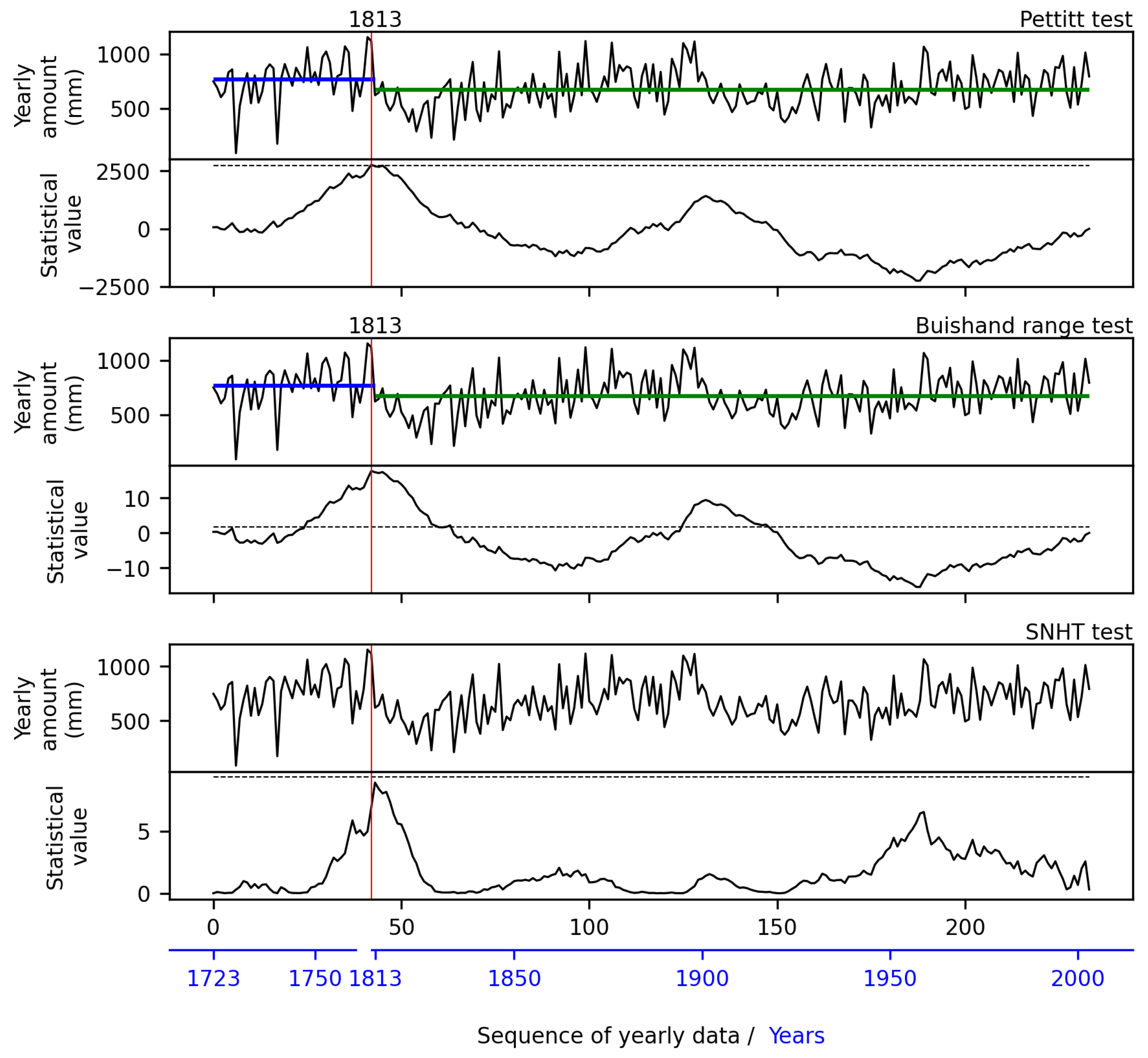
4.4. Homogeneity Tests

If there are no overlapping periods, and two or more subseries are separated by gaps, several homogeneity tests can be used to detect discontinuities, and regime shifts in precipitation series. Homogeneity tests can be relative or absolute. The first are generally favored over absolute ones as they use the difference between the time series of the target station and the ones of the neighboring stations to identify breaks or change points [79]. Moreover, they can detect multiple change points in the same analysis. However, relative tests are hardly applicable to early instrumental series because records from neighboring stations are generally not available or because observing protocols are not compatible with each other. Moreover, the reference records should have the same climate as the target station, and this is not always true, as discussed in Section 2.2.

The most-used absolute tests to identify change points are: Standard Normal Homogeneity Test (SNHT) [80], Buishand U test (BU) [81], Pettitt test [82], and von Neumann ratio (VN) [83]. All these tests, except VN, give information on the timing of the change point. The BU and Pettitt tests usually perform better when a break appears in the middle of the series, whereas SNHT is better in identifying inhomogeneities at the beginning/end. For this reason, these tests are often used simultaneously.

The null hypothesis of these tests is that the values of the dataset are independent and identically distributed; the alternative hypothesis is that a change point in the mean is present. To find out which of the two hypotheses occurs, each test calculates a statistical value from the amount of precipitation. If this value is above a critical parameter (threshold), the null hypothesis is rejected. The mathematical formulation of these four tests and their critical parameters can be found in the original works [80,81,82,83] and in Appendix A of Wijngaard et al. [84]. In the literature, these tests are usually applied to monthly, seasonally, or yearly precipitation series [84,85,86,87]). When all these tests are used, the dataset can be classified as [84]:

• Useful: one or zero tests reject the null hypothesis;
• Doubtful: two tests reject the null hypothesis;
• Suspect: three or four tests reject the null hypothesis.

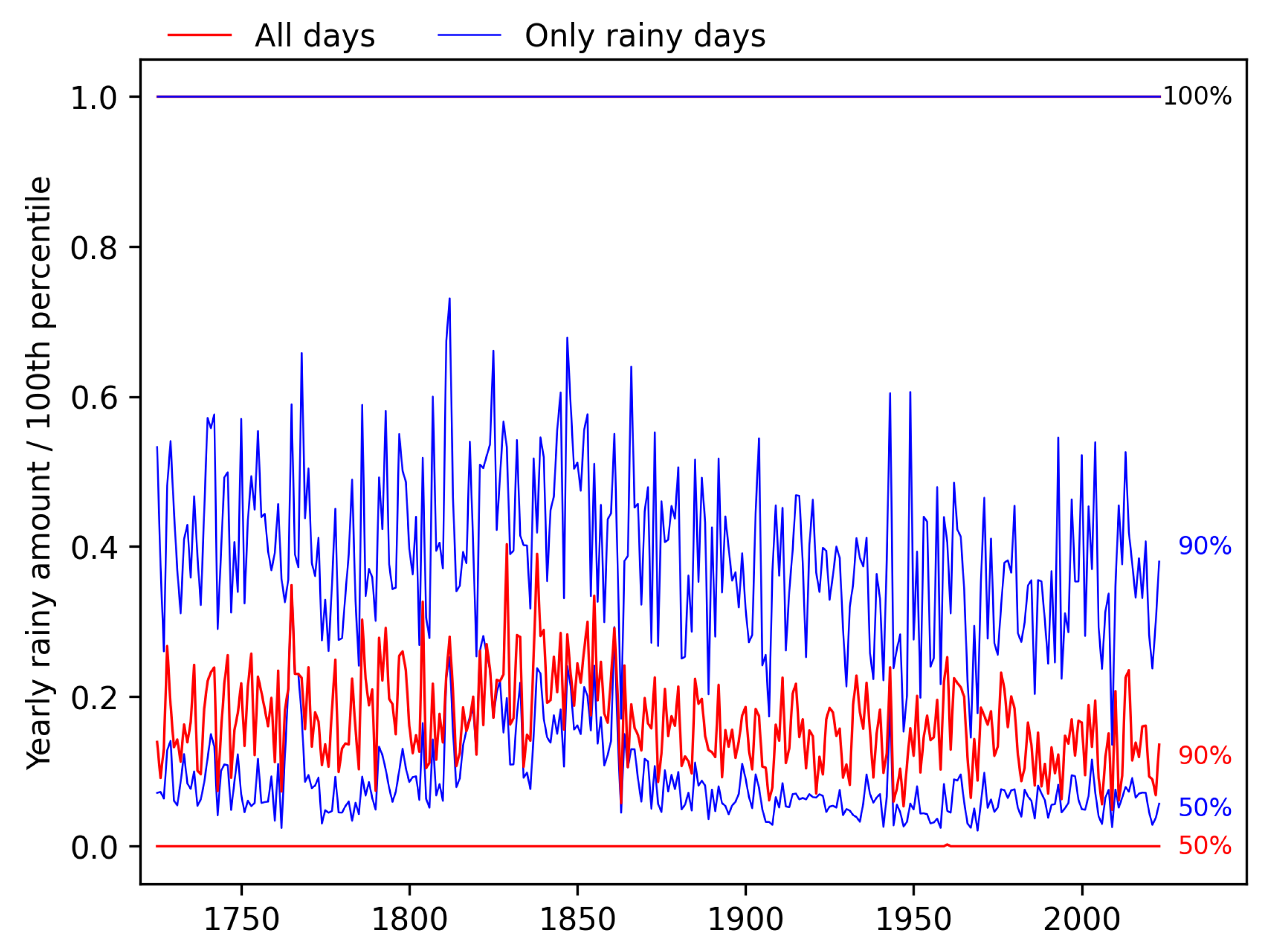
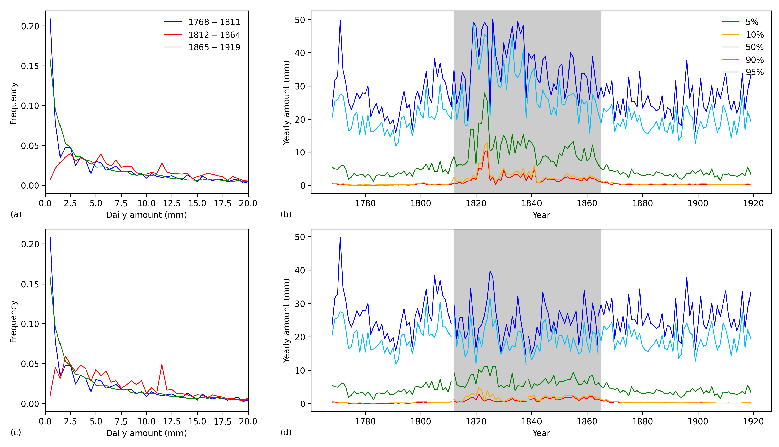
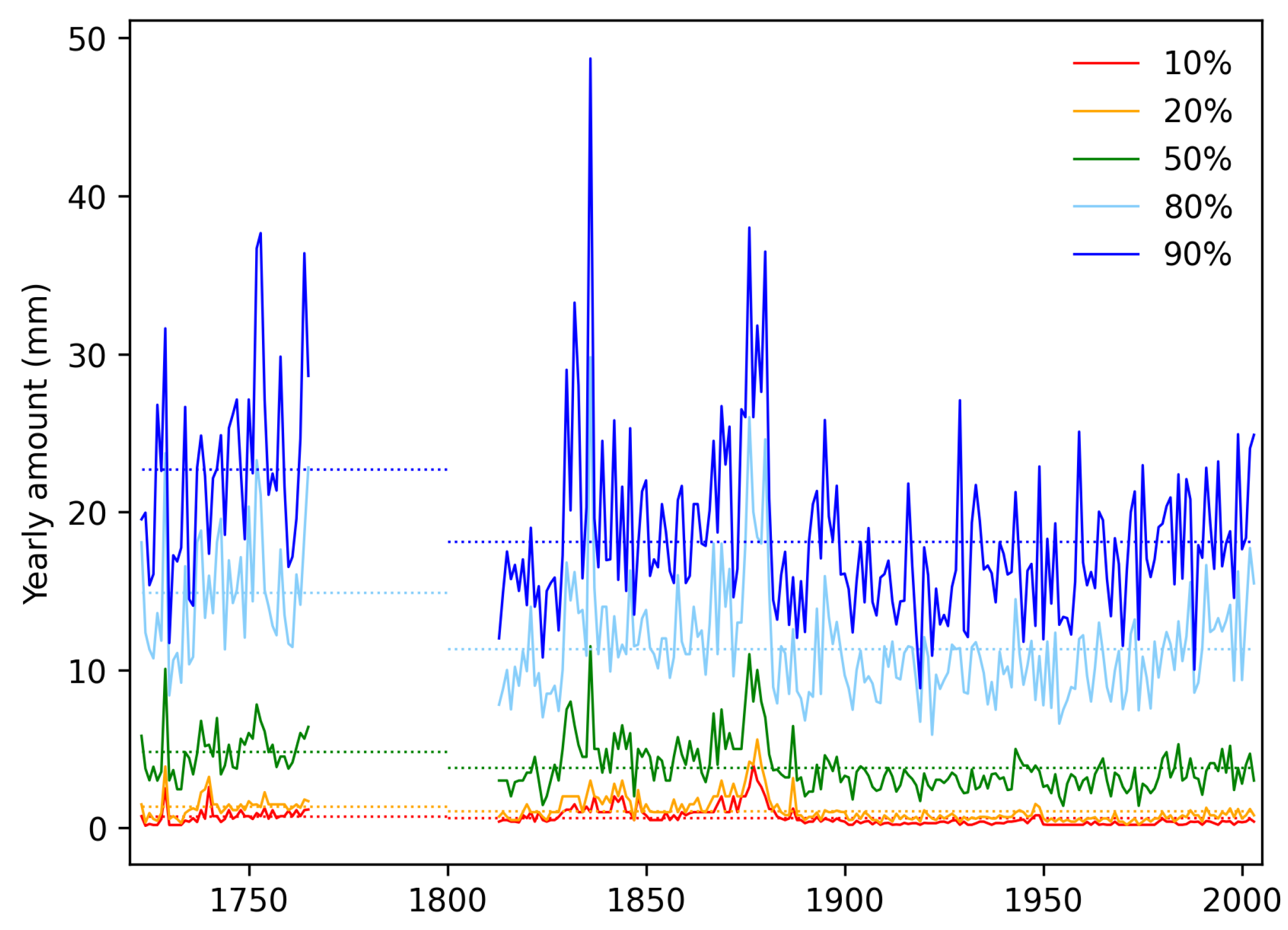
The homogeneity tests have been applied to the yearly amounts of the Bologna series, composed of two main subseries: the 1723–1765 period, where the measurements were made by Jacopo Bartolomeo Beccari, and the 1813–2003 period, where measurements were made by the astronomers of the Astronomical Observatory and then by the Ufficio Idrografico (Hydrographic Office). Since the homogeneity tests require a continuous dataset, before the calculation, the 48-year gap has been eliminated, and the end of the first period has been put to coincide with the beginning of the second one. In this manner, a continuous sequence of data has been created: the main scale in the abscissa of Figure 13 (black color) refers to the position in the continuous sequence of values. A second scale (blue color) has been added to show the right temporal sequence. A vertical red line highlights the position where the gap collapsed.

Both Pettitt and BU homogeneity tests reveal a change point in the year 1813. Also, the VN test confirms that these data are not homogeneous. Since three of the four tests have rejected the null hypothesis in the same year, the dataset cannot be considered homogeneous [84], and further investigation and analysis is needed before merging the two subseries, to understand the nature of the discontinuity. In this specific case, this is not a climatic signal, but rather attributable to a change in measurement location and observer, and therefore, it must be corrected. The dashed lines in Figure 13 highlight the 5% critical values. Blue and green lines are the mean values before and after the change point. These values have been used to homogenize the two subseries, removing the differences between them.

4.5. Percentiles

Percentiles distributions can be used to check the homogeneity without complex statistical tools, because they are influenced by the characteristic of the instrument used: low percentiles depend on the instrument threshold (Section 3.5) and high percentiles depend on the amount of water collected in the vessel (wind field and elevation, see Section 3.4). Also, the use of different observing protocols alters the whole percentile distribution (Section 3.6).

When a daily precipitation series is available, the yearly percentile distribution can be calculated to highlight if there are differences between two subseries. As explained in Section 3.5, percentile distributions can be calculated in two ways: considering only rainy days or the whole number of calendar days (i.e., 365 days). The first way is better to check differences between two subseries, because it is more sensitive to the low percentile values (see Figure 7).

In Figure 14, some percentiles of the subseries of Bologna are shown. The smallest percentiles (10th and 20th) show low differences between the two subperiods, which suggests that the instruments had different thresholds. The 50th (median), 80th, and 90th percentiles have different trends, and this can be explained with instruments at different elevations (home of Beccari and tower of Astronomical Observatory). Again, the cross comparison between the results of the statistical tests and the information collected in the metadata allows to understand the origins of the discontinuities in a precipitation series.

5. Conclusions

This paper describes the main issues to be faced when recovering and reconstructing early precipitation series and provides a methodology to address and resolve them. The methodology is structured in three stages, each of which is composed of several steps that cannot be skipped. The retrieval and critical analysis of metadata is crucial but difficult for the early period, as it is essential for accurately reconstructing the series and distinguishing biases from the climatic signal.

Once data have been rescued and copied, some problems must be analyzed and solved: the conversion from original to modern units; different observational protocols; shape, location, and exposure of funnels and rain gauges; and time and frequency of observations. All these aspects need to be examined carefully, using not only the measured values reported, but all the information written by the observers, especially weather comments. However, sometimes, metadata are scarce or missing, and the information concerning instruments must be extracted from the data itself, or using other sources (e.g., correspondence between scientists, reports, or publications), if any.

A multidisciplinary approach which includes a thorough analysis of original sources is needed, and this can be extremely difficult as the sources are often in old languages, with unusual terms and hardly readable, as they are hand-written.

Another difficulty consists of gaps, or other problems caused by the impossibility of making comparisons with other contemporary series in neighboring locations, and the different methodologies used to measure precipitation. In these cases, proxy data can be used to complete gaps or missing periods. It should be noted that it is impossible to correct any specific form of bias individually (e.g., instrument, observing protocol, exposure, wind drag), while it may be possible to apply a bulk correction that includes all the existing biases. Therefore, monthly or yearly amounts may be corrected, not individual events. This is not a problem for average values but becomes a serious problem in the long-term analysis of the extreme events, their distribution, and trends.

The definition of a ‘rainy day’ is a problem that also affects modern series, as it concerns data analysis, and must be applied to a precipitation dataset, regardless of how it was obtained. This issue is influential to the analysis of extreme events. In fact, one can consider three options, i.e., every day in which precipitation has been recorded, only days in which the precipitation amount exceeds a certain instrumental threshold, or every day of the calendar year, with an amount equal to or different from 0. The choice may significantly affect the 90th percentile, which is the threshold recommended by the IPCC 2014 to define whether an event is extreme or not.

Finally, when an early precipitation record is combined with a modern one, the problem of homogeneity must be solved, because early data were taken with different methods and instruments. Therefore, if this fact is accepted as an unavoidable consequence of using old dataset, it is possible to distinguish changes due to other historical reasons than climate change.

This is the first time that a methodology for handling early precipitation series is presented in a comprehensive manner, describing each potential issue that may arise and how to resolve it, when a solution is possible. The recovery and reconstruction of long meteorological series is extremely important for the calibration of climate models, and uncorrected datasets may introduce inhomogeneities that risk to hide or misinterpret the extent of climate changes.

In conclusion, this paper puts in evidence that mathematical and statistical methods are very important in the complex work of reconstructing and correcting an early meteorological series, but at the same time, they are not exhaustive. Moreover, they cannot be applied to raw data, as the data itself must first be carefully analyzed together with the metadata to identify and correct problems and biases, and finally, to obtain a series on which climate studies can be carried out.

Furthermore, it is good to clarify what is meant by a multidisciplinary approach. As this paper envisages, it does not simply consist of merely speculative historical research, but of reliving the history of the series by putting oneself in the shoes of the operator of the time and its culture. Only in this way can one understand the problems that affected data and develop sound and reliable methods for their correction.

References

1. Marchi, M.; Castellanos-Acuña, D.; Hamann, A.; Wang, T.; Ray, D.; Menzel, A. ClimateEU, scale-free climate normals, historical time series, and future projections for Europe. Sci. Data 2020, 7, 428. [Google Scholar] [CrossRef]
2. Lundstad, E.; Brugnara, Y.; Pappert, D.; Kopp, J.; Samakinwa, E.; Hürzeler, A.; Andersson, A.; Chimani, B.; Cornes, R.; Demarée, G.; et al. The global historical climate database HCLIM. Sci. Data 2023, 10, 44. [Google Scholar] [CrossRef] [PubMed]
3. Flaounas, E.; Davolio, S.; Raveh-Rubin, S.; Pantillon, F.; Miglietta, M.M.; Gaertner, M.A.; Hatzaki, M.; Homar, V.; Khodayar, S.; Korres, G.; et al. Mediterranean cyclones: Current knowledge and open questions on dynamics, prediction, climatology and impacts. Weather Clim. Dyn. 2022, 3, 173–208. [Google Scholar] [CrossRef]
4. Authority of the Meteorological Committee. Protocols and and Appendices. In Report of the Proceedings of the Meteorological Congress at Leipzig in 1783; Her Majesty’s Stationary Office: London, UK, 1873. [Google Scholar]
5. Camuffo, D.; della Valle, A.; Becherini, F. Instrumental and Observational Problems of the Earliest Temperature Records in Italy: A Methodology for Data Recovery and Correction. Climate 2023, 11, 178. [Google Scholar] [CrossRef]
6. Sevruk, B.; Hamon, W. Operational Hydrology. Report No. 21. Methods of Correction for Systematic Error in Point Precipitation Measurement for Operational Use; Vol. WMO No 589; World Meteorological Organization: Geneva, Switzerland, 1982; Available online: https://library.wmo.int/idurl/4/33639 (accessed on 15 April 2025).
7. World Meteorological Organization. Instruments and Observing Methods Report No. 39; Vol. WMO/TD-No. 313; World Meteorological Organization: Geneva, Switzerland, 1989; Available online: https://library.wmo.int/idurl/4/41708 (accessed on 15 April 2025).
8. World Meteorological Organization. Guide to Instruments and Methods of Observation; Vol. WMO-No. 8, I; World Meteorological Organization: Geneva, Switzerland, 2023; Available online: https://library.wmo.int/idurl/4/68695 (accessed on 15 April 2025).
9. Toaldo, G. Della Vera Influenza degli Astri, delle Stagioni e delle Mutazioni di Tempo, Saggio Meteorologico; Manfré: Padua, Italy, 1770. [Google Scholar]
10. Heberden, W. Of the quantities of rain which appear to fall at different heights over the same spot of ground. Philos. Trans. 1769, 59, 359–362. [Google Scholar]
11. Crestani, G. Studio Storico Critico. In Le Precipitazioni Atmosferiche a Padova; Ministero dei Lavori Pubblici, Ufficio Idrografico: Rome, Italy, 1935. [Google Scholar]
12. World Meteorological Organization. Manual on the WMO Integrated Global Observing System. Annex VIII to the WMO Technical Regulations; Vol. WMO-No. 1160; World Meteorological Organization: Geneva, Switzerland, 2024; Available online: https://library.wmo.int/idurl/4/55063 (accessed on 6 June 2025).
13. World Meteorological Organization. Guide to the Global Observing System; Vol. WMO-No. 488; World Meteorological Organization: Geneva, Switzerland, 2017; Available online: https://library.wmo.int/idurl/4/35699 (accessed on 6 June 2025).
14. Cantù, V. The Climate of Italy. In World Survey of Climatology—Climates of Central and Southern Europe; Landsberg, H., Ed.; Elsevier: Amsterdam, The Netherlands, 1977; Volume 7, pp. 127–183. [Google Scholar]
15. Tilli, G.L. Acqua di Pioggia passata per la Pevera del Giardino dei Semplici in quest’Anno 1775. Mag. Toscano 1776, 26, 138–139. [Google Scholar]
16. Vallisneri, A. Lezione Accademica Intorno all’Origine delle Fontane, 2nd ed.; Pietro Poletti: Venice, Italy, 1726; pp. 1–365. [Google Scholar]
17. Rapetti, F.; Ruschi, M. Osservazioni botanico-meteorologiche condotte da Giovanni Lorenzo Tilli presso il Giardino dei Semplici di Pisa (1775–1780). Atti Soc. Toscana Sci. Nat. Mem. 2009, 114, 45–59. Available online: http://www.stsn.it/images/pdf/serA114/Rapetti%20Ruschi%202009.pdf (accessed on 15 April 2025).
18. Camuffo, D. Analysis of the series of precipitation at Padova, Italy. Clim. Change 1984, 6, 57–77. [Google Scholar] [CrossRef]
19. Camuffo, D.; Becherini, F.; della Valle, A.; Zanini, V. Three centuries of daily precipitation in Padua, Italy, 1713–2018: History, relocations, gaps, homogeneity and raw data. Clim. Change 2020, 162, 923–942. [Google Scholar] [CrossRef]
20. Camuffo, D.; Becherini, F.; della Valle, A. The Beccari series of precipitation in Bologna, Italy, from 1723 to 1765. Clim. Change 2019, 155, 359–376. [Google Scholar] [CrossRef]
21. Camuffo, D.; Becherini, F.; della Valle, A.; Zanini, V. A comparison between different methods to fill gaps in early precipitation series. Environ. Earth Sci. 2022, 81, 345. [Google Scholar] [CrossRef]
22. Jurin, J. Invitatio ad observationes Meteorologicas communi consilio instituendas a Jacobo Jurin M. D. Soc. Reg Secr et Colleg Med Lond Socio. Philos. Trans. 1723, 379, 422–427. [Google Scholar]
23. Hemmer, J. Descriptio instrumentorum meteorologicorum, tam eorum, quam Societas distribuit, quam quibus praeter haec Manheimii utitur. Ephemer. Soc. Meteorol. Palatinae 1783, 1, 57–90. [Google Scholar]
24. Cotte, L. Mémoires sur la Météorologie pour Servir de Suite et de Supplément au Traité de Météorologie Publié en 1774; Imprimerie Royale: Paris, France, 1774. [Google Scholar]
25. Leutmann, J. Instrumenta Meteorognosiae Inservientia; Zimmermann: Wittemberg, Germany, 1725. [Google Scholar]
26. Poleni, G. Johannis Poleni Miscellanea hoc est: I Dissertatio de Barometris et Termometris; Aloysium Pavinum: Venice, Italy, 1709. [Google Scholar]
27. Burnings, C. Bericht wegens een’ nieuwen hyethometer. In Vederhandelingen uitgegeeven door de Hollandsche Maatschappye der Weetenschappen; Walré: Haarlem, The Netherlands, 1789; pp. 317–323. [Google Scholar]
28. Camuffo, D.; Becherini, F.; della Valle, A. How the rain-gauge threshold affects the precipitation frequency and amount. Clim. Change 2022, 170, 7. [Google Scholar] [CrossRef]
29. Buchardat, A. Fisica Elementare; Filiatre Sebezio: Naples, Italy, 1814. [Google Scholar]
30. Marvin, C. Measurement of Precipitation; US Department of Agricolture, Weather Bureau. Government Printing Office: Washington, DC, USA, 1913. [Google Scholar]
31. Eredia, F. Gli Strumenti di Meteorologia ed Aerologia; Bardi: Rome, Italy, 1936. [Google Scholar]
32. Caldera, H.P.G.M.; Piyathisse, V.R.P.C.; Nandalal, K.D.W. A Comparison of Methods of Estimating Missing Daily Rainfall Data. Eng. J. Inst. Eng. Sri Lanka 2016, 49, 1–8. [Google Scholar] [CrossRef]
33. Longman, R.J.; Newman, A.J.; Giambelluca, T.W.; Lucas, M. Characterizing the Uncertainty and Assessing the Value of Gap-Filled Daily Rainfall Data in Hawaii. J. Appl. Meteorol. Climatol. 2020, 59, 1261–1276. [Google Scholar] [CrossRef]
34. Aieb, A.; Madani, K.; Scarpa, M.; Bonaccorso, B.; Lefsih, K. A new approach for processing climate missing databases applied to daily rainfall data in Soummam watershed, Algeria. Heliyon 2019, 5, e01247. [Google Scholar] [CrossRef]
35. Bellido-Jiménez, J.A.; Gualda, J.E.; Garcìa-Marìn, A.P. Assessing Machine Learning Models for Gap Filling Daily Rainfall Series in a Semiarid Region of Spain. Atmosphere 2021, 12, 1158. [Google Scholar] [CrossRef]
36. Pfister, L.; Brönnimann, S.; Schwander, M.; Isotta, F.A.; Horton, P.; Rohr, C. Statistical reconstruction of daily precipitation and temperature fields in Switzerland back to 1864. Clim. Past 2020, 16, 663–678. [Google Scholar] [CrossRef]
37. Crestani, G. L’inizio delle osservazioni meteorologiche a Padova. Il contributo di Giovanni Poleni alla meteorologia. In Memorie della R. Accademia di Scienze Lettere ed Arti; Rondi, G. B.: Padua, Italy, 1926; Volume XLII, pp. 19–83. [Google Scholar]
38. Crestani, G. Le osservazioni meteorologiche—I fenomeni meteorologici. In La laguna di Venezia; Magrini, G., Ed.; Ferrari: Venice, Italy, 1933; Volume I, Part II, Tomo III, pp. 1–203. [Google Scholar]
39. Rodrigo, F.S.; Esteban-Parra, M.J.; Castro-Diez, Y. An attempt to reconstruct the rainfall regime of andalusia (southern Spain) from 1601 A.D. to 1650 A.D. using historical documents. Clim. Change 1994, 27, 397–418. [Google Scholar] [CrossRef]
40. Dominguez-Castro, F.; Garcìa-Herrera, R.; Vaquero, J.M. An early weather diary from Iberia (Lisbon, 1631–1632). Weather 2015, 70, 20–24. [Google Scholar] [CrossRef]
41. Fernández-Fernández, M.I.; Gallego, M.C.; Domínguez-Castro, F.; Trigo, R.M.; Vaquero, J.M. The climate in Zafra from 1750 to 1840: Precipitation. Clim. Change 2015, 129, 267–280. [Google Scholar] [CrossRef]
42. Santos, J.A.; Carneiro, M.F.; Alcoforado, M.J.; Leal, S.; Luz, A.L.; Camuffo, D.; Zorita, E. Calibration and multi-source consistency analysis of reconstructed precipitation series in Portugal since the early 17th century. Holocene 2015, 25, 663–676. [Google Scholar] [CrossRef]
43. Alcoforado, M.J.; de Fátima Nunes, M.; Garcia, J.C.; Taborda, J.P. Temperature and precipitation reconstruction in southern Portugal during the late Maunder Minimum (AD 1675–1715). Holocene 2000, 10, 333–340. [Google Scholar] [CrossRef]
44. Gimmi, U.; Luterbacher, J.; Pfister, C.; Wanner, H. A method to reconstruct long precipitation series using systematic descriptive observations in weather diaries: The example of the precipitation series for Bern, Switzerland (1760–2003). Theor. Appl. Climatol. 2007, 87, 185–199. [Google Scholar] [CrossRef]
45. Ge, Q.S.; Zheng, J.Y.; Hao, Z.X.; Zhang, P.Y.; Wang, W.C. Reconstruction of historical climate in China: High-Resolution Precipitation Data from Qing Dynasty Archives. Bull. Am. Meteorol. Soc. 2005, 86, 671–680. [Google Scholar] [CrossRef]
46. Brázdil, R.; Chromá, K.; Valášek, H.; Dolák, L. Hydrometeorological extremes derived from taxation records for south-eastern Moravia, Czech Republic, 1751–1900 AD. Clim. Past 2012, 8, 467–481. [Google Scholar] [CrossRef]
47. Harvey-Fishenden, A.; Macdonald, N. Evaluating the utility of qualitative personal diaries in precipitation reconstruction in the eighteenth and nineteenth centuries. Clim. Past 2021, 17, 133–149. [Google Scholar] [CrossRef]
48. Diodato, N. Climatic fluctuations in southern Italy since the 17th century: Reconstruction with precipitation records at Benevento. Clim. Change 2007, 80, 411–431. [Google Scholar] [CrossRef]
49. Raicich, F. Some features of Trieste climate from an eighteenth century diary (1732–1749). Clim. Change 2008, 86, 211–226. [Google Scholar] [CrossRef]
50. Derham, W. Tables of the barometrical altitudes at Zuerich in Switzerland in the year 1708, observed by John James Scheuchzer, F.R.S. and at Upminster in England, observed at the same time by Mr W. Derham, F.R.S., and also the Rain at Pisa in Italy in 1707 and 1708 observed there by Dr Michael Angelo Tilli, F.R.S., and at Zurich in 1708 and at Upminster in all that time. Philos. Trans. 1710, 26, 342–366. [Google Scholar]
51. Derham, W. Physico-Theology: Or, a Demonstration of the Being and Attributes of God, from His Works of Creation; Innys: London, UK, 1713. [Google Scholar]
52. Winkler, P. The early meteorological network of the Societas Meteorologica Palatina (1781–1792): Foundation, organization, and reception. Hist. Geo- Space Sci. 2023, 14, 93–120. [Google Scholar] [CrossRef]
53. Pietropoli, G. Relazione meteorologica dell’anno 1838. In Giornale Astro-Meteorologico per l’anno 1840; Tipografia del Seminario: Padua, Italy, 1839; pp. 41–54. [Google Scholar]
54. della Valle, A.; Camuffo, D.; Becherini, F.; Zanini, V. Recovering, correcting, and reconstructing precipitation data affected by gaps and irregular readings: The Padua series from 1812 to 1864. Clim. Change 2023, 176, 9. [Google Scholar] [CrossRef]
55. Goodison, B.; Ferguson, H.; McKay, G. Comparison of point snowfall measurement techniques. In Handbook of Snow; Gray, D., Male, M., Eds.; Pergamon: Tarrytown, NY, USA, 1981; pp. 200–210. [Google Scholar]
56. Sevruk, B.; Hamon, W. Instrument and Observing Methods. Report No. 17. International Comparison of National Precipitation Gauges with a Reference pit Gauge; Vol. WMO/TD No. 38; World Meteorological Organization: Geneva, Switzerland, 1984; Available online: https://library.wmo.int/idurl/4/41740 (accessed on 15 April 2025).
57. Lanza, L.; Leroy, M.; Alexadropoulos, C.; Stagi, L.; Wauben, W. Instruments and Observing Methods. Report No. 84. The WMO Laboratory Intercomparison of Rainfall Intensity Gauges: Final Report; Vol. WMO/TD No. 1304; World Meteorological Organization: Geneva, Switzerland, 2006; Available online: https://library.wmo.int/idurl/4/35348 (accessed on 15 April 2025).
58. Mariotte, M. Traité du Mouvement des Eaux et des Autres Corps Fluides; Chez Estienne Michallet: Paris, France, 1686. [Google Scholar]
59. Sevruk, B. Evaporation losses from containers of Hellmann precipitation gauges. Hydrol. Sci. Bull. 1974, 19, 231–236. [Google Scholar] [CrossRef]
60. Leeper, R.D.; Kochendorfer, J. Evaporation from weighing precipitation gauges: Impacts on automated gauge measurements and quality assurance methods. Atmos. Meas. Tech. 2015, 8, 2291–2300. [Google Scholar] [CrossRef]
61. Camuffo, D. Microclimate for Cultural Heritage, 3rd ed.; Elsevier: Amsterdam, The Netherlands, 2019. [Google Scholar] [CrossRef]
62. Hutchinson, G. A Treatise on the Causes and Principles of Meteorological Phenomena; Fullarton and Co: Glasgow, UK, 1835. [Google Scholar]
63. Cauteruccio, A.; Colli, M.; Freda, A.; Stagnaro, M.; Lanza, L.G. The role of free-stream turbulence in attenuating the wind updraft above the collector of precipitation gauges. J. Atmos. Ocean. Technol. 2020, 37, 103–113. [Google Scholar] [CrossRef]
64. Subbaramayya, I.; Rao, N. The Frequency Distribution of Rainfall of Different Intensities. J. Meteorol. Soc. Jpn. Ser. II 1964, 42, 277–284. [Google Scholar] [CrossRef]
65. Ho, M.K.; Yusof, F. Determination of Best-fit Distribution and Rainfall Events in Damansara and Kelantan, Malaysia. MATEMATIKA Malays. J. Ind. Appl. Math. 2013, 29, 43–52. [Google Scholar]
66. Drufuca, G.; Zawadzki, I.I. Statistics of Raingage Data. J. Appl. Meteorol. (1962–1982) 1975, 14, 1419–1429. [Google Scholar] [CrossRef]
67. Wilks, D. Statistical Methods in the Atmospheric Sciences, 3rd ed.; International Geophysics, Academic Press: Oxford, UK, 2011. [Google Scholar]
68. Zhan, C.; Cao, W.; Fan, J.; Tse, C. Impulse Weibull distribution for daily precipitation and climate change in China during 1961–2011. Phys. A Stat. Mech. Its Appl. 2018, 512, 57–67. [Google Scholar] [CrossRef]
69. Camuffo, D.; Becherini, F.; della Valle, A. Relationship between selected percentiles and return periods of extreme events. Acta Geophys. 2020, 68, 1201–1211. [Google Scholar] [CrossRef]
70. Mach, K.; Meyer, L.; Pachauri, R.; Planton, S.; von Stechow, C. Annex II: Glossary. Contribution of Working Groups I, II and III to the Fifth Assessment Report of the Intergovernmental Panel on Climate Change. In Climate Change 2014: Synthesis Report; IPCC: Geneva, Switzerland, 2014; Available online: https://www.ipcc.ch/report/ar5/syr/ (accessed on 15 April 2025).
71. World Meteorological Organization. WMO Guidelines on the Calculation of Climate Normals; Vol. WMO-No. 1203; World Meteorological Organization: Geneva, Switzerland, 2017; Available online: https://library.wmo.int/idurl/4/55797 (accessed on 15 April 2025).
72. Stehman, S.V. Selecting and interpreting measures of thematic classification accuracy. Remote Sens. Environ. 1997, 62, 77–89. [Google Scholar] [CrossRef]
73. Holder, C.; Boyles, R.; Syed, A.; Niyogi, D.; Raman, S. Comparison of Collocated Automated (NCECONet) and Manual (COOP) Climate Observations in North Carolina. J. Atmos. Ocean. Technol. 2006, 23, 671–682. [Google Scholar] [CrossRef]
74. Oyler, J.W.; Nicholas, R.E. Time of observation adjustments to daily station precipitation may introduce undesired statistical issues. Int. J. Climatol. 2018, 38, e364–e377. [Google Scholar] [CrossRef]
75. Maurer, E.P.; Wood, A.W.; Adam, J.C.; Lettenmaier, D.P.; Nijssen, B. A Long-Term Hydrologically Based Dataset of Land Surface Fluxes and States for the Conterminous United States. J. Clim. 2002, 15, 3237–3251. [Google Scholar] [CrossRef]
76. Kim, J.W.; Pachepsky, Y.A. Reconstructing missing daily precipitation data using regression trees and artificial neural networks for SWAT streamflow simulation. J. Hydrol. 2010, 394, 305–314. [Google Scholar] [CrossRef]
77. Becherini, F.; Stefanini, C.; della Valle, A.; Rech, F.; Zecchini, F.; Camuffo, D. Adjustment Methods Applied to Precipitation Series with Different Starting Times of the Observation Day. Atmosphere 2024, 15, 412. [Google Scholar] [CrossRef]
78. Whitley, E.; Ball, J. Statistics review 5: Comparison of means. Crit. Care 2002, 6, 1–5. [Google Scholar] [CrossRef]
79. Peterson, T.C.; Easterling, D.R.; Karl, T.R.; Groisman, P.; Nicholls, N.; Plummer, N.; Torok, S.; Auer, I.; Boehm, R.; Gullett, D.; et al. Homogeneity adjustments of in situ atmospheric climate data: A review. Int. J. Climatol. J. R. Meteorol. Soc. 1998, 18, 1493–1517. [Google Scholar] [CrossRef]
80. Alexandersson, H. A homogeneity test applied to precipitation data. J. Climatol. 1986, 6, 661–675. [Google Scholar] [CrossRef]
81. Buishand, T.A. Some methods for testing the homogeneity of rainfall records. J. Hydrol. 1982, 58, 11–27. [Google Scholar] [CrossRef]
82. Pettitt, A.N. A non-parametric approach to the change-point problem. J. R. Stat. Soc. Ser. C Appl. Stat. 1979, 28, 126–135. [Google Scholar] [CrossRef]
83. Von Neumann, J. Distribution of the ratio of the mean square successive difference to the variance. Ann. Math. Stat. 1941, 12, 367–395. [Google Scholar] [CrossRef]
84. Wijngaard, J.; Klein Tank, A.; Können, G. Homogeneity of 20th century European daily temperature and precipitation series. Int. J. Climatol. J. R. Meteorol. Soc. 2003, 23, 679–692. [Google Scholar] [CrossRef]
85. Kocsis, T.; Kovács-Székely, I.; Anda, A. Homogeneity tests and non-parametric analyses of tendencies in precipitation time series in Keszthely, Western Hungary. Theor. Appl. Climatol. 2020, 139, 849–859. [Google Scholar] [CrossRef]
86. Kang, H.M.; Yusof, F. Homogeneity tests on daily rainfall series. Int. J. Contemp. Math. Sci. 2012, 7, 9–22. [Google Scholar]
87. Verstraeten, G.; Poesen, J.; Demarée, G.; Salles, C. Long-term (105 years) variability in rain erosivity as derived from 10-min rainfall depth data for Ukkel (Brussels, Belgium): Implications for assessing soil erosion rates. J. Geophys. Res. Atmos. 2006, 111, 1–11. [Google Scholar] [CrossRef]
88. Moonen, C.; Masoni, A.; Ercoli, L.; Mariotti, M.; Bonari, E. Long-term changes in rainfall and temperature in Pisa, Italy. Agric. Mediterr. 2001, 131, 66–76. [Google Scholar]
89. Rapetti, F. Dall’archivio meteorologico del Seminario Arcivescovile Santa Caterina d’Alessandria di Pisa un contributo alla conoscenza della storia pluviometrica della cittá dall’inizio del settecento ad oggi. Atti Soc. Toscana Sci. Nat. Mem. 2015, 122, 63–73. [Google Scholar] [CrossRef]
90. Camuffo, D.; Becherini, F.; della Valle, A. Recovery of the Long Series of Precipitation in Pisa, Italy: Trend, Anomaly and Extreme Events. Climate 2025, 13, 73. [Google Scholar] [CrossRef]
91. Mecatti, G. Continuazione delle Osservazioni Sopra Diverse Eruzioni del Vesuvio; Giovanni di Simone: Naples, Italy, 1761. [Google Scholar]
92. Camuffo, D.; Diodato, N.; Bellocchi, G.; Bertolin, C. Mixed nonlinear regression for modelling historical temperatures in Central—Southern Italy. Theor. Appl. Climatol. 2013, 113, 187–196. [Google Scholar] [CrossRef]
93. Derham, W. An Abstract of the Meteorological Diaries, communicated to the Royal Society, with Remarks upon them. Philos. Trans. 1734, 38, 405–412. [Google Scholar]
94. Serao, F. Storia dell’Incendio del Vesuvio Accaduto nel Mese di Maggio 1737; De Bonis: Naples, Italy, 1738. [Google Scholar]
95. Marani, M.; Zanetti, S. Long-term oscillations in rainfall extremes in a 268 year daily time series. Water Resour. Res. 2015, 51, 639–647. [Google Scholar] [CrossRef]
96. Brunetti, M.; Buffoni, L.; Lo Vecchio, G.; Maugeri, M.; Nanni, T. Tre Secoli di Meteorologia a Bologna; CUSL: Milan, Italy, 2001. [Google Scholar]
97. Giuliani, C. Memorie Sopra la Fisica e Istoria Naturale di Diversi Valentuomini; Salani e Giuntini: Lucca, Italy, 1744; Volume 2. [Google Scholar]
98. Chlistovsky, F.; Buffoni, L.; Maugeri, M. La Precipitazione a Milano-Brera; CUSL: Milan, Italy, 1999. [Google Scholar]
99. Carlini, C. Riassunti Mensili ed Annuali delle Osservazioni Meteorologiche di Milano. Dal 1763 al 1840 Compilati nell’imp. Regia Specola di Brera; Guglielmini e Readelli: Milan, Italy, 1841. [Google Scholar]
100. Pappert, D.; Brugnara, Y.; Jourdain, S.; Pospieszyńska, A.; Przybylak, R.; Rohr, C.; Brönnimann, S. Unlocking weather observations from the Societas Meteorologica Palatina (1781–1792). Clim. Past 2021, 17, 2361–2379. [Google Scholar] [CrossRef]
101. Chinnici, I.; Foderà; Serio, G.; Granata, L. Duecento anni di Meteorologia all’Osservatorio Astronomico di Palermo; Osservatorio Astronomico G.S.: Palermo, Italy, 2000. [Google Scholar]
102. Domenico, R. Giornale Astronomico e Meteorologico del Reale Osservatorio di Palermo; R. Pagano e C. Piola: Palermo, Italy, 1855; Volume 1. [Google Scholar]
103. Vassalli-Eandi, A.M. La Meteorologia Torinese, ossia risultamenti delle Osservazioni fatti dal 1757 al 1817. In Memorie della Società Italiana delle Scienze; Accademia nazionale dei Lincei: Rome, Italy, 1815; Volume 17, pp. 1–26. [Google Scholar]
104. Rossetti, D. La Figura Della Neve; Vedova Gianelli e Domenico Paulino: Turin, Italy, 1681. [Google Scholar]
105. Leporati, E.; Mercalli, L. Snowfall series of Turin, 1784–1992: Climatological analysis and action on structures. Ann. Glaciol. 1994, 19, 77–84. [Google Scholar] [CrossRef]
Figure 1. Flowchart of the steps required to recover data and metadata.
Climate 13 00131 g001
Figure 2. Flowchart of the steps required to resolve general bias, independent from the rain gauge.
Climate 13 00131 g002
Figure 3. Flowchart of the steps required to resolve instrumental bias and join subseries.
Climate 13 00131 g003
Figure 4. (a) Map of Italy with the eight climate regions (yellow numbers 1–8, after [14], see text) and the localities with precipitation records, starting in the 18th century and mentioned in this paper. Bo: Bologna; Fl: Florence; Mi: Milan; Na: Naples; Pa: Palermo; Pd: Padua; Pi: Pisa; Rm: Rome; To: Turin; Ts: Trieste; Ve: Venice. (b) Overview of the main precipitation series started in 18th in Italy. Blue, instrumental records with quantitative amounts; grey: documentary sources from which only frequency could be rescued.
Climate 13 00131 g004
Figure 5. (a) Rain gauge constituting a funnel A, a big collecting vessel B with coarse graduation, and a faucet C on the bottom; D is a smaller graduated phial for fine measurements. (b) Furnace X to heat the rain gauge. The flame V and hot air could enter the chimney directly, or through an upper opening θ . A panel β protected the rain gauge from the flame and the hot air [25]. (c) The chimney exposure. The funnel was inserted into a chimney, and a metal pipe connected the funnel to the reservoir of collected water, located in a room [24]. (d) Scheme of the recommended rain gauge [23]. The funnel (M) had a rectangular shape, with vertical rim walls and is located on the roof. A cover (K) was used to avoid deposition of dry leaves and other debris in dry periods. The collected water was stored in the reservoir L, located indoor, to avoid evaporation. The observer opened the tap P and measured the water amount with the graduated cup R.
Climate 13 00131 g005
Figure 6. (a) Rain gauge with external glass tube and scale to read the collected water, built by Burnings in 1789 [27]. (b) Cross section of a rain gauge with external glass tube ( V V ) to read the rainwater level ( S S ) inside the collecting can. T T is the basement below the collecting can, with the pipe connecting the can to the glass tube V V . Cyan represents the collected rainwater in the can; violet the stagnant water that remains undetected. O is the funnel orifice; C C the cylindrical rim (after Buchardat, [29]). (c) Rain gauge with a tipping bucket (after Marvin [30]). (d) particular of the tipping bucket (after Marvin [30]). (e) Siphon rain gauge Palazzo (invented by Hellmann and improved by Palazzo) (after Eredia [31]). (f) Scheme of agrario rain gauge (after Eredia [31]). (g) Circular rain gauge used since 1814 at the Greenwich Royal Observatory (UK)—Credits: Greenwich Royal Museum CC-BY-NC-SA 4.0.
Climate 13 00131 g006
Figure 7. Comparison of the 50th, 90th, and 100th percentiles of yearly rain amounts of the Padua series calculated using only days in which rain has fallen (definition A, blue lines), and all the calendar days (definition B, red lines). Percentiles are divided to the corresponding 100th percentile to show the differences between the two series.
Climate 13 00131 g007
Figure 8. (a) Original daily rain distribution of the Padua series during the 1812–1864 period (red line) compared with previous (blue line) and following periods. (b) Original yearly percentiles of the Padua rain amount from 1768 to 1919. The 1812–1864 period is highlighted with a grey band. (c) Daily rain distribution after the correction. (d) Percentiles after the correction.
Climate 13 00131 g008
Figure 9. (a) The 50th, 90th, 100th yearly percentiles of daily amount collected by the Orto Botanico rain gauge. Blue, green, and red line are the daily amounts considering the climatological day as 00–00, 01–01, and 09–09, respectively. (b) Confusion matrix of rainy day using 00 h and 09 h climatological day definitions. (c) Daily rain of the extreme event of 16 September 2009 in Padua, following the different definitions of the climatological day. Blue, green, and red lines have the same meaning that in Figure 9a.
Climate 13 00131 g009
Figure 10. Scatter plots of daily (a), monthly (b), and yearly (c) rain amounts of the two subseries of Padua “Magrini” and “Specola” over the overlapping period (1922–1934). The dotted line is the bisector, the red line the best fit. (d) Example of correction of “Specola” data using the interpolation line of monthly amounts.
Climate 13 00131 g010
Figure 11. Comparison of cumulate daily rain amount between the two meteorological stations of Padua “Specola” (24 m) and “Magrini” (11 m) over the common period 1922–1934.
Climate 13 00131 g011
Figure 12. Monthly (a) and yearly (b) rain amount subseries of Padua during the common period (1922–1934). The dotted lines are the monthly and yearly means in the considered interval.
Climate 13 00131 g012
Figure 13. Homogeneity tests applied to yearly rain amount of Bologna: subseries of Beccari (1723–1765) and subseries of the Astronomical Observatory (1813–present). Data is joined, collapsing gaps: red lines are the junction points. Dashed lines are 5% critical values. Blue and green lines are the mean values before and after the change point.
Climate 13 00131 g013
Figure 14. Percentiles of the yearly rain of Bologna: 1723–1765 Beccari; 1813–2003 Astronomical Observatory and Hydrographic Institute. The 1766–1812 gap is shown. The dotted lines highlight the average values of the corresponding percentile for each period.
Climate 13 00131 g014