Projected Impacts of Climate and Land Use Change on Endemic Plant Distributions in a Mediterranean Island Hotspot: The Case of Evvia (Aegean, Greece)

Abstract

Anthropogenic climate and land use change pose major threats to island floras worldwide, yet few studies have integrated these drivers in a single vulnerability assessment. Here, we examine the endemic flora of Evvia, the second-largest Aegean island in Greece and an important biodiversity hotspot, as a model system to address how these disturbances may reshape species distributions, community composition, and phylogenetic diversity patterns. We used species distribution models under the Ensemble of Small Models and the ENphylo framework, specifically designed to overcome parameter uncertainty in rare species with inherently limited occurrence records. By integrating climate projections and dynamic land use data, we forecasted potential range shifts, habitat fragmentation, and biodiversity patterns for 114 endemic taxa through the year 2100. We addressed transferability uncertainty, a key challenge in projecting distributions under novel conditions, using the Shape framework extrapolation analysis, thus ensuring robust model projections. Our findings reveal pronounced projected range contractions and increased habitat fragmentation for all studied taxa, with more severe impacts on single-island endemics. Our models demonstrated high concordance with established IUCN Red List assessments, validating their ecological relevance despite the sample size limitations of single-island endemics. Current biodiversity hotspots, primarily located in mountainous regions, are expected to shift towards lowland areas, probably becoming extinction hotspots due to projected species losses, especially for Evvia’s single-island endemics. Emerging hotspot analysis identified new biodiversity centres in lowland zones, while high-altitude areas showed sporadic hotspot patterns. Temporal beta diversity analysis indicated higher species turnover of distantly related taxa at higher elevations, with closely related species clustering at lower altitudes. This pattern suggests a homogenisation of plant communities in lowland areas. The assessment of protected area effectiveness revealed that while 94.6% of current biodiversity hotspots are within protected zones, this coverage is projected to decline by 2100. Our analysis identified conservation gaps, highlighting areas requiring urgent protection to preserve future biodiversity. Our study reveals valuable information regarding the vulnerability of island endemic floras to global change, offering a framework applicable to other insular systems. Our findings demonstrate that adaptive conservation strategies should account for projected biodiversity shifts and serve as a warning for other insular biodiversity hotspots, urging immediate actions to maintain the unique evolutionary heritage of islands.

1. Introduction

Land use change is currently the primary threat to nature and biodiversity [1], but climate change is projected to become the dominant driver in the near future [2]. Moreover, these factors can act synergistically, amplifying their negative impacts on biodiversity [3]. This combined effect has altered biodiversity patterns and promoted biotic homogenisation [4], causing range contractions in specialists and expansions in generalists [5]. The combined effects of climate and land use change could probably trigger both bottom-up and top-down cascading extinctions [6]. Islands, often recognised as biodiversity and extinction hotspots [7], are particularly vulnerable to these threats, due to their isolation and limited area.

The Mediterranean Basin, a global biodiversity hotspot, contains approximately 25,000 plant taxa with high endemism rates [8], particularly in insular and montane areas [8]. It is also classified as a climate change hotspot [9] and is projected to experience elevated extinction rates driven by anthropogenic climate change [10,11]. Projections indicate substantial loss of species [12] and wilderness areas in the coming decades, even within protected zones [13,14], highlighting its critical importance for the conservation of highly threatened taxa [8].

Greece is considered a regional (as defined by [15]) plant diversity hotspot and endemism centre within the Mediterranean Basin [16], a classification attributed, among other things, to its diverse topography and climatic conditions [17], as well as its numerous mountains and islands (>8000). Several biodiversity hotspots and endemism centres exist across the Aegean Islands [18], the most prominent of which are those occurring in Crete and Evvia, the two largest and richest Aegean islands in terms of single-island endemics [19], which are also classified as threatened plant diversity hotspots [20].

The challenges faced by the Aegean islands in biodiversity conservation reflect a global pattern observed in island ecosystems worldwide. Insular biota share key vulnerabilities, including restricted endemic ranges, limited dispersal opportunities, and heightened sensitivity to climatic extremes [21]. Studies from the Canary Islands [22], the Hawaiian archipelago [23], and New Caledonia [24] have demonstrated that island endemics typically experience more severe range contractions under climate change compared to their mainland counterparts, with projected losses of 38–74% of suitable habitat by the century’s end. These consistent patterns across geographically distant archipelagos suggest underlying mechanisms that may be universal to island systems. By examining Evvia within this global context, our findings can both benefit from and contribute to this broader understanding of island vulnerability, potentially offering insights applicable to other continental islands and archipelagos. Furthermore, our integrated climate–land use approach addresses a methodological gap identified in these previous island studies, which have typically focused on climate factors alone.

While Aegean biodiversity and biogeographical patterns are relatively well understood [25], climate change vulnerability assessments remain scarce (e.g., [26]). These assessments tend to be species-specific or focused on mainland areas [27], with only two studies conducted on Aegean islands [28,29], and even then not dealing with their entire endemic flora. These studies are limited in scope, focusing either on a subset of species or excluding dynamic land use/land cover (LULC) data from their analyses. Consequently, they may not fully capture the complex interplay between climate and LULC change that shapes species distributions and extinction risks.

Therefore, elucidating the potential responses of island flora to rapidly changing climatic conditions and identifying current biodiversity hotspots alongside future extinction risk areas may facilitate sophisticated systematic conservation and management planning in Greece.

Despite the growing interest in how Greek endemic plant taxa might adapt to rapid environmental changes [30], no study thus far has focused on the combined effects of climate and land use change on Greek island endemics. Here, we address this gap by examining the Greek endemic taxa occurring on Evvia, the second-largest Aegean island and one of the ten largest Mediterranean islands. We chose Evvia as the study area due to its unique position as the second-richest Aegean island in terms of single-island endemics after Crete, many of which are obligate serpentine endemics that have undergone recent in situ differentiation [31]. Evvia is a significant biodiversity hotspot and endemism centre within Greece and the Aegean archipelago [18,20], as it harbours approximately 30% and 12% of the Greek native and endemic flora, respectively [32], in just 2.77% of the country’s area, making it a disproportionately important site for plant conservation. Its diverse topography, geodiversity, and climatic conditions, coupled with its relatively large size, make it an ideal model system for studying the combined impacts of climate and land use change on island endemics, an approach often lacking in previous studies.

To our knowledge, this is only the third study to apply Species Distribution Models (SDMs) to Greek island endemics and the first instance in Greece of incorporating dynamic LULC data into a climate change vulnerability assessment (CCVA) in an insular context, as recommended by [33]. Our approach to modelling the entire endemic flora of Evvia represents a significant advancement in understanding the future of Greek island biodiversity. Moreover, CCVAs that exclude current and projected LULC data risk underestimating species’ future extinction risk [33]. By integrating land use change data alongside climate projections into our SDMs, this study lays the groundwork for addressing a series of relevant research questions and examines how landscape-level changes in Evvia might influence future biodiversity patterns. This approach enables us to explore important aspects of island endemic species’ ecology, including their spatial patterns, susceptibility to environmental changes, and capacity for conservation. Our analysis may deepen our understanding regarding how these unique taxa may adapt to or be impacted by forthcoming ecosystem alterations.

More specifically, this study aims to assess the impacts of climate and land use change on Greek endemic plant species occurring in Evvia, with a particular focus on single-island endemics. The research objectives are manifold to:

(a)

evaluate species-specific responses to global change drivers, using SDMs and incorporating both climate and land use projections;

(b)

identify and project shifts in biodiversity hotspots over time, using a combination of taxonomic and phylogenetic diversity metrics;

(c)

provide insights for evidence-based conservation and natural capital management strategies, by analysing projected range changes, fragmentation, and extinction risks;

(d)

evaluate the effectiveness of existing protected areas and identify conservation gaps in Evvia under future climate and land use change scenarios, by overlaying projected biodiversity hotspots with the current protected area network;

(e)

estimate the current and future extinction risk of the single-island endemic species of Evvia, using SDM projections and IUCN Red List criteria.

By addressing these objectives, we seek to fill a crucial gap in understanding island endemic vulnerability to environmental changes in the Mediterranean region.

2. Materials and Methods

2.1. Species Occurrence Data

Our study focused on the Greek endemic (GE) plant taxa and the single-island endemics (SIE) occurring on Evvia (Figure 1) for which occurrence records were available in the Flora Hellenica Database (FHD; ongoing). FHD contains 13,154 occurrence records for 39 SIE in Evvia and 146 GE across Greece. The total number of records obtained from the database for 140 taxa (127 GE and 13 SIE) on Evvia that had at least five unique occurrences (see below) across Greece was 13,099. All taxa were verified for synonyms based on [34,35] to ensure accuracy.

Formal, published range maps do not exist for these endemic taxa. The occurrence data used in this study, derived from the Flora Hellenica Database, represents the most comprehensive and authoritative information currently available on their distributions. Alpha hulls, calculated using the ‘EOO.computing’ function in the ‘ConR’ 1.3.3 package [36], were used to delineate the distributional ranges of the target species. Alpha hulls offer a more precise estimation of distribution ranges compared to convex hulls. This method excludes range discontinuities and performs better with irregularly shaped habitats or uneven sampling distributions [37]. This approach proves particularly suitable for rare and threatened species, where traditional methods often overestimate distribution extents [38,39].

We used the function ‘sdm_extract’ from the ‘flexsdm’ R package to remove any occurrences that had NA values for any of the abiotic variables (see Section 2.2), which we included in our analyses. We then refined our data using the ‘clean_coordinates’ function from the ‘CoordinateCleaner’ 2.0.18 R package [40] to identify and remove potentially erroneous occurrence records. This function flags records based on several criteria, including (1) coordinates that are identical to known country or province centroids, (2) coordinates that fall within a specified radius of biodiversity institutions (which are often used as default locations when precise coordinates are unknown), (3) coordinates that are outside the specified country, and (4) coordinates that fall in the ocean. We retained the default settings for all criteria. The ‘elimCellDups’ function from the ‘enmSdm’ 0.5.3.3 R package [41] was used to remove duplicate entries. We deviated from conventional spatial thinning protocols based on recent evidence questioning the effectiveness of this technique and highlighting its detrimental effects on SDM performance, particularly when using datasets with few occurrences. Research by Lamboley and Fourcade [42] and Ten Caten and Dallas [43] demonstrates that spatial thinning often fails to improve, and can even diminish, model performance across various metrics. Moreover, Baker et al. [44] demonstrated through meta-analysis and simulation that the actual improvements in true predictive ability gained from spatial thinning are often small and inconsistent across studies and simulation scenarios. Its outcomes frequently resemble those of random data removal due to substantial information loss. Furthermore, the lack of a consistently identified optimal thinning distance [42] warrants caution. Findings also suggest that alternative bias correction methods, especially those manipulating background data, outperform thinning when sample sizes are low [45,46,47]. Spatial thinning has also been shown to be particularly problematic when applied to data for rare or low-prevalence species [48]. As our study includes many endemic taxa characterised by inherently limited data, we did not apply spatial thinning to any taxa for which 20 or fewer unique occurrence records remained following data cleaning and the removal of duplicate entries. Thus, we further thinned the remaining data (taxa with >20 occurrences) spatially using the ‘thin’ function from the ‘spThin’ 0.1.0 [49] R package to have one record per 1 km² to match the spatial resolution of the predictor variables. Our cleaning and spatial thinning procedure followed established protocols [49,50] and SDM guidelines [51,52,53,54,55] regarding data quality and spatial resolution. Following [56,57,58], we limited our analyses to taxa with five or more occurrences (for a further and more detailed justification for this choice, see Section 2.3). This threshold is supported by [59], whose work demonstrated that the Ensemble of Small Models (ESMs) framework (see Section 2.3) generates reliable distribution models with as few as two occurrences per taxon. Our resulting dataset encompassed 7551 records across 140 taxa, including 13 single-island endemics and 127 Greek endemic taxa (Table S1).

2.2. Environmental Data

We constructed a high-resolution (1000 metres) monthly climate dataset for 2015, encompassing 19 WorldClim bioclimatic variables [60] and 16 additional environmental variables [61]. We set 2015 as the baseline year, enabling compatibility between all abiotic variables. The 1 km resolution was chosen as a balance between capturing relevant environmental heterogeneity and computational feasibility and is considered adequate for modelling the distributions of these relatively narrowly distributed endemic taxa. The dataset incorporated altitude information from the CGIAR Consortium for Spatial Information [62], with processing carried out via ClimateEU v4.63 and the R packages “dismo” 1.1.4 [63] and “envirem” 2.2 [61], following methods outlined in [64,65,66]. More specifically, we used the aforementioned altitudinal data to obtain monthly climate data through the ClimateEU v.463 software. From these data, we derived 37 climatic variables using the functions ‘biovars’, ‘ETsolradRasters’, and ‘generateEnvirem’ from the “dismo” and “envirem” R packages. Temporally dynamic land use data for our study area came from [67], who produced global land use projections at 1 km resolution—currently the finest scale available. We converted their 20 land use categories into separate binary predictors for our analyses.

We also incorporated soil metrics from SoilGrids [68], ensuring uniformity in resolution with other environmental metrics (i.e., all predictor variables had the same spatial resolution) following SDM guidelines [51,52,53,54,55]. The inclusion of soil predictors, which influence plant establishment and growth, strengthens SDM performance [69,70,71,72]. Five critical topographical metrics were quantified—aspect, heat load index, slope, topographic position index, and terrain ruggedness index—using the altitude data previously mentioned and functions from the R packages ‘terra’ 1.7.46 [73] and “spatialEco” 1.2-0 [74].

The climate projections covered three periods [64]:

• 2020s: 2011–2040.
• 2050s: 2041–2070.
• 2080s: 2071–2100.

We chose not to use WorldClim’ s CMIP6 future climate projections [60], as their historical data (1970–2000) would misalign with our land use predictors’ baseline year of 2015. Instead, we used three CMIP5 global circulation models (GCMs) available through ClimateEU. Our GCM selection followed a two-step process based on recommendations by [75,76]. First, we excluded models showing implausible or biased performance in European contexts [75]. Second, we used the “GCMeval” tool [76] and the “chooseGCM” 1.0.2 [77] R package to identify complementary models. This process yielded three GCMs (i.e., CCSM4, HadGEM2, and an ensemble of 15 global circulation models to better capture the uncertainty range across different climate model structures). Each GCM incorporated two Intergovernmental Panel on Climate Change Representative Concentration Pathways (the less severe RCP45 and the more extreme RCP85; RCPs), in addition to future LULC projections from [67] under three Shared Socioeconomic Pathways (SSPs), namely the SSP1-RCP26, SSP3-RCP70, and SSP5-RCP85 scenarios [78]. The original LULC dataset comprises 20 land use categories. To avoid potential issues of multicollinearity and improve model parsimony, we consolidated these 20 categories into six broader, ecologically relevant classes: ‘forests’, ‘shrubs’, ‘grasslands’, ‘barren’, ‘crops’, and ‘urban’. This aggregation was performed using the ‘terra’ 1.7.46 [73] R package, thus creating the aforementioned classes. For each aggregated class, we generated continuous raster layers based on the Euclidean distance, using the function ‘distance’ from the ‘terra’ 1.7.46 R package. We applied this procedure to baseline LULC data and future LULC projections.

In this initial pool of 60 environmental variables, we considered the topographical and soil variables to be static over time, while the bioclimatic and LULC variables were dynamic. These variables were selected as they represent fundamental ecophysiological parameters governing plant survival, encompassing temperature, water availability and light conditions [79,80,81,82,83,84], which are known drivers of endemic plant species distribution, especially in the Aegean region [18,85,86,87,88,89,90]; their effectiveness has been validated through extensive application across species. WorldClim bioclimatic variables 8, 9, 18, and 19 were excluded a priori from our analyses because they exhibit spatial artefacts and discontinuities, particularly in regions with complex precipitation patterns ([91], but see [92]). We then utilised a curated species-specific set of environmental variables restricted to each taxon’s Extent of Occurrence (EOO), ensuring that they were carefully chosen to prevent collinearity, which was confirmed through Spearman rank correlation (<0.7) and variance inflation factors (<2.5) [93]. By spatially constraining our models to each taxon’s EOO, we addressed overprediction problems without compromising detection sensitivity [94]. During this initial filtering step, the collinearity checks were carried out using the function ‘collinear’ from the “collinear” 1.1.1 R package [95] and by setting its argument ‘preference_order’ to include biologically and ecologically meaningful abiotic variables following the reasoning cited above (e.g., Thornthwaite’s aridity index, potential evapotranspiration, precipitation and temperature seasonality and mean annual range, heat load index, topographical position index, and slope). After this initial collinearity filtering, we followed a data-driven approach to select the most informative and parsimonious final predictor set for each taxon, optimising for spatial predictive performance [96,97,98]. We implemented forward feature selection using the ‘ffs’ function within the ‘CAST’ 1.0.2 [99,100] R package. Forward feature selection iteratively builds a model by adding predictors that yield the greatest improvement in predictive performance [96,97]. Performance was evaluated using 10 repetitions of robust spatial cross-validation, specifically the k-nearest neighbour distance matching method [101,102], via the function ‘knndm’ within the ‘CAST’ 1.0.2 [99,100] R package, optimised based on the True Skill Statistic (TSS). This repeated spatial cross-validation strategy provides a more stable and reliable estimate of variable importance and predictive performance to guide the forward selection process and is designed to provide reliable performance estimates for potentially clustered or irregularly distributed species occurrence data by ensuring spatial independence between training and testing folds [103]. The forward feature procedure resulted in species-specific predictor sets containing 4–15 variables (Table S1).

2.3. Species Distribution Models

Our study focused on Greek endemic and single-island endemic plant taxa, which typically represent specialised species with marginal niches and sparse occurrence data. For such taxa, the methodological framework must be specifically tailored to address the “rare-species modelling paradox” [104,105,106]—the challenge of accurately estimating distributions with limited occurrence records. When modelling rare species, the selection of an appropriate modelling framework is paramount [59]. For discrimination tasks focused on geographic distributions (our primary goal) single-species modelling algorithms like ESMs surpass more complex methods, particularly for species with narrow, marginal niches, characteristic of many island endemics and irrespective of niche position or sample size [59]. ESMs have proven especially effective for species with narrow niches at the edges of environmental space, a characteristic typical of island endemics. The framework addresses limited sample sizes, as it is specifically designed to mitigate the limitations of small sample sizes by averaging predictions across multiple, simple bivariate models, thus reducing overfitting whilst maintaining discriminatory power, quantifying parameter uncertainty through the ensemble approach, and outperforming conventional SDMs when modelling rare species [59,104,107]. This makes ESMs particularly suitable for conservation work with rare species, where identifying suitable habitat and assessing climate change vulnerability are key objectives [59].

Our analyses included taxa with occurrence-to-predictor ratios below 10:1, and we adhered to guidelines outlined in [107,108,109] (the Ensemble of Small Models framework) to accurately model the realised climatic niches of these taxa using the Random Forest algorithm (setting the argument ‘ntree’ to 1000) and the functions ‘ecospat.ESM.Modeling’ and ‘ecospat.ESM.EnsembleModeling’ from the “ecospat” 3.1 [110] R package, as outlined in [111,112]. We selected this machine learning algorithm following evidence that single-algorithm ESMs match the performance of multi-algorithm approaches [107] and for its prediction robustness and resistance to overfitting [111,112,113]. The ESM approach, by relying on bivariate models, inherently reduces the number of predictors considered simultaneously, making it less sensitive to low occurrence-to-predictor ratios compared to models using all predictors at once.

Taxa were split into two groups regarding the generation of pseudo-absences: those with ≥10 occurrences and those with 5–9 occurrences [114]. For the first group, we generated pseudo-absences using the ‘sample_pseudoabs’ function from the ‘flexsdm’ 1.3.0 R package [115] using the ‘geo_env_km_const’ method. This process incorporated three constraints: geographical buffering at 1000 metres from presence points, environmental restrictions based on low-suitability regions identified by a Bioclim model, and k-means clustering to distribute pseudoabsences across environmental space [115,116,117]. By doing so, we maximised the exclusion of sites that, while environmentally suitable, showed no documented species presence [118]. The second group required random pseudo-absences, following protocols for rare, specialised taxa [119,120].

For taxa with 20 or more occurrences, we conducted optimised spatial cross-validation of occurrences and pseudo-absences before model fitting [52,121,122] to account for spatial autocorrelation and model transferability [51]. This was performed in a species-specific manner using the ‘part_sblock’ function from the ‘flexsdm’ 1.3.0 R package [115]. We partitioned the occurrences and pseudo-absences for taxa with 5–19 occurrences using the ‘bm_CrossValidation’ function from the ‘biomod’ 4.2.4 R package [123] and the ‘block’ strategy. If block cross-validation failed due to insufficient data representation within blocks, we used random cross-validation (10 repetitions, 75% training/25% testing split).

Our implementation follows best practices for evaluating models with limited data [124]. We used the pooling evaluation approach [124,125], implemented in the ecospat R package [110] via the function ‘ecospat.ESM.EnsembleEvaluation’, which combines test sets from all cross-validation replicates to create a larger, more balanced dataset for calculating evaluation metrics, mitigating the issue of artificially inflated accuracy scores often observed with small test sets [114,126]. Using this pooled evaluation dataset, we calculated the Area under the Curve (pooled AUC) and TSS (pooled TSS). Standard Continuous Boyce Index (CBI) calculations may underestimate performance when evaluation data are sparse [127]. Thus, for assessing the models’ ability to predict presence density, we calculated the Boyce Index using a statistical smoothing approach (pooled SBI), following the recommendations of Liu et al. [127], to ensure accuracy, particularly for species with limited occurrences where standard Continuous Boyce Index calculations can be biased [127], by adapting the function ‘ecospat.ESM.EnsembleEvaluation’ to calculate the Smoothed Boyce Index (SBI) using the function ‘sbi’ from Liu et al. [127]. The modified function ‘ecospat.ESM.EnsembleEvaluation’ is available in the Supplementary Materials. We then evaluated the model’s performance against null models [128], using multiple metrics (AUC, Brier’s score, SBI, Sorensen’s index and TSS; [129,130,131,132,133]) following the recommendations of [134,135]. This was done using functions available in the ‘CalibratR’ 0.1.2, ‘DescTools’ 0.99.40, ‘ecospat’ 3.2, ‘enmSdm’ 0.5.3.2, ‘Metrics’ 0.1.4, ‘MLmetrics’ 1.1.1, and ‘modEvA’ 2.0 R packages [41,110,136,137,138,139].

We selected models that achieved a minimum TSS score of 0.4 [140] in the function ‘ecospat.ESM.EnsembleModeling’ (we set the arguments ‘weighting.score’ and ‘threshold’ to ‘TSS’ and ‘0.4’, respectively) to identify suitable habitats, adhering to established thresholds [141,142,143]. This criterion ensured the exclusion of poorly calibrated and validated models from the final weighted (based on their individual TSS score) ensemble of small models. The TSS metric reported for each taxon is based on the TSS score of the final ensemble of all the small models that were equal to or larger than 0.4, thus potentially leading to higher TSS values. To ensure a high degree of model reliability, we retained models for subsequent analyses only if they achieved both a pooled TSS ≥ 0.4 and a pooled SBI ≥ 0.4. Binary maps for each scenario combination used the metric that maximises sensitivity and specificity [117,144,145]. TSS-based thresholds tend to yield larger predicted ranges and typically result in smaller calculated relative range declines under future climate scenarios compared to alternative methods (e.g., Matthew’s Correlation Coefficient (MCC) or the F-measure; [146]). Our approach may therefore underestimate the extinction risk linked to climate and land use change, and the projected range declines presented in this study should thus be interpreted as conservative estimates. They likely represent the lower boundary of impact severity compared to projections derived using alternative binarization thresholds that more strongly penalise false positives, such as those based on MCC or the F-measure [146].

We assessed prediction uncertainty through the ‘extra_eval’ function from the “flexsdm” package version 1.3.3 [115], using the Shape metric [147] to identify and mitigate the risks of extrapolating beyond the environmental conditions represented in our training data. The Shape metric quantifies the degree of environmental novelty by calculating the Mahalanobis distance between each projection point and the nearest training data point, relativized by the dispersion of the training data in environmental space [147]. This approach avoids some limitations of other extrapolation detection methods, such as reliance on centroids or rectilinear envelopes (see [147] for a detailed comparison). We used the Shape metric to identify for each taxon and scenario areas with high extrapolation values, indicating greater environmental novelty and potentially lower prediction reliability. This method reduces prediction errors [148]. Following the recommendations of [147], we implemented a dynamic thresholding approach to account for variation in niche breadth among taxa and determine model prediction truncation points [147]. Velazco et al. [147] found that species with narrower niches (and, by extension, smaller geographic ranges) require more conservative (lower) extrapolation thresholds, while species with broader niches can tolerate higher thresholds. We used each taxon’s EOO as a proxy for niche breadth, reasoning that taxa with smaller EOOs are likely to have narrower environmental tolerances. To do this, we first calculated the quartiles of the EOO values across all taxa. For each taxon, we then assigned an extrapolation threshold based on the EOO quartile its EOO fell into:

• EOO ≤ 1st Quartile: We used the 12.5th percentile of the Shape metric’s extrapolation values as the threshold (most conservative).
• 1st Quartile < EOO ≤ Median (2nd Quartile): We used the 25th percentile of the extrapolation values.
• Median < EOO ≤ 3rd Quartile: We used the 50th percentile of the extrapolation values.
• EOO > 3rd Quartile: We used the 75th percentile of the extrapolation values (least conservative).

This EOO-based thresholding approach allowed us to adaptively adjust the extrapolation limits based on the inferred niche breadth of each taxon, providing a more robust and ecologically informed assessment of prediction reliability [147]. Subsequently, we removed areas with high extrapolation uncertainty from both habitat suitability and binary maps. As a final precaution, we set all non-zero cells in the clamping mask for each taxon to NA to address prediction issues [148].

We quantified variable contributions using the ‘ecospat.ESM.VarContrib’ function from the “ecospat” 3.1 [110] R package, which evaluates the relative importance of each predictor in the ensemble model. The function computes an adjusted ratio between the summed weights of bivariate models containing a specific variable and those excluding it. Variables yielding ratios above 1 demonstrate above-average contributions to model performance.

Using the function ‘BIOMOD_RangeSize’ from the “biomod2” 4.2.4 R package [123], we predicted future range shifts, assuming minimal dispersal ability for all Greek endemic taxa. We acknowledge that our analyses do not account for species-specific dispersal abilities. While incorporating such data would enhance the realism of SDMs, accurately estimating dispersal parameters in multi-taxon studies remains challenging. This limitation is particularly relevant given the absence of key dispersal-related traits such as seed mass or terminal velocity [149] for the majority of the studied taxa.

To ascertain projected changes in geographical distribution specifically within Evvia for Greek endemic taxa that possess broader distributions throughout Greece, we adopted the following methodology. First, ESMs were calibrated within the species-specific EOO using occurrence records covering the entire known Greek distribution for each taxon. Subsequently, habitat suitability was projected across this entire range for both the baseline period and all considered future scenarios. The resulting series of projected suitability maps, comprising one for the baseline and one for each future scenario, was spatially constrained using the administrative boundaries of Evvia. The extent of suitable habitat was quantified directly from the constrained baseline map to define the baseline area within Evvia. Likewise, the suitable habitat area was quantified from each constrained future scenario map to determine the projected future area within Evvia under that specific scenario. For each taxon and scenario, the reported percentage range change was calculated exclusively from these Evvia-specific baseline and future areas using the formula

$${\displaystyle \frac{Future area within Evvia-Baseline area within Evvia}{Baseline area within Evvia}}\times 100\%$$

Finally, we calculated fragmentation metrics (patch numbers, effective mesh size and the cohesion index [150]) using the ‘landscapemetrics’ 2.0.0 R package [151] based on the binary maps for each taxon and period included in the analyses.

ENphylo Modelling

To evaluate the robustness of our modelling approach, particularly concerning taxa represented by fewer than 20 occurrence records, we performed supplementary analyses using the ENphylo method [105,106]. This algorithm, developed recently, facilitates rapid and accurate distribution predictions for rare species and reportedly achieves better performance for such taxa compared to ESMs and conventional SDMs [105,106]. ENphylo integrates Ecological Niche Factor Analysis (ENFA; [152]) with phylogenetic imputation [153] to model the distributions of species with very few records, including those with fewer than five occurrences [105,106].

The ENphylo procedure calculates ENFA-derived niche metrics, specifically marginality and specialisation, for species within a phylogeny that have sufficient sampling data [105,106]. It then applies phylogenetic imputation to estimate these metrics for the rare target species. This imputation utilises functions within the ‘RRgeo’ 0.0.3 R package [105,106], which accommodates phylogenetic uncertainty. The resulting imputed niche characteristics, together with the available occurrence points for the rare species, are used to generate habitat suitability predictions via Mahalanobis distance calculations [105,106].

For our application of this method, we sampled the background environment for each species within its EOO. We pruned the time-calibrated phylogenetic tree from [18] using the ‘keep.tip’ function from the ‘ape’ 5.7.1 [154] R package, retaining only the plant taxa present in our dataset. This modified tree served as the basis for the phylogenetic imputation of niche marginality and specialisation axes. We executed the modelling using the ‘ENphylo_modeling’ function from the ‘RRgeo’ 0.0.3 [105,106] R package. The arguments ‘min_occ_enfa’, ‘boot_test_perc’, ‘boot_reps’, ‘nsim’, ‘eval_metric_for_imputation’, and ‘eval_threshold’ were set to 20, 20, 10, 10, AUC, and 0.7, respectively. Consequently, we assessed model performance through random bootstrap cross-validation with replacement, partitioning the data into 80% for training and 20% for testing across 10 iterations. Model evaluation relied on the AUC and TSS metrics. Following Mondanaro et al. [105,106], models yielding AUC values below 0.7 were excluded. To account for phylogenetic uncertainty, we examined 10 alternative phylogenies. These were generated by altering species topology and branch lengths using the ‘swapOne’ function from the ‘RRphylo’ 3.0.0 [155] R package. We selected the model exhibiting the highest performance based on AUC values.

Subsequently, we retrieved only the best-fitting models using the ‘getENphylo_results’ function from the ‘RRgeo’ 0.0.3 [105,106] R package. These selected models were then projected onto baseline and future abiotic conditions with the ‘ENphylo_prediction’ function from the ‘RRgeo’ 0.0.3 [105,106] R package. We converted the continuous habitat suitability maps into binary presence–absence maps using sensitivity–specificity optimisation metrics, thereby maintaining consistency with our ESM approach. Assessments of prediction uncertainty and extrapolation were conducted using procedures identical to those applied in our ESM analyses. We calculated future range shifts and fragmentation metrics consistently for both modelling methods.

We compared calibration and evaluation metrics between the ESM and ENphylo approaches as a sensitivity analysis. This comparison determined which method demonstrated superior predictive performance for our specific dataset of GE and SIE plants, informing our selection for subsequent analyses.

2.4. Biodiversity Hotspot Detection

We analysed species richness (SR), corrected-weighted endemism (CWE; [156,157] and Phylogenetic Endemism [PE; [158]), following [18]. Using the pruned, time-calibrated phylogenetic tree from [18], we processed the plant taxa in our dataset, through the ‘phyloregion’ 1.0.4 [159,160,161] and the ‘PhyloMeasures’ 2.1 [162] R packages. In line with [18,163], we identified biodiversity hotspots based on various taxonomic and phylogenetic biodiversity metrics. These hotspots represent areas with the highest 1% values (termed L1 hotspots) for each metric, identified using functions available in the ‘phyloregion’ 1.0.4 R package [159,160,161].

As a complementary analysis, we also identified those cells serving as biodiversity hotspots, based on the Getis-Ord Gi* [164,165] metric using functions from the “sfdep” 0.2.3 [166] R package. The Getis-Ord Gi* metric provides a robust way to locate statistically significant hotspots and coldspots [167], as it determines whether a geometric value, specifically a biodiversity metric allocated to an individual grid cell, manifests as either a product of randomness or as part of a discernible non-random aggregation pattern, characterised by clustered patches displaying either predominantly high or low values [168]. Upon identifying a cluster as a potential hotspot, two statistical measures are computed: a p-value, which quantifies the confidence interval for classifying a cluster as a hotspot, and a z-score, which expresses the deviation of a patch’s value within the cluster from the overall mean in standard deviation units. A cluster is regarded as statistically significant, and not merely an outlier, when it meets the criteria of high p-values and z-scores for a patch and its surrounding area [164,165,168,169]. This affirmation occurs within a confidence level ranging from 90% to 99%, leading to the rejection of the ‘Complete Spatial Randomness’ hypothesis [164,165,168,169]. In cases where z-scores are positively significant, a larger z-score correlates with more pronounced clustering of high-value patches, denoting distinct hotspots [164,165,168,169]. Conversely, significantly negative z-scores indicate more pronounced clustering of low-value patches, forming distinct coldspots [164,165,168,169]. This approach allows for a more precise understanding of spatial patterns in biodiversity, moving beyond the assumption of spatial randomness to uncover meaningful ecological insights.

Following this, we employed the ‘emerging_hotspot_analysis’ function, a feature of the “sfdep” 0.2.3 package [166] in R, to discern trends in spatial clustering within biodiversity metrics, considering both spatial and temporal dimensions in Evvia. The Emerging Hot Spot Analysis (EHSA) is designed to analyse spatiotemporal dynamics in biodiversity changes within each grid cell, using a duo of statistical tools: the Getis-Ord Gi* statistic, as per [165], to pinpoint spatial clustering extents and locations of biodiversity changes, and the Mann–Kendall trend test [170,171], for assessing temporal trends through the time-series. EHSA employs the Getis-Ord Gi* spatial statistic to ascertain areas where variable values, within a specific location and its surrounding vicinity, significantly diverge (either higher or lower) from the overall regional distribution. This analytical approach is iteratively applied at each time-step, introducing a temporal layer to the spatial analysis [172,173]. Here, the neighbouring value set for determining hot- or coldspots encompasses both spatial and temporal dimensions [172,173]. The EHSA methodology utilises a ‘space-time cube’ framework, where value sums or point counts are tabulated across bins defined along two spatial axes and one temporal axis [172,173]. The resultant EHSA output is a two-dimensional grid, categorising cells based on clustering patterns over time [172,173]. This categorisation employs descriptors like ‘new’, ‘consecutive’, ‘persistent’, ‘intensifying’, ‘sporadic’, ‘oscillating’, and ‘historical’ to articulate the timing, trends, and temporal consistency of various degrees of deforestation at each location [172,173]. This categorisation framework evaluates each grid cell through four criteria: the presence of a hotspot in the final time step, whether more than 90% of time steps are classified as hotspots, the degree of temporal change in the intensity of a hotspot, and any historical instances of a coldspot [172]. It is important to note that this logic is equally applicable to coldspots, and not every factor may be pertinent for each category of spot definition. In essence, EHSA identifies areas where biodiversity metrics are consistently high (hotspots) or low (coldspots) over time, as well as areas where these patterns are changing.

Additionally, Priority Hotspots were determined as per [18], emphasising the overlap between CWE and PE metrics. In this context, biodiversity hotspots are defined and referred to as local biodiversity hotspots, which are situated within broader regional biodiversity hotspots [15]. These analyses were replicated across all GCMs, RCPs, SSPs, and periods for both Greek endemic and single-island endemic taxa.

Furthermore, we delineated Anthropocene refugia in our study area. These refugia comprise cells that currently function as and will persist as Priority Hotspots across all combinations of GCMs, RCPs, SSPs, and periods, determined by a strict consensus approach. The area and altitude of these Anthropocene refugia were calculated for all Greek endemic taxa and single-island endemics included in our analysis. These Anthropocene refugia represent critical areas for long-term conservation, as they are projected to maintain suitable conditions for endemic taxa across all future scenarios.

2.5. Temporal Beta Diversity

The estimation of temporal taxonomic and phylogenetic beta diversity, along with its constituent elements (replacement and richness differences as per [174,175,176]) for both the present and all projected future scenarios, was conducted using the “divraster” 1.0.3 R package [177,178]. Taxonomic beta diversity captures changes in species composition, while phylogenetic beta diversity accounts for the evolutionary relationships among species. By considering both aspects, we can reveal patterns not only for the turnover of species but also for the turnover of evolutionary history across time. Furthermore, we pinpointed the L1 hotspots of temporal taxonomic and phylogenetic beta diversity within the framework described above and determined the degree of their overlap.

2.6. Assessment of Protected Area Effectiveness and Conservation Gaps in Evvia

Our overlap analysis was confined to terrestrial Evvia and the Special Areas of Conservation (which also include Special Areas of Conservation that are Special Protection Areas) within the Natura 2000 network of protected areas in Evvia. To evaluate the efficacy of the existing protected areas network in Evvia, we initially gathered data from the World Database on Protected Areas using the “wdpar” 1.0.0 R package [179]. Subsequently, we superimposed current and future L1 hotspots for the weighted biodiversity metrics onto the Greek protected areas network in Evvia using the “sf” 0.8.0 R package [180]. We thus concentrated on the Priority Hotspots as classified by [18], to pinpoint conservation gaps as per [181]. Cells identified as Priority Hotspots in the 99% quantile (L1) in our analyses, either not covered by Special Areas of Conservation or with less than 10% coverage [182], were designated as Priority conservation gaps in accordance with [181]. These analyses were also applied to all Greek endemic taxa and single-island endemics included in our study. Additionally, we replicated these analyses for biodiversity hotspots as identified by the Getis-Ord Gi* metric and the results from the Emerging Hot Spot Analysis.

2.7. Land Use and Land Cover Changes

The dynamics of LULC, along with their alterations, are subject to ongoing surveillance due to a significant uptick in land use and cover changes in recent decades [183]. For this analysis, we used the “OpenLand” 1.0.2 package in R, which offers a robust and integrated approach for probing into LULC alterations [183]. This package enabled a systematic assessment of LULC transitions in our study area, including their temporal patterns and spatial distribution. We conducted an intensity analysis of the available LULC data to quantify both the rate of change and the underlying transition patterns between different land cover types.

2.8. Preliminary IUCN Extinction Risk Assessment

Five of the thirteen single-island endemics in our SDM analyses possessed current IUCN Red List assessments. Two species’ assessments (Campanula constantinii and Campanula cymaea) were obtained from the IUCN Red List online database (IUCN, 2024), while three additional species’ assessments (Onosma euboica, Scutellaria goulimyi, Sideritis euboea) were provided by the Hellenic Botanical Society ahead of their publication on the IUCN Red List platform (Hellenic Botanical Society, unpublished data 2024, personal communication).

Although these prior formal assessments were based on available occurrence records and expert opinion, we conducted independent SDM-based threat evaluations for all studied single-island endemics to maintain methodological consistency and facilitate temporal projections of extinction risk. This re-assessment served two main purposes. First, it allowed us to compare our SDM-based assessments with the formal IUCN assessments, thereby enabling us to evaluate the accuracy of our models. Second, it established a consistent methodological framework for assessing extinction risks under both current and future conditions for all the single-island endemics in our analyses, including those without formal assessments.

For the baseline period and each combination of GCM, RCP, SSP, and period, we allocated preliminary IUCN threat categories to all single-island endemic taxa examined in our study. We based this classification on their distribution within Evvia and employed our models’ projections and binary transformations under IUCN Criteria A (population decline) and B (geographic range size). We implemented this process using the “ConR” 1.1.1 R package [36], along with the R code from [184], adopting the framework previously developed by [20] for a broader geographical scope in Greece, using the projected distributions from our SDM binary outputs.

For Criterion A assessment, we quantified potential population reduction by analysing changes in suitable habitat area derived from binary species distribution models. Following [184], we used CORINE Land Cover 2018 (CLC), data due to its high thematic accuracy and consistency with previous national IUCN assessments for Greek endemic plants [20], to identify areas of habitat quality decline. We focused on two CLC categories strongly associated with threats to Mediterranean and Greek endemic taxa [19,87,185,186,187,188]: artificial surfaces (Level 1) and agricultural areas (Level 2, excluding olive groves and agroforestry). We calculated habitat area changes and assigned IUCN threat categories based on standardised thresholds using the R code from [184], adopting the framework previously developed by [20]. This method serves as a proxy for population decline, though it cannot account for population density variations.

For Criterion B, “ConR” calculates IUCN Red List metrics with high accuracy and sensitivity [189,190,191]. The package computes EOO and Area of Occupancy (AOO), following IUCN guidelines [192]. These parameters form the basis of Criterion B assessments, which dominate official extinction risk evaluations [193].

2.9. Estimation of the Evolutionarily Distinct and Globally Endangered (EDGE) Index–Current and Future EDGE Spatial Patterns

Evolutionary distinctiveness (ED) was calculated for single-island endemics present in Evvia using the time-calibrated phylogenetic tree from [18], which was pruned to include only the relevant taxa. The “phyloregion” 1.0.4 R package [159,160,161] facilitated the ED computation. EDGE scores, representing the anticipated loss of evolutionary history for each taxon on a logarithmic scale, were derived using the following equation [194]:

EDGE = ln(1 + ED) + GE × ln(2)

(1)

In this formula, ED represents the evolutionary distinctiveness value obtained from ‘phyloregion’, while GE denotes the weighted IUCN threat category [LC = 0; NT = 1; VU = 2; EN = 3; CR = 4]. Each increment in the Red List category corresponds to a two-fold increase in extinction risk [36].

For each grid cell, mean EDGE values were calculated for the single-island endemics occurring in Evvia under all combinations of GCM/RCP/SSP and period. The baseline mean EDGE value was then subtracted from each future GCM/RCP/SSP and period combination to determine the mean delta EDGE (ΔEDGE) for the 2020s, 2050s, and 2080s. Negative ΔEDGE values indicate probable extinction hotspots, while positive values signify probable extinction coldspots. The ΔEDGE index serves as a proxy for conservation prioritisation, highlighting areas where evolutionarily distinct and highly threatened species may face extinction due to climate and land use change. Increasingly negative ΔEDGE values underline the urgent need for immediate conservation actions in a given grid cell, as they suggest, for example, that Critically Endangered species with high ED values are at risk of being lost. The more negative the ΔEDGE index, the more pressing the need for swift conservation measures to be implemented.

3. Results

3.1. Species Distribution Models

Our analysis encompassed 3201 bivariate distribution models and 140 ENphylo models, focusing on endemic taxa from Evvia, including both Greek endemics (GE) and single-island endemics (SIE). We retained 2557 models for 101 GEs and 13 SIEs that met our inclusion threshold (pooled SBI and pooled TSS ≥ 0.4). These models demonstrated robust predictive accuracy (mean: 0.914 ± 0.134 and 0.622 ± 0.126, respectively; Table S2; Figure S1) and were statistically superior to random expectations (p < 0.01). The final dataset contained 6465 occurrences across 114 taxa. Greek endemics showed a median of 33 occurrences, whereas single-island endemics exhibited a median of 10 occurrences (Table S1). Among these taxa, 73 presented 20 or more unique occurrences, whereas 13 taxa had fewer than 10 occurrences (Table S1).

When comparing the predictive accuracy of ESM and ENphylo models for the 114 taxa, ESM models consistently outperformed ENphylo models. This held true across all metrics, including raw AUC, TSS, and Sorensen indices, as well as their pooled variants for ESMs and raw metrics for ENphylo (Figure S2; Table S2). Given these results, the subsequent analyses centre on the ESM findings.

Depending on the taxon category, different environmental factors were identified as the most important predictors for most of the taxa analysed (Table S3):

(a)

Occurrence in specific land use categories (forests, grasslands, and shrubs), potential evapotranspiration of the driest quarter, Thornthwaite’s aridity index, count of the number of months with mean temp greater than 10 °C, temperature annual range, and mean diurnal range for the Greek endemics (Table S3; Figure S3), likely reflecting their adaptation to the dry, rocky habitats, and temperature extremes characteristic of the Mediterranean climate and

(b)

Occurrence in specific land use categories (barren and grasslands), potential evapotranspiration of the driest quarter, and continentality for the single-island endemics (Table S3; Figure S3), likely reflecting their adaptation to dry, rocky habitats and sensitivity to temperature fluctuations and heat stress in their restricted island ranges

Temporally dynamic factors predominantly drive the distribution of Greek and single-island endemic species on Evvia (Table S3; Figure S3).

We primarily concentrate on the HadGEM2 GCM RCP 85 SSP1 scenario for the 2080s, as it depicts the most severe scenario regarding expected range alterations (Table S4), allowing us to assess the probable worst-case impacts on the endemic flora.

3.2. Habitat Suitability Range Change

We observed marked variations among species concerning all identified sources of uncertainty, encompassing both the magnitude and direction of predicted range shifts (Table S4; Figures S4 and S5), likely reflecting differences in their ecological niches and sensitivities to climate and land use change. The range reductions projected from the ENphylo models are statistically significantly larger compared to the range reductions from the ESM models for both endemic categories (median range reduction for GE: −58.3% vs. −22.3%; median range reduction for SIE: −90.2% vs. −93.6%; Figure S6). All taxa are projected to undergo range reductions, becoming increasingly pronounced over time (the overall median range reduction for all Greek endemic taxa occurring in Evvia is projected at −22.9%; GE: −22.1%; SIE: −93.6%; Table S4; Figure 2 and Figures S4–S6). Single-island endemics are projected to experience significantly greater range reductions compared to Greek endemics in Evvia across all periods (Kruskal–Wallis test with the Benjamini–Hochberg correction, H = 4.81; d.f. = 1; p < 0.05), since the median reduction for the 2080s of the single-island endemics is −63.2% (95% CI: −57.7% to −68.6%; Tables S5 and S6; Figure 2) and that of the Greek endemics is −35.1% (95% CI: −34.0% to −36.2%; Tables S5 and S6; Figure 2). For broader context, the median range reduction projected for Greek endemics across their entire Greek range by the 2080s was −36.3% (95% CI: −35.4% to −37.2%; Table S5; Figure S7), suggesting that while losses within Evvia are considerable, the overall threat across Greece might be somewhat higher for these taxa on average, though specific impacts vary greatly by species. Two Greek endemic taxa, namely Marrubium velutinum and Draba parnassica, are projected to lose ca. 90% of their suitable habitat in Evvia (Figure 3), compared to 56.2% and 54.5% of their entire suitable habitat across Greece (Figure S7). Among single-island endemics, two species, namely Alyssum densistellatum and Viola dirphya, are projected to lose their entire suitable habitat (100% median area loss across all periods; Table S5; Figure 3). In comparison, only one single-island endemic taxon, Alyssum euboeum, is projected to maintain its current range without any loss (Table S5), meaning that there is high interspecific variation even within the two taxon categories (i.e., Greek endemics and single-island endemics), not just among them (Figure 3).

Additionally, for all taxa, future projections indicate lower scores on the fragmentation metrics than current values (Figure S8). Single-island endemics have statistically significantly lower mesh sizes than Greek endemics across all future periods, meaning that they occupy much more fragmented patches. These findings highlight the vulnerability of Evvia’s endemic flora to climate and land use change, with substantial habitat losses and fragmentation expected over the coming decades.

3.3. Biodiversity Hotspots

The highest values for all biodiversity metrics are found on Mt. Dirphys for Greek endemic taxa (Figures S9–S12) and on Mt. Prionas and Mt. Telethrio for single-island endemics (see Figures S13–S16). However, areas currently exhibiting the largest values for both taxon categories, according to traditional, non-weighted biodiversity metrics (i.e., species richness and phylogenetic diversity), are projected to lose this status in the future (Figure 4 and Figures S17–S19). These areas will likely become severe biodiversity depletion zones—regions characterised by exceptional species and genetic diversity loss—and extinction hotspots where local extinctions will be concentrated, as numerous taxa are expected to become extinct, be locally extirpated, or undergo altitudinal range shifts (Table S4; Figure 4 and Figures S17–S22). Interestingly, at least some of the areas richest in species (i.e., those located on Mt. Dirphys) are predicted to broadly overlap between Greek and single-island endemics, contrasting the current situation (Figures S9, S13, S18 and S20). This trend is emphasised by the geographically weighted metrics (Figures S23–S26). Over time, areas with high CWE and PE values are projected to be lower altitude areas and coastal cliffs in north-eastern and central Evvia (Figures S23–S26).

Currently, L1 and Getis-Ord Gi* CWE-PE hotspots for Greek endemics are primarily located in the mountainous areas of central (Mts. Dirphys) and southern (Mt. Ochi) Evvia (Figure 5 and Figure 6). The same applies to single-island endemics, except that Mts. Kandilio, Prionas and Pixiaras in central Evvia and Mt. Telethrio in northern Evvia also constitute hotspots (Figures S27 and S28). Coldspots are mainly situated in the lowland areas of northern and central Evvia, a trend expected to extend into southern Evvia over time (Figure 6 and Figure S27).

Regarding the emerging hotspots analysis, various lowland and coastal areas emerged as new (first time classified as hotspot) and consecutive (classified as hotspots in >90% of time steps) hotspots for the weighted biodiversity metrics (Figure 7 and Figure S29). In contrast, several high-altitude areas appear as sporadic (classified as hotspots in <50% of time steps) hotspots (Figure 7 and Figure S29). These EHSA results suggest a future shift in endemic diversity towards lower elevations. On the other hand, coldspot areas are projected to expand their range to higher altitudes, mainly in northern and central Evvia (Figure 7 and Figure S29). Both these phenomena can be attributed to the fact that a wide range of plant taxa will be facing extinction, local extirpation, or changes in their altitude distribution (Table S4; Figure 3, Figure 4 and Figures S17–S22).

According to the combined CWE-PE metric, few of the currently identified Priority Hotspots (L1 CWE-PE) are projected to persist for either taxon category. The current Priority Hotspots cover 26.4–40.7 km², occurring at 522–976 m a.s.l. (Table S7), with those attributed to single-island endemics being larger and occurring at higher altitudes. In all cases, the Priority Hotspots will undergo significant altitudinal contractions (−56.2 to −93.4%; Table S7) and range changes (Table S7).

3.4. Temporal Beta Diversity

The temporal taxonomic and phylogenetic beta diversity of both Greek endemics and single-island endemics was mainly driven by the turnover of species with low phylogenetic relatedness at higher elevations. In contrast, more closely related species tended to cluster at lower elevations (Figure 8 and Figure S30) with regard to the single-island endemics. This trend was especially marked in the high-altitude areas of Evvia (Figure 8 and Figures S30–S32), suggesting that climate and land use change will likely drive the loss of distinct evolutionary lineages in mountainous areas while promoting the persistence of closely related taxa in the lowlands. Furthermore, we observed that the central and northern lower altitude areas of Evvia predominantly featured the highest values (namely, the L1 hotspots) for both types of beta diversity (Figure S32), especially for the single-island endemics (Figure S32), indicating that these regions may experience the greatest taxonomic and phylogenetic turnover over time. These areas do not overlap with the L1-L3 CWE-PE hotspots, implying a potential mismatch between areas of high endemic diversity and those prone to high compositional change.

3.5. Assessment of Protected Area Effectiveness and Conservation Gaps in Evvia

Currently, 57.5% and 98.0% of the CWE-PE L1 hotspots for the Greek endemics and the single-island endemics, respectively, are encompassed within the Greek protected areas network in Evvia (Table S8). However, this percentage is anticipated to decline markedly over time. The future overlap is projected to range between 55.3% at its highest and 39.6% at its lowest (Table S8) for the Greek endemics, while for the single-island endemics this range lies between 8.8% and 14.9% (Table S8).

Regarding the biodiversity hotspots identified through the Getis-Ord Gi* metric for the Greek endemics, 54.3% (median estimate based on all four biodiversity metrics) currently fall within the designated Greek protected areas in Evvia (Table S9). The median estimate for the single-island endemics is 43.6% (Table S9). Conversely, 8.4% of the identified coldspots and 17.0% of regions not classified as either hotspots or coldspots are encompassed within these protected areas for the Greek endemics (Table S9). Regarding the single-island endemics, 4.06% of the identified coldspots and 21.9% of regions not classified as either hotspots or coldspots lie within these protected areas (Table S9). Future projections suggest a divergent trend for the Greek endemics: a decrease in the proportion of protected hotspots, a relative stability in areas deemed statistically insignificant, and an increase in the coverage of coldspots within these protected areas (Table S9).

Concerning the EHSA outcomes for the CWE-PE metric, the inclusion of these hotspots in the Greek protected areas network in Evvia ranges from 0.00% to 72.7% for the Greek endemics and from 0.00% to 100.0% for the single-island endemics (Table S10). This variance is attributed to persistent coldspots (or new hotspots for the single-island endemics) at the lower end of this range and sporadic hotspots (or oscillating coldspots for the single-island endemics) at the higher end (Table S10). Thus, the Priority conservation gaps in Evvia thus range from 42.5% to 100% depending on the method used to determine the Priority Hotspots (Tables S8–S10), highlighting the need for a re-evaluation of the current protected area network.

3.6. Land Use and Land Cover Changes

In Evvia, projections indicate an upward trend in the coverage by broadleaf deciduous temperate evergreen shrubs and needleleaf evergreen temperate trees, anticipated to persist through to the year 2100 (Figures S33–S36). Conversely, a more substantial increase is forecasted for crop abandonment (Figures S33–S36), which could provide opportunities for endemic species to colonise these areas but may also facilitate invasions by non-native species. Furthermore, a distinct shift is projected in C3 grasslands, transitioning predominantly to shrublands. This transition is characterised by a significantly higher relative loss rate than the average loss rate observed across other LULC classes (Figures S33–S36), likely impacting endemic species dependent on grassland habitats. Finally, most areas expected to experience 1–3 LULC transition steps are predominantly situated in central and southern Evvia (Figure S37).

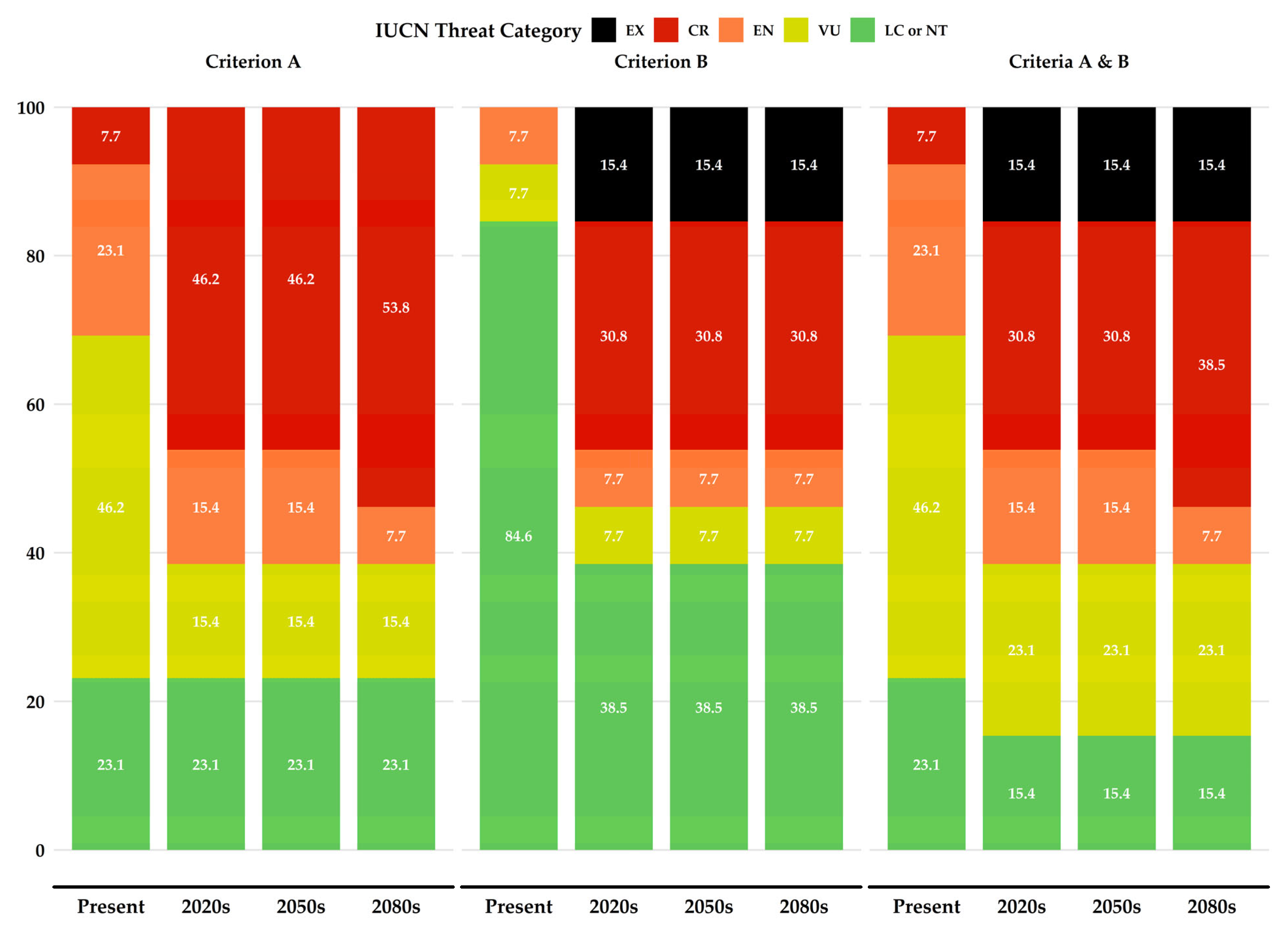
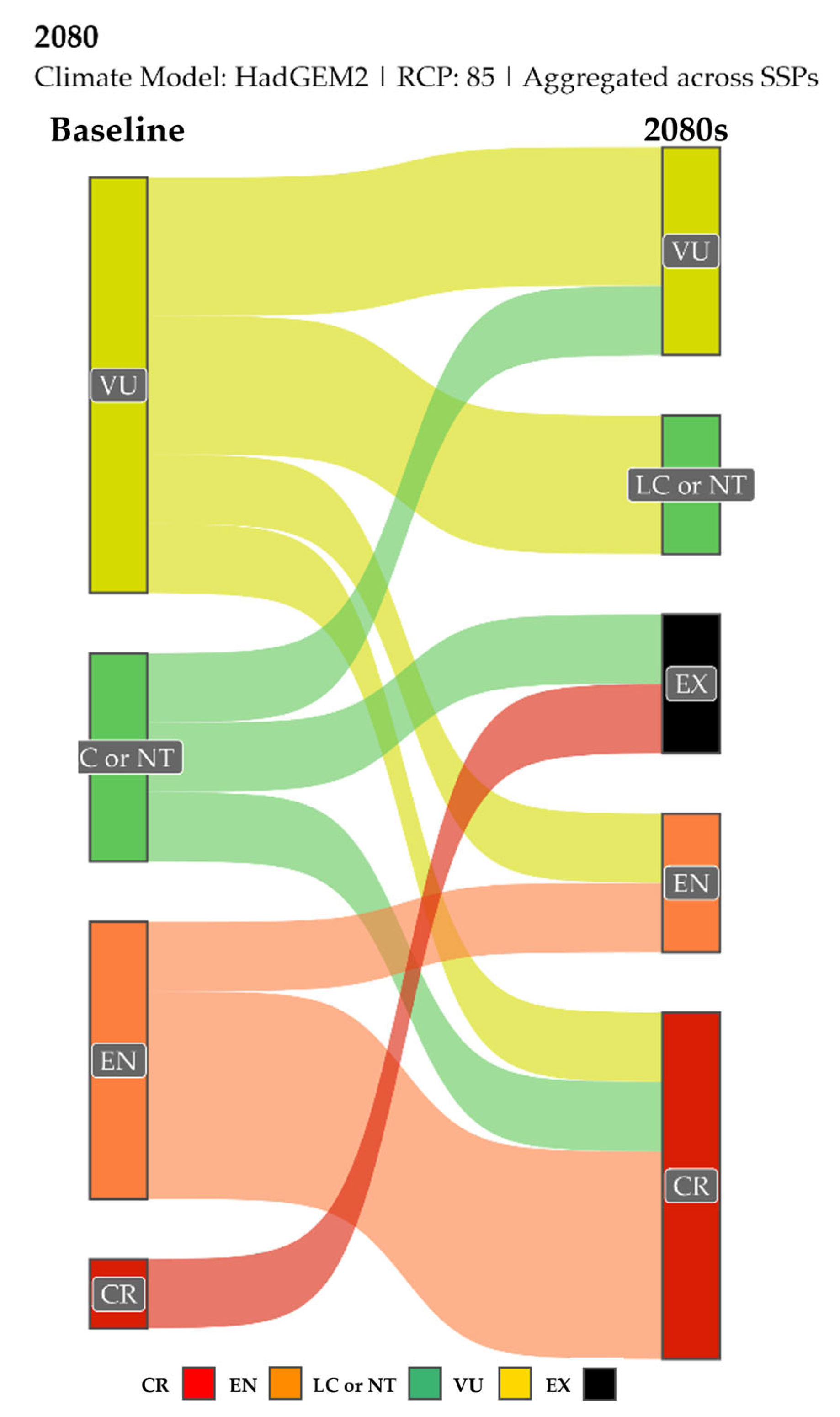
3.7. IUCN Extinction Risk Assessment

Our SDM-based extinction risk assessments for the baseline period showed complete concordance with the formal IUCN assessments for the five single-island endemics with existing evaluations. More specifically, the threat categories assigned based on our SDM projections corresponded with those determined by the IUCN for all five taxa (Table S11). This validation of our methodology against independent expert assessments strengthens the reliability of our projected future extinction risks under climate and land use change scenarios and indicates that our models effectively reflect the current distributions and extinction risks of these species.

Our analysis of Evvia’s single-island endemic species under IUCN Criterion A reveals that currently, 23.1% are classified as Least Concern (LC) or Near Threatened (NT; Table S12; Figure 9). This proportion remains consistent through to the 2080s (Table S12; Figure 9), indicating that these taxa may exhibit resilience in population size despite projected environmental changes. However, the percentage of species classified as Critically Endangered (CR) increases significantly, rising from 7.7% at present to 53.8% by the 2080s (Table S12; Figure 9). This sharp escalation suggests that many species are expected to experience severe population declines.

Under Criterion B, which assesses geographic range size, our projections show a concerning trend. The proportion of species deemed Extinct (EX) rises from zero currently to 15.4% by the 2020s and remains at this level thereafter (Table S12; Figure 9). This early increase indicates an immediate extinction risk for certain species within the next few years.

When we combine both Criteria A and B, the deterioration in conservation status becomes more pronounced. The percentage of species classified as CR or EX increases markedly from 7.7% at present to 53.9% by the 2080s (Table S12; Figure 9). Conversely, the proportion of species assessed as LC or NT decreases from 23.1% to 15.4% over the same period. These trends suggest a progressive decline in the overall conservation status of the single-island endemics in Evvia in the coming decades. Alyssum densistellatum and Viola dirphya are expected to become extinct under any GCM/RCP/SSP and period combination (Table S12).

Figure 10 shows the projected transitions between IUCN threat categories for the worst-case scenario HadGEM2 RCP 8.5 (aggregated across SSPs). While there is some variation across different GCMs and RCPs (see Supplementary Figures S38–S40 for all scenarios), the overall trend is consistent: a substantial proportion of species shift from lower to higher threat categories by the 2080s.

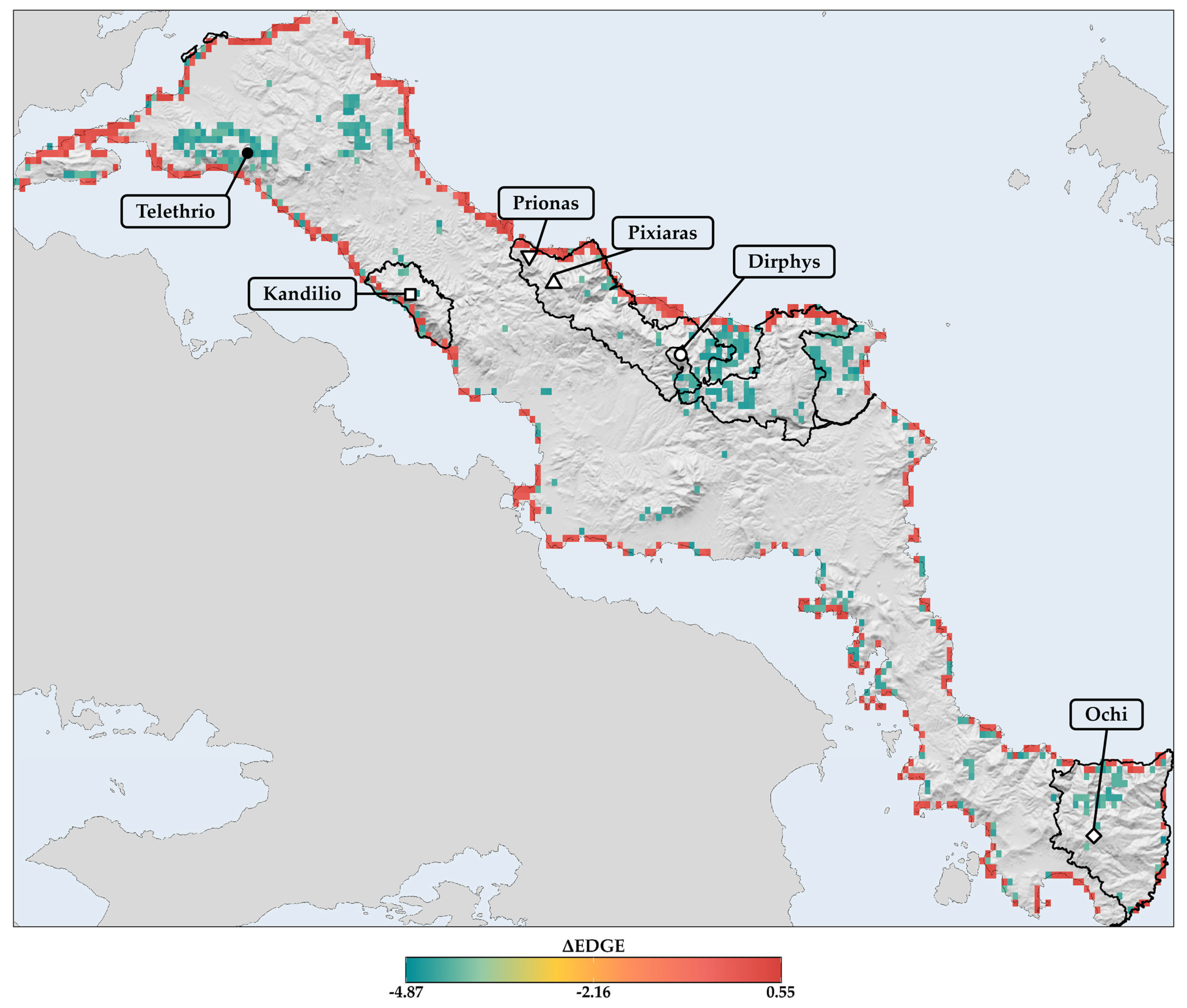
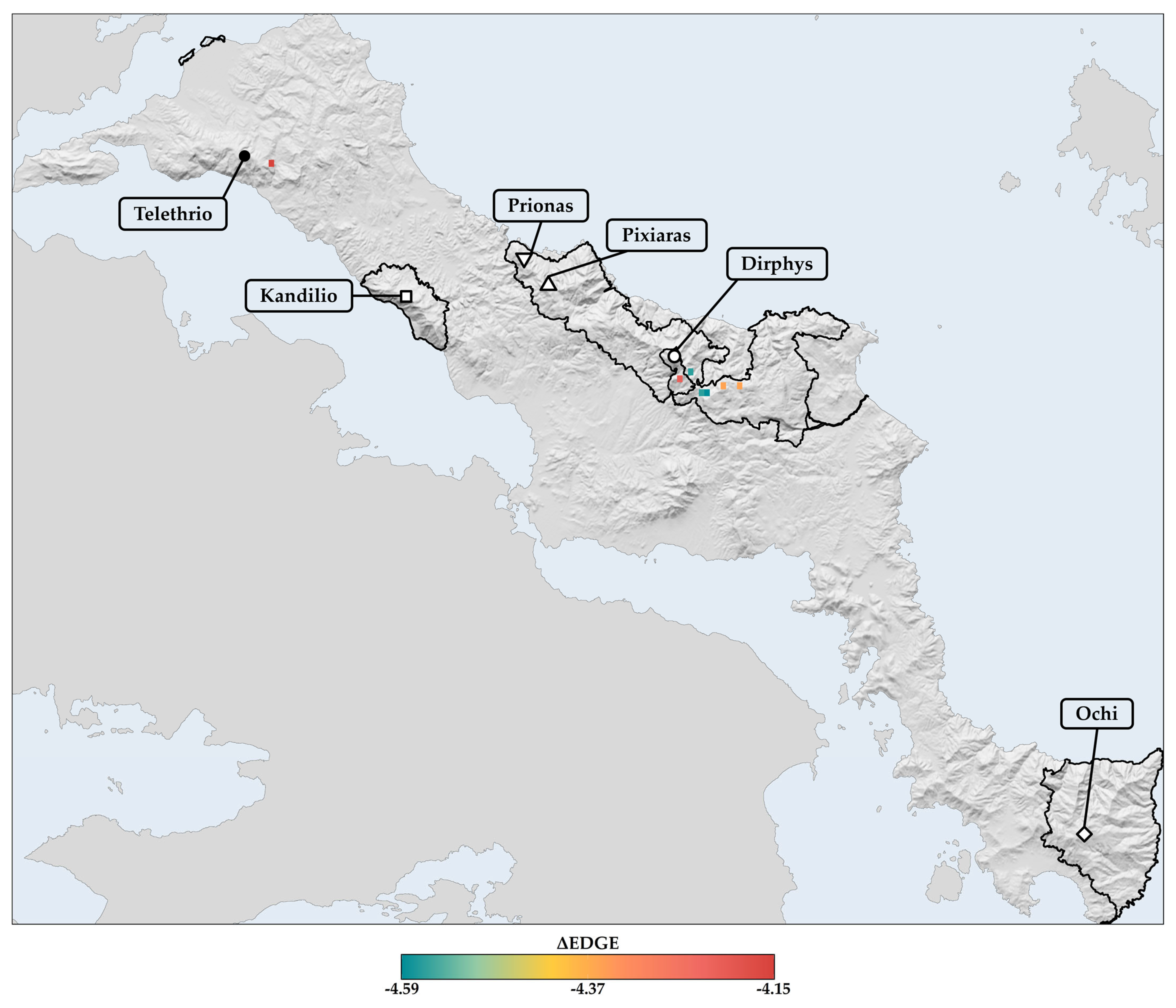
3.8. Estimation of the Evolutionarily Distinct and Globally Endangered (EDGE) Index—Current and Future EDGE Spatial Patterns

Based on Criteria A and B, the EDGE scores for single-island endemics range from 4.07 to 5.48, with a median of 4.48 (Tables S12 and S13). Only two taxa, namely Asperula suffruticosa and Viola dirphya, exhibit EDGE scores surpassing 5.0, with Viola dirphya being the sole species classified as CR.

The projected spatial patterns of the ΔEDGE index for the 2080s reveal a heterogeneous distribution of probable extinction hotspots and coldspots across Evvia, with these patterns being similar across periods (Sperman’s rho: 95.6–97.4%; Figure 11 and Figures S41 and S42). Most grid cells with negative ΔEDGE values are concentrated in the south, central, and north mountain regions of Evvia, indicating areas where evolutionarily distinct and threatened single-island endemics are at higher risk of extinction due to climate and land use change (Figure 11 and Figures S41 and S42). These probable extinction hotspots are especially evident in Mts. Dirphys and Telethrio, where they coincide with 14% of the CWE-PE L1 hotspots for single-island endemics (Figure 12), covering an area of 4.63 km². Among these overlapping grid cells, one located in Mt. Telethrio lies outside the Greek protected areas network in Evvia, representing a significant conservation gap as it constitutes both a hotspot of probable extinction for evolutionarily distinct and threatened single-island endemics and a L1 CWE-PE hotspot (Figure 12). Furthermore, numerous other grid cells with highly negative ΔEDGE values in northern and central Evia fall outside the Greek protected areas network (Figure 11). The spatial patterns accent the need for targeted conservation efforts in the identified extinction hotspots to reduce the impact of climate and land use change on evolutionarily distinct and threatened taxa in these regions.

4. Discussion

To map the distributions of 114 endemic plant taxa on Evvia (see Section 2), we used the ESM framework. This approach suits taxa with sparse occurrence records by merging predictions from simple bivariate models [59,104,107]. Unlike complex models that risk overfitting when trained on small samples [195], ESMs maintain accuracy through their ensemble structure. Though not immune to small-sample limitations [59], ESMs excel at discriminating between suitable and unsuitable habitats—our main objective—and thus provide robust projections of range changes under climate and land use scenarios [59]. Despite the limitations imposed by small sample sizes for some taxa, our model evaluation metrics indicate good to excellent discriminatory performance (Figure S1; Table S2). The models’ reliability gained additional support through complete agreement between our SDM-based extinction risk assessments and existing IUCN evaluations for five single-island endemics during the baseline period (see Section 4.2). Furthermore, our use of the Shape metric to quantify and address extrapolation uncertainty adds an additional layer of reliability to our projections, particularly for future scenarios (see Section 2.3).

Our study uncovers how climate and land use change may affect the endemic flora of Evvia, using a robust species distribution modelling approach that integrates both climate and land use change projections. We analysed a thorough set of environmental variables, including bioclimatic, topographical, soil, and land use data, to model the realised climatic niches of 114 endemic plant taxa (Table S2). Land use change projections were incorporated into the models by using dynamic land use data for both current and future scenarios. This integration of land use change alongside climate change projections strengthens the reliability and applicability of our findings.

Our results indicate the vulnerability of Evvia’s endemic flora to climate change, projecting substantial range contractions, increased habitat fragmentation, and altitudinal shifts. Biodiversity hotspots are projected to shift from mountainous areas to lowland regions, while coldspots will expand to higher elevations. Temporal beta diversity patterns suggest a future loss of distinct evolutionary lineages at higher altitudes and increased turnover in lowland areas. The magnitude and direction of these changes, however, vary considerably among taxa and are subject to multiple sources of uncertainty, including the limitations of presence-background data, the assumption of niche conservatism, the possible interactions with invasive species, pollinator dynamics, and microhabitat processes not fully captured in our models (see Section 4.6 for a detailed discussion). Nonetheless, it is important to note that unmodeled biotic interactions could alter these outcomes.

4.1. Species-Specific Responses to Global Change Drivers

Our findings indicate that all examined taxa are projected to experience range reductions, with median losses of 22.9% by the 2080s under the most severe climate scenario (HadGEM2 RCP 8.5 SSP1). Single-island endemics are particularly vulnerable, with a median projected range reduction of 63.2% in the 2080s, compared to 35.1% for Greek endemics (Tables S4–S6; Figure 2 and Figures S4–S6). More specifically, Alyssum densistellatum and Viola dirphya are expected to lose their entire suitable habitat, while Alyssum euboeum may maintain its current range (Tables S5 and S6; Figure 2 and Figure 3). These projections highlight the heightened sensitivity of narrowly distributed species to climate and land use changes [196].

The differential responses between Greek endemics and single-island endemics can be attributed to the distinct environmental factors influencing their distributions (Table S3; Figure S3). Greek endemics occurring in Evvia are primarily affected by Thornthwaite’s aridity index and their occurrence in grasslands and shrublands (Table S3; Figure S3), reflecting their adaptation to stable, dry, and rocky Mediterranean habitats [18,197]. Single-island endemics are more influenced by temperature/aridity-related factors and their occurrence in barren lands (Table S3; Figure S3), indicating a greater sensitivity to temperature fluctuations and heat stress, since most neo-endemics in Evvia occur in relatively arid areas with low climate change velocity [18].

The marked variation in projected range changes among both single-island endemics and Greek endemics on Evvia is also linked to species-specific associations with different land use types. Taxa restricted to areas classified as barren land—which are forecasted to contract considerably in the coming decades (Figures S33–S36)—face more severe range contractions (e.g., Alyssum densistellatum, Viola dirphya) compared to taxa occurring in other land use types as well (e.g., Cerastium candidissimum, Fritillaria euboeica). In contrast, species inhabiting land use types projected to remain stable or expand, such as forested areas or shrublands, show greater resilience, with some maintaining their current distributions or experiencing only minor range reductions (e.g., Abies cephalonica, Paeonia mascula subsp. hellenica, Malcolmia macrocalyx or some bulbous geophytes, such as Ornithogalum exaratum and Crocus laevigatus). Local afforestation and woody vegetation encroachment account for most of the observed net positive land use effects by enlarging forested and shrub-dominated habitats. These processes favour species reliant on understorey microhabitats or those requiring thorny shrub barriers to limit herbivory. Moreover, ongoing agricultural abandonment in parts of Evvia is expected to facilitate the conversion of croplands into woody vegetation formations [67]. This expansion partially offsets adverse climatic impacts by increasing the availability of suitable habitats for endemic taxa adapted to these vegetation types. This distinction underscores the importance of considering species-specific ecological requirements when assessing vulnerability to global change drivers and the interplay of ecological, evolutionary, and anthropogenic forces in shaping species distributions [198].

Our projections indicate increased habitat fragmentation and reduced connectivity for all taxa (Figure S8). Future fragmentation metrics show lower scores than current values, suggesting that the combined effects of climate and land use changes will exacerbate habitat isolation, consistent with the data reported for other rare Greek endemics occurring in mainland Greece [27,30]. This fragmentation poses additional challenges for species dispersal and gene flow, particularly for endemics with limited dispersal ability.

Habitat fragmentation, a major driver of biodiversity decline, may lead to increased extinction risk for numerous taxa by reducing habitat connectivity and increasing isolation [199]. This threat, according to a meta-analysis, is more pronounced in habitat specialists compared to generalists, since they might experience up to 35% higher extinction rates in fragmented landscapes [200] and, as a result, become even more susceptible to additional habitat degradation.

Comparative Analysis with Other Island Systems

Our analyses reveal broadly consistent patterns with those documented in various island systems (Table S14), demonstrating increased extinction risks for endemic species under climate change scenarios. Climate change models for Crete project a 98.3% range reduction for 172 single-island endemics, with up to 90% facing potential extinction within decades [28]. While our projections for the single-island endemics of Evvia are on par with those from Crete, the lower magnitude of projected range reductions on Evvia, compared to Crete, likely reflects both reduced anthropogenic pressure—characterised by lower rates of urban expansion and tourism development—and our incorporation of land use change variables. This methodological approach typically yields more conservative range decline and extinction risk projections, as evidenced across diverse taxa in Greek mainland endemics in the Peloponnese [27] or the entire Madagascar endemic flora [201].

This methodological distinction is exemplified by Nepeta argolica subsp. dirphya, where climate-only models once projected a 75.4% range contraction on Evvia [26], while our integrated assessment (factoring both climate and land use change) projects a much smaller 6% reduction. Such marked differences accentuate the value of evaluating multiple global change drivers simultaneously, revealing how land use alterations can modulate or, in some cases, exacerbate climate change impacts [27,33,201,202].

The vulnerability of island plants to global change extends far beyond the Mediterranean Basin. Studies across diverse island systems, such as the Canary Islands [22], Cabo Verde [203], Japan [204], Socotra [205], Madagascar [201], and the Falkland Islands [206], demonstrate consistent patterns of projected range reductions and potential extinctions for endemic plant taxa (Table S14). In particular, climate change models project range reductions of 38% for 228 single-island endemics in the Canary Islands and 74% for 469 single-island endemics in New Caledonia [22,24]. However, important differences in topography, land use intensity, and evolutionary histories may limit straightforward comparisons.

Our findings reveal the substantial vulnerability of Evvia’s endemic flora to climate and land use change, with projected habitat losses and fragmentation over the coming decades reflecting their demonstrated sensitivity to temperature fluctuations and heat stress (Table S3; Figure S3). These comparisons highlight a consistent trend of significant range contractions and extinction risks for endemic plant taxa across various Mediterranean and island ecosystems. The similar magnitudes of projected area loss and extinction rates emphasise that the challenges faced in Evvia are part of a broader global issue requiring coordinated conservation efforts, but regional-scale incentives and stakeholder engagement will shape practical outcomes.

This vulnerability is particularly acute in island ecosystems like Evvia, which function as extinction hotspots [7] where endemic species face disproportionate extinction risks [207]. While our projected extinction rates correspond with global estimates [12], we posit that these projections are conservative. This assessment is based on three key factors. First, SDMs incorporating dynamic land use variables typically underestimate local extirpations [208]. Second, potential extinction debts remain unaccounted for, arising from plants’ lagged responses to environmental change, extended life histories, and persistence in soil seed banks [209,210,211]. Third, our models exclude biotic interactions, particularly the cascading effects of pollinator network collapse [212] and consequent reproductive failure [213], factors especially pertinent in Evvia’s highlands, where pollinator Wallacean shortfalls exceed those of other Aegean islands and multiple pollinator extinctions are projected by the end of the century [214].

4.2. Extinction Risk Assessment

Our SDM-based extinction risk assessments for the baseline period showed complete concordance with formal IUCN assessments for the five previously evaluated single-island endemics (Table S12), validating our projections of future extinction risks under combined climate and land use change scenarios.

4.2.1. Projected Changes in Threat Categories

Threat assessment projections reveal critical trajectories for Evvia’s single-island endemics under all GCM/RCP/SSP and period combinations. Currently, while 23.1% of species are classified LC or NT under both Criteria A and B, this percentage will drop slightly, as the extinction risk status for at least two taxa (Campanula cymaea and Centaurea mantoudii) is projected to improve under all GCM/RCP/SSP and period combinations (Table S12). However, the proportion of CR species shows a dramatic increase from 7.7% at present to 38.5% by the 2080s under both Criteria, suggesting severe projected population declines and range contractions. Our results are in line with [215], who stated that up to 39–45.1% of all vascular plant species will be threatened with extinction over the coming decades, as well as with [216], who found that range contractions could lead to a deterioration of the threat assessment of some Italian plants.

Our findings parallel those of [217], who project 16–70% species extinction rates even with niche shifting capacity—a particularly challenging prospect for Evvia’s endemic perennial (sub-)shrubs. At least five single-island endemics, namely Asperula suffruticosa, Campanula constantinii, Quercus trojana subsp. euboica, Sideritis euboea, and Silene oligacantha subsp. pseudoradicosa, are projected to become classified as CR within the current decade (Table S12), necessitating immediate conservation intervention. This is especially worrying for Sideritis euboea. While a recent study on its Mt. Dirphys population [218] indicated relatively low genomic erosion linked to slower vegetation greening its Mt. Ochi subpopulations already exhibit genetic depletion under intense anthropogenic pressure [219], highlighting population-specific vulnerabilities.

Furthermore, the proportion of Extinct species will rise from zero at present to 15.4% by the 2020s under Criterion B and remain stable thereafter, indicating that some species (i.e., Alyssum densistellatum and Viola dirphya) may face imminent extinction within the next few years, as is the case for Allium iatrouinum [29]. Such a prospect is particularly alarming given that Criterion B evaluates geographic range size, a key consideration for island endemics with naturally restricted distributions.

4.2.2. Comparative Analyses with Other Island Endemics and Island Systems

Overall, our results indicate a progressive deterioration of conservation status over time, with CR or EX categories soaring from 7.7% to 53.9% by the 2080s and LC/NT species diminishing from 23.1% to 15.4%. Our findings parallel projections from Crete, the hottest Mediterranean island biodiversity hotspot [8], where up to 19 single-island endemics are projected to become extinct by the end of the century [28]. Similar extinction trajectories are projected for genetically depauperate single-island endemic taxa, such as Allium iatrouinum and Aethionema retsina [29] and even specialised coastal cliff Greek endemics with relative reproductive success, such as Limonium zacynthium or Asperula naufraga [220,221].

More specifically, Evvia exhibits higher extinction risks compared to two global island biodiversity hotspots (Table S14; Figure 9): the Canary Islands (4.39% extinction risk for 228 single-island endemics; [22]) and New Caledonia (15% extinction risk for 469 single-island endemics; [24]). Considering that both fragmentation metrics included in our analyses are expected to increase in the future, this fact stresses the vulnerability of Evvia’s endemic flora to climate and land use change, with substantial habitat losses and fragmentation expected over the coming decades, which reflects the Evvian single-island endemics’ sensitivity to temperature fluctuations and heat stress (Table S3; Figure S3).

These changes may accelerate genetic diversity erosion, which is particularly concerning given the already low genetic diversity and increased extinction risk among many Greek endemics [29,220,221,222,223]. Our findings support [18]’s hypothesis that increased extinction rates in Greece may reflect Greek endemics’ inability to track their realised niche shifts under changing climatic conditions.

The results of this study have immediate implications for conservation planning in Evvia. The projected rapid decline in species’ conservation status suggests that proactive conservation measures are needed rather than reactive management approaches. The stability in some threat categories after the 2020s might indicate the existence of potential climatic microrefugia in coastal precipitous cliffs that could serve as priority areas for conservation efforts.

Finally, it is possible that our model-based projections underestimate local extirpations if species experience lagged responses or if negative interactions (e.g., invasive species, pollinator declines) accelerate population declines. Further field-based research would help elucidate whether these worst-case scenarios unfold in the coming years.

4.3. Shifts in Biodiversity Hotspots

Our analyses identified a significant concentration of endemic taxa in mountainous regions on Evvia (Figures S9–S16)—a trend that has also been reported across other areas [224]. This clustering is often tied to the increased isolation and diverse range of habitats found in these rugged landscapes [225], as mountain systems function as both historical refugia and centres of speciation, with their topographical complexity creating distinct microclimates and ecological niches that promote species diversification [226]. Mediterranean mountain ranges typically exhibit higher endemism rates compared to lowland areas, partly due to their role as climatic buffers during past environmental fluctuations [16] and their capacity to maintain isolated populations through topographic barriers [227]. Greek endemics occurring in Evvia are distinguished by their limited distribution ranges and specialised habitat requirements [31,32], with many occurring exclusively in challenging environments such as cliffs and screes [228,229,230].

4.3.1. Projected Spatial and Altitudinal Redistributions

The results of this study reveal substantial spatial and altitudinal redistributions of the Greek endemic plants occurring in Evvia, especially for the single-island endemics. Currently identified Priority Hotspots face significant altitudinal contractions, with projected altitudinal losses of 56.2–93.4% affecting 42.4% of their extent (Table S7; Figure 4 and Figures S17 and S22). Such drastic reductions threaten irreplaceable plant genetic repositories, calling for urgent, proactive management actions [231,232].

Currently established mountainous hotspots (Figure 4, Figure 5, Figure 6 and Figures S17, S27 and S28), including Mt. Dirphys, are projected to lose their conservation significance, while new hotspots will emerge in lowland and coastal regions (Figure 5 and Figure S27). This trend, rather than reflecting a genuine surge in endemism at lower altitude, more likely signifies a redistribution sparked by differential taxonomic losses across elevational gradients. Most Greek endemics occurring in Evvia and all the single-island endemics are projected to lose a significant portion of their altitudinal range (Figure S22), conforming to the documented patterns of altitudinal range contractions [233]. Only a few might be able to track their niche upwards as a response to increasing aridity [234], probably due to the escalator to extinction effect [235], since mountainous island species are especially vulnerable to global change drivers due to their limited dispersal capacity and the finite nature of upslope habitat [236]. Any projected downslope range shifts may be attributable to competitive release, habitat modification, or the combination of both processes [237].

4.3.2. Evolutionary Implications and Future Refugia

Maximum taxonomic and phylogenetic temporal turnover is projected for lowland regions (Figure 8 and Figure S31), especially for the single-island endemics, indicating a substantial restructuring of species compositions and evolutionary histories. Climate and land use changes are likewise expected to drive lineage loss in mountainous areas while favouring more stress-tolerant or generalist taxa in lowlands. The EHSA analyses support this trend, as various lowland and coastal areas emerge as new hotspots, while several high-altitude areas appear as sporadic hotspots (Figure 7 and Figure S29).

This dynamic reorganisation of species and communities may foster biotic homogenisation [238], challenging the spatial stability of biodiversity hotspots in the Anthropocene [239]. Future refinements in community-level models should also account for complex species interactions that may modulate or exacerbate these transitions. Our findings demonstrate that climate and land use change may fundamentally reshape biogeographic patterns at local scales, consistent with observations across multiple biodiversity hotspots and taxa [28,30,163,214,240,241].

These apparent shifts in biodiversity hotspot distribution do not necessarily imply that new areas are gaining endemic species. More likely, they reflect a decline in endemic taxa within existing hotspots, which subsequently creates a proportional increase in other regions. Because CWE and PE (measures that emphasise rarer and evolutionarily distinct taxa) are especially sensitive to the loss of evolutionarily distinct taxa with limited ranges, the disappearance of these taxa in certain hotspots can artificially raise CWE and PE values in areas where at least some of those taxa remain. If generalist, closely related taxa prove more resilient to changing conditions, the overall result can be higher CWE and PE values—even in the face of declining total biodiversity.

Future hotspot convergence—at least in some mountainous areas—for Greek endemic taxa and Evvian single-island endemics—despite current distributional differences (Figures S9, S13, S18, S20 and S23–S26)—suggests potential shared refugia for resilient taxa (e.g., Alyssum euboeum or Campanula euboica), particularly in northeastern and central Evvian coastal cliffs. Many Greek endemics occurring in Evvia possess stress-tolerance strategies [32] and are either obligate or facultative cliff endemic chasmophytes [228,229].

Chasmophytic cliff endemics exhibit higher survival rates which may be attributed to their physiological adaptations, the higher expression of genes regulating oxidative phosphorylation, and their life-history traits, as cliff endemics are high-stress-tolerant plants [10,242,243]. In the Aegean, precipitous coastal cliffs harbour a highly specialised and often relictual endemic flora (ca. 21% of the Greek endemics; [228,229]) of Messinian origin [244,245]. These taxa have persisted through random genetic drift and microclimatic buffering despite progressive climatic deterioration over the last 5 My [244,245]. Thus, the coastal cliff areas where future biodiversity may lie could host the more stress-tolerant endemic taxa, those who might be able to withstand the intense climate and land use change impacts due to their innate resilience.

This potential for shared refugia has significant implications for conservation planning, as it necessitates the development of strategies that can accommodate multiple taxa with likely divergent ecological requirements. However, we have to note that we did not explicitly consider the adaptive capacities of endemic species [246], which may influence their long-term responses to global change. While there is evidence of rapid evolution and phenotypic plasticity in some island plants [247,248,249], empirical data on the adaptive potential of Evvia’s endemic flora is currently lacking. Uncertainties concerning pollinator availability, seed bank persistence, and propensity for dispersal further compound the predictive limitations. Future research should investigate the genetic diversity and adaptive capacities of these species through field studies, common garden experiments, and genetic analyses to refine our understanding of their vulnerability to climate and land use change [29,222].

4.3.3. Conservation Priorities

The high-altitude regions, despite functioning as current diversity and conservation hotspots with increased EDGE scores (Figure 11 and Figures S41 and S42), risk transitioning into extinction hotspots, as indicated by their low ΔEDGE scores (Figure 11 and Figure 12). This worrisome pattern, also noted in Crete [28], appears especially pronounced in Mts. Dirphys and Telethrio, where these potential extinction hotspots overlap with 14% of the CWE-PE L1 hotspots identified for single-island endemic species (Figure 11). Additional areas exhibiting very low ΔEDGE scores are found in northern and central Evvia, falling outside the established protected areas network (Figure 12).

These vulnerable regions warrant urgent prioritisation in conservation initiatives. The imperative to identify conservation priorities and implement efficient measures grows increasingly pressing as human activities and land use exert unrelenting pressure on natural habitats, precipitating severe alterations in biodiversity [3,202]. The strategic identification of areas characterised by high EDGE and low ΔEDGE scores offers a robust, data-driven approach for prioritising regions of high conservation and evolutionary significance that face increased extinction risk, as demonstrated in Crete [28]. Adopting this approach can inform the development of targeted, evidence-based conservation strategies to protect biodiversity in the face of unprecedented anthropogenic pressures. Given Evvia’s exposure to repeated wildfires and infrastructure expansion (e.g., wind farms), further habitat degradation could amplify extinction risks unless integrated management plans are implemented.

4.4. Effectiveness of Protected Areas and Conservation Gaps

The Natura 2000 protected area network in Evvia is projected to become less effective at preserving shifting patterns of endemic diversity, which compels a re-evaluation of current conservation priorities. Concurrent LULC changes, such as the expansion of shrublands and forests and the abandonment of croplands, may present both opportunities and challenges for the endemic taxa. While presently a high percentage of hotspots are within NATURA 2000 sites, this coverage is projected to decline over time—to as low as 36.9% for Greek endemics and 8.8% for single-island endemics (Tables S8–S10), in line with previous studies from Greece and other regions across the globe [27,28,214,250,251,252,253]. These patterns are further exemplified by the spatial variability identified through the Emerging Hot Spot Analysis, which highlights dynamic shifts in hotspots across time, including areas with inconsistent or sporadic protection (Tables S9–S11).

Such coverage losses expose critical conservation gaps, emphasising that static protected-area boundaries may fail to capture rapidly shifting biodiversity patterns [254]. The projected decline in the coverage of current Priority Hotspots by protected areas (Tables S7, S9, and S10) indicates that conservation strategies should be adaptive and regularly updated to accommodate changing species distributions. More specifically, while current conservation efforts in Evvia may appear sufficient based on present species distributions, the anticipated future shortfalls—ranging from moderate declines in coverage to near-complete gaps—highlight the urgent need to reevaluate the design and management of protected areas [254], as suggested in previous studies [18,20,214,255,256]. This could involve the implementation of flexible protected area networks or the prioritisation of future biodiversity hotspots in land use planning. Specifically, we recommend the following actions for Evvia, in line with the EU Biodiversity Strategy for 2030 and the post-2020 global biodiversity framework:

(a)

Identify and prioritise areas projected to serve as future biodiversity hotspots for legal protection and conservation management, contributing to the EU’s target of protecting 30% of land and sea by 2030.

(b)

Develop iterative conservation plans that can accommodate shifts in species distributions and ecological requirements over time, ensuring the long-term effectiveness of protected areas.

(c)

Engage local communities and stakeholders in conservation planning efforts to ensure that socio-economic considerations are addressed, promoting the integration of biodiversity values and ecosystem services into local planning and development processes.

(d)

Strengthen monitoring programmes to track changes in species abundances and distributions, informing adaptive management strategies and contributing to the EU’s goal of improving knowledge, the science base, and technologies relating to biodiversity, relevant ecosystem services and natural capital accounting.

Implementing these recommendations will require close collaboration among researchers, conservation practitioners, policymakers, and local communities. The possible socio-economic impacts of the projected biodiversity changes, such as the loss of ecosystem services and/or unique critical natural capital elements or the need for a direct turn to more sustainable land use practices, should be carefully considered in conservation planning efforts. By linking conservation goals with sustainable development objectives, such as the UN Sustainable Development Goals, Evvia can serve as a model for integrating biodiversity conservation into broader societal goals.

It is important to acknowledge that our study focused primarily on the direct impacts of climate and land use change on endemic plant distributions. However, other anthropogenic stressors, such as pollution, invasive species, and habitat fragmentation, may also interact with these drivers to shape future biodiversity patterns. For example, the increasing frequency and intensity of wildfires on Evvia, exacerbated by climate change and land use practices, could accelerate habitat loss and fragmentation for endemic species. Similarly, the expansion of invasive plant species, facilitated by climate change and human activities, could increase competition and further restrict the suitable habitat for endemic taxa. Future research should aim to integrate these additional stressors into species distribution models and conservation planning efforts to provide an in-depth understanding of the threats facing Evvia’s biodiversity.

4.5. Management Implications

In this study, we documented the climate and land use change impact on the endemic flora of Evvia, an impact that acts incrementally with changes caused by wildfires and the development of wind farms, due to habitat loss, degradation, alteration, and possible ecological disruption. The construction and operation of wind farms can lead to habitat fragmentation, which may adversely affect narrowly distributed species like those found at the higher altitudes of Evvia’s mountains. Additionally, fires (like the 2021 Evvia megafire), whether natural or anthropogenic, can further exacerbate these threats by altering the delicate balance of these ecosystems, likely leading to the loss of endemic species that are not adapted to frequent fire disturbances. While the development of wind farms on Evvia could contribute to sustainable energy goals, it is imperative to balance these developments with the conservation of the island’s unique endemic flora, considering the present study’s findings on climate–land use change impact. The provisions of the EU Green Deal and the recently adopted EU Nature Restoration Law should guide future actions and draft a prioritisation scheme for the different ecosystems and habitat types towards resilience in future conditions.

Therefore, to protect the local endemic plant taxa from climate change, land use alteration, and the possibility of repetitive forest fires, a multifaceted approach is necessary, integrating habitat management, conservation genetics, and fire management strategies.

Firstly, understanding the potential impacts of climate change on habitat suitability is vital. SDMs have shown that many Greek tree species may experience habitat shrinkage under future climate scenarios, particularly at higher elevations. However, some species, such as Abies cephalonica, may maintain their distribution under certain scenarios, suggesting that targeted conservation efforts could reduce some impacts of climate change [257]. For endemic medicinal and aromatic plants, such as those in the genus Nepeta, SDMs predict severe range retractions due to climate change, driven by soil and aridity variables. Conservation efforts should focus on identifying and protecting current and future species richness hotspots, which are expected to shift geographically over time [26].

Fire management is another critical component. High-altitude coniferous forests, including those dominated by Greek fir (Abies cephalonica) and black pine (Pinus nigra), are increasingly affected by fires, which these species are not adapted to regenerate from naturally. Active reforestation and careful management of fire-prone regions are necessary to aid in tree recovery and maintain ecosystem integrity [258], as well as for in situ and ex situ conservation actions. Additionally, conservation genetics can play a vital role. For CR Greek endemics, genetic diversity assessments reveal moderate diversity levels, indicating possible resilience to environmental changes. However, climate change is expected to significantly impact their range sizes. In situ measures, such as population reinforcement, and ex situ strategies, like seed bank conservation, are recommended to preserve genetic diversity and ensure long-term survival [29].

4.6. Limitations and Uncertainties

Our analyses of climate and land use change effects on Evvia’s endemic flora face several methodological constraints. The sparse occurrence records for many taxa introduce uncertainty in SDMs, which can lead to both the under- and overestimation of suitable habitats. Although the ESM framework helps address these issues, the fundamental constraints of small-sample modelling persist. The use of presence-background data, rather than presence–absence information, limits our models to estimating relative habitat suitability instead of true occurrence probability. Model performance varies with background point selection and the thresholds used for converting continuous suitability scores to binary predictions. Moreover, our models rest on the assumption that species–environment relationships remain static over time. This premise might not hold if species adapt to environmental changes, species interactions shift, or current distributions are not at equilibrium. Similarly, we assumed minimal dispersal for all taxa. While this simplification suits many island endemics, some species possess dispersal abilities that could affect their future distributions. Furthermore, the models exclude biotic interactions such as interspecific competition, pollinator relationships, and herbivory, which shape species distributions and their responses to climate change. We also acknowledge that our models do not account for invasive species dynamics.

In our modelling framework, we incorporated static variables for topography and soil characteristics, based on the premise that these landscape features maintain relative stability over the temporal extent of our species occurrence dataset. This methodological choice reflects a standard practice in SDMs, primarily due to constraints in data availability. While temporally resolved datasets for certain soil processes exist—such as the global soil erosion estimates available through the European Soil Data Centre—their temporal and spatial resolutions often do not correspond to climate and species occurrence data. Using such mismatched datasets in SDM frameworks would introduce additional uncertainties and violate assumptions about temporal concordance amongst predictor variables. The decision to use static landscape variables likely has minimal impact on our findings for the taxa examined. The species in our study do not substantially modify soil properties or topography through their activities, nor do they predominantly occur in areas with high erosion rates within the study region. However, we recognise that future species distributions might be affected by localised changes in soil properties and topography, particularly in areas subject to climate change-induced erosion or intensive land use practices. As higher-resolution temporal datasets for landscape features become available, subsequent research could improve distribution forecasts for species that show sensitivity to these environmental changes. The use of static variables in SDMs requires careful consideration, as their disproportionate representation can artificially amplify their perceived importance and affect interpretations of habitat suitability [259,260]. Regarding the Greek endemics occurring on Evvia, topographical and soil parameters remain valid predictors, with their inclusion leading to high model precision and accuracy. However, the predictive strength of these static variables warrants cautious interpretation due to their tendency to show inflated importance in SDMs. While temporally static variables can limit model transferability across space and time, our thorough evaluation of extrapolation risks supports the reliability of our results. Our methodological framework demonstrated reduced uncertainty from both extrapolation and niche truncation [261,262], thus strengthening the model’s transferability. Finally, our projections reflect possible range changes under specific scenarios rather than definitive predictions. Species responses depend on numerous interacting factors that defy precise modelling. Thus, these results should form just one component of broader conservation planning and decision-making processes.

5. Conclusions

Our study assesses the potential impacts of climate and land use change on the endemic flora of Evvia, revealing complex patterns of range shifts, biodiversity hotspot reorganisation, and challenges to current conservation strategies. As global change accelerates, such integrated assessments—incorporating land use patterns, climate projections, and future adaptive responses—are necessary to devise robust, forward-looking conservation measures. The anticipated hotspot shifts from mountainous to lowland areas demonstrate that island conservation approaches require fundamental restructuring. By embracing dynamic, adaptive approaches and considering the complex interactions between multiple global change drivers, we can improve our ability to preserve the unique and irreplaceable biodiversity of island ecosystems in the face of unprecedented environmental change Future research should focus on:

• Incorporating biotic interactions and species’ adaptive capacities into modelling efforts
• Investigating the possibility for rapid evolution in island endemic plants in response to climate change
• Testing adaptive, long-term conservation strategies, such as flexible protected area designs and adaptive management approaches
• Assessing the implications of changing endemic plant distributions on ecosystem services

The current state of global biodiversity places island-endemic species at risk, with those on Evvia exemplifying broader challenges faced by other island ecosystems. Research findings should now translate into immediate, practical conservation measures to protect these irreplaceable island taxa and their habitats.

References

1. Watson, R.; Baste, I.; Larigauderie, A.; Leadley, P.; Pascual, U.; Baptiste, B.; Demissew, S.; Dziba, L.; Erpul, G.; Fazel, A. Summary for Policymakers of the Global Assessment Report on Biodiversity and Ecosystem Services of the Intergovernmental Science—Policy Platform on Biodiversity and Ecosystem Services; IPBES Secretariat: Bonn, Germany, 2019; pp. 22–47. [Google Scholar]
2. Moreira, H.; Kuipers, K.J.J.; Posthuma, L.; Zijp, M.C.; Hauck, M.; Huijbregts, M.A.J.; Schipper, A.M. Threats of Land Use to the Global Diversity of Vascular Plants. Divers. Distrib. 2023, 29, 688–697. [Google Scholar] [CrossRef]
3. Oliver, T.H.; Morecroft, M.D. Interactions between Climate Change and Land Use Change on Biodiversity: Attribution Problems, Risks, and Opportunities. Wiley Interdiscip. Rev. Clim. Change 2014, 5, 317–335. [Google Scholar] [CrossRef]
4. Newbold, T.; Oppenheimer, P.; Etard, A.; Williams, J.J. Tropical and Mediterranean Biodiversity Is Disproportionately Sensitive to Land-Use and Climate Change. Nat. Ecol. Evol. 2020, 4, 1630–1638. [Google Scholar] [CrossRef] [PubMed]
5. Poniatowski, D.; Beckmann, C.; Löffler, F.; Münsch, T.; Helbing, F.; Samways, M.J.; Fartmann, T. Relative Impacts of Land-Use and Climate Change on Grasshopper Range Shifts Have Changed over Time. Glob. Ecol. Biogeogr. 2020, 29, 2190–2202. [Google Scholar] [CrossRef]
6. Kehoe, R.; Frago, E.; Sanders, D. Cascading Extinctions as a Hidden Driver of Insect Decline. Ecol. Entomol. 2021, 46, 743–756. [Google Scholar] [CrossRef]
7. Fernández-Palacios, J.M.; Kreft, H.; Irl, S.D.H.; Norder, S.; Ah-Peng, C.; Borges, P.A.V.; Burns, K.C.; de Nascimento, L.; Meyer, J.-Y.; Montes, E. Scientists’ Warning—The Outstanding Biodiversity of Islands Is in Peril. Glob. Ecol. Conserv. 2021, 31, e01847. [Google Scholar] [CrossRef]
8. Médail, F. The Specific Vulnerability of Plant Biodiversity and Vegetation on Mediterranean Islands in the Face of Global Change. Reg. Environ. Change 2017, 17, 1775–1790. [Google Scholar] [CrossRef]
9. Lazoglou, G.; Papadopoulos-Zachos, A.; Georgiades, P.; Zittis, G.; Velikou, K.; Manios, E.M.; Anagnostopoulou, C. Identification of Climate Change Hotspots in the Mediterranean. Sci. Rep. 2024, 14, 29817. [Google Scholar] [CrossRef]
10. Thompson, J.D. Plant Evolution in the Mediterranean: Insights for Conservation; Oxford University Press: New York, NY, USA, 2020. [Google Scholar]
11. Urban, M.C. Climate Change Extinctions. Science 2024, 386, 1123–1128. [Google Scholar] [CrossRef]
12. Wiens, J.J.; Zelinka, J. How Many Species Will Earth Lose to Climate Change? Glob. Change Biol. 2024, 30, e17125. [Google Scholar] [CrossRef]
13. Asamoah, E.F.; Beaumont, L.J.; Maina, J.M. Climate and Land-Use Changes Reduce the Benefits of Terrestrial Protected Areas. Nat. Clim. Change 2021, 11, 1105–1110. [Google Scholar] [CrossRef]
14. Cao, Y.; Tseng, T.-H.; Wang, F.; Jacobson, A.; Yu, L.; Zhao, J.; Carver, S.; Locke, H.; Zhao, Z.; Yang, R. Potential Wilderness Loss Could Undermine the Post-2020 Global Biodiversity Framework. Biol. Conserv. 2022, 275, 109753. [Google Scholar] [CrossRef]
15. Cañadas, E.M.; Fenu, G.; Peñas, J.; Lorite, J.; Mattana, E.; Bacchetta, G. Hotspots within Hotspots: Endemic Plant Richness, Environmental Drivers, and Implications for Conservation. Biol. Conserv. 2014, 170, 282–291. [Google Scholar] [CrossRef]
16. Médail, F.; Diadema, K. Glacial Refugia Influence Plant Diversity Patterns in the Mediterranean Basin. J. Biogeogr. 2009, 36, 1333–1345. [Google Scholar] [CrossRef]
17. Hammoud, C.; Kougioumoutzis, K.; Rijsdijk, K.F.; Simaiakis, S.M.; Norder, S.J.; Foufopoulos, J.; Georgopoulou, E.; Van Loon, E.E. Past Connections with the Mainland Structure Patterns of Insular Species Richness in a Continental-shelf Archipelago (Aegean Sea, Greece). Ecol. Evol. 2021, 11, 5441–5458. [Google Scholar] [CrossRef]
18. Kougioumoutzis, K.; Kokkoris, I.P.; Panitsa, M.; Kallimanis, A.; Strid, A.; Dimopoulos, P. Plant Endemism Centres and Biodiversity Hotspots in Greece. Biology 2021, 10, 72. [Google Scholar] [CrossRef]
19. Panitsa, M.; Kagiampaki, A.; Kougioumoutzis, K. Plant Diversity and Biogeography of the Aegean Archipelago: A New Synthesis. In Biogeography and Biodiversity of the Aegean: In honour of Prof. Moysis Mylonas; Sfenthourakis, S., Pafilis, P., Parmakelis, A., Poulakakis, N., Triantis, K.A., Eds.; Broken Hill Publishers Ltd.: Nicosia, Cyprus, 2018; pp. 223–244. ISBN 9789925563784. [Google Scholar]
20. Kougioumoutzis, K.; Kokkoris, I.P.; Panitsa, M.; Strid, A.; Dimopoulos, P. Extinction Risk Assessment of the Greek Endemic Flora. Biology 2021, 10, 195. [Google Scholar] [CrossRef]
21. Benavides, E.; Sadler, J.; Graham, L.; Matthews, T.J. Species Distribution Models and Island Biogeography: Challenges and Prospects. Glob. Ecol. Conserv. 2024, 51, e02943. [Google Scholar] [CrossRef]
22. Hanz, D.M.; Cutts, V.; Barajas-Barbosa, M.P.; Algar, A.; Beierkuhnlein, C.; Collart, F.; Fernández-Palacios, J.M.; Field, R.; Karger, D.N.; Kienle, D.R.; et al. Effects of Climate Change on the Distribution of Plant Species and Plant Functional Strategies on the Canary Islands. Divers. Distrib. 2023, 29, 1157–1171. [Google Scholar] [CrossRef]
23. Fortini, L.B.; Price, J.; Jacobi, J.; Vorsino, A.; Burgett, J.; Brinck, K.W.; Amidon, F.; Miller, S.; Koob, G.; Paxton, E.H. A Landscape-Based Assessment of Climate Change Vulnerability for All Native Hawaiian Plants; University of Hawaii: Honolulu, HI, USA, 2013. [Google Scholar]
24. Pouteau, R.; Birnbaum, P. Island Biodiversity Hotspots Are Getting Hotter: Vulnerability of Tree Species to Climate Change in New Caledonia. Biol. Conserv. 2016, 201, 111–119. [Google Scholar] [CrossRef]
25. Kougioumoutzis, K.; Valli, A.T.; Georgopoulou, E.; Simaiakis, S.M.; Triantis, K.A.; Trigas, P. Network Biogeography of a Complex Island System: The Aegean Archipelago Revisited. J. Biogeogr. 2017, 44, 651–660. [Google Scholar] [CrossRef]
26. Kougioumoutzis, K.; Papanikolaou, A.; Kokkoris, I.P.; Strid, A.; Dimopoulos, P.; Panitsa, M. Climate Change Impacts and Extinction Risk Assessment of Nepeta Representatives (Lamiaceae) in Greece. Sustainability 2022, 14, 4269. [Google Scholar] [CrossRef]
27. Pires, M.B.; Kougioumoutzis, K.; Norder, S.; Dimopoulos, P.; Strid, A.; Panitsa, M. The Future of Plant Diversity within a Mediterranean Endemism Centre: Modelling the Synergistic Effects of Climate and Land-Use Change in Peloponnese, Greece. Sci. Total Environ. 2024, 947, 174622. [Google Scholar]
28. Kougioumoutzis, K.; Kokkoris, I.P.; Panitsa, M.; Trigas, P.; Strid, A.; Dimopoulos, P. Plant Diversity Patterns and Conservation Implications under Climate-Change Scenarios in the Mediterranean: The Case of Crete (Aegean, Greece). Diversity 2020, 12, 270. [Google Scholar] [CrossRef]
29. Kougioumoutzis, K.; Kotsakiozi, P.; Stathi, E.; Trigas, P.; Parmakelis, A. Conservation Genetics of Four Critically Endangered Greek Endemic Plants: A Preliminary Assessment. Diversity 2021, 13, 152. [Google Scholar] [CrossRef]
30. Kougioumoutzis, K.; Tsakiri, M.; Kokkoris, I.P.; Trigas, P.; Iatrou, G.; Lamari, F.N.; Tzanoudakis, D.; Koumoutsou, E.; Dimopoulos, P.; Strid, A. Assessing the Vulnerability of Medicinal and Aromatic Plants to Climate and Land-Use Changes in a Mediterranean Biodiversity Hotspot. Land 2024, 13, 133. [Google Scholar] [CrossRef]
31. Trigas, P.; Iatrou, G. The Local Endemic Flora of Evvia (W Aegean, Greece). Willdenowia 2006, 36, 257. [Google Scholar] [CrossRef]
32. Trigas, P.; Iatrou, G.; Panitsa, M. Vascular Plant Species Diversity, Biogeography and Vulnerability in the Aegean Islands as Exemplified by Evvia Island (W Aegean, Greece). Fresenius Environ. Bull. 2008, 17, 48–57. [Google Scholar]
33. Santos, M.J.; Smith, A.B.; Dekker, S.C.; Eppinga, M.B.; Leitão, P.J.; Moreno-Mateos, D.; Morueta-Holme, N.; Ruggeri, M. The Role of Land Use and Land Cover Change in Climate Change Vulnerability Assessments of Biodiversity: A Systematic Review. Landsc. Ecol. 2021, 36, 3367–3382. [Google Scholar] [CrossRef]
34. Dimopoulos, P.; Raus, T.; Bergmeier, E.; Constantinidis, T.; Iatrou, G.; Kokkini, S.; Strid, A.; Tzanoudakis, D. Vascular Plants of Greece: An Annotated Checklist. Englera 2013, 1–372. [Google Scholar]
35. Dimopoulos, P.; Raus, T.; Bergmeier, E.; Constantinidis, T.; Iatrou, G.; Kokkini, S.; Strid, A.; Tzanoudakis, D. Vascular Plants of Greece: An Annotated Checklist. Supplement. Willdenowia 2016, 46, 301–347. [Google Scholar] [CrossRef]
36. Dauby, G.; Stévart, T.; Droissart, V.; Cosiaux, A.; Deblauwe, V.; Simo-Droissart, M.; Sosef, M.S.M.; Lowry, P.P.; Schatz, G.E.; Gereau, R.E.; et al. ConR: An R Package to Assist Large-Scale Multispecies Preliminary Conservation Assessments Using Distribution Data. Ecol. Evol. 2017, 7, 11292–11303. [Google Scholar] [CrossRef] [PubMed]
37. Burgman, M.A.; Fox, J.C. Bias in Species Range Estimates from Minimum Convex Polygons: Implications for Conservation and Options for Improved Planning; Cambridge University Press: Cambridge, UK, 2003; Volume 6, pp. 19–28. [Google Scholar]
38. Jetz, W.; Sekercioglu, C.H.; Watson, J.E. Ecological Correlates and Conservation Implications of Overestimating Species Geographic Ranges. Conserv. Biol. 2008, 22, 110–119. [Google Scholar] [CrossRef]
39. Meyer, L.; Diniz-Filho, J.A.F.; Lohmann, L.G. A Comparison of Hull Methods for Estimating Species Ranges and Richness Maps. Plant Ecol. Divers. 2017, 10, 389–401. [Google Scholar] [CrossRef]
40. Zizka, A.; Silvestro, D.; Andermann, T.; Azevedo, J.; Duarte Ritter, C.; Edler, D.; Farooq, H.; Herdean, A.; Ariza, M.; Scharn, R. CoordinateCleaner: Standardized Cleaning of Occurrence Records from Biological Collection Databases. Methods Ecol. Evol. 2019, 10, 744–751. [Google Scholar] [CrossRef]
41. Smith, A.B. enmSdm: Tools for Modeling Species Niches and Distributions. R Package Version 0.5.1.5. 2020. Available online: http://github.com/adamlilith/enmSdm (accessed on 6 March 2025).
42. Lamboley, Q.; Fourcade, Y. No Optimal Spatial Filtering Distance for Mitigating Sampling Bias in Ecological Niche Models. J. Biogeogr. 2024, 51, 1783–1794. [Google Scholar] [CrossRef]
43. Ten Caten, C.; Dallas, T. Thinning Occurrence Points Does Not Improve Species Distribution Model Performance. Ecosphere 2023, 14, e4703. [Google Scholar] [CrossRef]
44. Baker, D.J.; Maclean, I.M.; Gaston, K.J. Effective Strategies for Correcting Spatial Sampling Bias in Species Distribution Models without Independent Test Data. Divers. Distrib. 2024, 30, e13802. [Google Scholar] [CrossRef]
45. Moua, Y.; Roux, E.; Seyler, F.; Briolant, S. Correcting the Effect of Sampling Bias in Species Distribution Modeling—A New Method in the Case of a Low Number of Presence Data. Ecol. Inform. 2020, 57, 101086. [Google Scholar] [CrossRef]
46. Xu, Q.; Wang, X.; Yi, J.; Wang, Y. Bias Correction in Species Distribution Models Based on Geographic and Environmental Characteristics. Ecol. Inform. 2024, 81, 102604. [Google Scholar] [CrossRef]
47. Sandel, B.; Merow, C.; Serra-Diaz, J.M.; Svenning, J. Disequilibrium in Plant Distributions: Challenges and Approaches for Species Distribution Models. J. Ecol. 2025, 113, 782–794. [Google Scholar] [CrossRef]
48. Steen, V.A.; Tingley, M.W.; Paton, P.W.; Elphick, C.S. Spatial Thinning and Class Balancing: Key Choices Lead to Variation in the Performance of Species Distribution Models with Citizen Science Data. Methods Ecol. Evol. 2021, 12, 216–226. [Google Scholar] [CrossRef]
49. Aiello-Lammens, M.E.; Boria, R.A.; Radosavljevic, A.; Vilela, B.; Anderson, R.P. spThin: An R Package for Spatial Thinning of Species Occurrence Records for Use in Ecological Niche Models. Ecography 2015, 38, 541–545. [Google Scholar] [CrossRef]
50. Robertson, M.P.; Visser, V.; Hui, C. Biogeo: An R Package for Assessing and Improving Data Quality of Occurrence Record Datasets. Ecography 2016, 39, 394–401. [Google Scholar] [CrossRef]
51. Moudrý, V.; Bazzichetto, M.; Remelgado, R.; Devillers, R.; Lenoir, J.; Mateo, R.G.; Lembrechts, J.J.; Sillero, N.; Lecours, V.; Cord, A.F. Optimising Occurrence Data in Species Distribution Models: Sample Size, Positional Uncertainty, and Sampling Bias Matter. Ecography 2024, 2024, e07294. [Google Scholar] [CrossRef]
52. Soley-Guardia, M.; Alvarado-Serrano, D.F.; Anderson, R.P. Top Ten Hazards to Avoid When Modeling Species Distributions: A Didactic Guide of Assumptions, Problems, and Recommendations. Ecography 2024, 2024, e06852. [Google Scholar] [CrossRef]
53. Araújo, M.B.; Anderson, R.P.; Barbosa, A.M.; Beale, C.M.; Dormann, C.F.; Early, R.; Garcia, R.A.; Guisan, A.; Maiorano, L.; Naimi, B.; et al. Standards for Distribution Models in Biodiversity Assessments. Sci. Adv. 2019, 5, eaat4858. [Google Scholar] [CrossRef]
54. Sillero, N.; Arenas-Castro, S.; Enriquez-Urzelai, U.; Vale, C.G.; Sousa-Guedes, D.; Martínez-Freiría, F.; Real, R.; Barbosa, A.M. Want to Model a Species Niche? A Step-by-Step Guideline on Correlative Ecological Niche Modelling. Ecol. Model. 2021, 456, 109671. [Google Scholar] [CrossRef]
55. Sillero, N.; Barbosa, A.M. Common Mistakes in Ecological Niche Models. Int. J. Geogr. Inf. Sci. 2021, 35, 213–226. [Google Scholar] [CrossRef]
56. van Proosdij, A.S.J.; Sosef, M.S.M.; Wieringa, J.J.; Raes, N. Minimum Required Number of Specimen Records to Develop Accurate Species Distribution Models. Ecography 2016, 39, 542–552. [Google Scholar] [CrossRef]
57. Wisz, M.S.; Hijmans, R.; Li, J.; Peterson, A.T.; Graham, C.; Guisan, A.; NCEAS Predicting Species Distributions Working Group. Effects of Sample Size on the Performance of Species Distribution Models. Divers. Distrib. 2008, 14, 763–773. [Google Scholar] [CrossRef]
58. Hernandez, P.A.; Graham, C.H.; Master, L.L.; Albert, D.L. The Effect of Sample Size and Species Characteristics on Performance of Different Species Distribution Modeling Methods. Ecography 2006, 29, 773–785. [Google Scholar] [CrossRef]
59. Erickson, K.D.; Smith, A.B. Modeling the Rarest of the Rare: A Comparison between Multi-species Distribution Models, Ensembles of Small Models, and Single-species Models at Extremely Low Sample Sizes. Ecography 2023, 2023, e06500. [Google Scholar] [CrossRef]
60. Fick, S.E.; Hijmans, R.J. WorldClim 2: New 1-km Spatial Resolution Climate Surfaces for Global Land Areas. Int. J. Climatol. 2017, 37, 4302–4315. [Google Scholar] [CrossRef]
61. Title, P.O.; Bemmels, J.B. ENVIREM: An Expanded Set of Bioclimatic and Topographic Variables Increases Flexibility and Improves Performance of Ecological Niche Modeling. Ecography 2018, 41, 291–307. [Google Scholar] [CrossRef]
62. Jarvis, A.; Reuter, H.I.; Nelson, A.; Guevara, E. Hole-Filled SRTM for the Globe Version 4. CGIAR-CSI SRTM 90m Database. 2008. Available online: http://srtm.csi.cgiar.org (accessed on 6 March 2025).
63. Hijmans, R.; Philipps, S.; Leathwick, J.; Elith, J. Dismo: Species Distribution Modeling. R Package Version 1.1-4. 2017. Available online: https://CRAN.R-project.org/package=dismo (accessed on 6 March 2025).
64. Marchi, M.; Castellanos-Acuña, D.; Hamann, A.; Wang, T.; Ray, D.; Menzel, A. ClimateEU, Scale-Free Climate Normals, Historical Time Series, and Future Projections for Europe. Sci. Data 2020, 7, 428. [Google Scholar] [CrossRef]
65. Hamann, A.; Wang, T.; Spittlehouse, D.L.; Murdock, T.Q. A Comprehensive, High-Resolution Database of Historical and Projected Climate Surfaces for Western North America. Bull. Am. Meteorol. Soc. 2013, 94, 1307–1309. [Google Scholar] [CrossRef]
66. Wang, T.; Hamann, A.; Spittlehouse, D.L.; Murdock, T.Q. ClimateWNA—High-Resolution Spatial Climate Data for Western North America. J. Appl. Meteorol. Climatol. 2012, 51, 16–29. [Google Scholar] [CrossRef]
67. Chen, G.; Li, X.; Liu, X. Global Land Projection Based on Plant Functional Types with a 1-Km Resolution under Socio-Climatic Scenarios. Sci. Data 2022, 9, 125. [Google Scholar] [CrossRef]
68. Hengl, T.; de Jesus, J.M.; Heuvelink, G.B.M.; Gonzalez, M.R.; Kilibarda, M.; Blagotić, A.; Shangguan, W.; Wright, M.N.; Geng, X.; Bauer-Marschallinger, B.; et al. SoilGrids250m: Global Gridded Soil Information Based on Machine Learning. PLoS ONE 2017, 12, e0169748. [Google Scholar] [CrossRef]
69. Ni, M.; Vellend, M. Soil Properties Constrain Predicted Poleward Migration of Plants under Climate Change. New Phytol. 2024, 241, 131–141. [Google Scholar] [CrossRef] [PubMed]
70. Figueiredo, F.O.G.; Zuquim, G.; Tuomisto, H.; Moulatlet, G.M.; Balslev, H.; Costa, F.R.C. Beyond Climate Control on Species Range: The Importance of Soil Data to Predict Distribution of Amazonian Plant Species. J. Biogeogr. 2018, 45, 190–200. [Google Scholar] [CrossRef]
71. Roe, N.A.; Ducey, M.J.; Lee, T.D.; Fraser, O.L.; Colter, R.A.; Hallett, R.A. Soil Chemical Variables Improve Models of Understorey Plant Species Distributions. J. Biogeogr. 2022, 49, 753–766. [Google Scholar] [CrossRef]
72. Gardner, A.S.; Maclean, I.M.; Gaston, K.J. Climatic Predictors of Species Distributions Neglect Biophysiologically Meaningful Variables. Divers. Distrib. 2019, 25, 1318–1333. [Google Scholar] [CrossRef]
73. Hijmans, R. Terra: Spatial Data Analysis. R Package Version 1.7-46. 2023. Available online: https://CRAN.R-project.org/package=terra (accessed on 6 March 2025).
74. Evans, J.S. spatialEco—R Package Version 1.2-0. 2019. Available online: https://github.com/jeffreyevans/spatialEco (accessed on 6 March 2025).
75. McSweeney, C.F.; Jones, R.G.; Lee, R.W.; Rowell, D.P. Selecting CMIP5 GCMs for Downscaling over Multiple Regions. Clim. Dyn. 2015, 44, 3237–3260. [Google Scholar] [CrossRef]
76. Parding, K.M.; Dobler, A.; McSweeney, C.F.; Landgren, O.A.; Benestad, R.; Erlandsen, H.B.; Mezghani, A.; Gregow, H.; Räty, O.; Viktor, E. GCMeval—An Interactive Tool for Evaluation and Selection of Climate Model Ensembles. Clim. Serv. 2020, 18, 100167. [Google Scholar] [CrossRef]
77. Esser, L.F.; Bailly, D.; Lima, M.R.; Ré, R. chooseGCM: A Toolkit to Select General Circulation Models in R. Glob. Change Biol. 2025, 31, e70008. [Google Scholar] [CrossRef]
78. Cao, Y.; Wang, F.; Tseng, T.-H.; Carver, S.; Chen, X.; Zhao, J.; Yu, L.; Li, F.; Zhao, Z.; Yang, R. Identifying Ecosystem Service Value and Potential Loss of Wilderness Areas in China to Support Post-2020 Global Biodiversity Conservation. Sci. Total Environ. 2022, 846, 157348. [Google Scholar] [CrossRef]
79. Austin, M.P.; Van Niel, K.P. Improving Species Distribution Models for Climate Change Studies: Variable Selection and Scale. J. Biogeogr. 2011, 38, 1–8. [Google Scholar] [CrossRef]
80. Guisan, A.; Thuiller, W. Predicting Species Distribution: Offering More than Simple Habitat Models. Ecol. Lett. 2005, 8, 993–1009. [Google Scholar] [CrossRef]
81. Mod, H.K.; Scherrer, D.; Luoto, M.; Guisan, A. What We Use Is Not What We Know: Environmental Predictors in Plant Distribution Models. J. Veg. Sci. 2016, 27, 1308–1322. [Google Scholar] [CrossRef]
82. Scherrer, D.; Massy, S.; Meier, S.; Vittoz, P.; Guisan, A. Assessing and Predicting Shifts in Mountain Forest Composition across 25 Years of Climate Change. Divers. Distrib. 2017, 23, 517–528. [Google Scholar] [CrossRef]
83. Dubuis, A.; Giovanettina, S.; Pellissier, L.; Pottier, J.; Vittoz, P.; Guisan, A. Improving the Prediction of Plant Species Distribution and Community Composition by Adding Edaphic to Topo-Climatic Variables. J. Veg. Sci. 2013, 24, 593–606. [Google Scholar] [CrossRef]
84. Körner, C.; Kèorner, C. Alpine Plant Life: Functional Plant Ecology of High Mountain Ecosystems; Springer: Berlin/Heidelberg, Germany, 1999. [Google Scholar]
85. Lazarina, M.; Kallimanis, A.S.; Dimopoulos, P.; Psaralexi, M.; Michailidou, D.E.; Sgardelis, S.P. Patterns and Drivers of Species Richness and Turnover of Neo-Endemic and Palaeo-Endemic Vascular Plants in a Mediterranean Hotspot: The Case of Crete, Greece. J. Biol. Res. 2019, 26, 12. [Google Scholar] [CrossRef]
86. Panitsa, M.; Trigas, P.; Iatrou, G.; Sfenthourakis, S. Factors Affecting Plant Species Richness and Endemism on Land-Bridge Islands—An Example from the East Aegean Archipelago. Acta Oecologica 2010, 36, 431–437. [Google Scholar] [CrossRef]
87. Kougioumoutzis, K.; Tiniakou, A. Ecological Factors Driving Plant Species Diversity in the South Aegean Volcanic Arc and Other Central Aegean Islands. Plant Ecol. Divers. 2015, 8, 173–186. [Google Scholar] [CrossRef]
88. Kagiampaki, A.; Triantis, K.; Vardinoyannis, K.; Mylonas, M. Factors Affecting Plant Species Richness and Endemism in the South Aegean (Greece). J. Biol. Res. 2011, 16, 282–295. [Google Scholar]
89. Kallimanis, A.S.; Bergmeier, E.; Panitsa, M.; Georghiou, K.; Delipetrou, P.; Dimopoulos, P. Biogeographical Determinants for Total and Endemic Species Richness in a Continental Archipelago. Biodivers. Conserv. 2010, 19, 1225–1235. [Google Scholar] [CrossRef]
90. Trigas, P.; Panitsa, M.; Tsiftsis, S. Elevational Gradient of Vascular Plant Species Richness and Endemism in Crete—The Effect of Post-Isolation Mountain Uplift on a Continental Island System. PLoS ONE 2013, 8, e59425. [Google Scholar] [CrossRef]
91. Merkenschlager, C.; Bangelesa, F.; Paeth, H.; Hertig, E. Blessing and Curse of Bioclimatic Variables: A Comparison of Different Calculation Schemes and Datasets for Species Distribution Modeling within the Extended Mediterranean Area. Ecol. Evol. 2023, 13, e10553. [Google Scholar] [CrossRef]
92. Booth, T.H. Checking Bioclimatic Variables That Combine Temperature and Precipitation Data before Their Use in Species Distribution Models. Austral Ecol. 2022, 47, 1506–1514. [Google Scholar] [CrossRef]
93. Dormann, C.F.; Elith, J.; Bacher, S.; Buchmann, C.; Carl, G.; Carré, G.; Marquéz, J.R.G.; Gruber, B.; Lafourcade, B.; Leitão, P.J.; et al. Collinearity: A Review of Methods to Deal with It and a Simulation Study Evaluating Their Performance. Ecography 2013, 36, 027–046. [Google Scholar] [CrossRef]
94. Mendes, P.; Velazco, S.J.E.; de Andrade, A.F.A.; Marco, P.D. Dealing with Overprediction in Species Distribution Models: How Adding Distance Constraints Can Improve Model Accuracy. Ecol. Model. 2020, 431, 109180. [Google Scholar] [CrossRef]
95. Benito, B. Collinear: R Package for Seamless Multicollinearity Management 2023. R Package Version 1.1.1. Available online: https://doi.org/10.1016/j.ecolmodel.2020.109180 (accessed on 6 March 2025).
96. Meyer, H.; Reudenbach, C.; Hengl, T.; Katurji, M.; Nauss, T. Improving Performance of Spatio-Temporal Machine Learning Models Using Forward Feature Selection and Target-Oriented Validation. Environ. Model. Softw. 2018, 101, 1–9. [Google Scholar] [CrossRef]
97. Meyer, H.; Reudenbach, C.; Wöllauer, S.; Nauss, T. Importance of Spatial Predictor Variable Selection in Machine Learning Applications–Moving from Data Reproduction to Spatial Prediction. Ecol. Model. 2019, 411, 108815. [Google Scholar] [CrossRef]
98. Schratz, P.; Muenchow, J.; Iturritxa, E.; Richter, J.; Brenning, A. Hyperparameter Tuning and Performance Assessment of Statistical and Machine-Learning Algorithms Using Spatial Data. Ecol. Model. 2019, 406, 109–120. [Google Scholar] [CrossRef]
99. Meyer, H.; Ludwig, M.; Milà, C.; Linnenbrink, J.; Schumacher, F. The CAST Package for Training and Assessment of Spatial Prediction Models in R. arXiv 2024, arXiv:2404.06978. [Google Scholar]
100. Meyer, H.; Milà, C.; Ludwig, M.; Linnenbrink, J.; Schumacher, F. CAST: “caret” Applications for Spatial-Temporal Models. 2024. R Package Version 1.0.2. Available online: https://CRAN.R-project.org/package=CAST (accessed on 6 March 2025).
101. Linnenbrink, J.; Milà, C.; Ludwig, M.; Meyer, H. kNNDM: K-Fold Nearest Neighbour Distance Matching Cross-Validation for Map Accuracy Estimation. EGUsphere 2023, 2023, 1–16. [Google Scholar] [CrossRef]
102. Mila, C.; Mateu, J.; Pebesma, E.; Meyer, H. Nearest Neighbour Distance Matching Leave-One-Out Cross-Validation for Map Validation. Methods Ecol. Evol. 2022, 13, 1304–1316. [Google Scholar] [CrossRef]
103. Ploton, P.; Mortier, F.; Réjou-Méchain, M.; Barbier, N.; Picard, N.; Rossi, V.; Dormann, C.; Cornu, G.; Viennois, G.; Bayol, N. Spatial Validation Reveals Poor Predictive Performance of Large-Scale Ecological Mapping Models. Nat. Commun. 2020, 11, 4540. [Google Scholar] [CrossRef]
104. Lomba, A.; Pellissier, L.; Randin, C.; Vicente, J.; Moreira, F.; Honrado, J.; Guisan, A. Overcoming the Rare Species Modelling Paradox: A Novel Hierarchical Framework Applied to an Iberian Endemic Plant. Biol. Conserv. 2010, 143, 2647–2657. [Google Scholar] [CrossRef]
105. Mondanaro, A.; Di Febbraro, M.; Castiglione, S.; Melchionna, M.; Serio, C.; Girardi, G.; Belfiore, A.M.; Raia, P. ENphylo: A New Method to Model the Distribution of Extremely Rare Species. Methods Ecol. Evol. 2023, 14, 911–922. [Google Scholar] [CrossRef]
106. Mondanaro, A.; Di Febbraro, M.; Castiglione, S.; Belfiore, A.M.; Girardi, G.; Melchionna, M.; Serio, C.; Esposito, A.; Raia, P. Modelling Reveals the Effect of Climate and Land Use Change on Madagascar’s Chameleons Fauna. Commun. Biol. 2024, 7, 889. [Google Scholar] [CrossRef]
107. Breiner, F.T.; Guisan, A.; Bergamini, A.; Nobis, M.P. Overcoming Limitations of Modelling Rare Species by Using Ensembles of Small Models. Methods Ecol. Evol. 2015, 6, 1210–1218. [Google Scholar] [CrossRef]
108. Breiner, F.T.; Nobis, M.P.; Bergamini, A.; Guisan, A. Optimizing Ensembles of Small Models for Predicting the Distribution of Species with Few Occurrences. Methods Ecol. Evol. 2018, 9, 802–808. [Google Scholar] [CrossRef]
109. Breiner, F.T.; Guisan, A.; Nobis, M.P.; Bergamini, A. Including Environmental Niche Information to Improve IUCN Red List Assessments. Divers. Distrib. 2017, 23, 484–495. [Google Scholar] [CrossRef]
110. Broennimann, O.; Di Cola, V.; Guisan, A. Ecospat: Spatial Ecology Miscellaneous Methods. R Package Version 3.2. 2021. Available online: https://CRAN.R-project.org/package=ecospat (accessed on 6 March 2025).
111. Valavi, R.; Elith, J.; Lahoz-Monfort, J.J.; Guillera-Arroita, G. Modelling Species Presence-only Data with Random Forests. Ecography 2021, 44, 1731–1742. [Google Scholar] [CrossRef]
112. Valavi, R.; Guillera-Arroita, G.; Lahoz-Monfort, J.J.; Elith, J. Predictive Performance of Presence-only Species Distribution Models: A Benchmark Study with Reproducible Code. Ecol. Monogr. 2022, 92, e01486. [Google Scholar] [CrossRef]
113. Curth, A.; Jeffares, A.; van der Schaar, M. Why Do Random Forests Work? Understanding Tree Ensembles as Self-Regularizing Adaptive Smoothers. arXiv 2024, arXiv:2402.01502. [Google Scholar]
114. Jimenez-Valverde, A. Prevalence Affects the Evaluation of Discrimination Capacity in Presence-Absence Species Distribution Models. Biodivers. Conserv. 2021, 30, 1331–1340. [Google Scholar] [CrossRef]
115. Velazco, S.J.E.; Rose, M.B.; de Andrade, A.F.A.; Minoli, I.; Franklin, J. Flexsdm: An r Package for Supporting a Comprehensive and Flexible Species Distribution Modelling Workflow. Methods Ecol. Evol. 2022, 13, 1661–1669. [Google Scholar] [CrossRef]
116. Barbet-Massin, M.; Jiguet, F.; Albert, C.H.; Thuiller, W. Selecting Pseudo-Absences for Species Distribution Models: How, Where and How Many? Methods Ecol. Evol. 2012, 3, 327–338. [Google Scholar] [CrossRef]
117. Liu, C.; White, M.; Newell, G. Selecting Thresholds for the Prediction of Species Occurrence with Presence-Only Data. J. Biogeogr. 2013, 40, 778–789. [Google Scholar] [CrossRef]
118. Broussin, J.; Mouchet, M.; Goberville, E. Generating Pseudo-Absences in the Ecological Space Improves the Biological Relevance of Response Curves in Species Distribution Models. Ecol. Model. 2024, 498, 110865. [Google Scholar] [CrossRef]
119. Inman, R.; Franklin, J.; Esque, T.; Nussear, K. Comparing Sample Bias Correction Methods for Species Distribution Modeling Using Virtual Species. Ecosphere 2021, 12, e03422. [Google Scholar] [CrossRef]
120. Dubos, N.; Préau, C.; Lenormand, M.; Papuga, G.; Monsarrat, S.; Denelle, P.; Le Louarn, M.; Heremans, S.; May, R.; Roche, P. Assessing the Effect of Sample Bias Correction in Species Distribution Models. Ecol. Indic. 2022, 145, 109487. [Google Scholar] [CrossRef]
121. Roberts, D.R.; Bahn, V.; Ciuti, S.; Boyce, M.S.; Elith, J.; Guillera-Arroita, G.; Hauenstein, S.; Lahoz-Monfort, J.J.; Schröder, B.; Thuiller, W.; et al. Cross-Validation Strategies for Data with Temporal, Spatial, Hierarchical, or Phylogenetic Structure. Ecography 2017, 4, 913–929. [Google Scholar] [CrossRef]
122. Santini, L.; Benítez-López, A.; Maiorano, L.; Čengić, M.; Huijbregts, M.A.J. Assessing the Reliability of Species Distribution Projections in Climate Change Research. Divers. Distrib. 2021, 27, 1035–1050. [Google Scholar] [CrossRef]
123. Thuiller, W.; Georges, D.; Engler, R.; Breiner, F. Biomod2: Ensemble Platform for Species Distribution Modeling 2016. R Package Version 4.2.4. Available online: https://CRAN.R-project.org/package=biomod2 (accessed on 6 March 2025).
124. Collart, F.; Guisan, A. Small to Train, Small to Test: Dealing with Low Sample Size in Model Evaluation. Ecol. Inform. 2023, 75, 102106. [Google Scholar] [CrossRef]
125. Collart, F.; Hedenäs, L.; Broennimann, O.; Guisan, A.; Vanderpoorten, A. Intraspecific Differentiation: Implications for Niche and Distribution Modelling. J. Biogeogr. 2021, 48, 415–426. [Google Scholar] [CrossRef]
126. Hallman, T.A.; Robinson, W.D. Deciphering Ecology from Statistical Artefacts: Competing Influence of Sample Size, Prevalence and Habitat Specialization on Species Distribution Models and How Small Evaluation Datasets Can Inflate Metrics of Performance. Divers. Distrib. 2020, 26, 315–328. [Google Scholar] [CrossRef]
127. Liu, C.; Newell, G.; White, M.; Machunter, J. Improving the Estimation of the Boyce Index Using Statistical Smoothing Methods for Evaluating Species Distribution Models with Presence-only Data. Ecography 2025, 2025, e07218. [Google Scholar] [CrossRef]
128. Raes, N.; ter Steege, H. A Null-Model for Significance Testing of Presence-Only Species Distribution Models. Ecography 2007, 30, 727–736. [Google Scholar] [CrossRef]
129. Allouche, O.; Tsoar, A.; Kadmon, R. Assessing the Accuracy of Species Distribution Models: Prevalence, Kappa and the True Skill Statistic (TSS). J. Appl. Ecol. 2006, 43, 1223–1232. [Google Scholar] [CrossRef]
130. Hirzel, A.H.; Le Lay, G.; Helfer, V.; Randin, C.; Guisan, A. Evaluating the Ability of Habitat Suitability Models to Predict Species Presences. Ecol. Model. 2006, 199, 142–152. [Google Scholar] [CrossRef]
131. Fielding, A.H.; Bell, J.F. A Review of Methods for the Assessment of Prediction Errors in Conservation Presence/ Absence Models. Environ. Conserv. 1997, 24, 38–49. [Google Scholar] [CrossRef]
132. Sofaer, H.R.; Hoeting, J.A.; Jarnevich, C.S. The Area under the Precision-Recall Curve as a Performance Metric for Rare Binary Events. Methods Ecol. Evol. 2019, 10, 565–577. [Google Scholar] [CrossRef]
133. Liu, C.; White, M.; Newell, G. Measuring and Comparing the Accuracy of Species Distribution Models with Presence-Absence Data. Ecography 2011, 34, 232–243. [Google Scholar] [CrossRef]
134. Konowalik, K.; Nosol, A. Evaluation Metrics and Validation of Presence-Only Species Distribution Models Based on Distributional Maps with Varying Coverage. Sci. Rep. 2021, 11, 1482. [Google Scholar] [CrossRef]
135. Arenas-Castro, S.; Regos, A.; Martins, I.; Honrado, J.; Alonso, J. Effects of Input Data Sources on Species Distribution Model Predictions across Species with Different Distributional Ranges. J. Biogeogr. 2022, 49, 1299–1312. [Google Scholar] [CrossRef]
136. Hammer, B.; Frasco, M. Metrics: Evaluation Metrics for Machine Learning. R Package Version 0.1.4. 2018. Available online: https://CRAN.R-project.org/package=Metrics (accessed on 6 March 2025).
137. Márcia Barbosa, A.; Real, R.; Muñoz, A.R.; Brown, J.A. New Measures for Assessing Model Equilibrium and Prediction Mismatch in Species Distribution Models. Divers. Distrib. 2013, 19, 1333–1338. [Google Scholar] [CrossRef]
138. Schwarz, J.; Heider, D. GUESS: Projecting Machine Learning Scores to Well-Calibrated Probability Estimates for Clinical Decision-Making. Bioinformatics 2019, 35, 2458–2465. [Google Scholar] [CrossRef] [PubMed]
139. Signorell, A.; Aho, K.; Anderegg, N.; Aragon, T.; Arppe, A.; Baddeley, A.; Bolker, B.; Caeiro, F.; Champely, S.; Chessel, D. DescTools: Tools for Descriptive Statistics. R Package Version 0.99-40. 2021. Available online: https://CRAN.R-project.org/package=DescTools (accessed on 6 March 2025).
140. Engler, R.; Randin, C.F.; Thuiller, W.; Dullinger, S.; Zimmermann, N.E.; Araújo, M.B.; Pearman, P.B.; Lay, G.L.; Piedallu, C.; Albert, C.H.; et al. 21st Century Climate Change Threatens Mountain Flora Unequally across Europe. Glob. Change Biol. 2011, 17, 2330–2341. [Google Scholar] [CrossRef]
141. Franklin, J. Mapping Species Distributions: Spatial Inference and Prediction; Ecology, Biodiversity and Conservation; Cambridge University Press: Cambridge, UK, 2010; ISBN 978-0-521-70002-3. [Google Scholar]
142. González-Irusta, J.M.; González-Porto, M.; Sarralde, R.; Arrese, B.; Almón, B.; Martín-Sosa, P. Comparing Species Distribution Models: A Case Study of Four Deep Sea Urchin Species. Hydrobiologia 2015, 745, 43–57. [Google Scholar] [CrossRef]
143. Lahoz-Monfort, J.J.; Guillera-Arroita, G.; Wintle, B.A. Imperfect Detection Impacts the Performance of Species Distribution Models. Glob. Ecol. Biogeogr. 2014, 23, 504–515. [Google Scholar] [CrossRef]
144. Liu, C.; Berry, P.M.; Dawson, T.P.; Pearson, R.G. Selecting Thresholds of Occurrence in the Prediction of Species Distributions. Ecography 2005, 28, 385–393. [Google Scholar] [CrossRef]
145. Liu, C.; Newell, G.; White, M. On the Selection of Thresholds for Predicting Species Occurrence with Presence-Only Data. Ecol. Evol. 2016, 6, 337–348. [Google Scholar] [CrossRef]
146. Hellegers, M.; van Hinsberg, A.; Lenoir, J.; Dengler, J.; Huijbregts, M.A.; Schipper, A.M. Multiple Threshold-Selection Methods Are Needed to Binarise Species Distribution Model Predictions. Divers. Distrib. 2025, 31, e70019. [Google Scholar] [CrossRef]
147. Velazco, S.J.E.; Rose, M.B.; De Marco, P., Jr.; Regan, H.M.; Franklin, J. How Far Can I Extrapolate My Species Distribution Model? Exploring Shape, a Novel Method. Ecography 2024, 2024, e06992. [Google Scholar] [CrossRef]
148. Elith, J.; Kearney, M.; Phillips, S. The Art of Modelling Range-Shifting Species. Methods Ecol. Evol. 2010, 1, 330–342. [Google Scholar] [CrossRef]
149. Tamme, R.; Götzenberger, L.; Zobel, M.; Bullock, J.M.; Hooftman, D.A.P.; Kaasik, A.; Pärtel, M. Predicting Species’ Maximum Dispersal Distances from Simple Plant Traits. Ecology 2014, 95, 505–513. [Google Scholar] [CrossRef] [PubMed]
150. McGarigal, K. FRAGSTATS: Spatial Pattern Analysis Program for Categorical Maps; Computer Software Program Produced by the Authors at the University of Massachusetts; University of Massachusetts: Amherst, MA, USA, 2002. [Google Scholar]
151. Hesselbarth, M.H.K.; Sciaini, M.; With, K.A.; Wiegand, K.; Nowosad, J. Landscapemetrics: An Open-source R Tool to Calculate Landscape Metrics. Ecography 2019, 42, 1648–1657. [Google Scholar] [CrossRef]
152. Hirzel, A.H.; Hausser, J.; Chessel, D.; Perrin, N. Ecological-niche Factor Analysis: How to Compute Habitat-suitability Maps without Absence Data? Ecology 2002, 83, 2027–2036. [Google Scholar] [CrossRef]
153. Garland, T., Jr.; Ives, A.R. Using the Past to Predict the Present: Confidence Intervals for Regression Equations in Phylogenetic Comparative Methods. Am. Nat. 2000, 155, 346–364. [Google Scholar] [CrossRef]
154. Paradis, E.; Schliep, K. Ape 5.0: An Environment for Modern Phylogenetics and Evolutionary Analyses in R. Bioinformatics 2019, 35, 526–528. [Google Scholar] [CrossRef]
155. Castiglione, S.; Tesone, G.; Piccolo, M.; Melchionna, M.; Mondanaro, A.; Serio, C.; Di Febbraro, M.; Raia, P. A New Method for Testing Evolutionary Rate Variation and Shifts in Phenotypic Evolution. Methods Ecol. Evol. 2018, 9, 974–983. [Google Scholar] [CrossRef]
156. Linder, H.P. Plant Diversity and Endemism in Sub-Saharan Tropical Africa. J. Biogeogr. 2001, 28, 169–182. [Google Scholar] [CrossRef]
157. Linder, H.P. On Areas of Endemism, with an Example from the African Restionaceae. Syst. Biol. 2001, 50, 892–912. [Google Scholar] [CrossRef]
158. Rosauer, D.; Laffan, S.W.; Crisp, M.D.; Donnellan, S.C.; Cook, L.G. Phylogenetic Endemism: A New Approach for Identifying Geographical Concentrations of Evolutionary History. Mol. Ecol. 2009, 18, 4061–4072. [Google Scholar] [CrossRef]
159. Daru, B.H.; Karunarathne, P.; Schliep, K. Phyloregion: R Package for Biogeographical Regionalization and Macroecology. Methods Ecol. Evol. 2020, 11, 1483–1491. [Google Scholar] [CrossRef]
160. Daru, B.H.; Elliott, T.L.; Park, D.S.; Davies, T.J. Understanding the Processes Underpinning Patterns of Phylogenetic Regionalization. Trends Ecol. Evol. 2017, 32, 845–860. [Google Scholar] [CrossRef] [PubMed]
161. Daru, B.H.; Farooq, H.; Antonelli, A.; Faurby, S. Endemism Patterns Are Scale Dependent. Nat. Commun. 2020, 11, 2115. [Google Scholar] [CrossRef] [PubMed]
162. Tsirogiannis, C.; Sandel, B. PhyloMeasures: A Package for Computing Phylogenetic Biodiversity Measures and Their Statistical Moments. Ecography 2016, 39, 709–714. [Google Scholar] [CrossRef]
163. González-Orozco, C.E.; Pollock, L.J.; Thornhill, A.H.; Mishler, B.D.; Knerr, N.; Laffan, S.W.; Miller, J.T.; Rosauer, D.F.; Faith, D.P.; Nipperess, D.A.; et al. Phylogenetic Approaches Reveal Biodiversity Threats under Climate Change. Nat. Clim. Change 2016, 6, 1110–1114. [Google Scholar] [CrossRef]
164. Getis, A.; Ord, J.K. The Analysis of Spatial Association by Use of Distance Statistics. Geogr. Anal. 1992, 4, 189–206. [Google Scholar] [CrossRef]
165. Ord, J.K.; Getis, A. Local Spatial Autocorrelation Statistics: Distributional Issues and an Application. Geogr. Anal. 1995, 27, 286–306. [Google Scholar] [CrossRef]
166. Parry, J. Sfdep: Spatial Dependence for Simple Features. R Package Version 0.2.3. 2022. Available online: https://cran.r-project.org/web/packages/sfdep/index.html (accessed on 6 March 2025).
167. Braithwaite, A.; Li, Q. Transnational Terrorism Hot Spots: Identification and Impact Evaluation. Confl. Manag. Peace Sci. 2007, 24, 281–296. [Google Scholar] [CrossRef]
168. Mitchel, A. The ESRI Guide to GIS Analysis, Volume 2: Spartial Measurements and Statistics. ESRI Press: Redlands, CA, USA, 2005; Volume 2. [Google Scholar]
169. Nelson, T.A.; Boots, B. Detecting Spatial Hot Spots in Landscape Ecology. Ecography 2008, 31, 556–566. [Google Scholar] [CrossRef]
170. Mann, H.B. Nonparametric Tests Against Trend. Econometrica 1945, 13, 245–259. [Google Scholar] [CrossRef]
171. Kendall, M.G. Rank Correlation Methods; Griffin Publishing: Santa Barbara, CA, USA, 1948. [Google Scholar]
172. ESRI. How Emerging Hotspot Analysis Works. Available online: https://pro.arcgis.com/en/pro-app/latest/tool-reference/space-time-pattern-mining/learnmoreemerging.htm (accessed on 10 January 2024).
173. Hamed, K.H. Exact Distribution of the Mann-Kendall Trend Test Statistic for Persistent Data. J. Hydrol. 2009, 365, 86–94. [Google Scholar] [CrossRef]
174. Magurran, A.E. Measuring Biological Diversity. Curr. Biol. 2021, 31, R1174–R1177. [Google Scholar] [CrossRef] [PubMed]
175. Carvalho, J.C.; Cardoso, P.; Gomes, P. Determining the Relative Roles of Species Replacement and Species Richness Differences in Generating Beta-diversity Patterns. Glob. Ecol. Biogeogr. 2012, 21, 760–771. [Google Scholar] [CrossRef]
176. Baselga, A. Partitioning the Turnover and Nestedness Components of Beta Diversity. Glob. Ecol. Biogeogr. 2010, 19, 134–143. [Google Scholar] [CrossRef]
177. Cardoso, P.; Rigal, F.; Carvalho, J.C. BAT—Biodiversity Assessment Tools, an R Package for the Measurement and Estimation of Alpha and Beta Taxon, Phylogenetic and Functional Diversity. Methods Ecol. Evol. 2015, 6, 232–236. [Google Scholar] [CrossRef]
178. Mota, F.M.M.; Alves-Ferreira, G.; Talora, D.C.; Heming, N.M. Divraster: An R Package to Calculate Taxonomic, Functional and Phylogenetic Diversity from Rasters. Ecography 2023, 2023, e06905. [Google Scholar] [CrossRef]
179. Hanson, J. Wdpar: Interface to the World Database on Protected Areas. R Package Version 1.0.5. J. Open Source Softw. 2020, 7, 4594. [Google Scholar] [CrossRef]
180. Pebesma, E. Simple Features for R: Standardized Support for Spatial Vector Data. R J. 2018, 10, 439–446. [Google Scholar] [CrossRef]
181. Noroozi, J.; Naqinezhad, A.; Talebi, A.; Doostmohammadi, M.; Plutzar, C.; Rumpf, S.B.; Asgarpour, Z.; Schneeweiss, G.M. Hotspots of Vascular Plant Endemism in a Global Biodiversity Hotspot in Southwest Asia Suffer from Significant Conservation Gaps. Biol. Conserv. 2019, 237, 299–307. [Google Scholar] [CrossRef]
182. Xu, Y.; Shen, Z.; Ying, L.; Wang, Z.; Huang, J.; Zang, R.; Jiang, Y. Hotspot Analyses Indicate Significant Conservation Gaps for Evergreen Broadleaved Woody Plants in China. Sci. Rep. 2017, 7, 1859. [Google Scholar] [CrossRef]
183. Exavier, R.; Zeilhofer, P. OpenLand: Software for Quantitative Analysis and Visualization of Land Use and Cover Change. R J. 2020, 12, 359. [Google Scholar] [CrossRef]
184. Stévart, T.; Dauby, G.; Lowry, P.P.; Blach-Overgaard, A.; Droissart, V.; Harris, D.J.; Mackinder, B.A.; Schatz, G.E.; Sonké, B.; Sosef, M.S.M.; et al. A Third of the Tropical African Flora Is Potentially Threatened with Extinction. Sci. Adv. 2019, 5, eaax9444. [Google Scholar] [CrossRef] [PubMed]
185. Ballantyne, M.; Pickering, C.M. Tourism and Recreation: A Common Threat to IUCN Red-Listed Vascular Plants in Europe. Biodivers. Conserv. 2013, 22, 3027–3044. [Google Scholar] [CrossRef]
186. Bergmeier, E.; Strid, A. Regional Diversity, Population Trends and Threat Assessment of the Weeds of Traditional Agriculture in Greece. Bot. J. Linn. Soc. 2014, 175, 607–623. [Google Scholar] [CrossRef]
187. García-Vega, D.; Newbold, T. Assessing the Effects of Land Use on Biodiversity in the World’s Drylands and Mediterranean Environments. Biodivers. Conserv. 2020, 29, 393–408. [Google Scholar] [CrossRef]
188. Panitsa, M.; Iliadou, E.; Kokkoris, I.; Kallimanis, A.; Patelodimou, C.; Strid, A.; Raus, T.; Bergmeier, E.; Dimopoulos, P. Distribution Patterns of Ruderal Plant Diversity in Greece. Biodivers. Conserv. 2020, 29, 869–891. [Google Scholar] [CrossRef]
189. Lughadha, E.N.; Walker, B.E.; Canteiro, C.; Chadburn, H.; Davis, A.P.; Hargreaves, S.; Lucas, E.J.; Schuiteman, A.; Williams, E.; Bachman, S.P.; et al. The Use and Misuse of Herbarium Specimens in Evaluating Plant Extinction Risks. Philos. Trans. R. Soc. B Biol. Sci. 2019, 374, 20170402. [Google Scholar] [CrossRef]
190. Zizka, A.; Azevedo, J.; Leme, E.; Neves, B.; da Costa, A.F.; Caceres, D.; Zizka, G. Biogeography and Conservation Status of the Pineapple Family (Bromeliaceae). Divers. Distrib. 2020, 26, 183–195. [Google Scholar] [CrossRef]
191. Zizka, A.; Silvestro, D.; Vitt, P.; Knight, T.M. Automated Conservation Assessment of the Orchid Family Using Deep Learning. bioRxiv 2020, 1–25. [Google Scholar] [CrossRef]
192. IUCN Standards and Petitions Committee. Guidelines for Using the IUCN Red List Categories and Criteria; Version 15.1, Prepared by the Standards and Petitions Committee; IUCN: Gland, Switzerland, 2022. [Google Scholar]
193. Collen, B.; Dulvy, N.K.; Gaston, K.J.; Gärdenfors, U.; Keith, D.A.; Punt, A.E.; Regan, H.M.; Böhm, M.; Hedges, S.; Seddon, M.; et al. Clarifying Misconceptions of Extinction Risk Assessment with the IUCN Red List. Biol. Lett. 2016, 12, 20150843. [Google Scholar] [CrossRef]
194. Isaac, N.J.B.; Turvey, S.T.; Collen, B.; Waterman, C.; Baillie, J.E.M. Mammals on the EDGE: Conservation Priorities Based on Threat and Phylogeny. PLoS ONE 2007, 2, e296. [Google Scholar] [CrossRef]
195. Hastie, T.; Tibshirani, R.; Friedman, J. The Elements of Statistical Learning: Data Mining, Inference, and Prediction; Springer Science & Business Media: Berlin/Heidelberg, Germany, 2009; ISBN 0-387-84858-4. [Google Scholar]
196. Manes, S.; Costello, M.J.; Beckett, H.; Debnath, A.; Devenish-Nelson, E.; Grey, K.-A.; Jenkins, R.; Khan, T.M.; Kiessling, W.; Krause, C. Endemism Increases Species’ Climate Change Risk in Areas of Global Biodiversity Importance. Biol. Conserv. 2021, 257, 109070. [Google Scholar] [CrossRef]
197. Georghiou, K.; Delipetrou, P. Patterns and Traits of the Endemic Plants of Greece. Bot. J. Linn. Soc. 2010, 162, 130–422. [Google Scholar] [CrossRef]
198. Sweeney, C.P.; Jarzyna, M.A. Assessing the Synergistic Effects of Land Use and Climate Change on Terrestrial Biodiversity: Are Generalists Always the Winners? Curr. Landsc. Ecol. Rep. 2022, 7, 41–48. [Google Scholar] [CrossRef]
199. Haddad, N.M.; Brudvig, L.A.; Clobert, J.; Davies, K.F.; Gonzalez, A.; Holt, R.D.; Lovejoy, T.E.; Sexton, J.O.; Austin, M.P.; Collins, C.D. Habitat Fragmentation and Its Lasting Impact on Earth’s Ecosystems. Sci. Adv. 2015, 1, e1500052. [Google Scholar] [CrossRef]
200. Keinath, D.A.; Doak, D.F.; Hodges, K.E.; Prugh, L.R.; Fagan, W.; Sekercioglu, C.H.; Buchart, S.H.; Kauffman, M. A Global Analysis of Traits Predicting Species Sensitivity to Habitat Fragmentation. Glob. Ecol. Biogeogr. 2017, 26, 115–127. [Google Scholar] [CrossRef]
201. Brown, K.A.; Parks, K.E.; Bethell, C.A.; Johnson, S.E.; Mulligan, M. Predicting Plant Diversity Patterns in Madagascar: Understanding the Effects of Climate and Land Cover Change in a Biodiversity Hotspot. PLoS ONE 2015, 10, e0122721. [Google Scholar] [CrossRef]
202. Montràs-Janer, T.; Suggitt, A.J.; Fox, R.; Jönsson, M.; Martay, B.; Roy, D.B.; Walker, K.J.; Auffret, A.G. Anthropogenic Climate and Land-Use Change Drive Short-and Long-Term Biodiversity Shifts across Taxa. Nat. Ecol. Evol. 2024, 8, 739–751. [Google Scholar] [CrossRef]
203. Varela, D.; Romeiras, M.M.; Silva, L. Implications of Climate Change on the Distribution and Conservation of Cabo Verde Endemic Trees. Glob. Ecol. Conserv. 2022, 34, e02025. [Google Scholar] [CrossRef]
204. Ogawa-Onishi, Y.; Berry, P.M.; Tanaka, N. Assessing the Potential Impacts of Climate Change and Their Conservation Implications in Japan: A Case Study of Conifers. Biol. Conserv. 2010, 143, 1728–1736. [Google Scholar] [CrossRef]
205. La Montagna, D.; Attorre, F.; Hamdiah, S.; Maděra, P.; Malatesta, L.; Vahalík, P.; Van Damme, K.; De Sanctis, M. Climate Change Effects on the Potential Distribution of the Endemic Commiphora Species (Burseraceae) on the Island of Socotra. Front. For. Glob. Change 2023, 6, 1183858. [Google Scholar] [CrossRef]
206. Upson, R.; Williams, J.J.; Wilkinson, T.P.; Clubbe, C.P.; Maclean, I.M.; McAdam, J.H.; Moat, J.F. Potential Impacts of Climate Change on Native Plant Distributions in the Falkland Islands. PLoS ONE 2016, 11, e0167026. [Google Scholar] [CrossRef] [PubMed]
207. Schrader, J.; Weigelt, P.; Cai, L.; Westoby, M.; Fernández-Palacios, J.M.; Cabezas, F.J.; Plunkett, G.M.; Ranker, T.A.; Triantis, K.A.; Trigas, P. Islands Are Key for Protecting the World’s Plant Endemism. Nature 2024, 634, 868–874. [Google Scholar] [CrossRef] [PubMed]
208. Auffret, A.G.; Nenzén, H.; Polaina, E. Underprediction of Extirpation and Colonisation Following Climate and Land-use Change Using Species Distribution Models. Divers. Distrib. 2024, 30, e13834. [Google Scholar] [CrossRef]
209. Cronk, Q. Plant Extinctions Take Time. Science 2016, 353, 446–447. [Google Scholar] [CrossRef]
210. Plue, J.; Van Calster, H.; Auestad, I.; Basto, S.; Bekker, R.M.; Bruun, H.H.; Chevalier, R.; Decocq, G.; Grandin, U.; Hermy, M. Buffering Effects of Soil Seed Banks on Plant Community Composition in Response to Land Use and Climate. Glob. Ecol. Biogeogr. 2021, 30, 128–139. [Google Scholar] [CrossRef]
211. Corlett, R.T. The Ecology of Plant Extinctions. Trends Ecol. Evol. 2024, 40, 286–295. [Google Scholar] [CrossRef]
212. Mendes, S.B.; Olesen, J.M.; Memmott, J.; Costa, J.M.; Timóteo, S.; Dengucho, A.L.; Craveiro, L.; Heleno, R. Evidence of a European Seed Dispersal Crisis. Science 2024, 386, 206–211. [Google Scholar] [CrossRef]
213. Artamendi, M.; Martin, P.A.; Bartomeus, I.; Magrach, A. Loss of Pollinator Diversity Consistently Reduces Reproductive Success for Wild and Cultivated Plants. Nat. Ecol. Evol. 2025, 9, 296–313. [Google Scholar] [CrossRef]
214. Kougioumoutzis, K.; Kaloveloni, A.; Petanidou, T. Assessing Climate Change Impacts on Island Bees: The Aegean Archipelago. Biology 2022, 11, 552. [Google Scholar] [CrossRef]
215. Lughadha, E.N.; Bachman, S.P.; Leão, T.C.C.; Forest, F.; Halley, J.M.; Moat, J.; Acedo, C.; Bacon, K.L.; Brewer, R.F.A.; Gâteblé, G.; et al. Extinction Risk and Threats to Plants and Fungi. Plants People Planet 2020, 2, 389–408. [Google Scholar] [CrossRef]
216. Attorre, F.; Abeli, T.; Bacchetta, G.; Farcomeni, A.; Fenu, G.; Sanctis, M.D.; Gargano, D.; Peruzzi, L.; Montagnani, C.; Rossi, G.; et al. How to Include the Impact of Climate Change in the Extinction Risk Assessment of Policy Plant Species? J. Nat. Conserv. 2018, 44, 43–49. [Google Scholar] [CrossRef]
217. Román-Palacios, C.; Wiens, J.J. Recent Responses to Climate Change Reveal the Drivers of Species Extinction and Survival. Proc. Natl. Acad. Sci. USA 2020, 117, 4211–4217. [Google Scholar] [CrossRef] [PubMed]
218. Theodoridis, S.; Hickler, T.; Nogues-Bravo, D.; Ploch, S.; Mishra, B.; Thines, M. Satellite-Observed Mountain Greening Predicts Genomic Erosion in a Grassland Medicinal Herb over Half a Century. Curr. Biol. 2025. [Google Scholar] [CrossRef] [PubMed]
219. Sarrou, E.; Doukidou, L.; Avramidou, E.V.; Martens, S.; Angeli, A.; Stagiopoulou, R.; Fyllas, N.M.; Tourvas, N.; Abraham, E.; Maloupa, E. Chemodiversity Is Closely Linked to Genetic and Environmental Diversity: Insights into the Endangered Populations of the Local Endemic Plant Sideritis Euboea Heldr. of Evia Island (Greece). J. Appl. Res. Med. Aromat. Plants 2022, 31, 100426. [Google Scholar] [CrossRef]
220. Valli, A.-T.; Papaioannou, C.; Liveri, E.; Papasotiropoulos, V.; Trigas, P. Conservation Biology of Three Threatened Limonium Species Endemic to Zakynthos Island (Ionian Islands, Greece). Oryx 2024, 58, 587–599. [Google Scholar] [CrossRef]
221. Valli, A.-T.; Koumandou, V.L.; Iatrou, G.; Andreou, M.; Papasotiropoulos, V.; Trigas, P. Conservation Biology of Threatened Mediterranean Chasmophytes: The Case of Asperula Naufraga Endemic to Zakynthos Island (Ionian Islands, Greece). PLoS ONE 2021, 16, e0246706. [Google Scholar] [CrossRef]
222. Augustinos, A.; Sotirakis, K.; Trigas, P.; Kalpoutzakis, E.; Papasotiropoulos, V. Genetic Variation in Three Closely Related Minuartia (Caryophyllaceae) Species Endemic to Greece: Implications for Conservation Management. Folia Geobot. 2014, 49, 603–621. [Google Scholar] [CrossRef]
223. Liveri, E.; Passa, K.; Papasotiropoulos, V. The Contribution of Genetic and Genomic Tools in Diversity Conservation: The Case of Endemic Plants of Greece. J. Zool. Bot. Gard. 2024, 5, 276–293. [Google Scholar] [CrossRef]
224. Rahbek, C.; Borregaard, M.K.; Colwell, R.K.; Dalsgaard, B.; Holt, B.G.; Morueta-Holme, N.; Nogues-Bravo, D.; Whittaker, R.J.; Fjeldså, J. Humboldt’s Enigma: What Causes Global Patterns of Mountain Biodiversity? Science 2019, 365, 1108–1113. [Google Scholar] [CrossRef]
225. Steinbauer, M.J.; Field, R.; Grytnes, J.A.; Trigas, P.; Ah-Peng, C.; Attorre, F.; Birks, H.J.B.; Borges, P.A.V.; Cardoso, P.; Chou, C.H.; et al. Topography-Driven Isolation, Speciation and a Global Increase of Endemism with Elevation. Glob. Ecol. Biogeogr. 2016, 25, 1097–1107. [Google Scholar] [CrossRef]
226. Antonelli, A.; Kissling, W.D.; Flantua, S.G.A.; Bermúdez, M.A.; Mulch, A.; Muellner-Riehl, A.N.; Kreft, H.; Linder, H.P.; Badgley, C.; Fjeldså, J.; et al. Geological and Climatic Influences on Mountain Biodiversity. Nat. Geosci. 2018, 11, 718–725. [Google Scholar] [CrossRef]
227. Perrigo, A.; Hoorn, C.; Antonelli, A. Why Mountains Matter for Biodiversity. J. Biogeogr. 2020, 47, 315–325. [Google Scholar] [CrossRef]
228. Panitsa, M.; Kontopanou, A. Diversity of Chasmophytes in the Vascular Flora of Greece: Floristic Analysis and Phytogeographical Patterns. Bot. Serbica 2017, 41, 199–211. [Google Scholar]
229. Kontopanou, A.; Panitsa, M. Habitat Islands on the Aegean Islands (Greece): Elevational Gradient of Chasmophytic Diversity, Endemism, Phytogeographical Patterns and Need for Monitoring and Conservation. Diversity 2020, 12, 33. [Google Scholar] [CrossRef]
230. Panitsa, M.; Kokkoris, I.P.; Kougioumoutzis, K.; Kontopanou, A.; Bazos, I.; Strid, A.; Dimopoulos, P. Linking Taxonomic, Phylogenetic and Functional Plant Diversity with Ecosystem Services of Cliffs and Screes in Greece. Plants 2021, 10, 992. [Google Scholar] [CrossRef]
231. Médail, F.; Baumel, A. Using Phylogeography to Define Conservation Priorities: The Case of Narrow Endemic Plants in the Mediterranean Basin Hotspot. Biol. Conserv. 2018, 224, 258–266. [Google Scholar] [CrossRef]
232. Kokkoris, I.P.; Skuras, D.; Maniatis, Y.; Dimopoulos, P. Natura 2000 Public Awareness in EU: A Prerequisite for Successful Conservation Policy. Land Use Policy 2023, 125, 106482. [Google Scholar] [CrossRef]
233. Rubenstein, M.A.; Weiskopf, S.R.; Bertrand, R.; Carter, S.L.; Comte, L.; Eaton, M.J.; Johnson, C.G.; Lenoir, J.; Lynch, A.J.; Miller, B.W. Climate Change and the Global Redistribution of Biodiversity: Substantial Variation in Empirical Support for Expected Range Shifts. Environ. Evid. 2023, 12, 7. [Google Scholar] [CrossRef]
234. Lamprecht, A.; Pauli, H.; Fernández Calzado, M.R.; Lorite, J.; Molero Mesa, J.; Steinbauer, K.; Winkler, M. Changes in Plant Diversity in a Water-Limited and Isolated High-Mountain Range (Sierra Nevada, Spain). Alp. Bot. 2021, 131, 27–39. [Google Scholar] [CrossRef]
235. Urban, M.C. Escalator to Extinction. Proc. Natl. Acad. Sci. USA 2018, 115, 11871–11873. [Google Scholar] [CrossRef]
236. Steinbauer, M.J.; Grytnes, J.A.; Jurasinski, G.; Kulonen, A.; Lenoir, J.; Pauli, H.; Rixen, C.; Winkler, M.; Bardy-Durchhalter, M.; Barni, E.; et al. Accelerated Increase in Plant Species Richness on Mountain Summits Is Linked to Warming. Nature 2018, 556, 231–234. [Google Scholar] [CrossRef] [PubMed]
237. Lenoir, J.; Gégout, J.; Guisan, A.; Vittoz, P.; Wohlgemuth, T.; Zimmermann, N.E.; Dullinger, S.; Pauli, H.; Willner, W.; Svenning, J. Going against the Flow: Potential Mechanisms for Unexpected Downslope Range Shifts in a Warming Climate. Ecography 2010, 33, 295–303. [Google Scholar] [CrossRef]
238. Daru, B.H.; Davies, T.J.; Willis, C.G.; Meineke, E.K.; Ronk, A.; Zobel, M.; Pärtel, M.; Antonelli, A.; Davis, C.C. Widespread Homogenization of Plant Communities in the Anthropocene. Nat. Commun. 2021, 12, 6983. [Google Scholar] [CrossRef] [PubMed]
239. Myers, N.; Mittermeier, R.A.; Mittermeier, C.G.; Fonseca, G.A.B.D.; Kent, J. Biodiversity Hotspots for Conservation Priorities. Nature 2000, 403, 853–858. [Google Scholar] [CrossRef]
240. Guo, W.-Y.; Serra-Diaz, J.M.; Eiserhardt, W.L.; Maitner, B.S.; Merow, C.; Violle, C.; Pound, M.J.; Sun, M.; Slik, F.; Blach-Overgaard, A. Climate Change and Land Use Threaten Global Hotspots of Phylogenetic Endemism for Trees. Nat. Commun. 2023, 14, 6950. [Google Scholar] [CrossRef]
241. Minev-Benzecry, S.; Daru, B.H. Climate Change Alters the Future of Natural Floristic Regions of Deep Evolutionary Origins. Nat. Commun. 2024, 15, 9474. [Google Scholar] [CrossRef]
242. Múgica, A.; Miranda, H.; García, M. Survival Patterns and Population Stability of Cliff Plants Suggest High Resistance to Climatic Variability. Basic Appl. Ecol. 2024, 80, 128–134. [Google Scholar] [CrossRef]
243. Snogerup, S. Evolutionary and Plant Geographical Aspects of Chasmophytic Communities; Botanical Society of Edinburgh: Edinburgh, UK, 1971. [Google Scholar]
244. Greuter, W. The Origins and Evolution of Islands Flora as Exemplified by the Aegean Archipelago: 87-106 in BRAMWELL; Academic Press: Cambridge, MA, USA, 1979. [Google Scholar]
245. Greuter, W. The Relict Element of the Flora of Crete and its Evolutionary Significance. In Taxonomy, Phylogeography and Evolution; Valentine, D.H., Ed.; Academic Press: Cambridge, MA, USA, 1972; pp. 161–177. [Google Scholar]
246. Aguirre-Liguori, J.A.; Ramírez-Barahona, S.; Gaut, B.S. The Evolutionary Genomics of Species’ Responses to Climate Change. Nat. Ecol. Evol. 2021, 5, 1350–1360. [Google Scholar] [CrossRef]
247. Jaros, U.; Tribsch, A.; Comes, H.P. Diversification in Continental Island Archipelagos: New Evidence on the Roles of Fragmentation, Colonization and Gene Flow on the Genetic Divergence of Aegean Nigella (Ranunculaceae). Ann. Bot. 2018, 121, 241–254. [Google Scholar] [CrossRef]
248. Strid, A. Studies in the Aegean Flora. XVI. Biosystematics of the Nigella Arvensis Complex. With Special Reference to the Problem of Non-Adaptive Radiation. Opera Bot. 1970, 28, 1–169. [Google Scholar]
249. Von Bothmer, R. Studies in the Aegean Flora. XXI. Biosystematic Studies in the Allium Ampeloprasum Complex; CABI: Wallingford, UK, 1974. [Google Scholar]
250. Braz Pires, M.; Kougioumoutzis, K.; Norder, S.; Dimopoulos, P.; Strid, A.; Panitsa, M. Current Greek Protected Areas Fail to Fully Capture Shifting Endemism Hotspots Under Future Climate and Land-Use Change. 2024. Available online: https://papers.ssrn.com/sol3/papers.cfm?abstract_id=5014808 (accessed on 6 March 2025).
251. Cui, D.; Frazier, A.; Liang, S.; Roehrdanz, P.; Hurtt, G.; Zhu, Z.; Wang, D. Projected Climate Zone Shifts Could Undermine the Effectiveness of Global Protected Areas for Biodiversity Conservation by the Mid-to-Late Century. Glob. Environ. Change Adv. 2025, 5, 100017. [Google Scholar] [CrossRef]
252. Dobrowski, S.Z.; Littlefield, C.E.; Lyons, D.S.; Hollenberg, C.; Carroll, C.; Parks, S.A.; Abatzoglou, J.T.; Hegewisch, K.; Gage, J. Protected-Area Targets Could Be Undermined by Climate Change-Driven Shifts in Ecoregions and Biomes. Commun. Earth Environ. 2021, 2, 198. [Google Scholar] [CrossRef]
253. Wang, D.; de Knegt, H.J.; Hof, A.R. The Effectiveness of a Large Protected Area to Conserve a Global Endemism Hotspot May Vanish in the Face of Climate and Land-Use Changes. Front. Ecol. Evol. 2022, 10, 984842. [Google Scholar] [CrossRef]
254. Reside, A.E.; Butt, N.; Adams, V.M. Adapting Systematic Conservation Planning for Climate Change. Biodivers. Conserv. 2018, 27, 1–29. [Google Scholar] [CrossRef]
255. Spiliopoulou, K.; Dimitrakopoulos, P.G.; Brooks, T.M.; Kelaidi, G.; Paragamian, K.; Kati, V.; Oikonomou, A.; Vavylis, D.; Trigas, P.; Lymberakis, P. The Natura 2000 Network and the Ranges of Threatened Species in Greece. Biodivers. Conserv. 2021, 30, 945–961. [Google Scholar] [CrossRef]
256. Spiliopoulou, K.; Brooks, T.M.; Dimitrakopoulos, P.G.; Oikonomou, A.; Karavatsou, F.; Stoumboudi, M.T.; Triantis, K.A. Protected Areas and the Ranges of Threatened Species: Towards the EU Biodiversity Strategy 2030. Biol. Conserv. 2023, 284, 110166. [Google Scholar] [CrossRef]
257. Fyllas, N.M.; Koufaki, T.; Sazeides, C.I.; Spyroglou, G.; Theodorou, K. Potential Impacts of Climate Change on the Habitat Suitability of the Dominant Tree Species in Greece. Plants 2022, 11, 1616. [Google Scholar] [CrossRef]
258. Arianoutsou, M.; Christopoulou, A.; Kazanis, D.; Tountas, T.; Ganou, E.; Bazos, I.; Kokkoris, Y. Effects of Fire on High Altitude Coniferous Forests of Greece. In Proceedings of the VI International Forest Fire Research Conference, Coimbra, Portugal, 15–18 November 2010. [Google Scholar]
259. Sirami, C.; Caplat, P.; Popy, S.; Clamens, A.; Arlettaz, R.; Jiguet, F.; Brotons, L.; Martin, J.L. Impacts of Global Change on Species Distributions: Obstacles and Solutions to Integrate Climate and Land Use. Glob. Ecol. Biogeogr. 2017, 26, 385–394. [Google Scholar] [CrossRef]
260. Martin, Y.; Dyck, H.V.; Dendoncker, N.; Titeux, N. Testing Instead of Assuming the Importance of Land Use Change Scenarios to Model Species Distributions under Climate Change. Glob. Ecol. Biogeogr. 2013, 22, 1204–1216. [Google Scholar] [CrossRef]
261. Brown, J.L.; Carnaval, A.C. A Tale of Two Niches: Methods, Concepts, and Evolution. Front. Biogeogr. 2019, 11, e44158. [Google Scholar] [CrossRef]
262. Qiao, H.; Feng, X.; Escobar, L.E.; Peterson, A.T.; Soberón, J.; Zhu, G.; Papeş, M. An Evaluation of Transferability of Ecological Niche Models. Ecography 2019, 42, 521–534. [Google Scholar] [CrossRef]
Figure 1. Topography of Evvia, Greece. Main panel: Detailed topographical map of Evvia and adjacent mainland, with key mountain peaks that appear in the main text labelled. Solid black lines denote the NATURA 2000 protected areas network in Evvia. Insets: (top right) Global location of Greece highlighted in red. (bottom right) Greece with broader study area indicated by red rectangle.
Climate 13 00100 g001
Figure 2. Projected area range loss (%) for Greek endemic plants and single-island endemics (SIEs) occurring in Evvia and included in our analyses for the 2020s, 2050s, and 2080s. Data points represent mean values, connected lines show temporal trends, and shaded areas indicate 95% confidence intervals. Shaded areas indicate 95% confidence intervals around the mean area loss, calculated using the standard error across species within each period and status category and the corresponding t-distribution critical value.
Climate 13 00100 g002
Figure 3. Projected median area loss for the 114 Greek endemic and single-island endemic plant taxa we retained in our analyses. Bars represent the median percentage area loss calculated across Global Circulation Models, Representative Concentration Pathways and Shared Socioeconomic Pathways and future time periods relative to the baseline period. Taxa are ordered by descending median loss. The black and red vertical dashed lines indicate the overall median loss across all Greek endemic (26.5%) and single-island endemic taxa (93.5%). Taxa highlighted in red indicate the single-island endemics included in our analyses.
Climate 13 00100 g003
Figure 4. Mean difference in species richness: this figure illustrates the projected average variation in species richness for Greek endemics in Evvia, comparing future scenarios to the baseline period. The methodology entails calculating the difference in species richness for each combination of the GCMs, RCPs, and SSPs concerning the current species richness. These calculations are performed for three distinct future intervals: the 2020s, 2050s, and 2080s. Here, we present the results for the 2080s. The average of these differences is then computed to represent the overall mean shift in species richness for all species considered in the analyses.
Climate 13 00100 g004
Figure 5. From left to right: L1 (top 1%) corrected-weighted–phylogenetic endemism (CWE-PE) hotspots, also known as Priority Hotspots (marked with red cells), for both (A) the baseline period and (B) the future under the strict consensus rule, meaning that we only considered cells projected to serve as Priority Hotspots across every combination of GCM, RCP, SSP, and period for the Greek endemics.
Climate 13 00100 g005
Figure 6. This figure displays the Getis-Ord Gi* corrected-weighted–phylogenetic endemism (CWE-PE) hotspots, also known as Priority Hotspots, and CWE-PE coldspots for the Greek endemics occurring in Evvia. From left to right, panel (A) shows the baseline period with Priority Hotspots marked in dark green cells. Panel (B) illustrates the future scenario under the HadGEM2 RCP 85 SSP1 combination in the 2080s, also highlighting Priority Hotspots. Panel (C) depicts the Anthropocene refugia. Throughout, CWE-PE coldspots are indicated with blue cells.
Climate 13 00100 g006
Figure 7. Classification of hotspots and coldspots in emerging hotspot analysis for selected biodiversity metrics for the Greek endemics occurring in Evvia. Displayed in a clockwise arrangement from the upper left to the bottom right, the figure illustrates the following categories—Species Richness (SR; panel (A)), Phylogenetic Diversity (PD; panel (B)), Corrected Weighted Endemism (CWE; panel (C)), and Phylogenetic Endemism (PE; panel (D))—each with their respective hotspots and coldspots.
Climate 13 00100 g007
Figure 8. Temporal (A) phylogenetic and (B) taxonomic beta diversity between the baseline period and the HADGEM2 RCP 85 SSP1 combination in the 2080s for the Greek endemics occurring in Evvia.
Climate 13 00100 g008
Figure 9. Assessment of Evvia’s single-island endemic species under IUCN threat categories. The figure presents the proportion of species in each category for current conditions, based on IUCN Criteria A and B. Future projections for the 2020s, 2050s, and 2080s are also displayed, derived from the HadGEM2 General Circulation Model using the Representative Concentration Pathway 85 and Shared Socioeconomic Pathway 1, representing the most extreme scenario for projected range shifts. CR: Critically Endangered; EN: Endangered; EX: Extinct; LC or NT: Least Concern or Near Threatened; VU: Vulnerable.
Climate 13 00100 g009
Figure 10. Projected changes in IUCN threat categories for single-island endemic plant taxa of Evvia from baseline to the 2080s, under the worst scenario HadGEM2 RCP 8.5. RCP: Representative Concentration Pathway. Results are aggregated across Shared Socioeconomic Pathways (SSPs). The width of the flows is proportional to the number of species undergoing that transition. LC or NT: Least Concern or Near Threatened, VU: Vulnerable, EX: Extinct, EN: Endangered, CR: Critically Endangered. See Table S13 for detailed data and Supplementary Figures S38–S40 for diagrams showing individual SSP scenarios.
Climate 13 00100 g010
Figure 11. Spatial patterns of the ΔEDGE index for the 2080s across Evvia. The map depicts the projected change in the mean EDGE values for each grid cell, calculated by subtracting the baseline mean EDGE value from the future median EDGE value under all GCM/RCP/SSP combinations for the 2080s. Green cells indicate negative ΔEDGE values, representing probable extinction hotspots where evolutionarily distinct and threatened endemic species are at higher risk of extinction due to climate and land use change. Red cells denote positive ΔEDGE values, suggesting probable extinction coldspots where the anticipated loss of evolutionary history is lower. The solid black lines outline the terrestrial Natura 2000 network of protected areas in Evvia.
Climate 13 00100 g011
Figure 12. Cells representing probable extinction hotspots in Evvia according to the ΔEDGE index calculated by subtracting the baseline mean EDGE value from the future median EDGE value under all GCM/RCP/SSP combinations for the 2080s, where evolutionarily distinct and threatened endemic species are at higher risk of extinction due to climate and land use change. The solid black lines outline the terrestrial Natura 2000 network of protected areas in Evvia.
Climate 13 00100 g012
Disclaimer/Publisher’s Note: The statements, opinions and data contained in all publications are solely those of the individual author(s) and contributor(s) and not of MDPI and/or the editor(s). MDPI and/or the editor(s) disclaim responsibility for any injury to people or property resulting from any ideas, methods, instructions or products referred to in the content.