Abstract
Radiometric vegetation indices are considered good indicators of vegetation health and can contribute to explaining its current and future evolutions. This study is carried out in the arid mountain rangeland of Toujane (southeast of Tunisia). The aim is to predict how climate change will affect the Soil-Adjusted Vegetation Index (SAVI) values under dryland conditions. Current and future SAVI indices are analyzed using the maximum entropy algorithm (MaxEnt). The Canadian Earth System Model version 5 (CanESM5) represents the data source of two future climatic scenarios. These last, called Shared Socioeconomic Pathways (SSP245, SSP585), concern four time periods (2021–2040, 2041–2060, 2061–2080, and 2081–2100). Three topographic, twelve soil, and nineteen climatic variables are undertaken during each period. The main results of the jackknife test show that temperature, precipitation, and some soil variables are the main factors influencing SAVI indices. Specifically, they affect plant growth and vegetation cover, which in turn modify the SAVI index. Based on the area under the receiving curve, the model shows high predictive accuracy for a high SAVI (AUC = 0.88 − 0.92). These findings show that land management strategies may be incumbent upon to reduce the vulnerability linked to climate change in Toujane rangelands.
1. Introduction
Climate change is among our world’s most urgent challenges [1], driven primarily by human activities such as deforestation and industrial development, which increase greenhouse gas emissions into the atmosphere [2]. In arid lands, these changes manifest as more extreme and erratic weather patterns, including prolonged droughts and shifts in precipitation [3]. Such climatic disruptions, particularly in arid lands, exacerbate challenges to vegetation health, contributing to the spread of plant diseases and biodiversity loss [3,4]. Notably, the increase in winter temperatures and changes in precipitation patterns have encouraged the growth of pathogen species, thus further threatening vegetation in these regions [5].
In the context of climate change, monitoring vegetation dynamics has become a crucial research area [6]. While traditional vegetation indices such as the NDVI have been widely employed to monitor vegetation health, they are limited in arid regions due to soil-related effects that influence vegetation responses [7,8]. This limitation has led to the increased use of the Soil-Adjusted Vegetation Index (SAVI), creating a basic worldwide model that can potentially monitor the dynamics of the soil and vegetation systems [9,10]
This study seems to fill these gaps by investigating the effects of climate change on the SAVI in North African arid montane rangelands, specifically in the Toujane region. While previous studies have examined the relationship between climate change and vegetation in different regions, few have been interested in the challenges of arid montane ecosystems in North Africa. Furthermore, most existing research has used the NDVI, which may not fully describe the dynamics of vegetation in arid areas. In contrast, this research applies the SAVI, a more robust index for arid environments, to better understand soil–vegetation interaction.
The use of Shared Socioeconomic Pathways (SSPs) presents a significant advancement in climate change research, providing a framework for incorporating future climate scenarios into vegetation monitoring [11]. Through this approach, we can assess the potential impact of climate change on vegetation dynamics under different climate scenarios, including SSP245 (as optimistic; low greenhouse gas emission scenario) and SSP585 (as pessimistic; very high GHG emission scenario). These two scenarios are expected to lead, respectively, to approximately 4.5 W/m2 and 8.5 W/m2 of radiative forcing by 2100. This study aims to explore the following research questions: (1) What are the projected changes in SAVI values in the Toujane region under the two climate change scenarios (SSP245, SSP585)? (2) Which environmental variables are the most significant predictors of the SAVI in the MaxEnt model, and how do their relative contributions vary under different climate scenarios? (3) Based on the modeled changes in the SAVI, how can these results help sustainable rangeland management in the region?
2. Material and Methods
2.1. Study Area
This research is conducted in the Toujane region (Figure 1, 400–600 m s.l) with an arid Mediterranean climate characterized by extremely high temperatures in summer [12], and low and irregular rainfall reaching an average of 150 mm year−1, with significant interannual variations. The maximum temperature is reached in summer (45 °C) and the minimum in winter (3 °C). The region has a calcareous soil substratum, low sand content, and a stony surface. The natural vegetation, in the middle of the mountain chain, is dominated by Juniperus phoenicea L., Stipa tenacissima L., and Rosmarinus officinalis L. R. officinalis, and S. tenacissima dominate the northeastern border of the chain. The southern part is dominated by S. tenacissima, which is usually subject to overexploitation by the local population due to its multiple uses as fodder species and in some traditional crafts. Current vegetation is the result of a long history of degradation. It is essentially represented by low shrubs and herbaceous plants. The human population in the whole region is about 10,000 inhabitants. The main grazing animals are sheep (7000 animals) and goats (8000 animals).
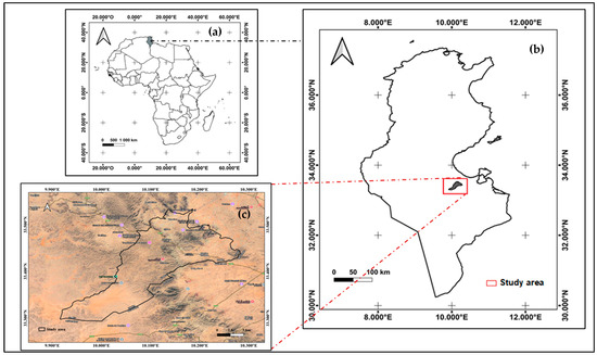
Figure 1.
Geographical location of the study region in Africa (a), southern Tunisia (b), and Google Earth base map (c).
2.2. SAVI
With technological advances and the emergence of free-to-use platforms such as the Climate Engine (available at www.climateengine.org, accessed on 22 March 2023), the task of mapping vegetation indices becomes easier. The Sentinel-2 SR (with a high spatial resolution of 10 m and an approximate 5-day revisiting cycle, already atmospherically corrected) dataset freely accessible from the European Space Agency was downloaded. The SAVI was calculated as monthly average during March 2018. Vegetation indices maps were produced based on the maximum photosynthetic period (March 2018) of the region of Toujane. This period aligns with the peak vegetation growth season in the study area. Additionally, 2018 as an exceptionally wet year (300 mm), serves as a suitable reference for assessing vegetation dynamics under favorable climatic conditions. Vegetation indices were calculated in QGIS (version 3.16.14), according to the following equation [9]:
where NIR is the near-infrared wavelengths, Red is the red wavelengths, and L is the soil adjustment factor (L = 0.5) [9]. NIR and Red are the reflectance of the infrared (Band 8: 842 nm) and red (Band4: 665 nm) bands of the Sentinel-2 SR sensor.
The final vegetation maps were then reclassified into three classes ‘high’, ‘medium’, and ‘low’ vegetation index classes using a K-means classification with the SAGA 7.2 tool. To predict SAVI changes, a regular grid with a mesh size of 0.089666° (≈10 km) was created. This grid was used to sample vegetation index classes, which were then saved as a csv file. The vegetation index classes are considered proxies for vegetation types to be modeled; the high SAVI comprises woods, olive trees, and crops; the medium SAVI includes shrublands and sparse olive trees; and the low SAVI gathers bare soil.
2.3. Data
Current (2020) and future (2021–2100) climatic data were downloaded from the Worldclim database (available at www.worldclim.org, accessed on 30 March 2023) using the two Shared Socioeconomic Pathways: SSP245 and SSP585. These SSPs belong to the General Circulation Model (GCM) from the Canadian Earth System Model version 5 (CanESM5). This model was selected based on its predictions that are near to the real climatic conditions of the study region. Nineteen bioclimatic variables were considered to analyze the current SAVI values and to run future model simulations. All of these variable’s layers were taken with a spatial resolution of 30 s (approximately 1 km2), expressed as minutes of a degree of longitude and latitude. Three topographic variables (elevation, aspect, and slope) were also considered. Elevation was calculated using the Digital Elevation Model (DEM) with a resolution of 30 m. Slope and aspect were calculated with the slope and aspects tools from the Spatial Analysis Tools of QGIS 3.16.14. In addition to the bioclimatic and topographic data, we downloaded some edaphic variables, like Bulk density, Carbon density, and Cation…, from the soil database (available at www.soilgrids.org, 250 m resolution, accessed on 22 March 2023). Finally, a set of 34 variables, including 19 bioclimatic, 3 topographic, and 12 soil variables, was obtained (Table 1). All data were transformed into ASCII files with the WGS84 datum using QGIS. The “Resampling” tool in QGIS was used to ensure that all variables had the same cell size (0.000269, 30 m × 30 m). The maximum entropy algorithm implemented in MaxEnt (3.4.4) was then run [13]. The full work is summarized in Figure 2.

Table 1.
General description of the studied bioclimatic, soil, and topographic variables.
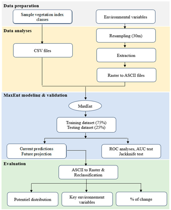
Figure 2.
Summary of the processing methodology and data analyses.
2.4. MaxEnt Modeling
MaxEnt is an open-source computer program that runs through the JAVA language. The occurrence points (samples) and environmental variables are entered as ASCII files to produce a probability map [14]. MaxEnt is executed with the following settings: maximum iterations = 500, convergence threshold of 10−5, and auto features, while other settings are maintained as default [15]. MaxEnt is used to simulate the potential current and future distribution of the SAVI and identify the environmental factors that impact this distribution [16]. MaxEnt employs the maximum entropy algorithm and land occurrence to predict the probability of land use [17]. For model calibration and assessment, 75% of the data is utilized for training while the remaining 25% is used to test the model’s predictive capabilities for SAVI distribution [18]. The automatic settings are applied for linear, quadratic, product, threshold, and hinge. The output of the Cloglog is utilized in the MaxEnt model to create a continuous map showing the predicted probability of presence ranging from 0 to 1. The test is conducted by excluding each variable systematically to evaluate the significance of environmental variables [18,19]. The MaxEnt model’s prediction accuracy is determined by the area under the curve (AUC) from the receiver operating characteristics (ROC) [20,21,22]. The AUC represents the probability that a randomly selected presence cell will have a higher predicted value than the selected absence one. Therefore, this metric evaluates the model’s ability to differentiate between area where the sample is present and area where it is not [13]. The accuracy of the model is confirmed through the use of AUC, which ranges from 0 to 1 [23]. The model’s predictive power increases with a greater numerical value. An AUC value of less than 0.5 indicates performance poorer than chance, whereas an AUC value of more than 0.75 indicates high performance, while a value of 1 signifies perfect discrimination [24,25]. The area under the receiving curve values between 0.5–0.7, 0.7–0.9, and 0.9–1.0 show low, moderate, and high predictions, respectively [26,27]. The jackknife procedure (regularized training gain) and percent variable contributions are applied to assess the relative influence of the considered variables [28].
All of the 34 variables are included in the model at the same time, following [29] observation that high collinearity poses a lesser issue for machine learning techniques compared to statistical models [27,30]. Furthermore, removing variables with high correlations does not improve MaxEnt models since the algorithm can handle redundant variables and reduce the effects of variable collinearity during model training [29]. Moreover, multicollinearity can lead to response curves that are not reliable because the impact of one factor is mixed up with its correlation to other factors, making it challenging to determine the actual effect of each predictor [31,32].
The MaxEnt outputs are in ASCII format, and QGIS is used to analyze and visualize the final forecasting maps [22]. According to the SAVI values, the SAVI forecasting map is classified into 4 sub-classes as follows: area with low class (0–0.25), moderate class (0.25–0.50), high class (0.50–0.75), and very high class (0.75–1). Classes represent, as said before, high-, medium-, and low-SAVI values. Four sub-classes will be obtained (low, moderate, high, and very high). Of course, the most important ones for the analysis are the very high sub-classes for each SAVI class; it was necessary to merge the presence probability maps for each SAVI sub-class to calculate the area values change for each vegetation sub-classes, scenario, and period to be analyzed.
3. Results
3.1. Model Performance
Based on the area under the receiving curve, the model showed good accuracy for both the high and low SAVI, with an AUC value ranging from 0.876 to 0.925 and from 0.76 to 0.885, respectively. In addition, a relatively robust sensitivity is obtained for the medium class (0.624–0.654) (Figure 3 and Figures S1–S6). It should be noted that high AUC shows a much greater level of accuracy in the model compared to random predictions.
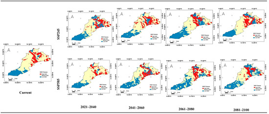
Figure 3.
SAVI classes for current and future situations of the study area under SSP245 and SSP585 scenarios from the CanESM5 model.
3.2. Influencing Variables
For high-SAVI distribution, the temperature seasonality (bio4), the temperature annual range (bio7), and the minimum temperature of the coldest month (bio6) are the strongest predictors. Precipitation of the warmest quarter (bio18), aspect, slope, bulk density, and coarse can also be considered important variables for the prediction. Concerning the medium SAVI, slope and some soil-related variables (nitrogen, clay content, bulk density, sand, and pH water) seem to be the key predictors. In contrast, for the low-SAVI, the results show that the precipitation of the driest month (bio14) is the strongest predictor (Figures S7 and S8).
3.3. Mapping Current and Future SAVI
The MaxEnt model results for the current and future SAVI under SSP245 and SSP585 scenarios are represented in Figure 3 and Table 2 using QGIS. The current high-SAVI class (woods, olive trees, and crops) is concentrated in the center of the study area and some parts of the eastern side and covers 1902.79 ha (Table 2). A slight increase in this class is noted under both SSP245 and SSP585 scenarios in 2030 and 2050. In 2070, this class is predicted to decrease from 3011.60 ha to 2442.72 ha, under SSP245, and from 2858.44 ha to 2492.09 ha under SSP585 (Table 2) and then will increase to reach, respectively, 3096.43 ha and 2624.41 ha in 2090.
Table 2.
SAVI area (ha) and respective percentages (%) during the different time periods and according to the SSP245 and SSP585 scenarios from the CanESM5 model. The most important sub-classes for the analysis (for each SAVI class) are indicated in bold.
The highest class of medium SAVI (shrublands and sparse olive trees) in the current situation occupies small locations in the north and south of the study area but it does not exceed 1316.63 ha. Based on SSP245 and SSP585, this class showed a clear fluctuation between years. Under SSP245, this class reaches its maximum in 2050 (4317.51 ha) and its minimum in 2090 (782.70 ha). Under SSP585, this class recorded a slight increase in area between 2030 (1484.35 ha) and 2090 (2145.83 ha).
Comparison between the current low-SAVI class (bare soil) and those of future situations for both SSP245 and SSP585 scenarios revealed similar trends (Figure 3, Table 2). The area of this class ranges from 3459.33 ha under SSP585 in 2070 to 4472.46 ha under SSP245 in 2090. The lowest area of this class (2943.00 ha) is recorded under SSP585 in 2090.
4. Discussion
Maximum entropy (MaxEnt) modeling has been proven to be an effective tool for future distribution of species/land uses/vegetation indices based on bioclimatic and soil variables [33]. The results indicate that this machine learning model provides a robust framework for predicting the distribution of the SAVI across the study area. With AUC values ranging from 0.876 to 0.925 for a high SAVI and 0.76 to 0.885 for a low SAVI, the model demonstrated good predictive accuracy, providing a strong analysis of the factors influencing SAVI distribution and its projected changes under future climate scenarios.
Through the contribution of each variable in the model and the jackknife test (Figures S7 and S8), this study reveals that climatic factors, particularly temperature-related parameters, are key drivers for the high-SAVI class. Air temperature seasonality (bio4), annual temperature range (bio7), and the minimum temperature of the coldest month (bio6) account for over 50% of the model’s prediction for a high-SAVI area. This result aligns with the existing literature, which suggests that temperature variability plays a crucial role in vegetation health and productivity, particularly in arid regions [34]. Rainfall also contributes to the model, with precipitation during the driest quarter (bio17). Changes in air temperature and rain are widely recognized as the primary factors affecting the survival, distribution, and growth of plants in arid and semi-arid regions [35,36]. Additionally, the terrain slope has secondary roles. Several studies emphasized the crucial role of topographical factors in enhancing the performance of the model [37]. For the medium-SAVI class, soil properties, including nitrogen content and bulk density, are identified as significant predictors, reflecting the influence of soil fertility and structure on vegetation growth. This finding is consistent with prior studies indicating that adding edaphic factors to the model greatly enhances the accuracy of projections [38,39]. For the low-SAVI class, precipitation patterns emerge as the dominant predictive factor. This highlights the sensitivity of low-SAVI vegetation types to water availability. As expected in regions disposed to drought or seasonal fluctuation in precipitation, these findings corroborate those of recent studies exploring vegetation responses to changing precipitation regimes [35]. Combining topographic and edaphic factors with bioclimatic variables, as demonstrated in this study, permits high accuracy of the models [5]. Taking into account that more precise predictors enhance the predictive capacity of any model [5,6,7,8,9,10,11,12,13,14,15,16,17,18,19,20,21,22,23,24,25,26,27,28,29,30,31,32,33,34,35,36,37,38,39,40], the variables used and their significance can be considered as best predictors in the MaxEnt model. Our finding suggested that all these variables have a strong contribution to SAVI prediction.
The spatial distribution of the current SAVI classes further emphasizes the heterogeneity in vegetation coverage across the study area. The high-SAVI class is currently concentrated in the central and eastern parts, while the medium-SAVI class occupies a smaller area in the northern and southern parts of the region. This distribution reflects the complex interactions between climatic conditions, topography, and soil properties. Both SSP245 and SSP585 scenarios predict a slight increase in the high-SAVI class during the near future (2030) in the northern region. Research investigating the impact of climate change on spontaneous vegetation indicates that plants are projected to migrate from their current habitats to higher elevations or more northern regions [5,41], but there will be a general decrease by the end of the century (2090). That is more pronounced under the SSP585 scenario, suggesting that future climate change may lead to a decline in vegetation productivity.
Under both future scenarios, the low-SAVI class is expected to increase, reflecting the shift to more arid conditions. The highest area for this class is predicted under SSP245 in 2090; however, the SSP585 scenario also indicates a significant increase in low-SAVI areas, particularly in 2070. This increase is probably due to the influence of some human activities that are not considered in modelization. In arid free-grazed rangelands, the pastoral plant tends to have lower covers/low SAVI compared with non-disturbed ones [42,43]. Vegetation is especially sensitive to both high disturbance and/or abiotic stress. This trend indicates a potential degradation of vegetation health, which could have effects on local ecosystems, particularly for grazing and agricultural activities dependent on vegetation cover.
5. Conclusions
This study applied MaxEnt modeling and the CanESM5 climate projections to evaluate the impacts of climate change on the SAVI in Toujane’s arid rangelands. Temperature and precipitation are the most influential factors. Under the high-emission scenario of SSP585, significant SAVI reductions are projected by 2080, hence showing the vulnerability of such ecosystems. These results highlight the need for adaptive management strategies, such as mentioning specific strategies, to improve the resilience of natural rangelands.
Supplementary Materials
The following supporting information can be downloaded at: https://www.mdpi.com/article/10.3390/cli13030059/s1, Figure S1: Average omission rate and predicted area of high SAVI as a function of the cumulative threshold for current (a) and futures (b: 2021–2040; c: 2041–2060; d: 2061–2080; e: 2081–2100) scenarios under SSP245. The respective receiver operating characteristic (ROC) curves are f, g, h, i, j.; Figure S2: Average omission rate and predicted area of medium SAVI as a function of the cumulative threshold for current (a) and future (b: 2021–2040; c: 2041–2060; d: 2061–2080; e: 2081–2100) scenarios under SSP245. The respective receiver operating characteristic (ROC) curves are f, g, h, i, j.; Figure S3: Average omission rate and predicted area of low SAVI as a function of the cumulative threshold for current (a) and future (b: 2021–2040; c: 2041–2060; d: 2061–2080; e: 2081–2100) scenarios under SSP245. The respective receiver operating characteristic (ROC) curves are f, g, h, i, j.; Figure S4: Average omission rate and predicted area of high SAVI as a function of the cumulative threshold for current (a) and future (b: 2021–2040; c: 2041–2060; d: 2061–2080; e: 2081–2100) scenarios under SSP585. The respective receiver operating characteristic (ROC) curves are f, g, h, i, j.; Figure S5: Average omission rate and predicted area of medium SAVI as a function of the cumulative threshold for current (a) and future (b: 2021–2040; c: 2041–2060; d: 2061–2080; e: 2081–2100) scenarios under SSP585. The respective receiver operating characteristic (ROC) curves are f, g, h, i, j.; Figure S6: Average omission rate and predicted area of low SAVI as a function of the cumulative threshold for current (a) and future (b: 2021–2040; c: 2041–2060; d: 2061–2080; e: 2081–2100) scenarios under SSP585. The respective receiver operating characteristic (ROC) curves are f, g, h, i, j.; Figure S7: Current and future jackknife for the studied variables under SSP245; Figure S8: Current and future jackknife for the studied variables under SSP585.
Author Contributions
Conceptualization, J.M., A.T. and M.T.; methodology, J.M. and A.T.; software, F.C.; validation, M.T.; formal analysis, J.M. and A.T.; investigation, M.T.; writing—original draft preparation, J.M.; writing—review and editing, J.M.; supervision, M.T.; project administration, M.T. and A.R.; funding acquisition, M.T. and A.R. All authors have read and agreed to the published version of the manuscript.
Funding
This work was supported by the own budget of the Arid Regions Institute of Médenine (Tunisia) and the PASTINNOVA project: «Innovative models for sustainable future of Mediterranean pastoral systems» financed by PRIMA foundation-section 1 (Grant Agreement number 2113, 2022–2025).
Data Availability Statement
Data are available through a reasonable request from the corresponding author.
Acknowledgments
We are grateful to the anonymous reviewers for their important contributions to this document.
Conflicts of Interest
The authors declare no conflicts of interest.
References
- Mikhaylov, A.; Moiseev, N.; Aleshin, K.; Burkhardt, T. Global climate change and greenhouse effect. Entrep. Sustain. Issues 2020, 7, 2897. [Google Scholar] [CrossRef]
- Trenberth, K.E. Climate change caused by human activities is happening and it already has major consequences. J. Energy Nat. Resour. Law 2018, 36, 463–481. [Google Scholar] [CrossRef]
- Vani, V.; Mandla, V.R. Comparative study of NDVI and SAVI vegetation indices in Anantapur district semi-arid areas. Int. J. Civ. Eng. Technol. 2017, 8, 559–566. [Google Scholar]
- Skendžić, S.; Zovko, M.; Lešić, V.; Pajač Živković, I.; Lemić, D. Detection and Evaluation of Environmental Stress in Winter Wheat Using Remote and Proximal Sensing Methods and Vegetation Indices. Diversity 2023, 15, 481. [Google Scholar] [CrossRef]
- Dülgeroğlu, C.; Aksoy, A. Assessing impacts of climate change on Campanula yaltirikii H. Duman (Campanulaceae), a critically endangered endemic species in Turkey. Turk. J. Bot. 2019, 43, 243–252. [Google Scholar] [CrossRef]
- Lemenkova, P.; Debeir, O. Computing Vegetation Indices from the Satellite Images Using GRASS GIS Scripts for Monitoring Mangrove Forests in the Coastal Landscapes of Niger Delta, Nigeria. J. Mar. Sci. Eng. 2023, 11, 871. [Google Scholar] [CrossRef]
- Harris, N.R.; Louhaichi, M.; Johnson, D.E. Laboratory Manual for Landscape Ecology, Spatial Analysis of Landscape Data, Lab 9. In Landscape Ecology and Analysis; Department of Rangeland Resources, Oregon State University: Corvallis, OR, USA, 2004. [Google Scholar]
- Almutairi, B.; El Battay, A.; Belaid, M.A.; Musa, N. Comparative Study of SAVI and NDVI Vegetation Indices in Sulaibiya Area (Kuwait) Using Worldview Satellite Imagery. Int. J. Geosci. Geomat. 2013, 1, 50–53. [Google Scholar]
- Huete, A.R. A soil-adjusted vegetation index (SAVI). Remote Sens. Environ. 1988, 25, 295–309. [Google Scholar] [CrossRef]
- Ahmad, F. Spectral vegetation indices performance evaluated for Cholistan Desert. J. Geogr. Reg. Plann. 2012, 5, 165–172. [Google Scholar]
- Zhao, S.; Pereira, P.; Wu, X.; Zhou, J.; Cao, J.; Zhang, W. Global karst vegetation regime and its response to climate change and human activities. Ecol. Indic. 2020, 113, 106208. [Google Scholar] [CrossRef]
- Ben Salem, F. Study of the Phytocenosis Dynamics in the Alfa Steppe (Stipa tenacissima L.) Under the Effects of Drought and Human Activities: Case of the Monts of Matmata. Ph.D. Thesis, University of Carthage, Carthage, Tunisia, 2012; 197p. [Google Scholar]
- Phillips, S.J.; Anderson, R.P.; Dudík, M.; Schapire, R.E.; Blair, M.E. Opening the black box: An open-source release of MaxEnt. Ecography 2017, 40, 887–893. [Google Scholar] [CrossRef]
- Anderson, R.P.; Lew, D.; Peterson, A.T. Evaluating predictive models of species distributions. Criteria for selecting optimal models. Ecol. Model. 2003, 162, 211–232. [Google Scholar] [CrossRef]
- Phillips, S.J.; Dudik, M.; Schapire, R.E. A maximum entropy approach to species distribution modeling. In Proceedings of the Twenty-First International Conference on Machine Learning, Banff, AB, Canada, 4–8 July 2004; pp. 655–662. [Google Scholar]
- Yan, H.; Feng, L.; Zhao, Y.; Feng, L.; Wu, D.; Zhu, C. Prediction of the spatial distribution of Alternanthera philoxeroides in China based on ArcGIS and MaxEnt. Glob. Ecol. Conserv. 2020, 21, e00856. [Google Scholar] [CrossRef]
- Abolmaali, S.M.R.; Tarkesh, M.; Bashari, H. MaxEnt modeling for predicting suitable habitats and identifying the effects of climate change on a threatened species, Daphne mucronata, in central Iran. Ecol. Inform. 2018, 43, 116–123. [Google Scholar] [CrossRef]
- Duan, X.; Li, J.; Wu, S. MaxEnt Modeling to Estimate the Impact of Climate Factors on Distribution of Pinus densiflora. Forests 2022, 13, 402. [Google Scholar] [CrossRef]
- Yang, X.Q.; Kushwaha, S.P.S.; Saran, S.; Xu, J.; Roy, P.S. MaxEnt modeling for predicting the potential distribution of medicinal plant, Justicia adhatoda L. in Lesser Himalayan foothills. Ecol. Eng. 2013, 51, 83–87. [Google Scholar] [CrossRef]
- Wang, Y.S.; Xie, B.Y.; Wan, F.H.; Xiao, Q.M.; Dai, L.Y. The Potential Geographic Distribution of Radopholus similis in China. Agric. Sci. China 2007, 6, 1444–1449. [Google Scholar] [CrossRef]
- Coban, O.; Örücü, Ö.K.; Arslan, E. MaxEnt Modeling for Predicting the Current and Future Potential Geographical Distribution of Quercus libani Olivier. Sustainability 2020, 12, 2671. [Google Scholar] [CrossRef]
- Zhou, Y.; Zhang, Z.; Zhu, B.; Cheng, X.; Yang, L.; Gao, M.; Kong, R. MaxEnt Modeling Based on CMIP6 Models to Project Potential Suitable Zones for Cunninghamia lanceolata in China. Forests 2021, 12, 752. [Google Scholar] [CrossRef]
- Fielding, A.H.; Bell, J.F. A review of methods for the assessment of prediction errors in conservation presence/absence models. Environ. Conserv. 1997, 24, 38–49. [Google Scholar] [CrossRef]
- Swets, J.A. Measuring the accuracy of diagnostic systems. Science 1988, 240, 1285–1293. [Google Scholar] [CrossRef]
- Peavey, L. Predicting Pelagic Habitat with Presence-Only Data Using Maximum Entropy for Olive Ridley Sea Turtles in the Eastern Tropical Pacific. Master’s Thesis, Duke University, Durham, NC, USA, May 2010. [Google Scholar]
- Pearce, J.; Ferrier, S. Evaluating the predictive performance of habitat models developed using logistic regression. Ecol. Model. 2000, 133, 225–245. [Google Scholar] [CrossRef]
- Elith, J.; Graham, C.H. Do they? How do they? Why do they differ? On finding reasons for differing performances of species distribution models. Ecography 2009, 32, 66–77. [Google Scholar] [CrossRef]
- Yost, A.C.; Petersen, S.L.; Gregg, M.; Miller, R. Predictive modeling and mapping sage grouse (Centrocercus urophasianus) nesting habitat using Maximum Entropy and a long-term dataset from Southern Oregon. Ecol. Inform. 2008, 3, 375–386. [Google Scholar] [CrossRef]
- Feng, X.; Park, D.S.; Liang, Y.; Pandey, R.; Papeş, M. Collinearity in ecological niche modeling: Confusions and challenges. Ecol. Evol. 2019, 9, 10365–10376. [Google Scholar] [CrossRef] [PubMed]
- Hu, W.; Wang, Y.S.; Zhang, D.; Yu, W.; Chen, G.; Xie, T.; Liu, Z.; Ma, Z.; Du, J.; Chao, B. Mapping the potential of mangrove forest restoration based on species distribution models: A case study in China. Sci. Total Environ. 2020, 748, 142321. [Google Scholar] [CrossRef] [PubMed]
- De Marco, P.J.; Nóbrega, C.C. Evaluating collinearity effects on species distribution models: An approach based on virtual species simulation. PLoS ONE 2018, 13, e0202403. [Google Scholar] [CrossRef] [PubMed]
- Luna, S.; Peña-Peniche, A.; Mendoza-Alfaro, R. Species distribution model accuracy is strongly influenced by the choice of calibration area. Biodivers. Inform. 2024, 10, 18. [Google Scholar] [CrossRef]
- Capera-Aragones, P.; Tyson, R.C.; Foxall, E. The maximum entropy principle to predict forager spatial distributions: An alternate perspective for movement ecology. Theor. Ecol. 2023, 16, 21–34. [Google Scholar] [CrossRef]
- Schilling, J.; Freier, K.P.; Hertig, E.; Scheffran, J. Climate change, vulnerability and adaptation in North Africa with focus on Morocco. Agric. Ecosyst. Environ. 2012, 156, 12–26. [Google Scholar] [CrossRef]
- Zhong, W.; Xue, J.; Li, X.; Xu, H.; Ouyang, J. A Holocene climatic record denoted by geochemical indicators from Barkol Lake in the northeastern Xinjiang, NW China. Geochem. Int. 2010, 48, 792–800. [Google Scholar] [CrossRef]
- Nielsen, U.N.; Ball, B.A. Impacts of altered precipitation regimes on soil communities and biogeochemistry in arid and semi-arid ecosystems. Glob. Change Biol. 2015, 21, 1407–1421. [Google Scholar] [CrossRef]
- Lassueur, T.; Joost, S.; Randin, C.F. Very high-resolution digital elevation models: Do they improve models of plant species distribution? Ecol. Model. 2006, 198, 139–153. [Google Scholar] [CrossRef]
- Buri, A.; Cianfrani, C.; Pinto-Figueroa, E.; Yashiro, E.; Spangenberg, J.E.; Adatte, T.; Verrecchia, E.; Guisan, A.; Pradervand, J.N. Soil factors improve predictions of plant species distribution in a mountain environment. Prog. Phys. Geogr. 2017, 41, 703–722. [Google Scholar] [CrossRef]
- Dubuis, A.; Rossier, L.; Pottier, J.; Pellissier, L.; Vittoz, P.; Guisan, A. Predicting current and future spatial community patterns of plant functional traits. Ecography 2013, 36, 1158–1168. [Google Scholar] [CrossRef]
- Pradervand, J.N.; Dubuis, A.; Pellissier, L.; Guisan, A.; Randin, C. Very high-resolution environmental predictors in species distribution models: Moving beyond topography? Prog. Phys. Geogr. 2014, 38, 79–96. [Google Scholar] [CrossRef]
- Walther, G.R.; Post, E.; Convey, P.; Menzel, A.; Parmesan, C.; Beebee, T.J.; Fromentin, J.M.; Guldberg, O.H.; Bairlein, F. Ecological responses to recent climate change. Nature 2002, 416, 389–395. [Google Scholar] [CrossRef] [PubMed]
- Ouled Belgacem, A.; Ben Salem, F.; Gamoun, M.; Chibani, R.; Louhaichi, M. Revival of traditional best practices for rangeland restoration under climate change in the dry areas: A case study from Southern Tunisia. Int. J. Clim. Change Strateg. Manag. 2019, 11, 643–659. [Google Scholar] [CrossRef]
- Msadek, J.; Tlili, A.; Moumni, M.; Louhaichi, M.; Tarhouni, M. Impact of Grazing Regimes, Landscape Aspect, and Elevation on Plant Life Form Types in Managed Arid Montane Rangelands. Rangel. Ecol. Manag. 2022, 83, 10–19. [Google Scholar] [CrossRef]
Disclaimer/Publisher’s Note: The statements, opinions and data contained in all publications are solely those of the individual author(s) and contributor(s) and not of MDPI and/or the editor(s). MDPI and/or the editor(s) disclaim responsibility for any injury to people or property resulting from any ideas, methods, instructions or products referred to in the content. |
© 2025 by the authors. Licensee MDPI, Basel, Switzerland. This article is an open access article distributed under the terms and conditions of the Creative Commons Attribution (CC BY) license (https://creativecommons.org/licenses/by/4.0/).