Feedback Trends with ECS from Energy Rates: Feedback Doubling and the Vital Need for Solar Geoengineering

Simple Summary

Global warming (GW) occurs when we add greenhouse gasses (GHGs) like CO₂ and darken the Earth with black roads and roofs. This is called “forcing” in climatology. Warming due to forcing is increased by nature’s feedback problems like snow and ice melting which makes the planet hotter as we lose reflectivity. But as the planet loses reflectivity and warms, more snow and ice melt, and this is called a feedback loop. Most of the feedback and feedback loop problems are due to atmospheric water vapor, which is increasing as the planet becomes hotter. This is because warmer air holds more water vapor. More water vapor in the atmosphere is a problem because water vapor is a strong GHG. This study estimates that water vapor GHG increase is 83% of the total feedback problem. In short, global warming is the sum of forcing and feedback problems. Most people are concerned about CO₂ forcing problems from emissions (from cars, power plants, etc.). However, this study estimates that GW due to feedback in 2024 has become larger than forcing with about 54% due to feedback and 46% due to forcing. Although forcing causes feedback, it is unlikely that if we could remove all the forcing (CO₂, etc.) that feedback would also fully reverse since we are over the 50% point. This adds to our global warming risks. This study estimates feedback trends over time with simple graphs which helps us better understand our global warming root causes. Calculations for these are based on simple data manipulation on how much faster global warming occurs, compared to energy consumption. This is shown to provide feedback estimates. Results show that, in 2024, forcing, what man does, like adding CO₂, is now less of a problem than what nature’s feedback warming is doing, like adding water vapor and the snow and ice melting. Because GW due to feedback is larger now than forcing, this study highly recommends that we should try and mitigate feedback as well. There are two methods to mitigate global warming: reducing manmade GHGs (a secondary warming source) and/or using solar geoengineering (SG). SG is 62% more efficient than CO₂ reduction as it uses methods to reduce the Sun’s energy (the primary warming source) absorbed by the Earth, to help cool it. For example, we could brighten our streets and roofs to reflect the sunlight away, to reduce the amount of heat absorbed. However, we will need stronger solar geoengineering methods, which likely will include ways to reflect sunlight away in the stratosphere and/or in outer space. GHG current mitigation methods are likely far too slow to keep up with the rate of aggressive feedback increases and CO₂ lingers in the atmosphere for 100’s of years. Furthermore, GHG reduction efforts have been disappointing, with many obstacles other than emission problems, like wildfires, and lack of worldwide unification with the U.S. again pulling out of the Paris Agreement. Therefore, given the current circumstances including feasibility, it is unfortunate, but we should not expect that we can mitigate GW using only GHG reduction methods according to a risk assessment provided here. There are currently no strong SG efforts, which can take years to develop and implement. There are no guidelines in the Paris Agreement to stop even the opposite problem of the critical worldwide abuse of dark roads, roofs, cars, and buildings, a form of negative SG. Candidates for SG besides urbanization include the Arctic and Antarctic to help cool the planet. In this paper, the method called annual SG, which can help stop yearly GW increases to stabilize temperature increase problems, is urgently recommended while GHG reduction methods can improve. SG implementation will take years to develop and urgently requires the help of organizations like NASA, Space X, and the Canadian, Chinese, and European space agencies.

Abstract

This paper provides climate feedback trends, quantifies the feedback-doubling (FD) period, considers urbanization influences, and provides related equilibrium climate sensitivity (ECS) estimates using data from 1880 to 2024. Data modeling is accomplished by focusing on statistically significant stable normalized correlated rates (NCRs, i.e., normalized related slopes). Estimates indicate that the global warming NCR is increasing by a factor of 1.65 to 2.33 times faster than the energy consumption NCR, from 1975 to 2024. The reason is feedback amplification. This is supported by the fact that the NCR for forcing and energy consumption shows approximate equivalency in the period studied. Results provide feedback yearly trend estimates at the 95% confidence level that key results will fall within the IPCC AR6 likely range. The projected 2017–2024 feedback amplification estimates, using the EC approach, range from 2.0 to 2.16, respectively. A feedback amplification of 2.0 (approximately equal to −2.74 Wm⁻² K⁻¹) doubles the forcing, indicating that in 2024, more than half of global warming (53.7%) is likely due to feedback. Relative to the feedback-doubling (FD) threshold (i.e., the point where feedback exceeds forcing), the FD overage is 3.7% in 2024. This is the amount of feedback exceeding the FD threshold found to have a surprisingly aggressive 3.1% to 3.9% estimated overage growth rate per decade. We now ask, shouldn’t we try to mitigate feedback as well as GHG forcing, and if forcing could be removed, how would global warming fully “self-mitigate”? Additionally, CO₂ yearly increases are complex, with poor reduction progress. Therefore, this study’s risk assessment urgently recommends supplementary “mild” annual solar geoengineering as a minimum requirement, to reduce the dominant aggressive feedback. SG reduces the primary solar warming source creating 62% higher mitigation efficiency than CDR. Urgency is enhanced since solar geoengineering must be timely and can take years to develop. This study also estimates that 75% to 90.5% (83% average) of the feedback problem is due to water vapor feedback (WVF). High WVF also plagues many cities needing local SG. Trend analysis indicates that by 2047, the earliest we may reach 10 billion people, feedback amplification could reach a value of 2.4 to 2.8. Furthermore, by 2082, the year estimated for 2× CO₂, at the current rate, feedback amplification could range from 2.88 to 3.71. This yields an ECS range from 2.4 °C to 3.07 °C, in reasonable agreement with the reported estimated range in AR6. An overview of recent urbanization forcing attribution indicates the ECS value may be lower by 10.7% if this forcing is considered. For numerous reasons, the lack of albedo urbanization Earth brightening requirements in the Paris Agreement, is unsettling and urgently needed. In addition, a model assesses effective forced feedback (EFF) temperature characteristics of up to 1.9 °C, providing interesting feedback insights that may relate to high GW land and pipeline temperature estimates. Lastly in addition to urbanization, solar geoengineering in the Arctic and Antarctic is advised. Worldwide efforts in GHG mitigation, with no significant work in SG, appears highly misdirected.

1. Introduction

In this paper, the anthropogenic effects of global warming are studied through normalized correlated rate (NCR) trend analysis due mainly to energy consumption (EC). CO₂ and population changes are also assessed. The goal of this paper is to use statistically significant highly stable NCRs and modeling to help provide feedback amplification yearly trend estimates (Figure 1a) at the 95% confidence level relative to the IPCC AR6 likely values (see Section 3.1.1). These are important in assessing the ECS value (Section 3.2.3) and GW root causes (Figure 1b), along with what is defined as feedback doubling (FD) and its strength. This is aided by the fact that data appear to be fairly linear in the 1975 to 2022 period and somewhat nonlinear from 2022 to 2024, key areas of interest in this study. Data are supplemented with small adjusted GW estimates from 1880 to 1974. All data used in this study are provided in Appendix A. Linear and exponential feedback trend projections for various periods (1880 to 2082) are provided (see figures in Section 3.1).

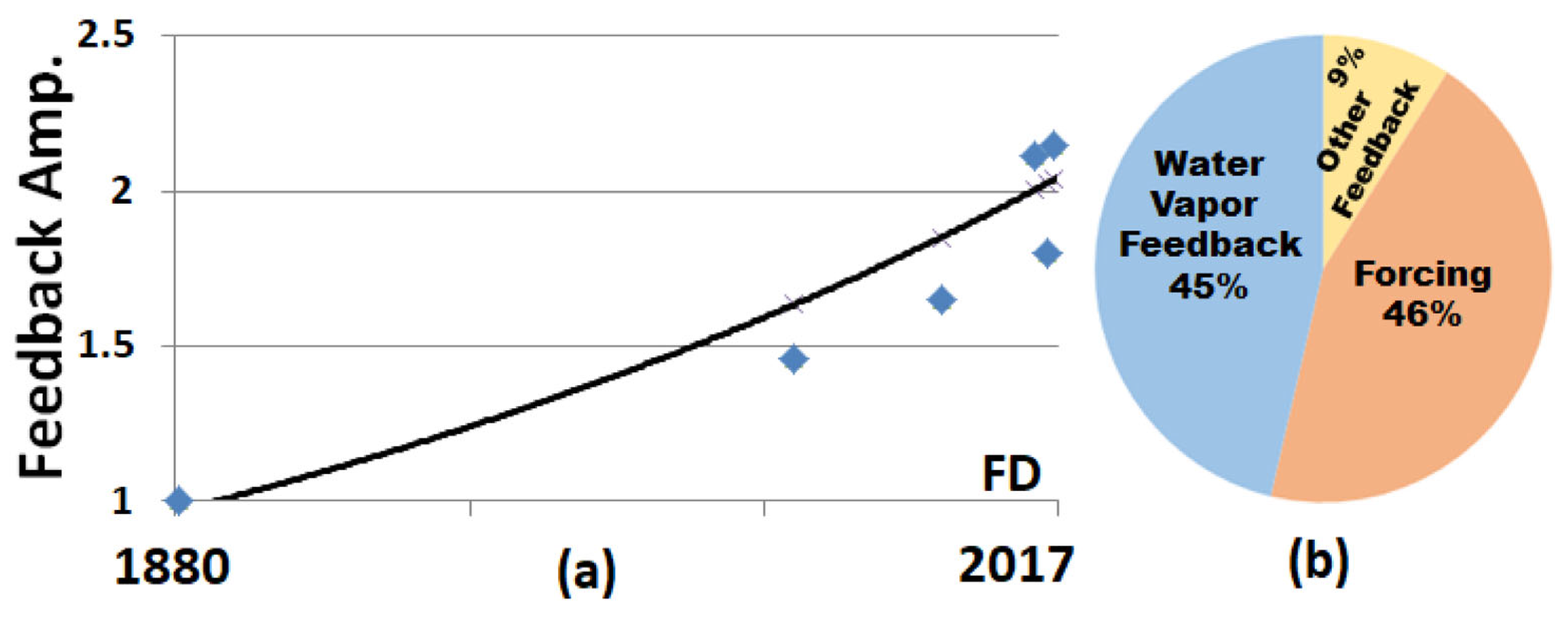
This study also illustrates the practical use of the feedback amplification (A_{Feedback Amp}) metric, a simple unitless number compared to the complex common feedback values. For example, GW equates to forcing × A_{Feedback Amp} (Equation (11)), and the percent of GW due to feedback is simply (A_{Feedback Amp} − 1)/A_{Feedback Amp} (see Appendix B.1 and Equation (13)). 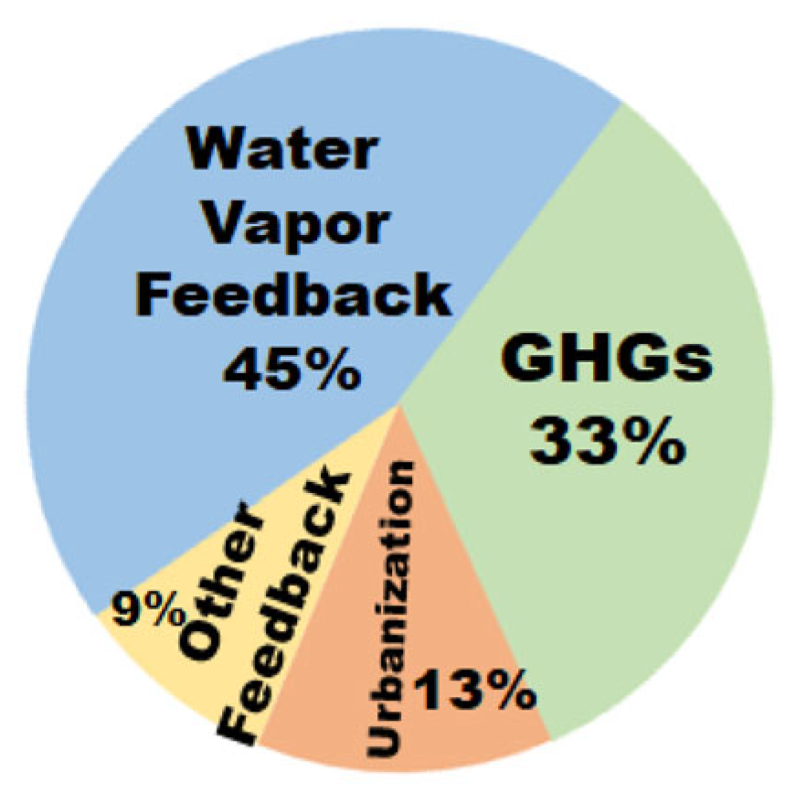For example, in 2024 a value of A_{Feedback Amp} = 2.14 indicates that about 54% of GW is due to feedback (see Figure 1b) with 83% of the feedback problem due to water vapor. Additionally, SG reverse forcing estimates need to incorporate the background climate feedback effect, which is simplified using the A_{Feedback Amp} value (Equation (21)). Therefore, this work provides the reader with perhaps the only study of its kind that offers yearly trend estimates as shown in Figure 1a using the practical feedback amplification metric, helping to better assess and interpret the temporal feedback problem (see Section 3.1 for graphical details). Furthermore, this is likely the first study to define the FD point and strongly recommend the need for significant solar geoengineering mitigation.

The feedback amplification value, A_{Feedback Amp.}, is estimated by the NCR ratio for GW to EC (see Equation (10)) with its statistically significant highly stable correlated rates (Section 3.1). It is important to note that correlations do not prove causation. However, they help assess obvious relationships and trends. Results prove insightful. Using the NCR method, this study finds that the energy consumption and the forcing NCRs show approximate equivalency in the period of this study. This important result allows for these basic graphical NCR feedback amplification estimates (see Section 2.1, Equation (10) and its example, in Section 3.2). This is further supported by a derivation (see Section 2.1) and data in this period that demonstrates their approximate equivalency. Additionally, feedback amplification converted to feedback values compares well with reported AR6 estimates, including this study’s ECS assessments, lending support to this equivalency. We can see that NCR graphical methods with up-to-date data provide statistically significant stable estimates over recent time periods with post-industrial adjustments (1880–1974). This provides greatly simplified modeling methods for estimating feedback trends, leading to ECS values that compare well to IPCC AR6 likely estimates and those of highly complex helpful studies [1].

NCR feedback amplification assessment indicates a large increase from 2022 to 2024, which appears to correlate to a jump in stratospheric water vapor that started in 2022 (see Figures in Section 4). However, other researchers [2] suggest that this may not be the case. An analysis is provided in Section 4.

This study estimates using the EC approach that the feedback strength became higher than the forcing strength after 2017 (Equation (10)), with an average of 83% of the feedback problem due to water vapor (Figure 1b, see Section 3.2.1). This is denoted as an FD threshold (Section 3.1.2) when A_{Feedback Amp} > 2 (Figure 1a). Here we question, if feedback is now greater than forcing, shouldn’t we try and mitigate feedback as well as GHG forcing, and would global warming fully reverse if forcing could be removed [3,4]? Also, assessed is CO₂ reduction progress over important time periods, one observes complex yearly atmospheric CO₂ increases (this is detailed in Appendix F and Section 3.6). That is, CO₂ atmospheric reductions are complex, mainly due to emissions, are often confounded by wildfires, deforestation, volcanic eruptions, and wars, and the fact that some countries (including the U.S.), are not participating in the Paris Agreement, making it increasingly problematic to achieve IPCC RCP goals, as detailed in Section 3.6. It is also difficult for the IPCC to categorize CO₂ completely from the many complex sources, but these are mostly accounted for in the EC method (Section 3.6). Therefore, given the many obstacles in obtaining a significant CO₂ reduction and considering that the FD overage level is increasing at a rate or about 3.1% to 3.9% per decade (see Section 3.3), this study’s risk assessment strongly requires for at least additional emergency “mild” annual solar geoengineering [5] reverse-forcing mitigation methods to reduce feedback and GW trends. This is urgent due to the length of time required to develop solar geoengineering, which can take 10–20 years to develop (see Section 4.3) and must be done in a timely manner. Currently, the feedback amplification and forcing increase rates are in similar ranges, increasing the GW’s rate higher than its components.

Other authors have proposed that FD by water vapor may have occurred as early as 2013 [6,7]. In Section 3.1.1, this study’s trend estimates find that FD occurred in 2017 and water vapor FD occurred in 2024 or later. The amount above the 50% FD value is defined here as the FD overage level (Figure 1a) that may be difficult to model. It is not suggested that the FD threshold is a tipping point (see graphical abstract), as many climatologists [8] interpret a tipping point as a “tipping over” irreversible point. However, it is viewed here as a threshold where feedback exceeds forcing.

A risk assessment and discussion in Section 4.3 indicate the extraordinary high risks of not carrying out SG ASAP. In Section 3.6, global warming mitigation issues using population control and trying to achieve significant CO₂ reductions are also assessed.

In Section 3.5, the feedback amplification rate of change with a temperature derivative using a graphical method is analyzed. The results provide EFF characteristic temperatures up to 1.9 °C. While it is unconventional to attribute EFF temperatures, several insights related to land and pipeline temperatures are made.

In Section 3.4, urbanization GW influences are detailed and supported up to the 13% GW level. In Section 3.5, the supportive work of Zhao et al. [9] is noted, who reported that UHIs in wet climates are about 3.3 °C higher than comparable UHIs in dry climates. Feinberg [10] reported that the WVF of UHIs in wet climates, based on Zhao et al.’s [9] study, found values over a factor of two higher than the background WVF climate. We note that about 67% of the population lives in humid mostly urban climates [11,12] where negative SG (dark roads, roofs, etc.) is unrestricted.

Results of this study show that there are numerous serious solar geoengineering requirements, and realistically, GHG reduction methods are not a strong enough option to offset GW surprisingly aggressive feedback in a timely manner, as GHGs linger in the atmosphere for 100’s of years and have numerous complex sources (Section 3.6). SG based on the primary warming source, the Sun, is 62% more efficient (Appendix B.3, [13,14]) compared to CDR, which is a secondary warming source. Possible candidates for SG, discussed in Section 4.2, are the Arctic and Antarctic areas that help cool the planet. If these areas could be saved, global warming increases may be limited, and tipping elements can be avoided, which reside in the cryosphere [15]. We need help from NASA, Space X, and the Canadian, Chinese, and European space agencies to help develop the technologies required to even implement mild Annual SG [5] for Earth brightening, SAI, and space sunshading. SG technologies are needed now but will take years to develop.

Overview of Topics

Table 1. Topics covered and their sections.

Overview of Topics	Section
Introduction	Section 1
Overview of topics	Overview of Topics
Methods and data	Section 2
Derivation illustrating how energy consumption and the forcing NCRs show equivalency, helping to provide feedback estimates	Section 2.1
Trend assumptions and limitations	Section 2.2
Results	Section 3
Normalized correlated rate assessments for feedback amplification (AFeedback)	Section 3.1
Feedback trend analysis and statistical significance estimates	Section 3.1.1
Feedback doubling likely occurred in 2017	Section 3.1.2
Feedback amplification in the CO2 doubling year	Section 3.1.2
Amplified-feedback-correlated-rate comparisons to AR6 estimates	Section 3.2
Global water vapor feedback amplification factors and percentage estimates	Section 3.2.1
The CO2 doubling year	Section 3.2.2
ECS value and feedback estimate for the doubling year 2082	Section 3.2.3
Feedback amplification estimates for different scenarios including RCP projections	Section 3.3
The effect of urbanization attribution on forcing and the ECS value	Section 3.4
AFeedback Amp characteristic temperature rate of change and EFF temperatures and urbanization issues	Section 3.5
Interpretation of the EFF temperature	Section 3.5.1
Interpretation of the UHI WVF and hydro-hotspot issues	Section 3.5.2
Aerosols and urban WVF	Section 3.5.3
Global warming mitigation issues using population control and trying to achieve IPCC RCP CO2 reduction goals	Section 3.6
Discussion: Recent trend analysis for CO2, feedback, and global warming due to high water vapor trends	Section 4
Observations of water vapor increase correlated with the global warming increase	Section 4.1
Solar geoengineering for the Arctic and Antarctic to limit global warming	Section 4.2
Mild solar geoengineering mitigation requirements: Pushback confusion and risk assessment	Section 4.3
Summary	Section 5
Data used in graphs and analysis	Appendix A
Feedback percent of GW-energy rates of change with forcing and SG mitigation efficiency	Appendix B
Feedback estimates using radiation forcing	Appendix C
GW-feedback-forcing NCR and feedback amplification derivation	Appendix D
Comparison between NCR for EC and CO2 forcing and feedback estimates	Appendix E
Recent nonlinear global warming trends and CO2 reduction problems	Appendix F

provides an overview of the topics covered and how this paper is organized.

2. Methods and Data

Many authors link energy consumption, driven by population growth, to climate forcing. This is primarily due to GHG emissions [16,17,18,19,20,21] with contributions from black carbon smoke and soot solar heating effects [22,23,24], anthropogenic heat release [25], and the UHI effect [25,26]. Numerous studies also show the benefits of renewable energies in helping reduce climate forcing [18,19,20,21]. Additionally, new hydrogen fuel efforts will help reduce CO₂ emissions, especially in aviation [27]. Section 2.1 provides the basic equations and methods used in this study. There approximate equivalency between energy consumption and forcing is shown in the period of this study, along with data to support this finding.

To access EC, we can use the total global energy production and consumption increase for coal, oil, natural gas, and other sources as calculated by Ritchie and Roser [28] up to the year 2021; this is shown in Figure 2 by the top line (data provided in Appendix A). More recent data by the Energy Institute [29] confirm that these observed trends continued through 2024.

Interestingly, the slope of the energy curve (Figure 2) is about 2184 TWh/year from 1974 to 2021. This is estimated from the ordinary regression analysis. EC has reduced slightly in the last 10 years to about 2153 TWh/year (Appendix A).

In Figure 2, the global warming (GW) trend (land and ocean) is shown by the bottom line [30] (see Appendix A). These data are smoothed as provided by NASA [30]. An ordinary t-test on energy consumption and unsmoothed global warming data finds a p-value of 1 × 10⁻³⁰, showing a strong likely relationship between the two datasets, with a Pearson correlation of 93.4% for unsmoothed GW data and 98.88% for smoothed GW data (see Appendix A). However, it appears that GW is increasing at a faster rate than EC.

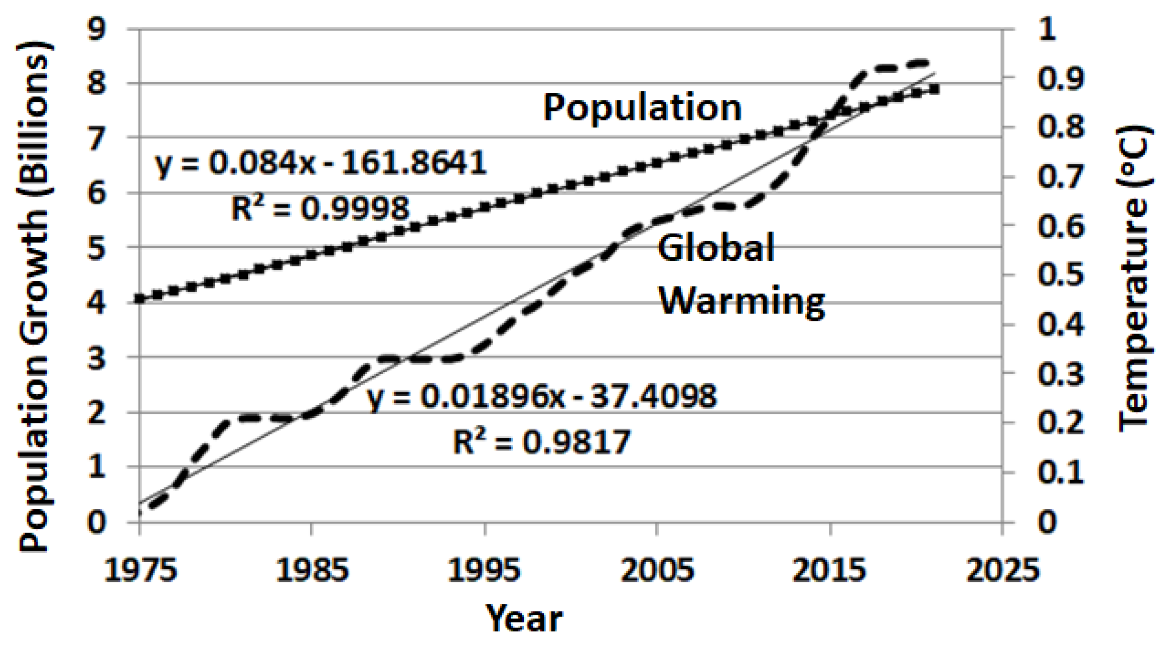
Similarly, in Figure 3, the population growth rate [31] (see Appendix A) is shown (top line), along with (land and ocean) global warming (bottom line for smoothed data). A t-test on population and global warming data (Figure 3) finds a p-value of 1 × 10⁻³⁸, showing a strong likely relationship between the two datasets, with a Pearson correlation of 98.98% for smoothed GW data and 94.4% for unsmoothed data. However, it appears that global warming is increasing at a faster rate than population growth.

A t-test on the anticipated correlation between CO₂ ppm increase and global warming data (in Appendix A) finds a p-value of 4.4 × 10⁻⁵⁶, showing a strong relationship between the two datasets, with a Pearson correlation of 94.5% for unsmoothed data. A t-test on the anticipated correlation between CO₂ ppm increase and energy consumption data (in Appendix A) finds a p-value of 1.2 × 10⁻²⁹, showing a strong relationship between the two datasets, with a Pearson correlation of 99.7% from 1977 to 2019.

We anticipate that more information and modeling are needed to understand the relationship between CO₂ and GW increases, as detailed in Section 3. One notes that methane also contributes to GW, and is assessed as part of the EC totals.

We can see from Figure 3’s equation, for example, the average population increase per year from the relatively short-term trend is

$$\begin{gathered} {\displaystyle Y(2021)-Y(2020)=\left(0.084 \times 2021-161.93\right)-\left(0.084 \times 2020-161.93\right) \\ =7.834BP-7.75BP=0.084BP} \end{gathered}$$

(1)

The increase is about 0.084 billion people (BP) from 2020 to 2021. This is a population growth rate (PGR) of

$$\mathrm{PGR}=1-7.834/7.75=1\% \mathrm{per} \mathrm{year}$$

(2)

This agrees fairly accurately with most estimates for 2021 [31]. The population growth rate has varied from about 2.1% down to the recent estimate of about 0.9% [31]. Using the graphical equation for population growth in Figure 3, when we insert the year 2047, this trend equation indicates that we may reach 10 billion people (BP) by 2047. This is a little sooner than the Worldometer estimate of 2060, which considers an eventual slower population growth rate.

2.1. Derivation Illustrating How Energy Consumption and the Forcing NCRs Show Equivalency, Helping to Provide Feedback Estimates

In this proof, we start by assuming that a change in forcing is due to a change in energy consumption, such that (using the chain rule)

$$\mathsf{\Delta }F={\displaystyle \frac{\mathsf{\partial }F}{\mathsf{\partial }EC}}\mathsf{\Delta }EC$$

(3)

Here, ΔF represents forcing change, and ΔEC represents energy consumption change. To simplify, let ‘a’ equate to the partial derivative in Equation (3), such that $a={\displaystyle \frac{\mathsf{\partial }F}{\mathsf{\partial }EC}}$. Then, dividing through Equation (3) by a time period Δt to introduce a rate of change yields

$$\left({\displaystyle \frac{\mathsf{\Delta }\mathrm{F}}{\mathsf{\Delta }t}}\right)=a\left({\displaystyle \frac{\mathsf{\Delta }EC}{\mathsf{\Delta }t}}\right)$$

(4)

Here, Δt represents the time period of interest. Figure 2 indicates that the energy consumption slope is fairly constant from 1975 to 2022, such that ΔE/Δt ≈ dEC/dt. We can introduce the feedback λ equation and utilize Equation (4) as follows:

$$\mathrm{Feedback}=\lambda =-{\displaystyle \frac{\mathsf{\Delta }\mathrm{F}}{\mathsf{\Delta }\mathrm{T}}}=-\left({\displaystyle \frac{\mathsf{\Delta }\mathrm{F}}{\mathsf{\Delta }t}}\right)/\left({\displaystyle \frac{\mathsf{\Delta }{T}_S}{\mathsf{\Delta }t}}\right)\cong -a\left({\displaystyle \frac{\mathsf{\Delta }EC}{\mathsf{\Delta }t}}\right)/\left({\displaystyle \frac{\mathsf{\Delta }{T}_S}{\mathsf{\Delta }t}}\right)$$

(5)

To assess feedback amplification requires unitless NCRs of change. This involves dividing each time series value by the maximum series value (see the Results section for details and normalized figures). Using unitless NCRs per unit of time, we find the inverse feedback-to-feedback amplification relationship is

$${\mathrm{A}}_{\mathrm{Feedback} \mathrm{Amp}.}={\left(1/\lambda \right)}_{\mathrm{NCR}}\cong a_{NCR}{{\left({\displaystyle \frac{\mathsf{\Delta }{T}_S}{\mathsf{\Delta }t}}\right)}_{NCR}/\left({\displaystyle \frac{\mathsf{\Delta }EC}{\mathsf{\Delta }t}}\right)}_{NCR}$$

(6)

Here, A_{Feedback Amp.} is the feedback amplification value (≥1). Note that since we are using unitless series values for ΔT_S and ΔEC, now a_NCR in Equation (6) will also be unitless. We will find below that a_NCR≈1. As an example of using Equation (6) with a_NCR ≈ 1, feedback amplification values are tabulated in the tables in Section 3. For example, from the figures in Section 3, we have

$${\left({\displaystyle \frac{\mathsf{\Delta }{T}_S}{\mathsf{\Delta }t}}\right)}_{NCR}={\left({\displaystyle \frac{\mathsf{\Delta }GW}{\mathsf{\Delta }t}}\right)}_{NCR}=0.0204 {\mathrm{yr}}^{-1}$$

$$\mathrm{and} {\left({\displaystyle \frac{\mathsf{\Delta }EC}{\mathsf{\Delta }t}}\right)}_{NCR}=0.0124 {\mathrm{yr}}^{-1}$$

$$\mathrm{and} \mathrm{yields} {\mathrm{A}}_{\mathrm{Feedback} \mathrm{Amp}.}\cong {{\left({\displaystyle \frac{\mathsf{\Delta }{T}_S}{\mathsf{\Delta }t}}\right)}_{NCR}/\left({\displaystyle \frac{\mathsf{\Delta }EC}{\mathsf{\Delta }t}}\right)}_{NCR}=1.65$$

This is one of the values listed in the tables in Section 3.1.

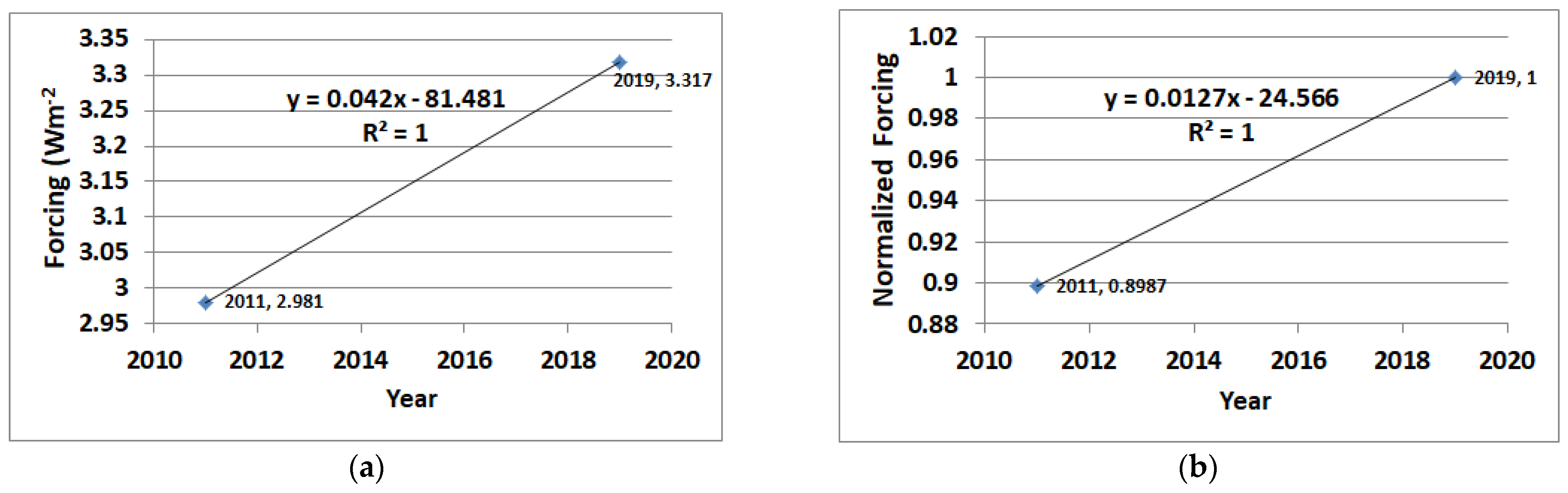
To show that a_NCR ≈ 1, we can estimate the normalized forcing and energy rates to find its actual value. Figure 4 plots the IPCC forcing estimates for 2011 and 2019 from Chapter 7 of WGI in AR6 (see Table 7.5 in Ref. [32]). We can plot these data points along with their normalized forcing.

Then, from Equation (4), we can compare Figure 4b for the NCR of forcing to the results in Section 3 (second figure), with a slope of 0.0124 Yr⁻¹ for the NCR of energy consumption, which helps us find the value of a_NCR, where

$$a_{NCR}\cong {{\left({\displaystyle \frac{\mathsf{\Delta }\mathrm{F}}{\mathsf{\Delta }t}}\right)}_{NCR}/\left({\displaystyle \frac{\mathsf{\Delta }EC}{\mathsf{\Delta }t}}\right)}_{NCR}=0.0127 {\mathrm{yr}}^{-1}/0.0124 {\mathrm{yr}}^{-1}=1.024$$

(7)

The results indicate that we can take a_NCR as

$$a_{NCR}\cong 1.0$$

(8)

Energy dynamics may change due to a reduction in fossil fuel use [33]. However, for this study, in the estimated period of about 1975 to 2022, the current assessment indicates that the NCR of energy consumption is approximately equal to the NCR of forcing, i.e.,

$${\left({\displaystyle \frac{\mathsf{\Delta }EC}{\mathsf{\Delta }t}}\right)}_{NCR}\cong {\left({\displaystyle \frac{\mathsf{\Delta }F}{\mathsf{\Delta }t}}\right)}_{NCR}$$

(9)

Figure 4’s data points at first appear to provide low confidence. However, this equivalency is further supported in this period, in the Results section, with comparisons to IPCC AR6 likely values, as shown in Section 3.1.1, Section 3.2, and Section 3.3 (ECS values). This increases statistical confidence in Equation (9), as assessed in Section 3.1.1. EC modeling may have the advantage of easily incorporating more CO₂ sources than IPCC ERF assessments (see Section 3.6) due to the ratio in Equation (10).

We now can estimate from Equations (6) and (9) the EC model for feedback amplification used in this study, as

$$\boxed{{\mathrm{A}}_{\mathrm{Feedback} \mathrm{Amp}.}\cong {{\left({\displaystyle \frac{\mathsf{\Delta }{T}_S}{\mathsf{\Delta }t}}\right)}_{NCR}/\left({\displaystyle \frac{\mathsf{\Delta }EC}{\mathsf{\Delta }t}}\right)}_{NCR}}$$

(10)

This illustrates that the energy consumption NCR will likely provide reasonable feedback estimates. The results using Equation (10) are provided in Section 3.1 and Section 3.2 for feedback and feedback amplification estimates.

To further clarify the feedback amplification factor, A_{Feedback Amp} is ≥1 and amplifies the forcing, such that

$${\left(\mathsf{\Delta }{T}_S\right)}_{Power}={\left(\mathsf{\Delta }GW\right)}_{Power}={\mathrm{A}}_{\mathrm{Feedback} \mathrm{Amp}.}\times \mathsf{\Delta }F$$

(11)

This is more formally derived in Appendix D.

From Equations (6) and (11), we have

$$\boxed{\mathrm{Feedback}=\lambda =-{\displaystyle \frac{\mathsf{\Delta }F}{\mathsf{\Delta }{\mathrm{T}}_{\mathrm{S}}}}={\displaystyle \frac{{\left(\mathsf{\Delta }GW\right)}_{Power}/{\mathrm{A}}_{\mathrm{Feedback} \mathrm{Amp}.}}{\mathsf{\Delta }{\mathrm{T}}_{\mathrm{S}}}}}$$

(12)

This is the key equation for converting feedback amplification to feedback (and vice versa). Also, see Equation (17) for water vapor feedback conversions. Several estimates are provided in Section 3.1, Section 3.2, Section 3.3, using Equation (12), and the results compared well to AR6 feedback and ECS values.

In Appendix B.1, it is shown that the percent of GW due to feedback can be estimated as

$$\boxed{\%\mathrm{of}\mathrm{GW} \mathrm{due} \mathrm{to} \mathrm{Feedback}={\displaystyle \frac{{\mathrm{A}}_{\mathrm{Feedback} \mathrm{Amp}.}-1}{{\mathrm{A}}_{\mathrm{Feedback} \mathrm{Amp}.}}}, for{\mathrm{A}}_{\mathrm{Feedback} \mathrm{Amp}.}\ge 1}$$

(13)

See the table in Section 3.3 for current and future estimates including RCP scenarios. In that table, reverse forcing SG estimates are also provided, with an example of how to calculate SG requirements that are greatly simplified using the A_{Feedback Amp} factor (see Equation (21) and Ref. [8]). SG reverse forcing requirements are thus another important use of the feedback amplification metric.

It is interesting to note that a similar approach to Equation (3) could have been taken, using a CO₂ instead of an EC approach. Some estimates are provided in Appendix E for the interested reader to illustrate that similar findings to those in this paper can be obtained using a CO₂ NCR forcing method.

2.2. Trend Assumptions and Limitations

While there are a large number of data points in Figure 2 and Figure 3, Figure 4’s data are small in size. To supplement this lack of data in Figure 4, comparisons to IPCC AR6 results can be included. This will increase engineering confidence. As well, we can rely on IPCC modeling to increase statistical confidence in Section 3.1.1. Therefore, the results in this study are estimated to fall within the IPCC likely range with 95% statistical confidence (Section 3.1.1). Note that the climate is complex and modeling is not an exact science.

In Section 3.6, it is pointed out that there are many sources of atmospheric CO₂, which can confound forcing estimates. The EC approach helps in this regard, as it is more correlated with anthropogenic CO₂ forcing and other sources (Section 3.6) and how modeling divides this out so feedback can be estimated.

The climate system is constantly changing. Recent GW variations in 2022–2024 show the difficulty of providing trend estimates compared to the earlier linear periods up to 2022. As well, this study focuses on temperature, a key thermodynamic driver. However, this can be limiting as the climate is more complex. Nevertheless, NCR analysis helps reduce variations and is viewed in this study as showing graphical stability, allowing for reasonable statistical estimates.

3. Results

The key drivers of global warming dynamics are considered to be feedback, energy consumption, CO₂, and population changes. Methane is also an important contributor to GW but is not reviewed in this study as it is not part of the ECS analysis. Although an assessment of methane NCR would be insightful, it would not add substantially to this paper’s findings as results are provided using the EC method. However, methane is assessed as part of the EC totals.

In this paper, the analysis uses NCR assessment, so data are normalized to a maximum value of 1, which also provides unitless values per year for comparative purposes. Normalized data are provided in Appendix A at their maximum values in 2021–2022. This is done to find feedback trend estimates per Section 2.1.

Results using this method are first shown for the normalized global warming data and population growth (see Appendix A) in Figure 5. For example, the data for population growth has a maximum value of 7.88 billion people in Figure 3. Then all data are divided by this maximum value. This yields for example, in 2005, from the graph, that the population growth is at about 80% of the maximum 7.88 billion people (BP) value that occurred in 2022, which puts it at about 6.3 BP in 2005. Also, in Figure 5 is global warming normalized to its maximum 2022 value of 0.9 °C (Appendix A).

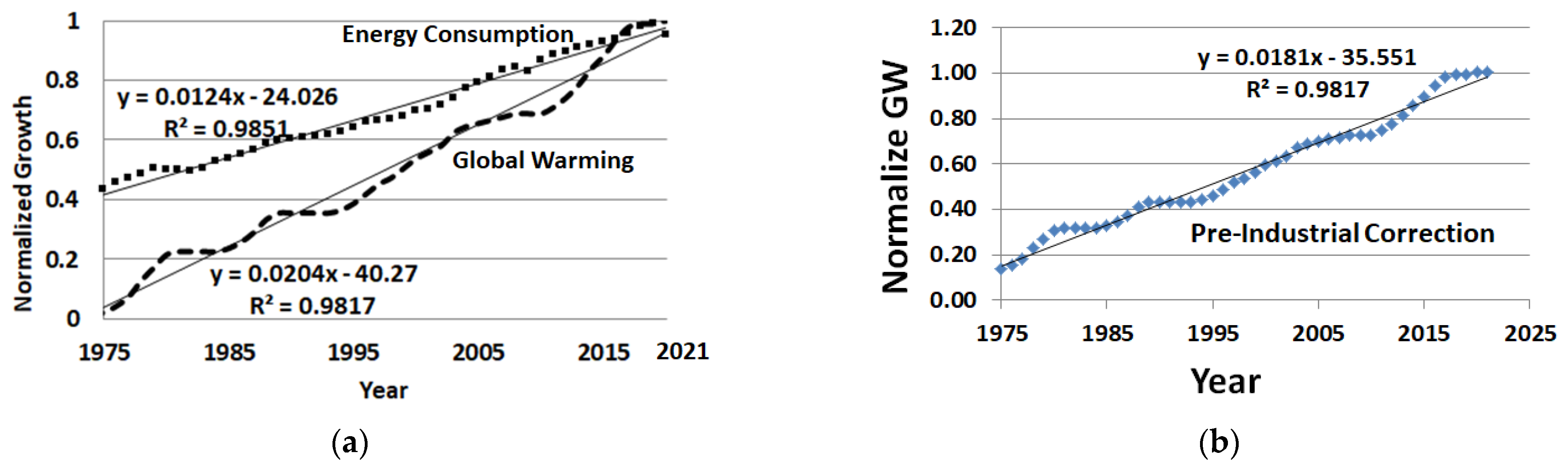
In Figure 6, similar results are shown for energy consumption normalized to its maximum value of 176,431 TWh in 2021, along with normalized global warming.

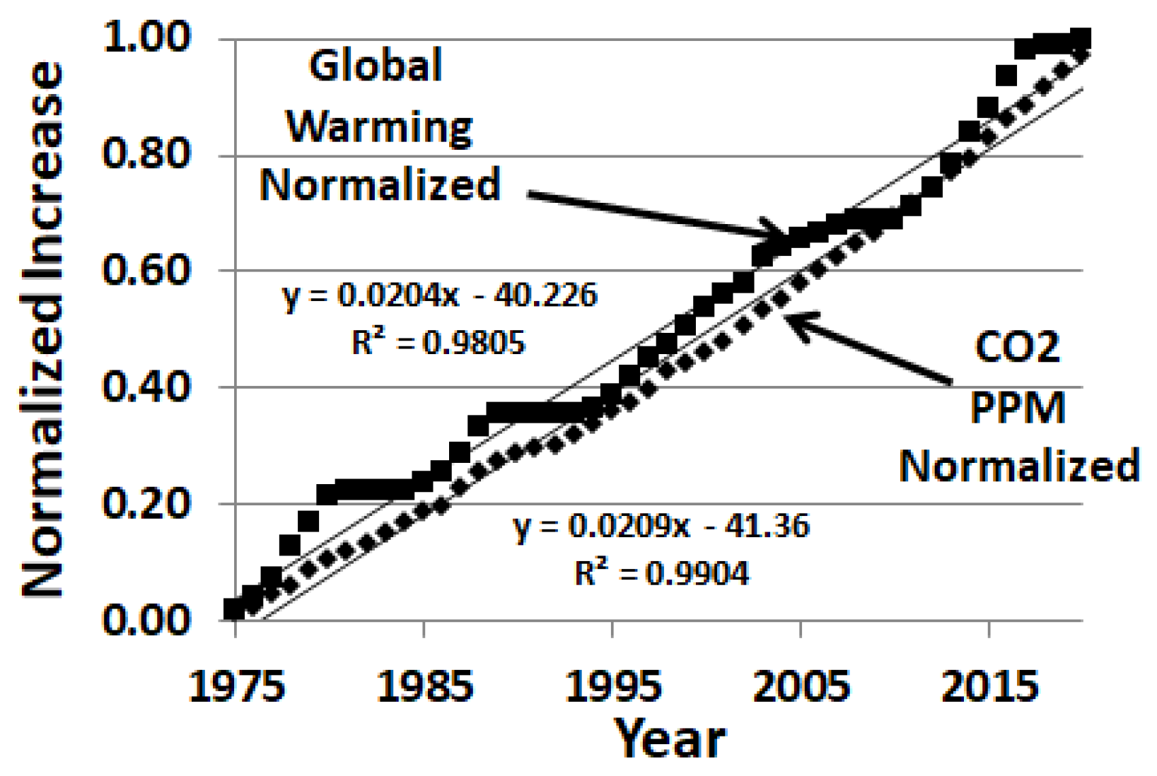
Figure 7 displays the increases for CO₂ data normalized to 418.6 ppm in 2022, along with global warming normalized data.

3.1. Normalized Correlated Rate Assessments for Feedback Amplification (A_{Feedback Amp.})

Using the normalized unitless data methods reduces complexity so that slopes displayed in the graph can be compared. Assessing slopes also reduces time lag issues when the gradients are fairly constant over time, providing high statistical confidence (see Section 3.1.1). The following normalized correlated rates (NCRs) are found for the period of 1975–2021: 0.0204/year for global warming, 0.0209/year for CO₂ increase, 0.0107/year for population growth, and 0.0124/year for energy consumption. Data are highly correlated in Figure 5 and Figure 6, for smoothed data with statistically significant correlations with R ≥ 0.99, and R ≥ 0.965 for unsmoothed data in Appendix A. The NCR assessments indicate that global warming and CO₂ (Figure 7) are increasing by a factor of 1.9 times faster than population growth and 1.65 times faster than energy consumption. However, when this is adjusted to the earlier period (1880–2021), the global warming normalized slope is 0.0181/year (see Figure 6b). To obtain an early post-industrial estimate from 1880–1974, a 0.15 °C approximate rise [30] was added to each data point, yielding an increase in 2021 of 1.05 °C (Appendix A). This changes the normalization factor, which changes the slope (see Figure 6b). These early post-industrial NCR assessments are lower and indicate that global warming is increasing by a factor of 1.62 times faster than population growth and 1.46 times faster than energy consumption for the years 1900–2021, with the average year in this interval of 1960.

There are strong correlations between GW and population growth and between energy consumption and global warming. However, since different countries consume energy at different rates, population growth is likely not the best metric to use in assessing global warming correlations. Therefore, in this study, global warming feedback assessments are based on comparisons with energy consumption’s NCRs.

The amount of amplification is denoted by the factor A_{Feedback Amp.} (see Table 2). These amplification A_{Feedback Amp.} values relative to the NCRs between global warming and energy consumption are shown in Table 2, with the average year taken similar to 1960 (for 1900 to 2022). Here, using the simple ratio method in Equation (10) for feedback amplification estimates, we can realize that the likely reason that the GW NCRs are 1.46 and 1.65 times faster than the energy consumption normalized slope from 1900–2021 and 1975–2021, respectively, as shown in Table 2, is due to a correlated feedback amplification effect, as shown in Section 2.1 by Equation (10).

Section 3.2 provides comparative feedback amplification to feedback estimates. In Appendix C, an overview of this feedback and radiative forcing estimates help to illustrate that A_{Feedback Amp.} values compared well to feedback estimates. The amplification in the recent period of 1977 to 2022 is displayed in Table 2.

Table 2. Feedback amplification (A_{Feedback Amp.}) estimates (see also Table in Section 3.3).

Average Year	AFeedback Amp. Estimates	Net Feedback * Wm−2 K−1	Average ΔTobs (°C)	Period (Years)
1975	1.46	−3.71	0.25	1900–2022
2000	1.65	−3.3	0.44	1975–2022
2016	2.11
2018	1.80
2019	2.15 (Figure 8)	−2.55	0.95	2019
2025	2.37 [34]	NA	NA	2025
	Projected estimate to 10 BP
2047	2.42

* Does not include the Planck estimate of 3.22 Wm⁻² K⁻¹.

Table 2. Feedback amplification (A_{Feedback Amp.}) estimates (see also Table in Section 3.3).

Average Year	AFeedback Amp. Estimates	Net Feedback * Wm−2 K−1	Average ΔTobs (°C)	Period (Years)
1975	1.46	−3.71	0.25	1900–2022
2000	1.65	−3.3	0.44	1975–2022
2016	2.11
2018	1.80
2019	2.15 (Figure 8)	−2.55	0.95	2019
2025	2.37 [34]	NA	NA	2025
	Projected estimate to 10 BP
2047	2.42

* Does not include the Planck estimate of 3.22 Wm⁻² K⁻¹.

Figure 8. Feedback amplification trend analysis (Table 2) assessed using NCR methods: (a) 1975–2019 data–linear fit (b) 2000–2019 data plus 2025 Hansen et al. [34] point–linear fit (c) 1870–2082 Exponential fit with added unity and 2× CO₂ point from linear fit (d) 1940–2082 Exponential fit with added unity, plus Hansen et al. [34] point and 2× CO₂ estimate from linear fit.

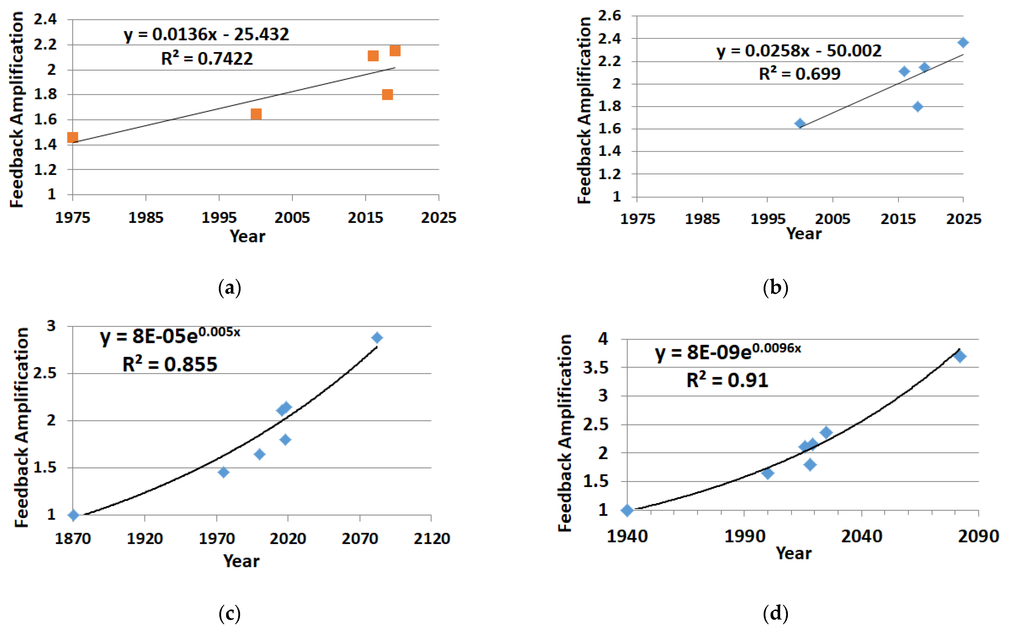
Figure 8. Feedback amplification trend analysis (Table 2) assessed using NCR methods: (a) 1975–2019 data–linear fit (b) 2000–2019 data plus 2025 Hansen et al. [34] point–linear fit (c) 1870–2082 Exponential fit with added unity and 2× CO₂ point from linear fit (d) 1940–2082 Exponential fit with added unity, plus Hansen et al. [34] point and 2× CO₂ estimate from linear fit.

3.1.1. Feedback Trend Analysis and Statistical Significance Estimates

Figure 8a displays the NCR analysis results in Table 2 for feedback amplification trends from 1975 to 2019 using the EC NCR approach. Figure 8b displays the additional data point due to Hansen et al.’s [34] pipeline estimate of global warming increase affecting feedback (see recent trends in Section 4). This increase in feedback in Figure 8b may be due to the surge in water vapor, displayed in the figures of Section 4 in the period from 2022 to 2024, and is discussed in Section 3.2.1 and Section 4. Note in Figure 8a,b a linear fit was used and it is easier to note the amplification trend is increasing at about 0.136 per decade which compared well to the exponential fit used in Figure 8c,d.

Figure 8c exponential fit has an added unity amplification data point that was estimated to occur in 1870 when fitting the upper data points. Similarly, Figure 8d displays an exponential fit, but with the added Hansen et al. [34] pipeline estimate. Figure 8d fit was problematic as the unity point occurred in 1940 to fit the upper data points. In both Figure 8c,d estimates, 2× CO₂ points were added based on the linear extrapolation in Figure 8a,b to the year 2082 (see Section 3.2.2), respectively. These are needed in Section 3.2.3 for ECS estimates.

In Table 2, the standard error in the Y-values is about ±1.5% with 95% statistical confidence due to the large number of data points over 49 years for GW and EC NCR data with a p-value of 1 × 10⁻³⁷. However, the standard error for X-values is problematic due to the few data points in Figure 8a,b. A slope analysis for Figure 8a,b finds p-values of 0.06 and 0.078. A p-value greater than 0.05 indicates a lack of statistical significance. However, using Figure 8a,b projections to the year 2082, the estimated time for 2× CO₂ to occur (detailed in Section 3.2.2) results in values of 2.88 and 3.714, respectively. Using these values, the ECS estimated range proves to match likely estimates in IPCC AR6. Then, the projection to the year 2082 proves to be reasonably accurate, increasing confidence in the slopes found in Figure 8a,b. When these points are added to increase the data points in these figures, the p-values for Figure 8a,b slopes drop to 0.0019 and 0.005. These are well below the 0.05 p-value threshold, indicating that slopes are statistically significant at the 95% confidence level in producing key results that fall within the IPCC AR6 likely range using the EC method (Equation (10)).

Figure 8c,d p-values are 0.00289 and 0.00084, respectively. These are well below the 0.05 level indicating reasonable statistical significance. However, we note that Figure 8d is confounded since the unity value in the likely fit for upper data points falls around 1940 instead of closer to 1880. However, these exponential fits are helpful as often authors estimate that feedback likely increases exponentially in time. As well, climate amplification is often viewed to have started around 1950 in most graphical estimates [30] so the 1940 value in Figure 8d may be somewhat acceptable.

Note that we now have reasonable statistical confidence to equate feedback amplification values to the percent of global warming (using Equation (13)). For example, the projected value in 2024 using Figure 8a’s equation yields an A_{Feedback Amp.} of 2.16, which equates to 53.7% of GW being due to feedback per Equation (13). These estimates are provided in the table in Section 3.3 and include different RCP scenarios and reverse forcing assessments as well. It is illustrated in Equation (21) how to use the A_{Feedback Amp.} value for SG estimates.

3.1.2. Feedback Doubling Likely Occurred in 2017

Trend analysis in the linear fitted line indicates that feedback amplification is increasing by a factor of 0.136 (Figure 8a) to 0.161 (Figure 8b) per decade, as determined using the EC NCR approach to estimate forcing. The R² fit is greater than 74%, with a correlation factor R above 86%, as shown in Figure 8, and higher regression R² values are found in the exponential fits in Figure 8. The trend analysis equations in Figure 8a,c for the earlier time period are used to estimate the FD year. This indicates that since 2016 to 2017, the feedback strength has been slightly more than the forcing strength (A_FeedbackAmp. > 2). This indicates a key FD area of concern since feedback has become larger than forcing. Also, we can question if we should be trying to mitigate feedback as well as GHG forcing, and if we could take away all the forcing, would the climate be fully mitigated? Such activity has been described [3,4]. Doubling of the forcing due to water vapor feedback was described as early as 2013 by Dessler et al. [6]; as the paper stated, “tropospheric moistening more than doubles the direct warming from carbon dioxide.” Additionally, Gordon et al. in 2013 [7] concluded (for 2002–2009 data), “water vapor changes in the climate system, which, acting alone, would double the magnitude of any warming forced by increasing greenhouse gas concentrations.” However, this study’s 2017 estimate for FD can only attribute 75% to 91% (Section 3.2.1) to water vapor feedback. Estimates in this study indicate that this water vapor portion of FD may have occurred as early as 2024, but likely not before then.

Feedback estimates are considered to be dominated by water vapor feedback, as exemplified in Section 3.2.1 (75% to 90%, averaging 83%). In comparison, the author found a value of feedback amplification of 2.15 as early as 2019 [13] (Table 2) using other modeling methods, suggesting this threshold may have been passed earlier. If there was no feedback amplification (i.e., A_{Feedback Amp.} = 1), we would anticipate that NCR slopes should be about the same in Figure 6a. The A_{Feedback Amp.} in Table 2, displayed in Figure 8, indicates that feedback increased by about 43% from 1975 (1.46) to 2024 (2.07).

NCR assessments also find that the energy consumption rate is slightly higher than the population growth rate, by a factor of 1.159 in the 1977 to 2022 time period. We note that most energy consumption occurs within cities, and this is overviewed on the GW urbanization influence in Section 3.4.

3.2. Amplified-Feedback-Correlated-Rate Comparisons to AR6 Estimates

From Figure 8a, results indicate an amplification estimate of about 2.04 occurred in 2019. In that year, a 0.95 °C increase was observed, which using the Stephan–Boltzmann relation, equates to a GW power of 5.2 Wm⁻¹. Then, using Equation (12), the 2019 feedback estimate is

$$\begin{array}{cc}\mathrm{Feedback}=\lambda & =-{\displaystyle \frac{\mathsf{\Delta }F}{\mathsf{\Delta }{\mathrm{T}}_{\mathrm{S}}}}=-{\displaystyle \frac{{\left(\mathsf{\Delta }GW\right)}_{Power}/{\mathrm{A}}_{\mathrm{Feedback} \mathrm{Amp}.}}{\mathsf{\Delta }{\mathrm{T}}_{\mathrm{S}}}}\hfill \\ & =-{\displaystyle \frac{{\left(5.2\right)}_{Power}/2.04}{0.95}}=-2.7 {\mathrm{Wm}}^{-2}{\mathrm{K}}^{-1}\end{array}$$

(14)

Then, the total forcing estimate in 2019 is

$$\mathsf{\Delta }\mathrm{F}=-\lambda \mathsf{\Delta }{T}_S=-(-2.7 {\mathrm{Wm}}^{-2}{\mathrm{K}}^{-1})(0.95 K)=2.6 {\mathrm{Wm}}^{-2}$$

(15)

This value is close to Table 7.8 in AR6 Ch. 7 [32] (1750–2019), estimating a total forcing of 2.72 Wm⁻² (with an AR6 range of 1.96 to 3.48 Wm⁻² [32]).

From Equation (12), we can estimate that portion of feedback due to CO₂, yielding

$$\begin{array}{ll}{\mathrm{Feedback}}_{{\mathrm{CO}}_2}& ={\lambda }_{{CO}_2}=-{\displaystyle \frac{\mathsf{\Delta }{F}_{{\mathrm{CO}}_2}}{\mathsf{\Delta }{\mathrm{T}}_{\mathrm{S}}}}=-{\displaystyle \frac{{\left(\mathsf{\Delta }GW\right)}_{Power\_{CO}_2}/{\mathrm{A}}_{\mathrm{Feedback} \mathrm{Amp}.}}{\mathsf{\Delta }{\mathrm{T}}_{\mathrm{S}}}}\hfill \\ & =-{\displaystyle \frac{{\left(5.2\right)}_{Power}0.794/2.04}{0.95}}=-2.1 {\mathrm{Wm}}^{-2}{\mathrm{K}}^{-1}\hfill \end{array}$$

(16)

Note the 0.794 factor comes from AR6 Ch. 7 Table 7.8, where CO₂ forcing is 2.16 Wm⁻² and the total forcing is 2.72 Wm⁻², their ratio yields the CO₂ portion of 0.794. As a check, the CO₂ forcing would be about $2.1 {\mathrm{Wm}}^{-2}{\mathrm{K}}^{-1}\times 0.97 \mathrm{K}=2.06 {\mathrm{Wm}}^{-2}$, which reasonably compares to the AR6 value of 2.16 Wm⁻² in AR6 Chapter 7 Table 7.8.

3.2.1. Global Water Vapor Feedback Amplification Factors and Percentage Estimates

It is interesting to estimate the water vapor feedback amplification portion of feedback. Gordon et al. [7] estimated a water vapor feedback of 2.4 Wm⁻² K⁻¹. For a 1 K global temperature rise, which equates to about 5.1 Wm⁻² (Equation (14)), this yields a positive feedback amplification value (Equation (11)) of

$$\boxed{A_{Amp\_Water\_Vapor}={\displaystyle \frac{5.1 {\mathrm{Wm}}^{-2}}{5.1 {\mathrm{Wm}}^{-2}-2.4 {\mathrm{Wm}}^{-2}{\mathrm{K}}^{-1}\times 1.0 \mathrm{K}}}=1.81}$$

(17)

Note that in the denominator, instead of the general forcing term 2.4 Wm⁻² K⁻¹ × 1.0 K, we want to use the feedback power quantity, which is shown in the denominator (i.e., GW = feedback power + forcing). Therefore, we subtract the forcing from the GW power to obtain the feedback power.

As a second estimate, Liu et al. [35] estimated a water vapor feedback of 1.6 Wm⁻² K⁻¹ at a global temperature near 14 °C from 2004 to 2016. For a 1 K global temperature rise, using Liu et al.’s [35] estimate in Equation (C-1), this would yield an amplification of 1.5. We note a similar estimate: Dessler [6], for the earlier period of 2000–2010, yielded 1.2 Wm⁻² K⁻¹. This increasing trend can be observed in the figures in Section 4 (9 and 10).

In 2019, a value of 2.0 for feedback amplification was used (Equation (14)). Then we noted the values indicate that feedback amplification is dominated by water vapor feedback, at about 75% to 90.5% (i.e., 1.5 or 1.81 divided by 2.0).

3.2.2. The CO₂ Doubling Year

We can take 2× CO₂ = 570 ppm, where 1× CO₂ = 285 ppm. It is important to estimate the year in which CO₂ will double to approximate an ECS value from the current trend analysis. The CO₂ increase is fitted using a linear estimate, shown in Figure 9 over recent years.

From the linear fitted data in Figure 9, if the trend were to continue, we anticipate the doubling year for 570 ppm to occur in 2082 using the linear fit equation. With this estimate, the feedback amplification projections from the fitted equations in Figure 8a,b are 2.88 and 3.71, respectively. Results are similar for the exponential fits in Figure 8c,d.

Note that the feedback projections are dependent on the CO₂ doubling year in this scenario. This will likely change with the rise of renewables and improvement in energy efficiency [36]. Anthropogenic emissions were slowing in 2023 according to Hausfather and Friedlingstein [37], who noted, “Despite the increase in 2024, total CO₂ emissions have largely plateaued over the past decade, a sign that the world is making some modest progress. Record CO₂ emissions in 2024 were primarily driven by wildfire emissions linked to deforestation and forest degradation in South Africa”. Nevertheless, this study focuses on the energy consumption rate, which also takes into account other factors that can cause global warming besides emissions (see Section 3.4).

3.2.3. ECS Value and Feedback Estimate for the Doubling Year 2082

In the estimated doubling year of 2082 (given current trends), according to Figure 8a,b, we will likely have a feedback amplification value of 2.88 to 3.71. Here the linear fit was used for these estimates in Figure 8. To estimate the ECS value, we first take the forcing due to Myhre et al. [38]

$$\mathrm{Forcing}=5.35 {\mathrm{Wm}}^{-2}Ln(2)=3.71 {\mathrm{Wm}}^{-2}$$

(18)

This also matches the AR6 values (see Tables 7.2 and 7.4 in Ref. [32]).

Consider now two ECS values of 2.4 °C and 3.07 °C corresponding to the A_{Feedback amp} values of 2.88 and 3.7, respectively, in the year 2082, the estimated year for 2× CO₂ (see Figure 8). Then, the average temperature of the Earth will increase from 14.5 °C to a range from 16.9 °C to 17.57 °C, and the forcing found from the GW power using the Stephan–Boltzmann relation is

$$\begin{array}{l}{\mathrm{Forcing}}_{{2\times \mathrm{CO}}_2}={\displaystyle \frac{{\mathrm{GW}}_{\mathrm{power}}0.794}{Feedbac{k}_{Amp}}}\\ {\displaystyle =[\sigma {(\left\{\begin{array}{l}16.9 \mathrm{K}\\ 19.06 \mathrm{K}\end{array}\right\}+273.15 \mathrm{K}+\left\{\begin{array}{l}2.4 \mathrm{K}\\ 3.07 \mathrm{K}\end{array}\right\})}^4-{(\left\{\begin{array}{l}16.9 \mathrm{K}\\ 19.06 \mathrm{K}\end{array}\right\}+273.15 \mathrm{K})}^4]{\displaystyle \frac{0.794}{Feedbac{k}_{Amp}}}}\\ =\left\{\begin{array}{l}13.45 {\mathrm{Wm}}^{-2}\\ 17.36 {\mathrm{Wm}}^{-2}\end{array}\right\}0.794/(\left\{\begin{array}{l}2.88\\ 3.714\end{array}\right\})=3.71 {\mathrm{Wm}}^{-2}\end{array}$$

(19)

Recall that the 0.794 value used in Equation (19) is the fraction attributed to CO₂ (see Equation (16)). That is, we can see that the ECS values of 2.4 °C and 3.07 °C with their respective feedback amplifications of 2.88 and 3.71 match the forcing in Equation (18) for 2× CO₂. Thus, these ECS’ indicates about a 0.02 °C to 0.031 °C GW rise for a 2.5 ppm (Figure 9) CO₂ increase per year for 58 more years may occur without mitigation.

Therefore, the feedback estimates for these values in 2082 for 2× CO₂ are anticipated to be

$${\mathrm{Feedback}}_{2082}=\lambda =-{\displaystyle \frac{\mathsf{\Delta }{F}_{2\times {\mathrm{CO}}_2}}{\mathsf{\Delta }{\mathrm{T}}_{\mathrm{S}}}}=-{\displaystyle \frac{3.71 {\mathrm{Wm}}^{-2}}{2.4 \mathrm{K} to 3.07 \mathrm{K}}}=-1.55 {\mathrm{Wm}}^{-2}{\mathrm{K}}^{-1} to -1.21 {\mathrm{Wm}}^{-2}{\mathrm{K}}^{-1}$$

(20)

Note the feedback value relevant for ECS values reported in the AR6 (Tables 7.10 and 7.12 Ref. [32] in AR6) provided a very likely range of −1.54 Wm⁻² C⁻¹ to −0.51 Wm⁻² C⁻¹ [32], which reasonably matches the range found in Equation (20).

3.3. Feedback Amplification Estimates for Different Scenarios Including RCP Projections

There are several different feedback amplification estimates that may be helpful for the reader. These are summarized in

Table 3. Feedback amplification (A_{Feedback Amp.}) estimates for different scenarios.

Estimated Year	Scenario	Feedback Amplification Average (Figure 8)	Feedback % of Global Warming from Equation (13)	SG Reverse Forcing * to Mitigate the FD Overage Level (Wm2)
2017	Feedback doubling	2.0	50.0%	0
2024	Period of study	2.156	53.6%	3.6% of the GWpower/BC
2025	Current year and RCP 2.6 (Peak Yr.)	2.18	54%	4% of the GWpower/BC
2045	RCP 4.5 (Peak Yr.)	2.57	61.1%	11% of the GWpower/BC
2047	Earliest year for 10 BP	2.61	61.7%	12% of the GWpower/BC
2082	Est. year for 2× CO2 and RCP 6 (Peak Yr.)	3.3	69.7%	20% of the GWpower/BC

* GW_power obtained using the Stephan–Boltzmann relation, BC = background climate (approximately 1.61 × A_{Feedback Amp.} factor for that year).

and are based on the trend estimates in Figure 8a,b. The last column provides estimates of the reverse forcing requirements to mitigate the FD overage level.

As an example, consider the reverse forcing required in 2024 to remove the FD overage. The following parameter values apply: the average temperature of the Earth (pre-industrial) T₁ = 13.7 °C, the GW temperature rise T₂ = 1.55 °C, A_{Feedback Amp.} = 2.156, and a reradiation amplification factor A_RR = 1.62. Then, the requirement is

$$\begin{array}{l}\mathrm{SG} \mathrm{Rev} {\mathrm{Forcing}}^{2024}=\sigma {(\mathrm{T}}_1+{273.15+\mathrm{T}}_2)\mathsf{\Delta }x/A_{Feedback Amp}/A_{RR}\\ \hspace{1em}=-0.00000005670367\times \left(\right(13.7+273.15+1.55)^4-(13.7+273.15)^4)\\ \hspace{1em}\times 0.036/2.156/1.62=-0{.088\mathrm{Wm}}^2\end{array}$$

(21)

The SG area requirements for Earth brightening, SAI, or space sunshade can be assessed similarly to Equation (21), as fully provided in the method of Annual SG [5].

Note the overage percent from 2017 to 2047, an increase of 11.7% (61.7–50%) in 3 decades. This is an overage rate of about 3.9% per decade.

3.4. The Effect of Urbanization Attribution on Forcing and the ECS Value

There is a higher level of re-radiation today due to atmospheric water vapor that roughly doubles the forcing. This means that dark roads, roofs, cars, and building side surfaces that absorb solar radiation and emit large amounts of infrared radiation can re-radiate heat back locally and in regional areas. The background climate water vapor re-radiation is typically a factor of 2 times the forcing (see Figure 8 and Table 3). This can add to drought issues in urban areas, which increase threats of wildfires and add to global warming and CO₂. We can see that negative urban solar geoengineering, with no albedo requirements in the Paris Agreement for dark roofs and roads, is dangerous. The heat from asphalt roads or roofs today is estimated to equate to about 75,000 gallons of gasoline energy per acre per year [14]. This is compounded by the fact that GW land temperatures are about two times hotter than GW ocean temperatures, and land appears to be warming at a rate 2.7 times faster than ocean areas.

Zhang et al. [26] found a 12.7% urbanization ground land global warming effect, as shown in Figure 10. Feinberg [25], in urbanization heat flux modeling, supported their findings and was able to break this down to about 6.5% due to anthropogenic waste heat and 6.5% due to solar heating of impermeable surfaces.

Urbanization global warming contributions have been controversial and surprisingly unrecognized in the IPCC AR6. The AR6 report attributes up to a 10% GW influence (Chapter 2, p. 324), or negligible (Chapter 10, p. 1368). The AR6 also states it is negligible with high confidence on an AR6 urbanization fact sheet. Interestingly, many authors have attributed as much as 0.5 Wm² [23,24] to black carbon tiny particles due to atmospheric solar heating issues with a lifetime of up to 12 days, and up to −0.47 Wm² for tiny aerosol particles with a 9 h lifetime in the AR6. However, the IPCC AR6 claims there is a negligible impact on urbanization and UHIs, which occupy over 0.25% of the Earth’s surface [39] and appear to sustain many more roofs and road areas than these tiny particles can maintain with their short lifetimes. To further clarify this, as an example of UHI strength, in humid environments, the UHI amplification factors provide a measure of actual effective solar area presence. For example, the UHI amplification factor can be as high as 3.2 [25,40] or as low as 1.2 in dry regions [25]. This is compounded by the background climate GHG effect, where we can use an amplification factor (see Appendix B.3) of effective re-radiation of solar heating of 1.62 [22,31], and global warming feedback adds another amplification factor of 2 (Figure 8), yielding a total background increase in warming of about 4 to 10.5 times their actual UHI size. That is, UHI areas have an effective solar warming area coverage of up to 10.5 times larger than their actual two-dimensional size, showing that full assessments are complex. This provides some insight into why UHI authors are finding discrepancies with the AR6 urbanization forcing claims [13,25]. Furthermore, negative SG due to urbanization (dark solar heated surfaces) can be thought of as 62% more efficient in GW forcing than GHG (Appendix B.3, [13]) even though they are small in area.

Furthermore, the IEA [41] and Yang et al. [42] estimated that 75% of energy is consumed within cities, and this study shows that the energy consumption rate shows equivalency to forcing. Additionally, automotive activity and fossil fuel usage generate increases in CO₂ in urban areas. Koerner and Klopatek [43] estimated that 80% of CO₂ originates in cities. Often, methane is also a concern, where estimates are above a 20% contribution in urban areas.

It is suggested that further research should be performed to understand these large discrepancies, likely between ground-based measurements [9] and modeling [10], and satellite measurements both with concerning issues.

With this in mind, the urbanization effect certainly merits consideration. If we add a 13% urbanization effect, the likely forcing breakdown would modify the IPCC AR6 Table 7.8 in Ref. [32] with about an urbanization forcing effect of 0.354 Wm⁻², and ΔF_CO2 would decrease from 2.16 Wm⁻² to 1.93 Wm⁻², with other GHGs from 1.16 Wm⁻² to 1.036 Wm⁻². Therefore, if the IPCC authors had considered this urbanization influence, the ΔF_CO2 value (Equation (18)) would have been about 10.7% lower. Then, the ECS values in Section 3.2.3 would drop from 2.4 °C and 3.07 °C to 2.14 °C and 2.74 °C, respectively.

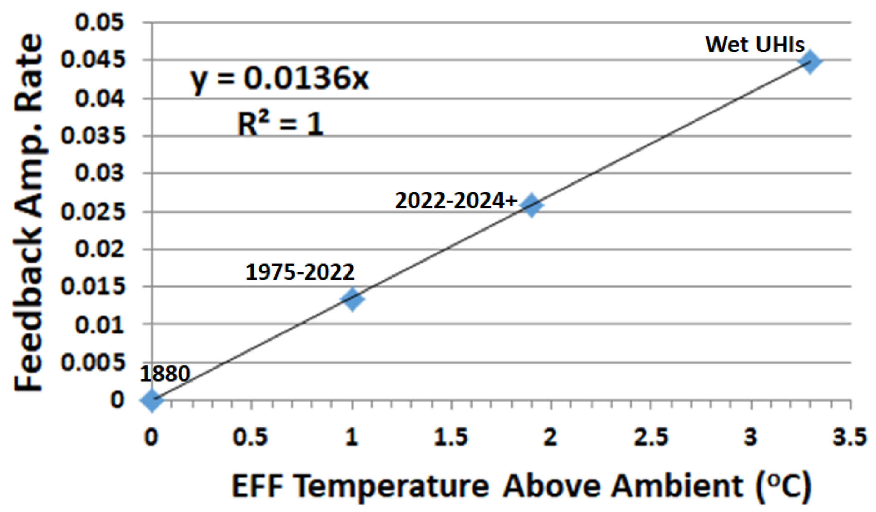
3.5. A_{Feedback Amp} Characteristic Temperature Rate of Change and EFF Temperatures and Urbanization Issues

In the pre-industrial (1880–1900) period, feedback was negligible. Over the years, it has slowly increased due to forcing, feedback, and feedback loops. Here, we look at a graphical method to estimate the rate of change of the feedback slopes with temperature in Equation (10) to gain insights, where

$$\boxed{{\displaystyle \frac{d{A}_{Feedback amp}}{dT}}\approx {\left({\displaystyle \frac{d{\left(\frac{\mathsf{\Delta }{T}_S}{\mathsf{\Delta }t}\right)}_{NCR}}{dT}}\right)/\left({\displaystyle \frac{\mathsf{\Delta }EC}{\mathsf{\Delta }t}}\right)}_{NCR}}$$

(22)

We know that the positive feedback and related loops’ rates are related to environmental temperature changes. Therefore, we can study how the characteristic temperature forcing rates subtlety change feedback over time with the assumption that it might help us understand the behavior of feedback and feedback loop trends that are degrading our climate, due to increasing forcing temperatures. Although we think of feedback events on a global scale, there are also related micro-climate urban problems. We can see from Figure 8a,b that feedback amplification changes over time. The reason is primarily temperature driven by GW increases over land and oceans.

We would like to use as much data as possible. Therefore, we can look to incorporate not only the forcing feedback rates of change in Figure 8a,b but add both the pre-industrial zero data feedback point, as well as UHI feedback observations related to a study by Zhao et al. [9] and Feinberg [10]. In the Zhao et al. [9] study, it was found that UHIs in humid (or wet) climates are 3.3 °C hotter than roughly equivalent UHIs in dry climate areas [9]. Other authors have considered exponential modeling for positive feedback loops [44] and this is has been used in Figure 8c,d. However, in overviewing the data for this section, this graphical approach appears to indicate simple linear behavior (Figure 11). That is, the data used in this section’s study, and the way they are modeled here, do not lend themselves to exponential behavior. The simple graphical solution shown in Figure 11 yields an effective forcing feedback temperature model with the following characteristic.

$$\boxed{\mathrm{EFF} \mathrm{Rate}=(0.0136/\mathit{°}C)(T_2-T_1)}$$

(23)

In this characteristic EFF temperature model, the effective forcing feedback (EFF) rate is the graphical method for finding the temperature derivative of the slopes in Figure 8a,b with the help of two other extra data points that we discuss. The slope is then the graphical estimate of the EFF rate of change, with an observed slope value of 0.0136/°C as a function of temperature. Note that the slope is also characteristic of the Figure 8a slope. Here, T₁ is the average temperature of the Earth, taken as T₁ = 14.5 °C. T₂ is taken as the characteristic EFF temperature. The value T₂ − T₁ was adjusted for the linear fit so that all values optimally yield an R² = 1 data fit (see Figure 11), with the restraint that the feedback amp. rate equates to Figure 8a,b slopes and additionally must pass through the pre-industrial zero point. The characteristic forcing feedback temperature T₂ − T₁ values are then optimally found.

Table 4. Positive feedback loop effective temperatures and FFR amp.

Average Weighted GW Temperature Rise * (°C) (Period)	Avg. Weighted Land GW Temp.** Above T1 (°C)	Model Results EFF Temp. T2 − T1 (°C)	EFF Rate Model Equation (23) (X = EFFT) (°C/Yr.)
0 Pre-industrial	0	0	0 Modeling restraint
1.01 × 0.6 = 0.6 (60% weighted) (1900–2022)	1.05 (=0.6 × 1.74)	1	0.0136 (Figure 8a) Modeling restraint
1.28 × 0.6 = 0.77 (60% weighted) (1900–2024)	1.33 (=0.77 × 1.74)	1.89	0.0258 (Figure 8b) Modeling restraint
0.6 (1900–2022)	1.04	3.3 (Humid UHIs)	0.0449 (Humid UHIs)
0.6 (1900–2022)	1.04	4–15 (Roads, roofs)	0.0544–0.204 (Hydro-hotspots)

** Appendix A, * estimate, 1.74 × GW = average land temp.

shows the model’s results for various estimated T₂ − T₁ values in the period studied. The last row is provided for discussion.

In Table 4, the characteristic EFF temperature rise is given by T₂ − T₁ (temperature value above ambient) for an observed period. So, it is a characteristic value for that period. Here, the model’s slope is an optimum fit in columns 1–3 and rows 1–3. Note the use of the pre-industrial zero point. In Figure 8a, we can see that the EFF temperature for 1900 to 2022 is 1 °C above ambient for an R² = 1.

We can use a weighting estimate of 60% over the time period, yielding a global warming average of 0.6 °C. Land temperatures are about a factor of 1.74 higher than the GW average. Here, the GW slopes to the GW land slope are used for this estimate (see Figures 2 and 3 in Ref. [5]). Thus, the average land temperature over this period (1900–2022) is about 1.05 °C (1.74 × 0.6 °C), and is 1.33 °C (0.77 °C × 1.74) for the period of 1900–2024.

3.5.1. Interpretation of the EFF Temperature

There are several possible interpretations of the EFF temperature characteristic found in Table 4: (1) a characteristic EFF temperature of the feedback processes and their loops, (2) the EFF temperatures (1.0 °C to 1.89 °C) is closer to the GW land temperatures, possibly indicating that urbanization forcing may have more significance than previously thought, and (3) it may be an indication of pipeline warming to come. Interestingly, Scenario 2 involves both Scenario 1 and 3. We note land temperatures are about twice as hot as over the ocean. Land temperatures are increasing at a rate of 2.7 times faster than ocean temperatures. Thus, land temperatures in this view, are significant in driving global warming, pipeline issues, and possibly feedback problems. This warming is primarily due to the ocean’s heat capacity, with other contributors of albedo snow and ice loss, deforestation, and urbanization warming are primary issues. We have noted the contributions of urbanization in Section 3.4.

We can see that the EFF temperatures are closer to the 60% weighted land temperature averages over their respective periods in Table 4 rows 2 and 3. We can investigate this interpretation. It suggests that the model’s characteristic EFF temperatures indicate that land may be more influential than the global average for feedback, which is dominated by water vapor. That is, it is not uniformly distributed as one might expect from CO₂ forcing due to land’s higher GW temperatures. Alternately, this may not be surprising as the land’s GW atmospheric temperatures are known to be hotter than over the ocean, and warm air holds more water vapor. However, we know from satellite data that most of the water vapor is in the tropics [6,45]. Yet, feedback is dominated by forced WVF. This appears to suggest some forcing issues may occur over land. If so, the main forcing would be related to urbanization.

3.5.2. Interpretation of the UHI WVF and Hydro-Hotspot Issues

In row four of Table 4, the UHI temperature is fixed at 3.3 C, which is the increase for UHIs in wet climates reported by Zhao et al. [9]. Therefore, this value if fixed. The model’s result that falls on the R² = 1 line is in this case the feedback amp. rate of 0.0449/°C. Note that this value is about 1.74 to 3.3 times higher than the feedback amp. rate of rows 2 and 3 of Table 4. The 1.74 factor is close to the value found in Equation (17).

Feinberg [10] found high water vapor feedback of over two times that of the background climate, indicating this possibility. In that study, Feinberg [10] provided high water vapor feedback estimates of 3.1 Wm² K⁻¹, 3.4 Wm² K⁻¹, and 4 Wm² K⁻¹ for 5 °C, 15 °C, and 30 °C average ambient UHI temperatures, respectively. We can compare these to Equation (17), which shows the higher UHI water vapor feedback 2+ increase compared to the background estimates. Additionally, it is also estimated that about 75% of the world population is considered to live in humid climates [46,47].

Lastly, we consider the problem of hydro-hotspots. This is defined as water vapor created during precipitation from surfaces above ambient, in this case, 4 °C higher than ambient. These hydro-hotspots induce rapid temperature changes during precipitation and humid periods. Numerous pavements have temperatures that far exceed this. We note that urban local water vapor feedback may not have feedback loops. We can see that UHIs may have very high amplification above the baseline climate. That is, UHI effective ERF is likely more significant than is considered by most climatologists relative to the GW issue. Climatologists who study ECS, other than this study, assume a negligible urban impact. Therefore, urbanization may be making some possible significant GW feedback contributions, as indicated in Section 3.4.

Conservative mitigation in this study and prior work [25] indicates the need to implement, at the Paris Agreement level, albedo requirements for all impermeable surfaces. Mitigation of T₂ − T₁ high-temperature surfaces (Equation (22)) should be a worldwide requirement. There are not enough studies that take into account urban water vapor feedback, and albedo requirements are common-sense safeguards and part of proper solar geoengineering. Currently, negative solar geoengineering of dark roads, roofs, building sides, and even cars dominates our everyday lives. There are no safeguards in the Paris Agreement to prevent negative solar geoengineering.

We do not know the full impact of negative solar geoengineering, as indicated in this section. Feinberg [14] illustrates that one acre of a black road or roof in the Sun equates to the equivalent energy of 74,000 gallons of gasoline per year (gasoline-resulting heat if it were on fire) or is equivalent to 7.5 times more energy than a solar power plant produces per acre. This, combined with hydro-hotspots, results in unknown climate warming issues and merits mitigation methods.

3.5.3. Aerosols and Urban WVF

The IPCC places a high level of reverse effective radiation forcing on aerosol, with an ERF of about 8–10% relative to the estimated total forcing. We note that aerosols last in the atmosphere for hours to a few days. In comparison, similar-sized cities in dry and wet climates create UHI heat and high water vapor feedback from hot impermeable dark solar-heated surfaces of streets, rooftops, building sides, and cars, as found in prior studies [9,10,25]. This humidity by comparison lasts on average 10 days, much longer than aerosols. Furthermore, for pavements and rooftops, solar heating does not have a lifetime like aerosols. It is confusing how studies and the IPCC place strong forcing significance on tiny aerosol particles with short lifetimes but claim with high confidence that urbanization does not influence GW, in the presence of opposing studies [25,26].

3.6. Global Warming Mitigation and Modeling EC and IPCC ERF Issues: Population Control and Trying to Achieve IPCC RCP CO₂ Reduction Goals

The world population growth is slowing, and we may eventually achieve zero population growth and even a decline in the world population. This is anticipated to possibly occur by 2075 [46]. It is interesting then to try and estimate the effect on GW due to zero population growth and its effect on CO₂ and energy consumption reductions.

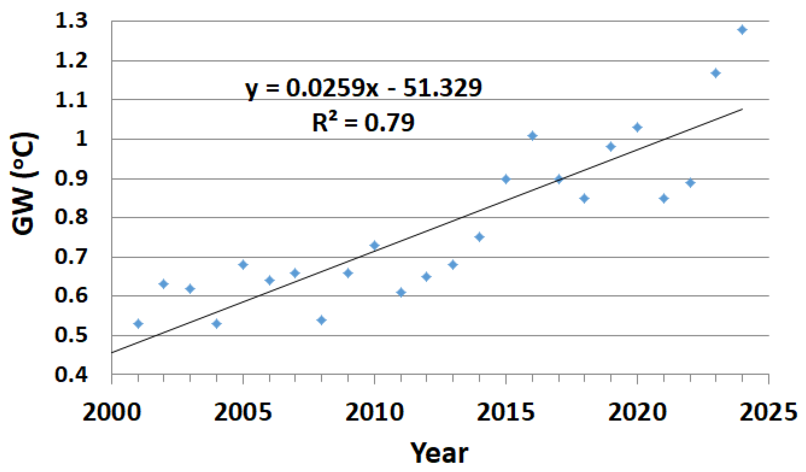
Unfortunately, there is little data to support predictions. Appendix F, for example, plots the raw GW data from 2000 to 2025. The years 2008–2009 and 2020–2021 were interesting as there were strong reductions in EC that occurred. In 2008–2009, there was a financial crisis with a 20% reduction in EC. This compares to atmospheric CO₂ levels, which appear to drop by about 23% compared to the year 2007 in Appendix A. In 2020, COVID-19’s influence yielded an EC reduction of 14% (see Appendix F). However, atmospheric CO₂ levels appeared to increase at the same rate as the year 2019 (see Appendix F). Note that CO₂ atmospheric levels are more complex than EC changes. For example, we anticipate that CO₂ emission rate changes will occur as the EC rate changes. Yet, atmospheric levels are also made up of natural CO₂ contributions like wildfire CO₂ increases, which, in many cases, can be considered a form of feedback. Additionally, deforestation is a form of CO₂ forcing increase, which, while recognized, is not estimated in IPCC ERF (see Table 7.5 in Ref. [32].

Table 5. Categorizing CO₂ sources and modeling issues.

CO2 Sources	Forcing	Feedback	Tabulated in IPCC AR6 ERF (Table 7.5 in Ref. [32])	Accounted for in the EC method
Anthropogenic emissions (CO2 & Methane, etc.)	√	X	√	√
Deforestation	√	X	X	√
Wildfires	X	√	X	√
Volcanic eruptions	X	X	X	√
Decomposition of organic matter	X	√	X	√
Ocean release	X	√	X	√
Anthropogenic waste heat	√	X	X	√
Urbanization construction	√	X	X	√
Wars	√	X	X	√

Since the EC graphical method takes into account both EC and global warming with its ratio (Equation (10)), most contributions in the feedback are accounted for (last column).

illustrates the ERF complexity for EC comparisons to CO₂ atmospheric levels and IPCC ERF estimates. Note that the last two columns show the EC method is believed to incorporate more CO₂ feedback sources in the ratio for the Equation (10) model.

In terms of GW changes relative to EC and CO₂ changes, it is interesting to note that there was a large drop in GW in those periods (see Appendix F). However, these data points are confounded by a moderate La Niña in 2021 and a weak La Niña 2008–09 [48]. This makes it difficult to provide definitive conclusions regarding how perhaps zero population growth might affect GW trends. Theoretical estimates that were initially done in this study were mixed for the EC and CO₂ approach as CO₂ atmospheric increases are complex, as shown in Table 5. However, since GW is related to population growth, it is reasonable to still recommend population control as an additional mitigation strategy.

It is apparent from Table 5 that CO₂ increases even during years of significant EC reductions are problematic, as emissions, even if controlled, other sources can and will cause contributions like wildfires, deforestation, and wars. In addition, not all countries (now including the U.S.) are participating in the Paris Agreement.

This may make it increasingly difficult to achieve RCP near-term and possibly long-term levels. Given the pace of GW and the FD strength, we should conclude that solar geoengineering as a mitigation strategy has become critical. Further studies on these topics will be helpful.

4. Discussion: Recent Trend Analysis for CO₂, Feedback, and Global Warming Due to High Water Vapor Trends

Recent NCRs for the last decade can be compared to the period from 1975 to 2022 in

Table 6. Recent trends in NCRs compared to the 1977–2022 history.

	Column →	A	B	C	C/B
Row	Approx. Years	CO2 NCR Per Year	EC NCR	GW NCR Per Year	Feedback Amplification
1	2013–2025 (2018)	0.0273	0.0122 (2011–2021)	0.0224–0.029 *	1.84–2.37 *
2	1975–2022 (2000)	0.0209 (Figure 7)	0.0124 (Figure 6a)	0.0204 (Figure 6a)	1.65
3	(Row 1-Row 2)/Row 2	30%	0.984%	10%

* Figure 6a ’s 2013 to 2023 adjusted, pipeline trend (Hansen et al., [34]).

. We note that the GW NCR slope of 0.0204 Yr⁻¹ in Figure 6a,b for the years 1975 to 2022. When this is refined to data in these figures for the period of 2013 to 2022, a GW NCR of 0.0224 Yr⁻¹ is found, which is an increase of about 10%. Table 2 also incorporates pipeline assessment due to Hansen et al. [34], which estimated an increase in the GW rate from 0.02 °C/year to 0.027 °C/year. When this is adjusted to an NCR slope, the value yields 0.029 Yr⁻¹. This is an increase of about 42% from the GW NCR of 0.0204 Yr⁻¹. In Table 2, Column C’s ratio to Column B for the EC approach yields the feedback amplification values in the last column. These values can be converted to feedback units, as illustrated in Section 3.2. We note that feedback amplification similarly jumped for 2024 from 1.65 to 2.37. This is about a 44% jump and it is related to the GW NCR jump. We can see the jump in Figure 8b, indicating nonlinear behavior. This point occurs in a very short time period. Lastly, this feedback jump is observed disproportionately in NOAA [49] stratospheric water vapor estimates in Figure 12, which shows an overall jump of 775% in the upper stratospheric data from 2022 to 2024. This large jump was thought to be related to the volcanic Hunga Tpnga-Hunga Ha’apai eruption. However, a study by Schoeberi et al. [2] has suggested that this might not be the case, which leaves this jump somewhat unexplained.

We note that the energy consumption rate had a small decrease of about 1.5% (from 2011 to 2021), indicating that, in general, forcing should not be the main reason for the nonlinear activity. This is because we have shown that the EC NCR showed approximate equivalency to the forcing NCR in Section 2.1. The atmospheric rate of CO₂ increase is about 49% for the linear slope from 2002 to 2022 compared to the slope from 1975 to 2002 in Figure 9. However, this does not account for the jump in data from 2022 to 2024. The increase in CO₂ was about 5 ppm in this period out of 420 ppm, which is only a 1.2% increase. Therefore, the nonlinear activity may be related to high feedback behavior due to the strong El Niño that occurred.

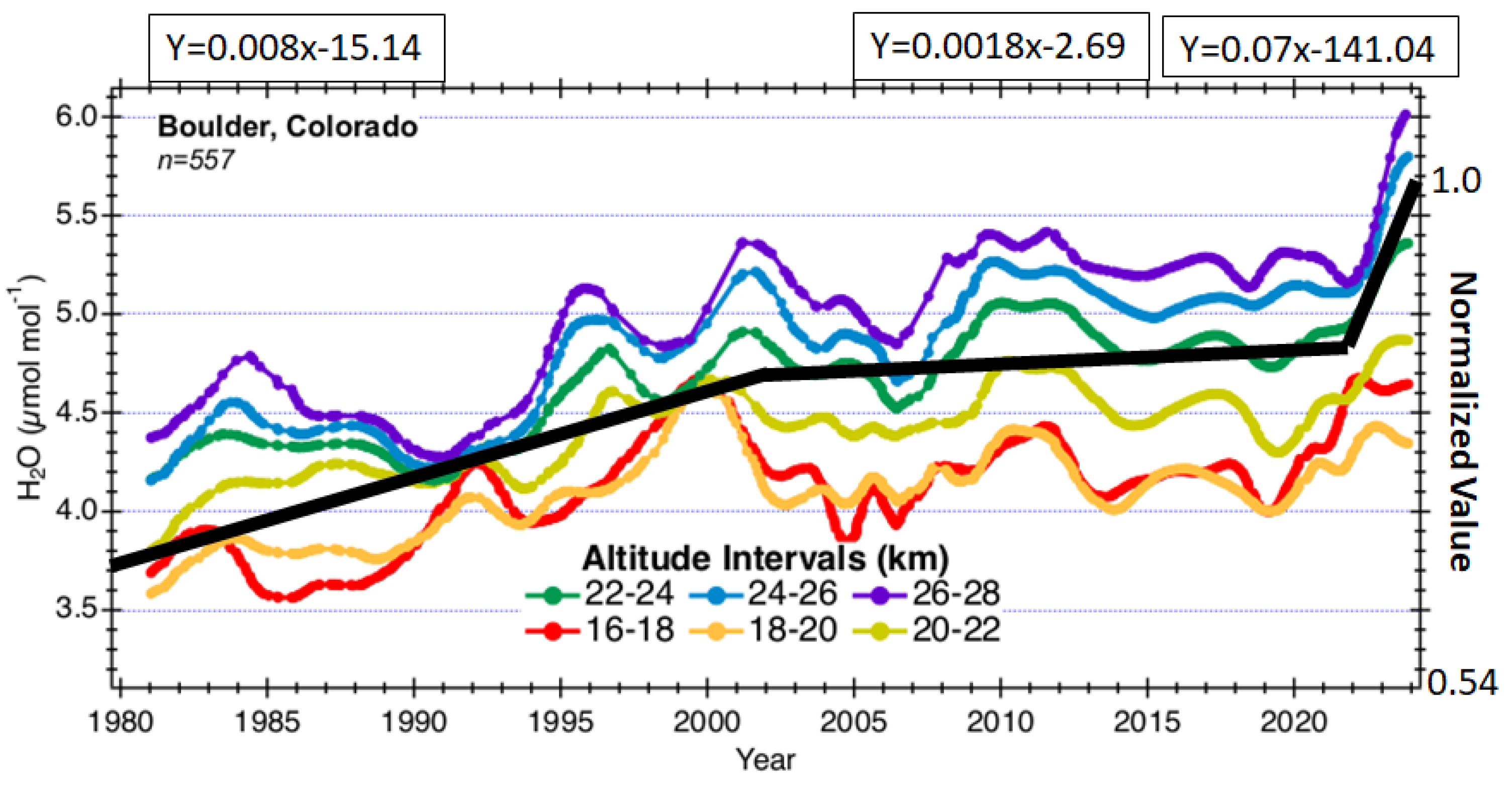
It is helpful to study Figure 12 in more detail. Stratospheric water vapor (1980–2024) is known to help assess the Earth’s climate system affecting atmospheric and surface temperatures. Black trend lines have been added in Figure 12 to the NOAA [49] data providing changing slope estimates. The normalized slope from 1980 to about 2002 has an NCR of 0.008 Yr⁻¹ (Figure 12, see top box) and from 2002 to 2022 has decreased to 0.0018 Yr⁻¹, a 78% reduction; then, a marked increase is observed from 2022 to 2024 to 0.07 Yr⁻¹, a jump of 775% in the NCRs from the 0.008 Yr⁻¹ value.

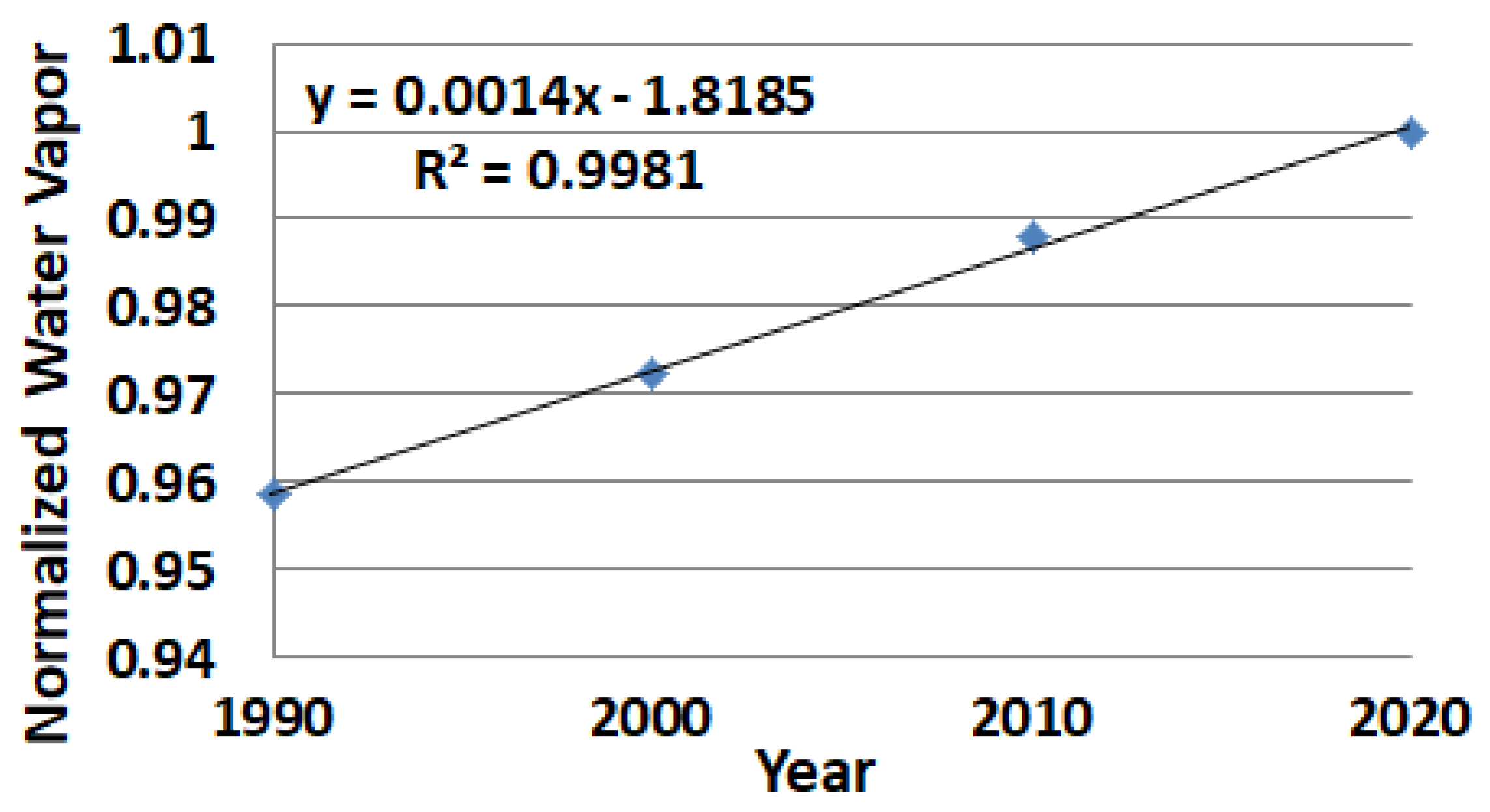
It is helpful to note that Figure 12 period from 1990 to 2020 with stratosphere NCR of 0.0018 Yr⁻¹, compares well with Figure 13, showing the troposphere NCR of 0.0014 Yr⁻¹ extrapolated global water vapor average (extrapolated from Patel et al. [45], with the land and ocean weighted 70% ocean and 30% land). This lends support to the notion that Figure 12’s stratospheric observations are relevant to tropospheric behavior, providing helpful climate insights.

4.1. Observations of Water Vapor Increase Correlated to Global Warming Increase

From Figure 13, we can see an increase in troposphere water vapor from 1990 to 2020 of 4.3% (={1 − 0.9586}/0.9586). From the smoothed data in Appendix A, we note a global warming increase from 1990 to 2020 is 0.59 °C (=0.92 °C − 0.33 °C). For every 1 °C atmospheric rise in global warming, the atmosphere can hold about 7% more water vapor. GW in this time period shows that a possible 4.13% (=0.59 × 7%) water vapor increase may be expected. Results show that the tropospheric atmosphere has in fact increased its water vapor content to the predicted amount, confirming the warming influence.

4.2. Solar Geoengineering for the Arctic and Antarctic to Limit Global Warming

The Arctic and Antarctic are atmospheric heat sinks that help cool the planet. Heat flows from hot to cold areas according to the second law of thermodynamics. Therefore, as the Arctic and Antarctic warm, the amount of heat that flows out of the planet in those areas decreases. Eventually, the Earth will overheat and other effects like ocean levels will rise and cause an unlivable planet. Additionally, the ice-albedo feedback loop effects add to the warming problem, as reflective snow and ice are lost.

In non-Arctic areas, re-radiation has increased. The pre-industrial re-radiation level in these areas was about 61.8%, with 38.2% of heat escaping to outer space [13]. However, with the increase in water vapor, which is close to the FD threshold in 2024, the amount of heat escaping in non-Arctic areas due to this new background climate is likely down to 35.5% [13]. This is not the case in the Arctic areas, as cool air holds less water vapor. The likely amount of trapping heat is not well established in Arctic areas, but it is likely around 45%, with possibly as much as 55% of heat escaping to outer space.

However, if the Arctic and the Antarctic were maintained so the amount of heat escaping into outer space was at current or possibly back to pre-industrial levels, even if the rest of the Earth had large amounts of GHGs, the Earth’s GW temperature rise should be limited, and major Arctic tipping points would also be avoided {52]. The current problem is that the Arctic and Antarctic are warming at a rate of 2–3 times faster than the global average, with the smaller Arctic warming the fastest.

There are several proposed SG methods to help save the Arctic. The main one is SAI [15]; this can be carried out in the summer months, which would allow time during the winter months to prepare [15]. If we start small, applications could provide reversal effects in the near future. As it takes time to build a proper aircraft fleet and logistics, so major applications are likely 10 years away [15]. SG will likely encourage albedo-Arctic feedback loop reversals, which could reduce the amount of SG required.

A second method is the manufacture of synthetic ice cubes. These would be shiny floating cubes placed in calm water areas to reflect the Sun’s energy away, reducing ice melting in the summer months.

Other methods have been proposed like increasing ice thinness in the winter by pumping Arctic water on top of thin ice areas to thicken it.

We can conclude that saving the Arctic and Antarctic is required to help save the planet, and these areas are leading candidates for SG.

4.3. Mild Solar Geoengineering Mitigation Requirements: Pushback Confusion and Risk Assessment

This paper recommends mild solar geoengineering [5] due to aggressive GW increases (Figure A1), feedback now estimated to have exceeded forcing by 8% (Figure 1), and the lack of progress in CO₂ reductions which has many sources contributing to atmospheric levels other than emissions (Section 3.6 see Table 5). Reverse forcing requirements are quantified in Table 3, and it is suggested that Annual Solar Geoengineering (ASG) methods [5] should be used to help stabilize climate feedback. It is important to realize that the longer we wait, the more impossible the SG task, as indicated by Table 3’s reverse forcing requirements to stabilize feedback. Therefore, efforts should be started, using a mild annual approach [5] with a multi-facet method, including Earth brightening, space sunshading, and SAI. Since we have passed the FD threshold, it appears reasonably necessary for climate mitigation. Unfortunately, pushback by Biermann et al. [50] and the Saami Council [51] was largely responsible for stopping a major recent solar geoengineering study by Harvard in 2024 [52] called the Stratospheric Controlled Perturbation Experiment (SCoPEx).

Regrettably, these pushback efforts have provided a high level of confusion about the consequences of SG and provide excuses for governments to avoid spending money on SG methods. The pushback efforts are based on unrealistic high-risks SG reversals and are unclear and confuse SAI with even simple Earth brightening. They appear to oppose all forms of SG according to their title {50]. Such studies are those of an extremist position [50], with biased reviews. Published findings of this nature are unproductive. Claims are made based on theoretical academic unrealistic situations. They also do not understand how much more efficient SG is compared to GHG removal and have been ill-advised.

Such studies and petitions are highly misguided and provide misinformation based on unrealistic fear factors. This published paper [50] and petition are unrepresentative of the current knowledge base reality and are unprofessional and poorly written and reviewed. It has seriously hurt development chances which takes 10–20 years to provide helpful solutions. In short, GHG mitigation without SG leaves us with life-threatening issues that these studies have not addressed and appear to be making inconsiderate misinformed decisions for 8 billion people’s lives that will be at stake.

For example, a mild approach, which is feasible and realistic, such as an annual solar geoengineering approach recommended in this paper, is a factor of 50× less severe and 62% more efficient (see Appendix B.3, [13]) than GHG removal which is difficult to remove. A yearly increase in GW is about 0.02 °C to 0.027 °C, and full mitigation is about 1.3 °C currently. An annual SG approach would involve 50× less effort (about 2% of GW) to try and stabilize the climate. However, because of these pushback efforts, any mention of the word “solar geoengineering” is now frowned upon because these groups have been highly irresponsible without quantifying SRM methods, severity, and true risks that have not addressed how we can mitigate GW without SG, the most efficient tool.

Furthermore, building an infrastructure for an SAI (one SG method) aircraft fleet for even mild mitigation is realistically 20 years away over the equator [15,53] and about 10 years away in the Arctic [15]. Currently, there is zero effort in this area, and pushback efforts have strongly contributed to the lack of effort with unrealistic consideration for the life-threatening situation on this planet.

Realistically, risk assessments should be responsibly done before publishing. One should consider the equal and opposite extreme positions on the risk of willfully neglecting SG and its opportunity [54]. Risk is the Probability of Failure x Cost. Given the difficulty of GHG mitigation and the fact that there are many natural CO₂ sources other than GHG emissions, such as wildfires, increasing atmospheric CO₂ (see Section 3.6 for the numerous sources), along with the problem of now passing the FD threshold, where feedback accounts for more global warming than forcing, we can see that the probability of mitigation failure has significantly increased; meanwhile, the cost is related to the survival of the human race. Therefore, the risk appears to be extraordinarily high. We can liken this to a house on fire with a fire extinguisher available to stop the fire. If the fire extinguisher is not available, the house will burn down. It is important to have the tools available in emergencies, as is currently the case in our global warming crisis.

Lastly, the FD overage level is estimated up to 3.6% in Table 3. This is significantly higher than the yearly global warming increase of about 2%. If forcing could be removed, we would still have a GW increase due to the FD overage level. This means that without SG, we will not be able to mitigate GW.

Given the difficulty of full CO₂ mitigation methods and the fact that water vapor feedback trends were likely apparent by 1990 (see Figure 12 and Figure 13), one might use the fact that SG has a 62% higher efficiency than CDR (Appendix B.3, Ref. [13]) and is the most effective method. Note that solar heating is the primary warming effect, while GHGs are the secondary effect. Removal of the primary influence also reduces the secondary GHG influence, and is 62% more efficient (Appendix B.3, Ref. [13]). Yet, many climate scientists do not appear to recognize that CDR is 38% (Appendix B.3, Ref. [13]) less efficient in comparison and often view SG as a band-aid solution. This is disappointing and appears confusing since water vapor feedback is reasonably well-understood [3,4] and was even estimated to have doubled the forcing in 2013 by other authors [6,7]; yet, no SG recommendations have been made by IPCC authors other than GHG mitigation.

Furthermore, we are already doing negative SG with dark roads, roofs, cars, and building sides [5,25], which creates concerns given urbanization heat flux studies [25] and our global warming crisis (see Section 3.4). Negative SG causes heat fluxes that are re-reradiated by GHG warming with the same 62% efficiency (Appendix B.3, Ref. [13]).

Goldblatt and Watson [3] noted that the upper water vapor feedback limit is not well-understood and we need all available mitigation tools. Implementing SRM will likely cause environmentally unfriendly issues. However, risks are now extraordinarily high and we need to condense out some of the water vapor ASAP. Additionally, we are already doing negative SG in cities without restrictions, with no Paris Agreement albedo requirements (see Section 3.4). SG practices in all areas including Earth brightening are required, as time is running out, and risk assessments should be considered and weighed.

Therefore, “mild” SRM [5] methods are needed in climate mitigation. To summarize the key reasons for “mild” solar geoengineering as follows:

• This study indicates that the climate has passed the FD threshold, so reverse forcing using SG is needed to help mitigate feedback increases.
• SG has 62% higher mitigation efficiency (Appendix B.3, Ref. [13]) than CDR (in Watt/m² of work) and is the leading candidate for a reverse forcing requirement due to passing the FD threshold.
• SG is not related to fossil fuel legislation.
• SG produces fast results.
• SG reduces the GHG effect including water vapor feedback.
• SG is something we all can participate in by brightening the Earth with cool roofs and roads.
• Increases in water vapor feedback (Figure 12 and Figure 13) indicate there is no time to waste.
• The annual approach reduces circulation issues by approximately a factor of fifty [5], but we need to act as soon as possible.

5. Summary

In this paper, the anthropogenic effects on global warming dynamics were studied through correlation and trend analysis due mainly to NCRs. Feedback estimates were provided using statistically significant highly correlated data covering mainly the period from 1975 to 2024 using an EC NCR method to estimate feedback amplification per Equation (10).

This study provides the following key results:

• Section 2.1 derives and finds that the normalized rate of energy consumption and forcing shows approximate equivalency from 1975 to 2021, providing a graphical means to estimate feedback using NCRs that are more stable and have higher statistical confidence than point estimates.
• The practical use of the feedback amplification metric (inversely related to the common feedback values per Equation (6)) simplifies many GW estimates such as feedback amplification x forcing yields GW (Equation (11)) and the percent of GW due to feedback (Equation (13)). It also simplifies SG background climate estimates (see Equation (21) and refs. [5,25]).
• Feedback amplification can be estimated from Equation (10) and feedback from Equation (12). Section 3.2 shows feedback and forcing assessed in this paper compared well to IPCC AR6 values. Additionally, this paper provides the method to convert feedback amplification value to feedback and vice versa (see Section 3.2 and Section 3.2.1).
• Feedback amplification trend estimates are obtained and plotted in the period from 1880 to 2025 in Figure 8. This is likely the first such trend estimates and definition of the FD threshold (A_{Feedback amp.} > 2) when forcing exceeds feedback (Table 3), assessed to have occurred in 2017. Feedback amplification trend estimates are shown to provide accuracy at the 95% confidence level (Section 3.1.1) indicating that key results will fall within the IPCC likely range.
• From 1975 to 2022, the following rates were observed: The rate of feedback amplification increase is estimated as 0.136 per decade (Figure 8a). The forcing and EC NCR rates are about 0.124 per decade (Figure 4b and Figure 6a). The NCR rate of GW is 0.204 per decade (Figure 6a). These rates increased during 2022 to 2024 [34] (Figure 8b).
• Between 1975 and 2024, feedback amplification was estimated to have increased from about 1.46 to 2.16, a 48% increase, as indicated in Figure 8. Exponential fits (Figure 8c,d) were used for feedback amplification trends from 1870 to 2082.
• About 75% to 91% (83% average) of positive feedback is estimated as due to water vapor (Section 3.2.1).
• FD reverse forcing mitigation requirements are provided in Table 3. Table 3 also provides feedback amplification estimates for several different scenarios (including RCP projections) and estimates the percent of GW due to feedback using Equation (13).
• ECS values using the EC NCR method were estimated between 2.4 °C and 3.07 °C (Section 3.2.3), which are in the IPCC AR6 likely range. This provided feedback estimates of 1.55 Wm² K⁻¹ to 1.21 Wm² K⁻¹ using Equation (20), also in the AR6 likely range. However, in Section 3.4, it is estimated that these ECS values are likely lower by 10.7% due to the GW urbanization effect (not considered by the IPCC), which would reduce the ECS likely range between 2.14 K and 2.74 K.
• Table 5 in Section 3.6 illustrates other CO₂ sources besides emissions (which do add to the CO₂ mitigation difficulty) and also illustrates the advantage of the EC model, which may do a better job of estimating feedback. A discussion in Section 4.3 indicates the implications of surpassing the FD threshold, which recommends reverse forcing, for which mild solar geoengineering [5] is needed to avoid the high risks in GW mitigation. Table 3 quantifies the amount of reverse forcing that will likely be required to mitigate the percentage of FD overage level.
• The study has also explored population control as a mitigation strategy (Section 3.6) and CO₂ reduction issues (Section 3.6 and Appendix F). While it is logical to recommend population control, data were not available to support this strategy. CO₂ reduction has proven complex as there are numerous sources not related to emission efforts, making it somewhat problematic in achieving goals, as detailed in Section 3.6. As not all countries are participating in the Paris Agreement (now including the U.S.), indications are that IPCC RCP’s near and possibly long-term goals, as detailed in Section 3.6, will be difficult to meet, making SG necessary.
• In Section 3.5, the feedback amplification rate of change with temperature was investigated. The results provide EFF characteristic temperatures of up to 1.9 °C with several interpretations: (1) a characteristic EFF temperature of the feedback processes and their loops, (2) the temperatures found were closer to the GW land temperature, indicating that urbanization issues can be significant and are SG candidates, and (3) EFF temperature may be an indication of pipeline warming to come. The land interpretation, which is not well studied, was overviewed, adding to the thesis that urbanization albedo requirements should be a major part of the Paris Agreement.
• It is shown in Section 3.6 that the EC approach has many advantages as it incorporates many CO2 and general sources (Table 5) that can be hard to categorize in assessing feedback trends, providing modeling advantages.
• In Section 4.2, it is recommended that we need to save the Arctic and the Antarctic using SG to help limit GW temperature increases.
• The bottom line of this study is that, feedback has become a more significant contributor to GW than forcing by 8% in 2024 (Figure 1). We should not expect that removing all forcing will fully mitigate GW, since it is estimated that we passed the FD threshold in 2017. The 2024 FD overage is 3.7% (Table 3) and is increasing at about 3.1 to 3.9% per decade (Table 3). Results of the study combined with the complexities and failures of GHG reductions, unfortunately lead one to conclude that SG is a mitigation requirement according to the risk assessment in Section 4.3.

Other helpful findings of this study are the following:

• Estimated correlations:

  ◦

  99.3% between population growth and energy consumption increase.

  ◦

  93.4% between energy consumption and global warming (unsmoothed data).

  ◦

  94.4% between population growth and global warming (unsmoothed data).

  ◦

  94.5% between global warming and CO₂ increase.

  ◦

  99.7% between energy consumption and CO₂ increase.

• Estimated rates:

  ◦

  Energy increase per year averages 2183.7 TWh/Year (Figure 2).

  ◦

  Population growth averages 0.084 BP/Year (Figure 3).

  ◦

  GW has been averaging 0.019 °C/Year (Figure 2 and Figure 3). However, 2023 was about 15% higher than anticipated.

  ◦

  NCRs are 0.0204/year (1975–2022) and 0.0224/year (2013–2022) for global warming, 0.0209/year for CO₂ increases, 0.0107/year for population growth, and 0.0124/year for energy consumption (Figure 5, Figure 6, and Figure 7b).

  ◦

  NCR indicates that energy consumption exceeds population growth by a factor of 1.159 or is about 16% higher.

  ◦

  Feedback amplification dynamic trend analysis indicates that by 2047, for 10 BP, the feedback amplification may reach a value of 2.6, which equates to about 61.7% of GW, which may be due to feedback (Equation (13)). This is based on linear trend analysis.

Statistically, global warming dynamics and feedback are strongly affected by the energy consumption rate driven by population growth. Energy consumption NCR driven by population growth is a key concern since it shows equivalency to forcing NCR, as it is strongly correlated with fossil fuel consumption, GHG increases, anthropogenic heat release, black carbon problems, and urbanization issues, all affecting global warming.

The normalized correlated data slope analyses for GW and EC provide statistically significant lines of evidence that can be used to help in feedback amplification estimates, which can be converted to feedback values.

The results in this paper suggest the following issues should also be addressed in addition to the GHG reduction effort in the Paris Agreement, to help mitigate climate change:

(1)

Reduce energy consumption to mitigate forcing (Section 2.1).

(2)

This study (Section 3.5) supported by other research indicates the effects of urbanization’s impermeable surfaces are not well-understood and can even influence feedback both locally and globally. It is important to stop negative SG mainly of dark roads and roofs by requiring higher albedos for roofs, roads, building sides, and cars (Section 3.4). Accordingly, it has been argued repeatedly here and by many authors [5,9,10,25,26,40,42,46] that urbanization albedo requirements are needed in the Paris Agreement.

(3)

Add albedo requirements for black roads, roofs, cars, and dark buildings to the Paris Agreement. Here, we include cars to increase SG awareness.

(4)

Population control is recommended (see Section 3.6) as a mitigation strategy.

(5)

Implement mild annual solar geoengineering [5] (Section 4) methods that include Earth brightening, space sunshading, and SAI to reduce climate risks, helping to reduce water vapor feedback (see Table 3 requirements). In Earth brightening, a focus on cooling hotspots (urbanization surfaces and natural hot areas like Death Valley) should produce maximum efficiency. Additionally, cooling areas in the tropics, where water vapor is highest, should be considered. Other methods, including saving the Arctic and Antarctic, are highly recommended to help save the planet [15] from overheating. In Arctic areas, sea mirror (cubes) [5] and/or SAI methods can be performed in a timely manner (SAI in summer months [15]) and will help limit global warming.

(6)

Implementing a mild annual solar geoengineering program [5] is still very challenging and there is a strong need for NASA, Space X, and the Canadian, Chinese, and European space agencies to help develop the technologies required for ASG implementation. It is hard to justify U.S. NASA goals such as going to Mars when our planet is in serious GW trouble and in need of program funding for SG. One trip to Mars equates to 70 trips to the L1 Lagrange point where sunshading is needed or 1000 s of trips to the stratosphere for SAI applications. It is recommended that these agencies answer the call to contribute in the area of solar geoengineering ASAP, as it can take years to develop and implement solar radiation modification, which is urgently needed today.