Article

Sensitivity of Peru’s Economic Growth Rate to Regional Climate Variability

1
Physics Department, University of Puerto Rico Mayagüez, Mayagüez, PR 00681, USA
2
Geography Department, University of Zululand, KwaDlangezwa 3886, South Africa
Climate 2025, 13(10), 216; https://doi.org/10.3390/cli13100216
Submission received: 25 July 2025 / Revised: 28 August 2025 / Accepted: 16 September 2025 / Published: 17 October 2025
(This article belongs to the Section Climate and Economics)

Abstract

The macro-economic growth rate of Peru is analyzed for sensitivity to climatic conditions. Year-on-year fluctuations in the inflation-adjusted gross domestic product (GDP) per capita over the period 1970–2024 are subjected to correlation and composite statistical methods. Upturns relate to cool east Pacific La Niña, downturns with warm El Niño. Composites are analyzed by subtracting upper and lower terciles, representing a difference of ~USD 40 B at current value. These reveal how the regional climate exerts a partial influence among external factors. During the austral summer with southeasterly winds over the east Pacific, sea temperatures undergo a 2.5 °C cooling. Consequently, atmospheric subsidence draws humid air from the Amazon toward the Peruvian highlands, improving crop production. Dry weather along the coast sustains transportation networks and urban infrastructure, ensuring good economic performance over the year. The opposing influence of El Niño is built into the statistics. A multi-variate algorithm is developed to predict changes in the Peru growth rate. Austral summer winds and subsurface temperatures over the tropical east Pacific account for a modest 23% of year-on-year variance. Although external factors and the varied landscape weaken macro-economic links with climate, our predictors significantly improve on traditional indices: SOI and Nino3. Adaptive measures are suggested to take advantage of Southern Oscillation’s influence on Peru’s economy.

1. Introduction

Anticipating regional climatic anomalies will offer a path to more sustainable economic growth as the earth’s limited resources come under increasing population pressure. Advances in environmental observing networks, satellite remote sensing, and coupled data assimilation enable a better understanding of air–land–sea interactions across multiple timescales. Institutional systems make use of monitoring and prediction services to minimize risk from climate variability and anticipate market supply–demand, food and water resources, and downstream consequences—magnified by socio-political instability. Unforeseen weather events that cause infrastructure damage through extreme runoff lead to outward migration toward better living conditions. Although natural disasters undermine the social fabric, recovery creates opportunities to improve resilience.
Gross domestic product (GDP) is often used to quantify economic performance, but contributions from the informal sector are under-represented and appear through consumption taxes. Past El Niño events exhibited a lagged effect on Peru that led to food shortages and an economic downturn 3–9 months later [1,2,3]. Peru’s vast landscape, spanning coastal desert to tropical jungle, equatorial to subtropical zones, and lowland to highland elevations, offers a great variety of geographic conditions, but its proximity to the single biggest driver of global climate variability is a key feature.
Southern Oscillation refers to a zonal dipole in sea temperature and air pressure across the Pacific Ocean that is linked with the global Walker circulation [4]. With the onset of cooling across the equatorial east Pacific (La Niña) caused by intensified easterly trade winds and upwelling, atmospheric subsidence occurs. Subsequent upper-level convergence draws upper westerly winds from the Maritime Continent, forming a zonal overturning circulation. As the Pacific thermocline tilts westward, an ocean Rossby wave propagates slowly across the basin, taking over three years to reflect and sustain a rhythmic oscillation [5]. Peru’s coastal upwelling plume forms the base of the Pacific cold tongue that stretches from 80W to 120W.
The subtropical anticyclones driving the Pacific gyre circulation are quite intense, but the high pressures relax at 3–7 year intervals in conjunction with a downwelling ocean Kelvin wave [6]. The equatorial currents turn eastward, and warm seawater circulates toward the coast of Peru, bringing heavy runoff [7]. The warm phase of the Southern Oscillation (El Niño) takes hold in the Jan-Mar season, flooding the coastal plains north of Lima (12° S) and disrupting transportation networks. In contrast, El Niño induces drought over the southeastern Peru highlands, leading to crop losses and pasturing scarcity [8,9].
Prior research has evaluated how the Southern Oscillation affects international productivity [10] and Peruvian macro-economic output [3], suggesting a lagged response to opposing phases of the Southern Oscillation that facilitates long-range prediction. Yet questions remain on how the marine and terrestrial climates conspire to induce GDP fluctuations, despite a myriad of external factors [11,12]. This work fills that research gap.
Here, a statistical study is conducted with the aim of determining climatic sensitivity and formulating growth rate forecasts to limit risk and make informed management decisions [13]. Peru is fortunate to have a history of socio-economic metrics and weather observations that lend confidence to our interpretations. In Section 2, the data and methods are outlined, wherein the GDP target is formulated, similar to [14]. Section 3 provides results on (i) GDP growth rate links with Peru climate, (ii) field regressions and composites to establish key climate signals, (iii) validation of a multi-variate algorithm. A concluding discussion is provided in Section 4.

2. Data and Methods

Economic data on Peru’s annual gross domestic product (GDP) was obtained from the Food & Agricultural Organization [15], International Monetary Fund [3], and World Bank in the period 1970–2024. Sectoral contributions to GDP were analyzed, and maps of averaged satellite land and ocean color were calculated. The year-on-year growth rate per capita, inflation-adjusted to constant US$, was averaged over the three datasets to minimize reporting discrepancies. The combined growth rate time series was auto-correlated, lag-correlated with traditional Pacific Nino3 and Southern Oscillation indices, and point-to-field correlated with the Jan-Mar global sea surface temperatures and sea level air pressure. The statistical analysis requires R > |0.26| to achieve 95% confidence with 53 degrees of freedom.
To understand how the regional climate affects Peru’s growth rate, Merra2 reanalysis [16] winds, vertical motion, specific humidity, and air temperature, and Godas reanalysis [17] sea temperature and currents were employed in the Jan-Mar composite analysis 1971–2024. The growth rate time series was ranked to find the highest years: +1986, 1987, 1994, 2006, 2007, 2008, 2010, and 2021, and the lowest years: −1982, 1983, 1988, 1989, 1990, 1992, 1998, and 2020. Thus, the upper and lower terciles were combined and subtracted. Climatic differences were calculated as maps and sections to identify key features driving favorable minus unfavorable conditions using statistical tools from the Climate Explorer KNMI and IRI Climate Library.
From the Jan-Mar composite difference patterns, a pool of eight candidate predictors was extracted, mostly from the tropical east Pacific. Those standardized time series were submitted to multi-variate regression via MS Excel, and step-wise reduced by consideration of p-value and partial coefficient match-up. The outcome was quantitatively evaluated to determine the integrity of forecasts.
The research is focused on climatic links to macro-economic performance and predictability. The scope of work excludes individual sectoral responses, threshold functions, attenuation bias, government intervention, and market forces. In summary, the sequential methodology is (i) formulation of an economic index, (ii) analyzing temporal predictive relationships, (iii) calculating spatial influences via correlation and composites, (iv) inferring climate-resource linkages, and (v) conducting step-wise multi-variate regression to anticipate economic changes.

3. Results

3.1. Peru Growth Rate and Global Drivers

Productivity in Peru is spread across multiple interconnected sectors, as illustrated in Figure 1a. Services account for 35% of the output, whereas agriculture + fisheries yield only 7% yet employ ~20% of the 34 M population. Persistent southeasterly winds induce coastal upwelling, which lifts nutrients. Phytoplankton bloom over the shelf (satellite fluorescence, Figure 1b) and support marine resources. Vegetation exhibits a distinctive response to the Southern Oscillation: La Niña favors crop production in the southeastern highlands (correlation map, Figure 1c).
The Peru total GDP and year-on-year growth rate time series are presented in Figure 1d,e. The total shows little progress over the first three decades, then a steep incline 2003–2013 that has leveled off. Growth exhibits a range of <10%, representing fluctuations of ~USD 40 B (in current dollars) that may be attributed to local environmental and socio-political conditions, and external market forces. The lag auto-correlation of growth rate is R = +0.27 at 1-yr, −0.31 at 4-yr, and +0.17 at 7-yr, suggesting shocks/rebounds and cyclical behavior associated with the Southern Oscillation. Based on the composites presented below, a number of the Jan-Mar climate parameters were tested for covariance with the annual growth rate. Maximum pair-wise R = |0.40| for sea temperature and wind indices in the east Pacific suggest uptake is modulated by the advance and retreat of Southern Oscillation influence across the Peruvian landscape (Figure 1c), and lags between internal and external factors [3].
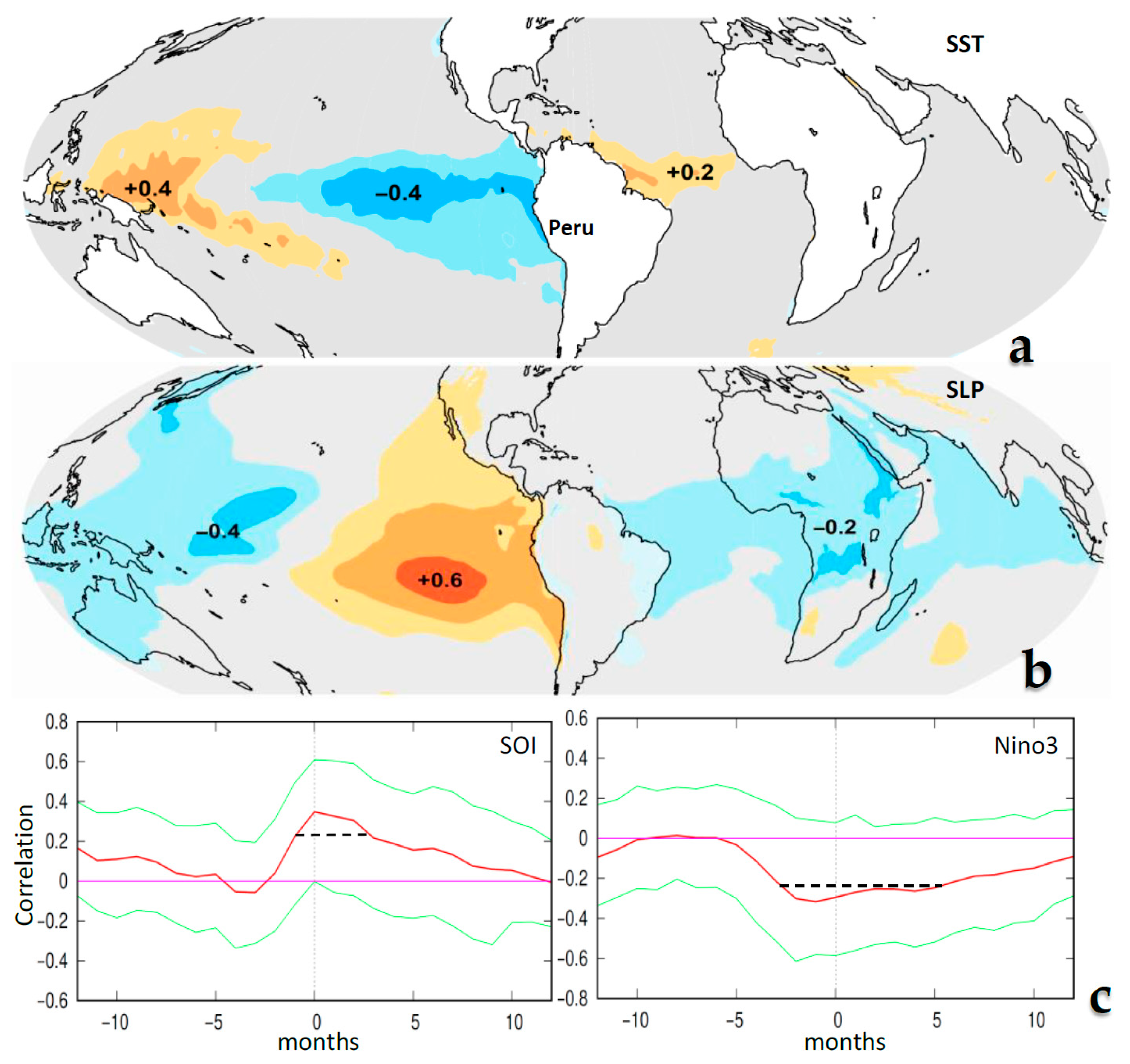
The point-to-field correlation map of growth rate time series onto the Jan-Mar sea surface temperature and sea level air pressure 1971–2024 (Figure 2a,b) reveals Peru upwelling extending to the east Pacific cold tongue. Warmer sea temperatures across the equatorial Atlantic and west Pacific are noted; however, signals are weak across the east Indian Ocean. For air pressure, the opposing dipole pattern emerges: strongly positive over the southeast Pacific, negative over the tropical west Pacific and Africa. The statistics indicate that La Niña favors and El Niño inhibits economic growth in Peru, but the dipole must shift east of the Maritime Continent to create a marked response. That is why lag-correlations with traditional indices: SOI and Nino3 (Figure 2c) are barely significant: R < |0.30| from 0 to 6 months, with the economy following. Thus, risk management decisions would be uncertain, and a more targeted approach is necessary.

3.2. Composite High–Low Growth

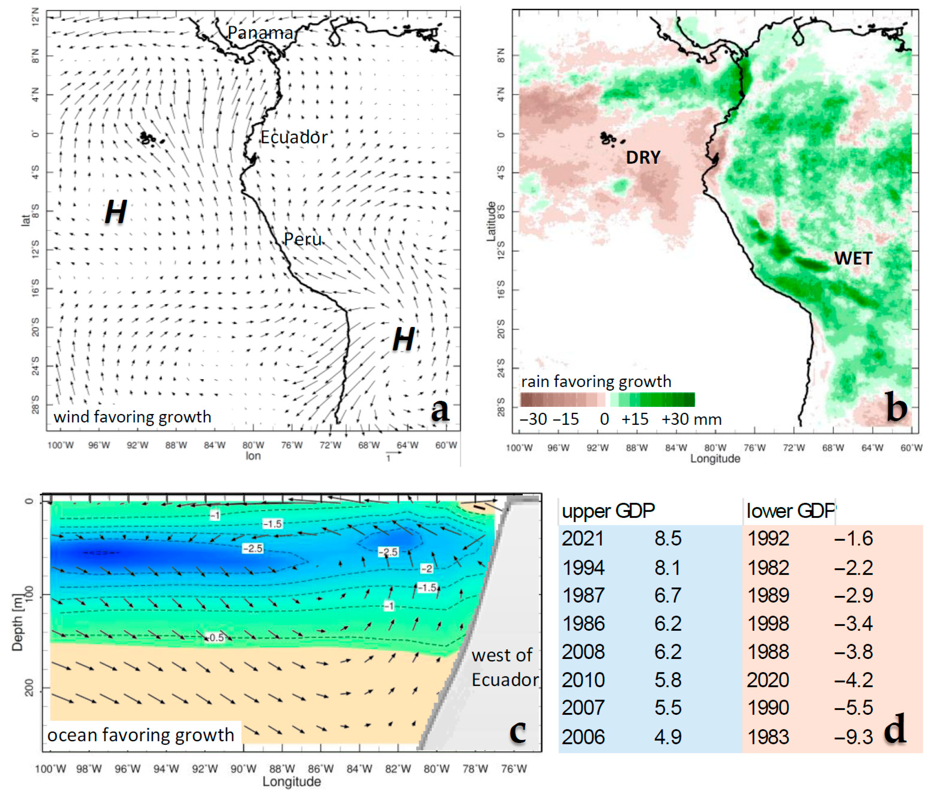
As described earlier, the Peru GDP growth rate was ranked, and the upper and lower eight years were identified. Although economic records commence in 1970, this part of the statistical study is restricted to the satellite era (1980+). Composite maps were calculated for high minus low growth years, focusing on the Jan-Mar season when the Southern Oscillation reaches peak amplitude. Figure 3a–c presents composite difference maps for surface wind, rainfall, and the ocean circulation and sea temperature in the area 30° S–12° N, 100° W–60° W. The winds favoring an upturn in growth are distinctly southerly from Peru to Panama, extending 1000 km seaward. We also note a divergent anticyclone over the Altiplano, locally known as the Bolivian High. Such a circulation is consistent with east Pacific La Niña conditions, which tend to push the equatorial trough toward Central America. Naturally, the opposing El Niño wind pattern favors a downturn in growth.
The composite difference map for rainfall indicates that western Brazil and the Peruvian highlands receive significantly increased summer rainfall prior to higher growth. Decreased rainfall is confined to the maritime zone from Ecuador to the Galapagos Islands at 5° S. The ocean circulation, favoring higher growth, shows an overturning cell with offshore currents near the surface and onshore currents at depth. The subsequent upwelling of seawater induces −2.5 °C cooling at depths 20–120 m off northern Peru. The opposing pattern of downwelling and warmer sea temperatures during El Niño reduces fish catch [18] and causes floods along the coast and drier weather inland. Figure 3d lists those years of high and low growth and associated values. In our empirical analysis, the composite contributions from each year are of equal proportion so as to limit external influences that may alter climate sensitivity, such as the pandemic downturn and rebound in 2020–21.
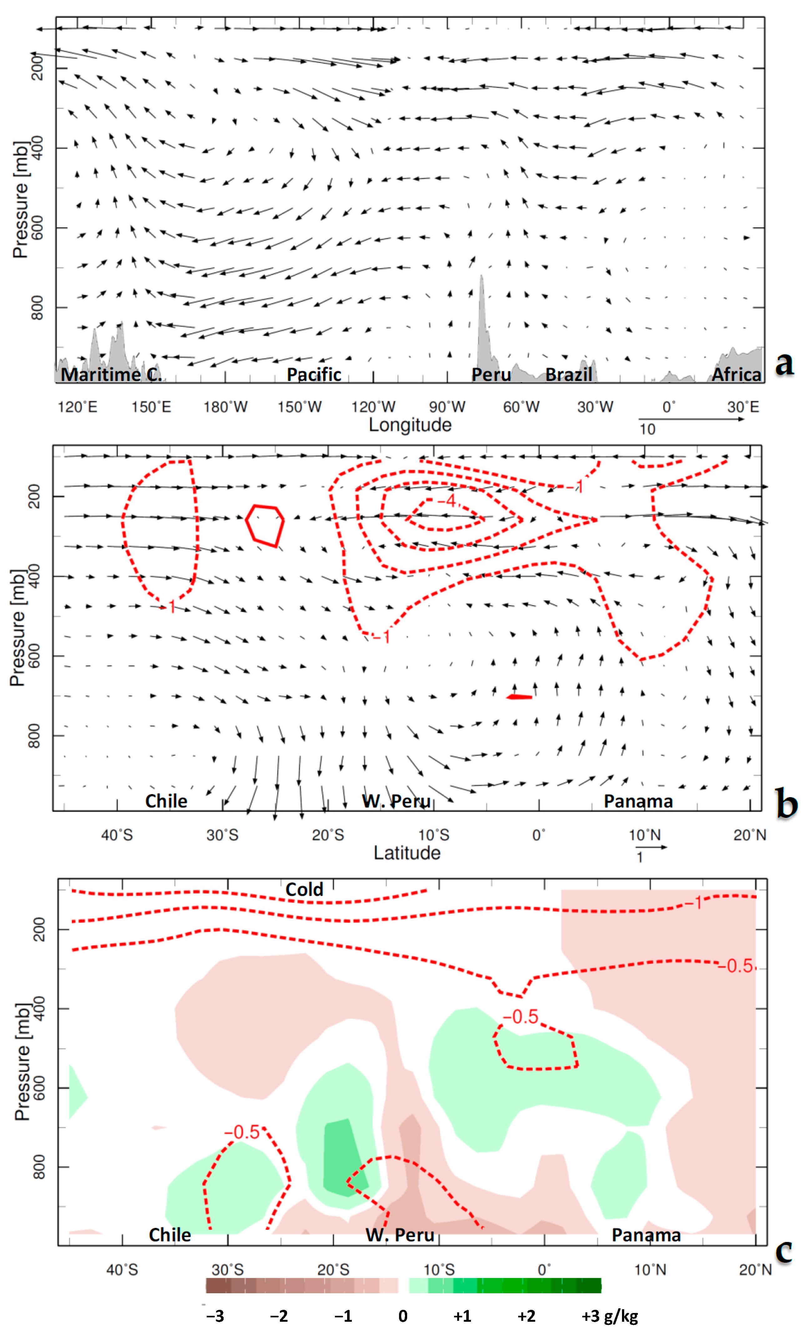
Figure 4a–c presents Walker and Hadley circulation composite differences. The zonal atmospheric overturning (averaged 10° S to 7° N), favoring growth, has easterlies in the low levels across the central Pacific. These tend to sink near 90° W and rise near 180° W, making an arc that draws upper easterly winds from the tropical Atlantic. Upper westerlies appear over the Pacific, completing the Walker Cell associated with La Niña conditions. (There is little circulation response over Africa and the Indian Ocean.) The Hadley meridional overturning circulation (averaged 85° W–70° W) also shows important differences with respect to Peru’s growth rate. Sinking motions are strong over the Peruvian shelf zone, causing dry conditions there. Northward airflow rises near Panama, returning southward in the upper troposphere, completing the Hadley Cell associated with La Niña conditions. We note upper easterly wind differences and cooler air temperatures at 100–200 hPa across the subtropics during years of high growth in Peru.
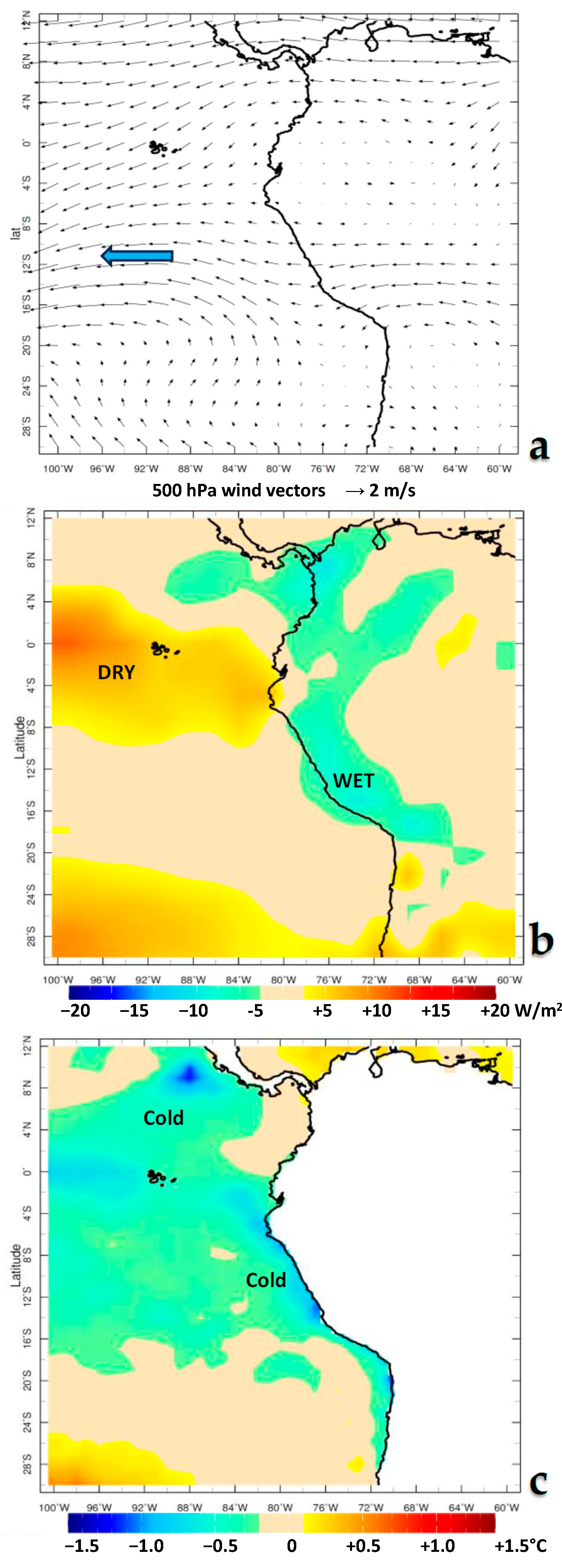
Figure 5a–c presents 500 hPa winds, net OLR, and sea surface temperature composite differences. Easterly winds pour out of the Amazon along 10° S and lift over the Andes, generating orographic clouds (-OLR) that suppress evaporation. Sea surface temperatures favoring growth are cool to the west of South and Central America. Natually, the pattern associated with El Niño is reversed: wet coast/dry inland, with negative macro-economic consequences.

3.3. Multi-Variate Algorithm and Long-Term Change

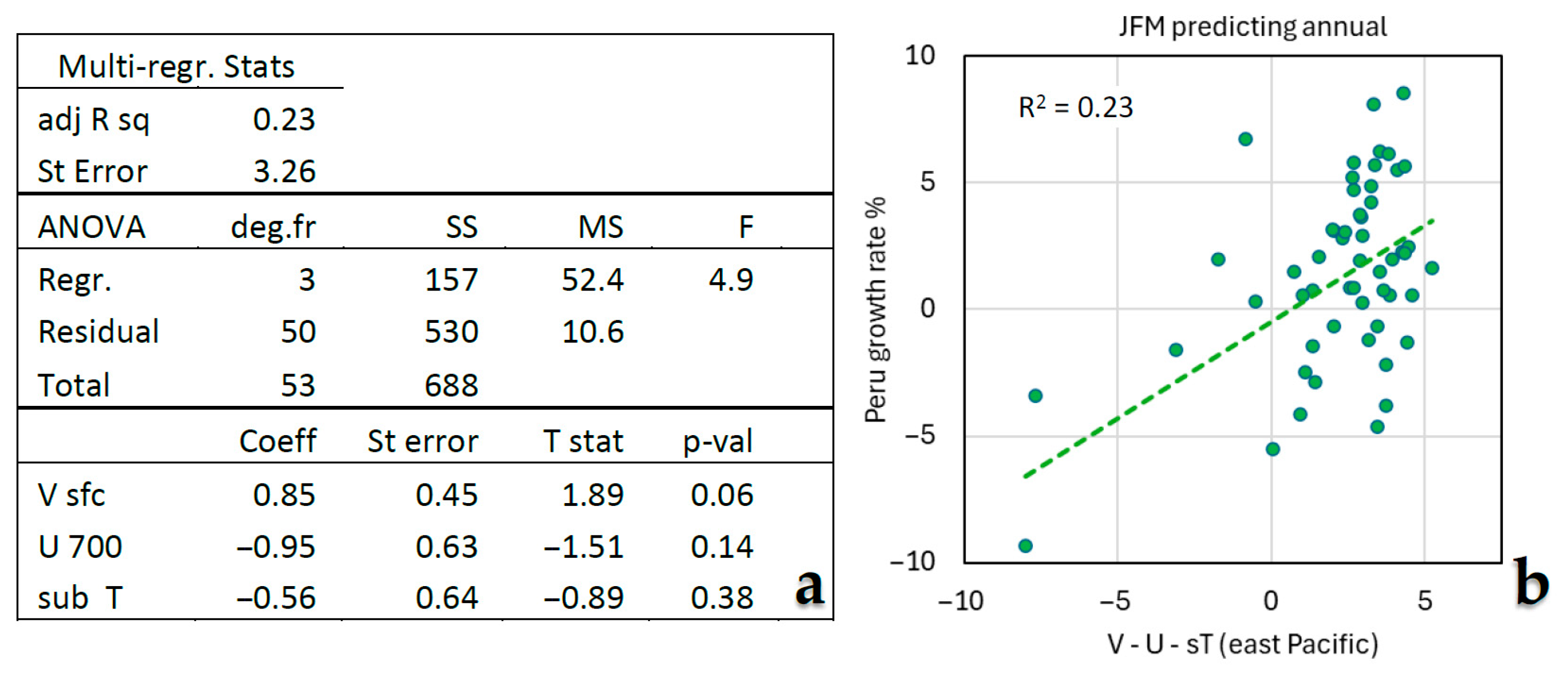
Figure 6a presents a tabulation for the multi-variate regression involving three predictors trained on the Peru GDP growth rate. They include V sfc = meridional wind at 1000 hPa in the area: 5° S–7° N, 100° W–75° W; U 700 = zonal wind at 700 hPa in the area: 10° S–7° N, 180° W–150° W; and sub T = 1–100 m sea temperature in the area: 10° S–7° N, 100° W–75° W. All were drawn from the above composite analysis as the Jan-Mar time series. The meridional wind (from Figure 3a) has the strongest partial influence on growth with p = 0.06; followed by the zonal wind (from Figure 4a), p = 0.14; and then the subsurface sea temperature (from Figure 3c), p = 0.38. Other predictors such as SOI, Nino3, SST, and OLR were eliminated during step-wise reduction.
Unexpectedly, winds ‘out-predict’ sea temperatures. This suggests that the processes driving the Southern Oscillation and its transmission to surrounding countries start with the atmospheric circulation and subsequent uptake by the upper ocean and nearby continents. The scatterplot Figure 6b exhibits a handful of negative values and a narrow distribution of weak positive values. The statistical sample is asymmetric [19]: La Niña is closer to normal than El Niño. The multi-variate algorithm achieves R2 = 23%, which significantly improves on the traditional indices tested earlier. If included with external economic factors, a significant portion of up- and downturns in Peru’s growth rate can be anticipated.
Global efforts to monitor and predict the Southern Oscillation and the long-term impacts of climate change deserve consideration. In situ and remote observations of the marine environment have become dense in the past decade, thereby reducing uncertainty in our understanding of air–land–sea coupling. On the other hand, global warming could amplify the Southern Oscillation [20,21,22], bringing floods to northwestern Peru amidst higher temperatures, according to the CNRM6 simulation presented in Appendix Figure A1. These could have harmful consequences [23], but with forewarning and adaptive management, we may overcome these challenges and create opportunities for the Peruvian economy and the communities that depend on it.

4. Concluding Discussion

A study of Peru’s economic growth rate was performed to understand sensitivity to climate variability. Year-on-year fluctuations in the inflation-adjusted gross domestic product (GDP) per capita over the period 1971–2024 tend to follow the Southern Oscillation. Upturns are associated with cool east Pacific La Niña, and downturns with warm El Niño. Global correlation maps with respect to Peru growth rate indicate that the zonal dipole must shift east of the Maritime Continent to produce a coastal impact. Composite analysis was made with the eight highest minus the eight lowest years, representing a difference of ~ USD 40 B at current value. These reveal how the regional climate exerts a distinct influence. During the austral summer with southerly winds from Peru to Panama and easterly winds over the central Pacific, sea temperatures cool by 2.5 °C. Ocean conditions favoring economic growth involve an overturning circulation that drives an upwelling plume northwestward toward the Galapagos Islands. This causes a negative heat flux and atmospheric subsidence, which draws humid air from the Amazon toward the Peruvian Andes, improving rainfall > 30 mm/month and crop production. Dry weather along the coast sustains transportation networks and urban infrastructure, ensuring good economic performance over the year.
The statistical analysis incorporates the opposing El Niño condition, which suppresses economic performance across multiple sectors. Negative impacts occur via coastal floods that cripple infrastructure, and reduced rainfall over the central and southeastern parts of the country, where most crops are grown. A key finding is that anomalies associated with the Southern Oscillation must hug the coast of Peru to generate widespread impacts, mainly through lagged inflationary pressure on food prices [3]. If the Pacific zonal dipole shifts toward the Maritime Continent, the effect is diminished, and national crop yields and fish catch remain neutral. A multi-variate algorithm was developed to predict changes in the Peru growth rate. Austral summer winds and subsurface temperatures over the tropical east Pacific account for 23% of the variance over the following year: growth rate fluctuations under control of the Southern Oscillation translate to over USD 10 B per annum. The small explained variance was expected from external factors outside of climatic control, and demonstrates that macro-economic indices can be only partially attributed thereto.
Recognition of the parallel role of climate alongside market forces and socio-political stability will enable the gap between adaptation and mitigation to be closed [24]. Peru can take advantage of global efforts to predict the Southern Oscillation phase and amplitude [19] by anticipating coastal flooding during El Niño and by offering low-interest loans to farmers to enhance production during La Niña. Further work will analyze how the regional climate affects individual sectors: agriculture, fisheries, hydrology, and infrastructure.

Funding

This research received no external funding.

Data Availability Statement

A spreadsheet is available on request.

Acknowledgments

Support from the South African Dept of Higher Education is appreciated. A workshop on climate variability at the National University of Trujillo (Peru) in July 2025 fostered this research.

Conflicts of Interest

The author declares no conflicts of interest.

Appendix A

Figure A1. Climate change projections from the CNRM6 model using the 8.5 W/m2 high emission scenario: (a) rainfall and (b) air temperature smoothed time series over the NW Peru (square lower). (c) Maps comparing Merra2 reanalysis (left) and CNRM6 simulated air temperature (C) 1980–2020, demonstrating a realistic pattern.
Climate 13 00216 g0a1

References

  1. Wilson, C. Severe El Niño Stunted Peruvian Children’s Height. New Scientist. 2014, p. 26608. Available online: https://www.newscientist.com/article/dn26608-severe-el-nino-stunted-peruvian-childrens-height/ (accessed on 1 July 2025).
  2. Royal Geographic Society (RGS). El Nino and Development in Peru. 2015. Available online: https://www.rgs.org/schools/resources-for-schools/el-nino-and-development-in-peru (accessed on 1 July 2025).
  3. International Monetary Fund (IMF). Country Report No. 24/134: Peru; International Monetary Fund: Washington, DC, USA, 2024; p. 43. [Google Scholar]
  4. McPhaden, M.; Zebiak, S.; Glantz, M. ENSO as an integrating concept in earth science. Science 2006, 314, 1740–1745. [Google Scholar] [CrossRef] [PubMed]
  5. White, W.B. Tropical coupled Rossby waves in the Pacific ocean–atmosphere system. J. Phys. Oceanogr. 2000, 30, 1245–1264. [Google Scholar] [CrossRef]
  6. Roundy, P.E.; Kiladis, G.N. Observed relationships between oceanic kelvin waves and atmospheric forcing. J. Clim. 2006, 19, 5253–5272. [Google Scholar] [CrossRef]
  7. Jury, M.R.; Alfaro-Garcia, L. Peru north coast climate variability and regional ocean-atmosphere forcing. Coasts 2024, 4, 508–534. [Google Scholar] [CrossRef]
  8. Orlove, B.; Chiang, J.; Cane, M. Forecasting Andean rainfall and crop yield from the influence of El Niño. Nature 2000, 403, 68–71. [Google Scholar] [CrossRef] [PubMed]
  9. French, A.; Mechler, R.; Arestegui, M.; MacClune, K.; Cisneros, A. Root causes of recurrent catastrophe: The political ecology of El Niño-related disasters in Peru. Int. J. Disaster Risk Reduct. 2020, 47, 101539. [Google Scholar] [CrossRef]
  10. Cashin, P.; Mohaddes, K.; Raissi, M. Fair weather or foul, the macroeconomic effects of El Niño. J. Int. Econ. 2017, 106, 37–54. [Google Scholar] [CrossRef]
  11. Mendoza-Nava, A. Inequality in Peru: Reality and Risks. Oxfam Peru. 2015. Available online: https://cng-cdn.oxfam.org/peru.oxfam.org/s3fs-public/file_attachments/Inequality%20in%20Peru.%20Reality%20and%20Risks_4.pdf (accessed on 1 July 2025).
  12. Guevara, B.; Rodriguez, G.; Yamuca-Salvatierra, L. External Shocks and Economic Fluctuations in Peru: Empirical Evidence Using Mixture Innovation Models. Pontif. Cathol. Univ. Peru 2024. [Google Scholar] [CrossRef]
  13. Keating, A.; Venkateswaran, K.; Szoenyi, M.; MacClune, K.; Mechler, R. From event analysis to global lessons: Disaster forensics for building resilience. Nat. Hazards Earth Syst. Sci. 2016, 16, 1603–1616. [Google Scholar] [CrossRef]
  14. Jury, M.R. Environmental sensitivity of Caribbean economic growth rate. Adv. Stat. Climatol. Meteorol. Oceanogr. 2024, 10, 95–104. [Google Scholar] [CrossRef]
  15. Food & Agricultural Organization. (FAO) 2025. Available online: www.fao.org/faostat/en/#data/MK (accessed on 1 July 2025).
  16. Gelaro, R.; McCarty, W.; Suárez, M.J.; Todling, R.; Molod, A.; Takacs, L.; Randles, C.A.; Darmenov, A.; Bosilovich, M.G.; Reichle, R.; et al. The modern-era retrospective analysis for research and applications v2 (Merra2). J. Clim. 2017, 30, 5419–5454. [Google Scholar] [CrossRef] [PubMed]
  17. Penny, S.G.; Behringer, D.W.; Carton, J.A.; Kalnay, E. A hybrid global ocean data assimilation system at NCEP. Mon. Weather Rev. 2015, 143, 4660–4677. [Google Scholar] [CrossRef]
  18. Salvatteci, R.; Schneider, R.R.; Galbraith, E.; Field, D.; Blanz, T.; Bauersachs, T.; Crosta, X.; Martinez, P.; Echevin, V.; Scholz, F.; et al. Smaller fish species in a warm and oxygen-poor Humboldt Current system. Science 2022, 375, 101–104. [Google Scholar] [CrossRef] [PubMed]
  19. Takahashi, K.; Dewitte, B. Strong and moderate nonlinear El Niño regimes. Clim. Dyn. 2016, 46, 1627–1645. [Google Scholar] [CrossRef]
  20. Cane, M. The evolution of El Nino, past and future. Earth Planet. Sci. Lett. 2005, 230, 227–240. [Google Scholar] [CrossRef]
  21. Collins, M.; An, S.-I.; Cai, W.; Ganachaud, A.; Guilyardi, E.; Jin, F.-F.; Jochum, M.; Lengaigne, M.; Power, S.; Timmermann, A.; et al. The impact of global warming on the tropical Pacific Ocean and El Niño. Nat. Geosci. 2010, 3, 391–397. [Google Scholar] [CrossRef]
  22. Cai, W.; Santoso, A.; Collins, M.; Dewitte, B.; Karamperidou, C.; Kug, J.-S.; Lengaigne, M.; McPhaden, M.J.; Stuecker, M.F.; Taschetto, A.S.; et al. Changing El Niño–Southern Oscillation in a warming climate. Nat. Rev. Earth Environ. 2021, 2, 628–644. [Google Scholar] [CrossRef]
  23. Carey, M. In the Shadow of Melting Glaciers: Climate Change and Andean Society; Oxford University Press: New York, NY, USA, 2010. [Google Scholar]
  24. Lemos, M.C.; Kirchhoff, C.J.; Ramprasad, V. Narrowing the climate information usability gap. Nat. Clim. Chang. 2012, 2, 789–794. [Google Scholar] [CrossRef]
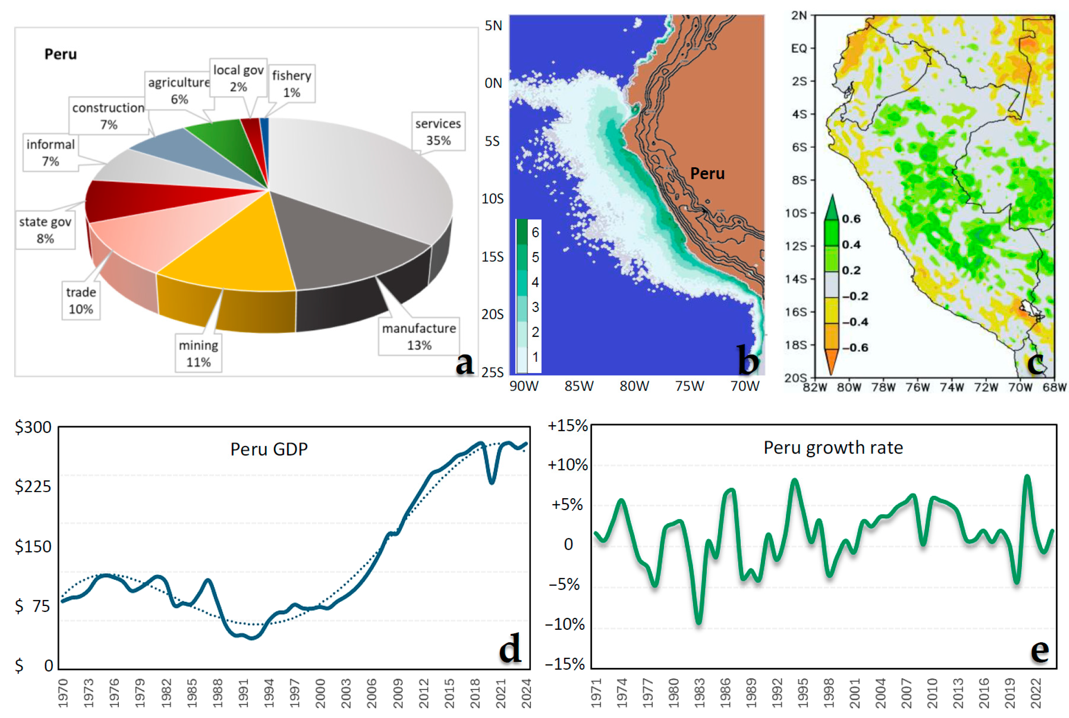
Figure 1. (a) Pie chart of sectoral contributions to the Peru GDP [3], (b) Satellite phytoplankton fluorescence (Sr−1) and Andes topography, (c) Correlation of Jan–Mar SOI with satellite vegetation color, green = productive during La Niña and unproductive during El Niño, country boundaries are included. (d) Raw annual gross domestic product (Billions US $) and (dashed) polynomial trend, (e) year-on-year change in GDP per capita inflation-adjusted.
Climate 13 00216 g001
Figure 2. Point-to-field correlation of growth rate onto Jan-Mar: (a) SST and (b) sea level air pressure (shaded at 0.2 interval), (c) temporal lag-correlation of SOI and Nino3 vs. Peru growth rate 1971–2024, with growth following and +/− quintiles (green); R > |0.26| is significant at 95% confidence (dashed).
Climate 13 00216 g002
Figure 3. Composite analysis of high minus low GDP years: (a) surface wind (vectors), (b) rainfall (mm), (c) ocean currents (vectors) and sea temperature (°C) in depth section averaged 10° S–7° N latitude; all represent Jan-Mar differences. (d) Dates employed and GDP change (%). Note that neutral outcomes are unshaded or have small vectors.
Climate 13 00216 g003
Figure 4. Composite analysis of high minus low GDP years, as height sections: (a) zonal circulation (vectors) and topography averaged 10° S–7° N, (b) meridional circulation (vectors) and zonal wind (contour), and (c) specific humidity (g/kg) and air temperature (°C, contour) averaged 70° W–85° W; all represent Jan–Mar differences. Note that neutral outcomes are unshaded or have small vectors.
Climate 13 00216 g004
Figure 5. Composite analysis of high minus low GDP years: (a) 500 hPa wind (vectors), (b) satellite net OLR (W/m2, blue = cloudy), (c) sea surface temperature (°C); all represent Jan-Mar differences. Note that neutral outcomes are unshaded or have small vectors.
Climate 13 00216 g005
Figure 6. (a) Multi-variate regression of the annual Peru GDP growth rate from Jan-Mar predictors and (b) scatterplot comparing prediction vs. observed and its (dashed) linear regression.
Climate 13 00216 g006
Disclaimer/Publisher’s Note: The statements, opinions and data contained in all publications are solely those of the individual author(s) and contributor(s) and not of MDPI and/or the editor(s). MDPI and/or the editor(s) disclaim responsibility for any injury to people or property resulting from any ideas, methods, instructions or products referred to in the content.