Benova and Cenova Models in the Homogenization of Climatic Time Series

Abstract

For the correct evaluation of climate trends and climate variability, it is important to remove non-climatic biases from the observed data. Such biases, referred to as inhomogeneities, occur for station relocations or changes in the instrumentation or instrument installation, among other reasons. Most inhomogeneities are related to a sudden change (break) in the technical conditions of the climate observations. In long time series (>30 years), usually multiple breaks occur, and their joint impact on the long-term trends and variability is more important than their individual evaluation. Benova is the optimal method for the joint calculation of correction terms for removing inhomogeneity biases. Cenova is a modified, imperfect version of Benova, which, however, can also be used in discontinuous time series. In the homogenization of section means, the use of Benova should be preferred, while in homogenizing probability distribution, only Cenova can be applied. This study presents the Benova and Cenova methods, discusses their main properties and compares their efficiencies using the benchmark dataset of the Spanish MULTITEST project (2015–2017), which is the largest existing dataset of this kind so far. The root mean square error (RMSE) of the annual means and the mean absolute trend bias were calculated for the Benova and Cenova results. When the signal-to-noise ratio (SNR) is high, the errors in the Cenova results are higher, from 14% to 24%, while when the SNR is low, or concerted inhomogeneities in several time series occur, the advantage of Benova over Cenova might disappear.

1. Introduction

The understanding, adaptation to and forecasting of climatic processes need the quantitative knowledge of the near past trends and variability. Regarding the earth surface climate observations, the Global Climate Observing System of the World Meteorological Organization classifies air temperature, precipitation amount, water vapor, wind speed, wind direction, atmospheric pressure and surface radiation budget to be essential climate variables (ECVs) [1]. Over the past 100–150 years, weather events and climate parameters have been regularly observed and recorded at observing stations operated by national meteorological services. As a result, a large volume of generally high-quality data is available for analyzing recent climate change and variability. However, in the evaluation of the global-, regional- and small-scale climate variability, one faces three main problems: (i) The density of observations has gradually increased, and the data amount from the early periods (say, before the middle of the 20th century) is notably smaller, and the related data quality problems are more frequent than for the data of the modern era; (ii) the density of observation is still highly uneven, it is still low for some ECVs and generally low in poor countries [2]; (iii) even when long records of observations of sufficient spatial density are available, the usability of the time series is compromised for technical changes occurred during the observations. This means that a part of the seeming trends and variability are not caused by the climate but by factors like station relocation, changes in the instrumentation, instrument installation, timing or technical execution of the observations, etc. [3,4,5,6]. The homogenization of climatic time series deals with the separation of technical or environmental effects (referred to as station effects) from the true climate signal, and this is the topic of the present study.

Most inhomogeneities are linked to a technical change at a specific date, e.g., a station relocation or instrument change causes a sudden change, referred to as break, in the station effect. Not every change in the station effect constitutes a break, since attrition or environmental changes may be gradual. However, time series of observed climatic data are generally modeled with station effects comprising only break-type changes because the use of more complex models [7,8,9] has not yielded improved efficiency [10,11].

Generally, an observed climatic value (x) is the sum of the climate signal (u), station effect (v) and noise (ε); the latter is caused by the temporal variation of the spatial distribution of climate parameters (can be referred to as weather effect) and non-systematic observation errors. Note that when a time series is homogeneous, v is constant, but even in that case, its value usually differs from zero for the local deviation of the climate from the regional mean climate. Denoting the vectors of the time series of n observed data with bold capital letters, this can be formulated by Equation (1):

$$\mathbf{X}=\mathbf{U}+\mathbf{V}+\mathsf{\epsilon } (\mathbf{X}=x_1,x_2,\dots x_i\dots x_n)$$

(1)

The noise has zero expected value, and thus, it is often omitted from the formulas. Generally, a time series contains K breaks (0 ≤ K < n), which divide X to K + 1 homogeneous sub-periods (HSPs). Denoting the timing of the breaks with j₁, j₂, …, j_k, … j_K, X can also be characterized by Equation (2):

$$\mathbf{X}=u_1+v_1,\dots u_{jk}+v_k,u_{jk+1}+v_{k+1},\dots u_n+v_{K+1}$$

(2)

Equation (2) suggests that the station effect is constant within an HSP, but seasonal variations and/or variations according to the percentiles of probability distribution (PDF) of x may occur in v, even within an HSP. These facts indicate that the homogenization of climatic time series is a complex task, and indeed, it has various aspects and subtasks [12,13,14,15,16,17,18,19,20]. Generally, the homogenization of the section means is the most important, both because it improves the accuracy of trend calculations, and the signal-to-noise ratio (SNR) provides the highest potential improvement for the accuracy of section means. Notwithstanding, this study analyzes some methodological questions of the homogenization of PDF. Note that the station effect is multiplicative for some climatic variables, of which the precipitation amount is the most important. However, such time series are subjected to function transformation before homogenization, and in this way Equations (1) and (2) correctly characterize the role of inhomogeneities for any climate variable. In practice, the observed values x are known, while u and v have only estimated values, even when all the break positions are known; the precise values of u and v also depend on the noise and the spatial differences of the climate.

Turning back to the principal problem of homogenization, which is the separation of station effect from the true climate variability, it has two principal tools: documented information (metadata) about the technical changes and statistical homogenization. Statistical homogenization is almost always based on the comparison of time series originating from the same climatic region (relative homogenization), since any distinction between climatic changes and inhomogeneities is uncertain without the mentioned comparisons. A special case is when metadata contain full information about the date and size of a break caused by a technical change, which is possible when parallel measurements were performed with old and newly introduced technical conditions [21,22,23,24,25]. For the quantification of most inhomogeneities, data of parallel observations are not available, and even the dates of the breaks are often unknown. Tests with benchmark datasets show that statistical homogenization generally improves the data accuracy when the station density provides sufficient SNR for performing relative homogenization [26,27,28,29,30]. Beyond low station density, possible occurrences of synchronous or semi-synchronous inhomogeneities in several time series of a given climatic region (they may be referred to as clustered inhomogeneities or clustered break systems) threaten the success of statistical homogenization the most. A principle of relative homogenization is that the climate signal is presumed to be valid for a region, while inhomogeneities are station-specific. However, technical changes are sometimes introduced for networks of observing stations within relatively short periods. In such cases, the availability of correct documentation may be crucial. Finally, the efficiency of homogenization also depends on the applied statistical methods.

Statistical homogenization has a long history [13]. Early methods [31,32,33,34] focused mostly on the accurate detection of individual breaks, while the introduction of the concept of multiple break homogenization [35,36] in the 1990s started to change the paradigm of effective homogenization. The new paradigm does not negate the importance of individual breaks (particularly those of large magnitudes) but focuses more on the combined effect of multiple breaks on the biases of trends and long-term variability. The reasoning of this change is that long time series generally contain multiple breaks [4,26,37], and a notable ratio of the breaks are too small for their precise detection [26,37,38,39,40]. Note that the described paradigm change still has not been finished, and in practical homogenization the multiple break approach is not yet generally used in the calculation of adjustment terms and the homogenization of PDF.

The aims of the present study are (i) enhancing the importance of the Benova method [36,41] for the joint calculation of adjustment terms at the bias removal phase of homogenization procedures; (ii) enhancing the importance of the multiple break approach in the homogenization of PDF; and (iii) testing the Cenova model [42], which is a modified version of Benova. Cenova is an imperfect version of Benova, but it is arguably useful in the homogenization of PDF [42], since Benova cannot be applied in PDF homogenization. The testing of the differences between Benova efficiency and Cenova efficiency is necessary to obtain quantitative knowledge about the suitability and possible drawbacks of using the Cenova model for tasks where Benova is not applicable.

In Section 2, the Benova and Cenova models are presented, and their usability is briefly discussed. In Section 3, the accuracies of Benova and Cenova models are compared by embedding them into the ACMANT homogenization method [43,44] and using the benchmark dataset of the Spanish MULTITEST project [30]. Finally, in Section 4 and Section 5, the discussion and conclusions are presented, respectively.

2. Methods

This section is divided into five sub-sections. Section 2.1 presents some general notes about the use of statistical models in climatology. In Section 2.2 and Section 2.3, Benova and Cenova are presented, respectively. In Section 2.4, the estimation of the network mean climatic trends is discussed because the removal of such trends is indispensable before using Cenova. In Section 2.5, the background software ACMANTv5.3 is briefly presented.

2.1. Use of Statistical Models in Climatology

Three main modes of using statistical models are discussed here: (i) The statistical model perfectly describes the climatological task; (ii) the selected statistical model fairly describes the climatological tasks, but the model conditions are not fully completed; (iii) the usefulness of the selected statistical model can only empirically be proven. An example for (i) is the observation of wind speed by recording the route length of the cups of a cup-anemometer within known time spans, since the wind speed can perfectly be calculated from the ratio of route length to time for speeds occurring in climatology. An example for (ii) is the calculation of the seasonal variation of temperature from a sinus-shaped annual cycle. The usability of the model can be examined by the closeness of the observed annual cycle to the used harmonic cycle. An example for (iii) is that the daily mean temperature can be estimated from averaging the daily minimum temperature and daily maximum temperature (and often no more accurate method is possible for the periods of manned observations). The adequacy of this approach has only empirical proof.

The results of relative homogenization are not perfectly accurate for the noise of the time series, among other reasons [12,13,14]. However, Benova can be considered a type (i) model within the family of relative homogenization procedures, since Benova does not contain other conditions or error sources than those of the relative homogenization model itself. This aspect of Benova was analyzed in detail in [40]. In contrast with Benova, Cenova is a type (iii) model, and its usability needs experimental justification.

2.2. Benova Model

Benova is the equation system of the relative homogenization model described for a network of climatic region whose N time series are homogenized together. It consists of the averages for each HSP of each time series (s) (Equation (3)) and the regional mean climate signals for each time point (i) of the time series (Equation (4)):

$${\displaystyle \frac{1}{j_{s,k+1}-j_{s,k}}}{\sum }_{i=j_{s,k}+1}^{j_{s,k+1}}\widehat{u_i}+\widehat{v_{s,k}}=\overline{{\mathit{x}}_{\mathit{s},\mathit{k}}}$$

(3)

$$\widehat{u_i}+{\displaystyle \frac{1}{N}}{\sum }_{s=1}^N\widehat{v_{s,k\left(i\right)}}={\displaystyle \frac{1}{N}}{\sum }_{s=1}^N{x}_{s,i}$$

(4)

In Equations (3) and (4), upper stroke denotes the arithmetical average, and cup over a letter indicates estimated value. Once the number of breaks and their positions in the time series have been estimated, Benova can be used to estimate the shift sizes between consecutive HSPs. The method was first applied by Caussinus and Mestre [36], who called it “ANOVA”. The name has been changed to Benova to prevent possible confusions (the name ANOVA is widely used for analysis of variance). The properties of Benova were examined by [41,45,46]. The method is widely applicable, and its results are optimal both theoretically and according to test experiments. Note that the absolute values of the station effect cannot be calculated by the equation system, only its temporal variations [41,46].

In a developed version of Benova, referred to as weighted Benova model, spatial differences of the climate are considered by weighting the time series. The introduction of weights (w) transforms Equation (4) to Equation (5):

$${\sum }_{s=1}^N{w}_s\widehat{u_{s,i}}+{\sum }_{s=1}^N{w}_s\widehat{v_{s,k\left(i\right)}}={\sum }_{s=1}^N{w_{s}x}_{s,i}$$

(5)

The weights are considered from the point of view of a given candidate series (for which w = 1) while 0 < w < 1 for the other time series of the network. The theoretically optimal weights are provided by ordinary kriging [47]. Test experiments (not shown) indicate small differences according to weightings, since the accuracy of Benova depends most on the suitability of the break detection results.

Note that metadata dates can be used in Benova in the same way as statistically detected break dates.

2.3. Cenova Model and the Homogenization of PDF

Cenova is a recently constructed, modified version of the parent Benova model [42]. Its creation was motivated by a development in the homogenization of probability distribution (PDF).

The homogenization of PDF is a relatively new line in the development of climatic datasets, i.e., the first study was published in 2006 [48]. The method is called quantile matching (QM), and its core is that the PDF is divided to sections of predetermined percentile ranges both in the candidate series and its reference series. This division is performed independently on the two sides of any break, then the differences between the candidate series and reference series are compared between the two sides of the break for each percentile range. These differences provide the first break-size estimations, which are refined by smoothing between the adjacent percentile ranges. Quantile matching has some later versions [38,49,50,51], and it has become a rather frequently applied method [52,53,54,55,56]. In some versions, regression analysis partly or fully substitutes the use of percentile ranges. In all QM versions, limited ranges of the time series are used on both sides of a break, and neighbor series with break(s) close to the examined break of the candidate series are excluded. This means that QM examines individually each break, disregarding the combined effects of multiple inhomogeneities, and the limitations in the use of neighbor series or their sections cause information loss. The few available method comparison test results [27,28,49] confirm that QM produces notably weaker results than other homogenization approaches.

The principal aims of the recent development of the HPDTS method (Homogenization of Probability Distribution for Time Series) were to use all data of an appropriately constructed network of time series and calculate quantile-dependent inhomogeneity biases by an equation system similar to Benova. The solution is provided by the Cenova model, detailed below. The full description of the HPDTS method and a wider discussion about the existing options for PDF homogenization are presented in [42].

The Benova model can only be applied to temporally continuous data fields. When the data belonging to a specific percentile range are considered, they represent only 5–10% of the parent time series. Therefore, in the Cenova model, the time series of the daily data of a given percentile range are filled with the arithmetical averages (x’) for determined periods similar to HSPs and denoted with HSP*s. In the candidate series, the HSP*s are identical to the HSPs, while in the neighbor series, the break dates of the candidate series are added to the own breaks of the series in the construction of HSP*s. This modification does not cause an effective change in Equation (3) but does impact the accuracy of Equations (4) and (5). The equations for individual time points (usually days in PDF homogenization) can be summed and/or averaged without any impact on the break size estimations when no break occurs in any of the time series of the network within the period of summing or averaging. When the averaging is extended over different HSPs of series (s), this causes error ∆x(s,i) = x’ − x via the imperfect consideration of the station effect first in X_s, and it propagates to the other variables due to the interdependence among the variables of the equation system. The impact of this type of error is high when the climate has strong trends or low-frequency variability. This problem is illustrated by the simple example below.

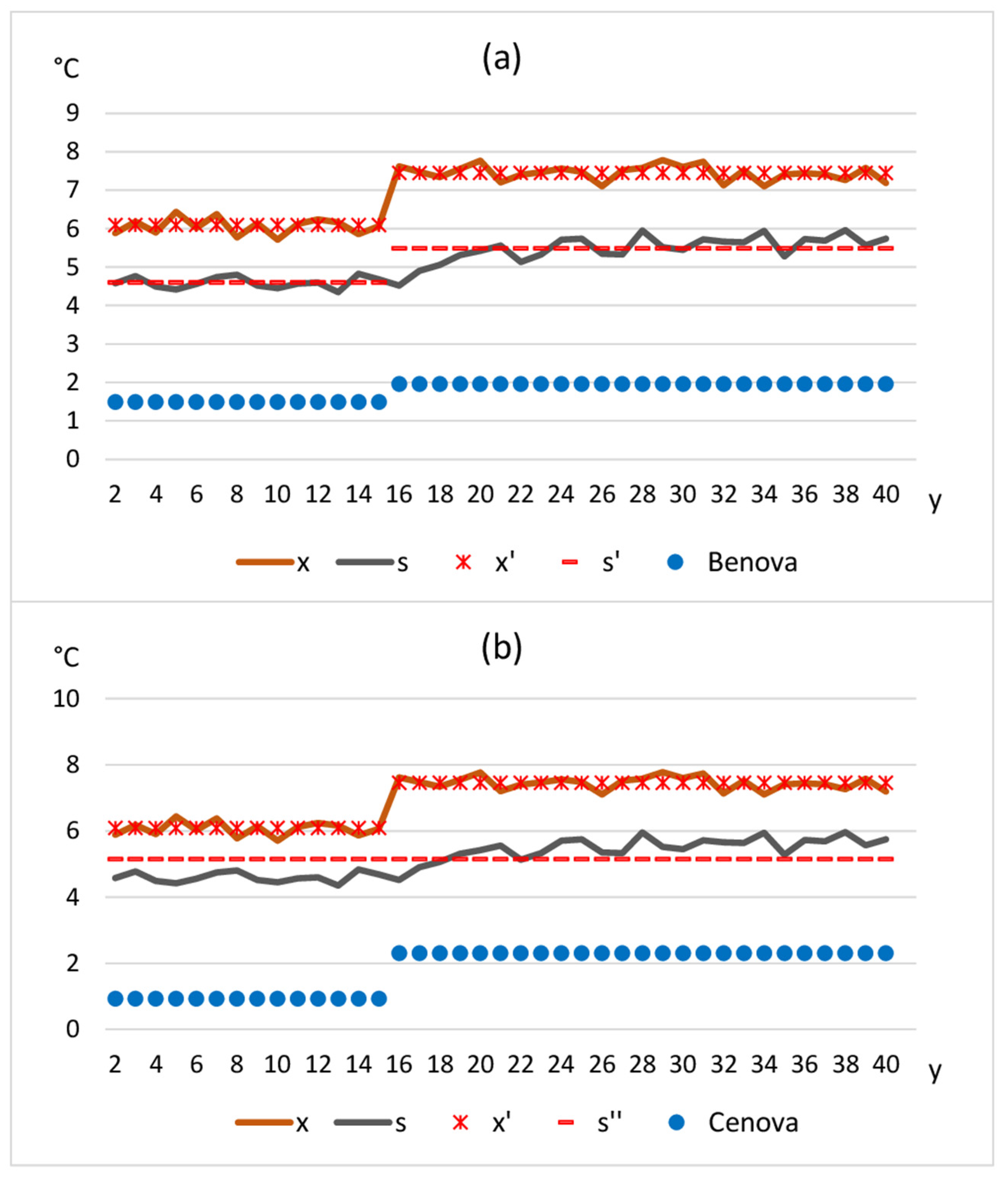
Two 40-year-long synthetic annual temperature time series, X and S, were created. S is supposed to be the composite reference series of X. Both X and S comprise the common climate signal, a station effect, and a Gaussian white noise with 1 °C standard deviation. The climate signal is a linear trend with 0.05 °C/year increase. S is homogeneous, while X has a break, with +1.0 °C shift 15 years after the beginning of the time series. When only one break occurs in a network of time series, the Benova results are identical with the differences between the HSP means of the relative time series where relative time series is defined as the difference between the candidate series (X) and its reference series (also see Section 6.2 of [14]). Figure 1 illustrates the break-size estimation result of Benova, which fairly approaches the true break size. However, when the averaging for HSP*s is performed according to the Cenova procedure, the climatic trend disappears from series S, causing a large estimation error (Figure 1b).

From Figure 1, one could conclude that shorter HSP* sections should be used in Cenova. In Section 4.3, this issue is discussed, highlighting that such shortening of HSP* sections does not generally create good solutions; therefore, the climatic trends must be removed from all series of the studied network before using Cenova.

2.4. Removal of Network Mean Trend Before Applying Cenova

The aim is to minimize the overall error caused by the accumulated impact of ∆x deviations, and one can take the benefit that the climate signal is neutral to the results of Benova and Cenova equation systems, except for deviations ∆x and their accumulated impact. The latter is the lowest when the network mean climatic trend is zero; therefore, the estimated network mean climatic trend is removed before the use of Cenova.

When Cenova was applied in the recent study of HPDTS [42], the section means had already been homogenized by previous procedures; thus, the network mean trend was presumed to be free of inhomogeneity bias. However, there are two problems with this approach: (i) The removal of network mean trend bias might fail for the presence of clustered breaks or low SNR; (ii) the network mean trend bias might notably differ for the extreme tails of the PDF in comparison to that of the means. Regarding the Cenova application in HPDTS, a new solution is proposed here, which takes into consideration possible errors related to point (ii). According to this, the adjustment terms are calculated by a Benova model of annual resolution for each percentile range. In the execution of this annual homogenization, each break timing is moved to the nearest end of year day (31 December). Breaks between January and June are pushed backwards, while those between July and December are pushed forward. The sorting of daily observed values (x) to percentile ranges is performed separately in each year, and then the annual averages are calculated for each percentile range. The time series constructed in this way are continuous, and the network mean climatic trends can be calculated for them by Benova. Then, the homogenized network mean low-frequency changes are estimated by a low-pass filter for each examined percentile range, and this climate signal is removed before applying Cenova.

Regarding the tests in Section 3, only section means are homogenized, since comparative tests for Benova and Cenova can only be performed in homogenization tasks for which both methods can be applied. In this case, the results of the second homogenization cycle of ACMANT can be directly applied to remove the network mean low-frequency changes.

2.5. ACMANTv5.3

ACMANT (Applied Caussian–Mestre Algorithm for the homogenization of Networks of climatic Time series) is a relative homogenization method for removing non-climatic biases from daily and monthly time series. Section mean values can be homogenized with or without the consideration of the seasonal variation of inhomogeneity biases. The method can be applied to the homogenization of temperature, precipitation amount, relative humidity, wind speed, wind gust, sunshine duration, radiation and atmospheric pressure. The inhomogeneous time series are modeled by homogeneous sections between consecutive breaks. The homogenization procedure contains three main homogenization cycles, and beyond them, preparatory steps before the first cycle and final operations, including refinements of the homogenization results of the third homogenization cycle, are also parts of the method. ACMANTv5.3 can homogenize up to 5000 time series in one run, and it solves the edition of networks of climatically comparable time series [57]. In all parts of the method, the evaluation of the combined effects of multiple breaks on the long-term trends and variability is prioritized. The break detection is performed with the maximum likelihood method proposed by [36], although with some modification in the parameterization of the Caussinus–Lyazrhi criterion [58] and with the inclusion of bivariate detection for selected homogenization tasks [43,59]. The principal way of time series comparison is the use of composite reference series [60], although the combined time series comparison [44] is performed in the first homogenization cycle, which includes the automatized pairwise comparison method developed by [9]. The correction terms for removing inhomogeneities are calculated by Benova. ACMANT includes ensemble homogenization [19] for attenuating random effects on the homogenization results, and applies distinct procedures for the detection and correction of outlier values and those of the large, short-term (<5 months) inhomogeneity biases. The method infills the data gaps with spatial interpolation and can use metadata automatically [61] if the list of metadata dates is provided together with the input climatic data. In running ACMANTv5.3, users may change some default parameters of the method and may opt for automatic or interactive homogenization. In interactive homogenization, users may modify the automatically constructed networks and the list of the detected breaks of the first homogenization cycle.

3. Comparative Tests for Benova and Cenova

3.1. Test Data

In the selection of the test dataset, three main factors were considered:

(i)

The homogeneous data must be perfectly known; therefore, only synthetically developed data can be used;

(ii)

The closeness to the real climate data properties, the size of the dataset and the variety of homogenization problems should allow for obtaining reliable test results;

(iii)

Both the Benova and Cenova models can be applied.

The selected dataset is the openly available benchmark dataset of the MULTITEST project [62]. This benchmark consists of 12 subsets of synthetic monthly temperature time series, the total number of independently edited climatic networks is 1900, and each network contains 5 to 40 time series of 40 to 100 years in length. The benchmark has homogeneous and inhomogeneous parts. For six subsets, the homogeneous part is created synthetically, adding independent Gaussian noise to a base temperature series of a Spanish observing station (Valladolid, 41.7° N, 4.7° W). These subsets are denoted by Y1, Y2, … Y6. For the other six subsets, the homogeneous part is an adaptation of the dataset development of [27], and it mimics the temperature climate of some U.S. regions; they are denoted by U1, U2, … U6. Each subset includes at least 100 networks. The subsets differ in the spatial correlations between time series within a network and in the properties of the inserted inhomogeneities into the time series, among other details [29]. The results are presented in the body text for three groups of the subsets: they are the high-SNR group (Y1, Y2, Y4, and U2), low-SNR group (Y3, U1, U3, and U4) and group of subsets including clustered break systems (Y5 and Y6). The results for each individual subset are shown in Appendix A.

3.2. Execution of Tests

For testing Benova, the homogenization method of ACMANTv5.3 was run without any change, since this method calculates the correction terms with Benova. In testing Cenova, a modified algorithm of the ACMANT procedure was used. In this algorithm, the content of ACMANTv5.3 is kept unchanged up to the end of the second homogenization cycle of the procedure. Thereafter, the low-frequency variation of the climate for a network is estimated from the results of the second homogenization cycle, and that is removed from each time series. Then, Cenova is applied instead of Benova for the calculation of the correction terms for the annual means. No other change is applied in comparison to ACMANTv5.3.

3.3. Test Results

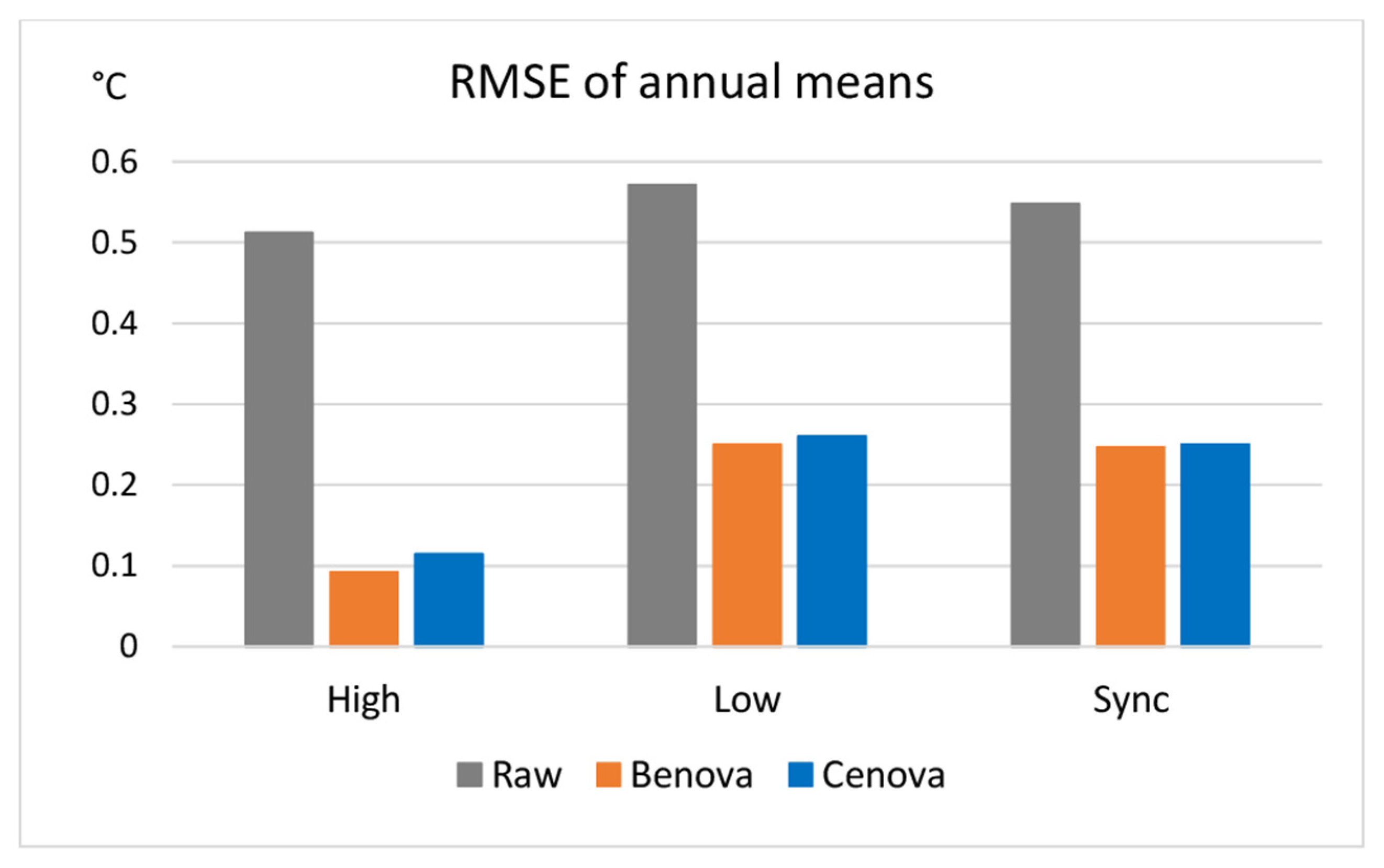
Three efficiency measures are applied for comparing the Benova and Cenova results: the root mean square error (RMSE) of annual means, the mean absolute trend bias for individual time series and the mean absolute network mean trend bias. The RMSE of monthly values is not examined here because Cenova was applied only for the corrections of the annual means. Figure 2 shows the results for the annual RMSE.

For high-SNR subsets, the lowest mean RMSE is achieved by using Benova, which confirms that Benova is more accurate than Cenova, although the difference between the results of Benova and Cenova is moderate, and a large part of the raw data errors are removed by either of the two examined methods. For the groups of low SNR and clustered breaks, the removal of raw data errors is much less successful than for the subsets of high SNR, and the differences between Benova and Cenova results are very small. The likely explanation for the relative lack of the advantage of using Benova for these groups of homogenization tasks is that the averaging of observed values within an HSP* of the Cenova method may favor the accuracy of homogenization results when the HSP* includes undetected breaks. This issue is discussed in Section 4.1.

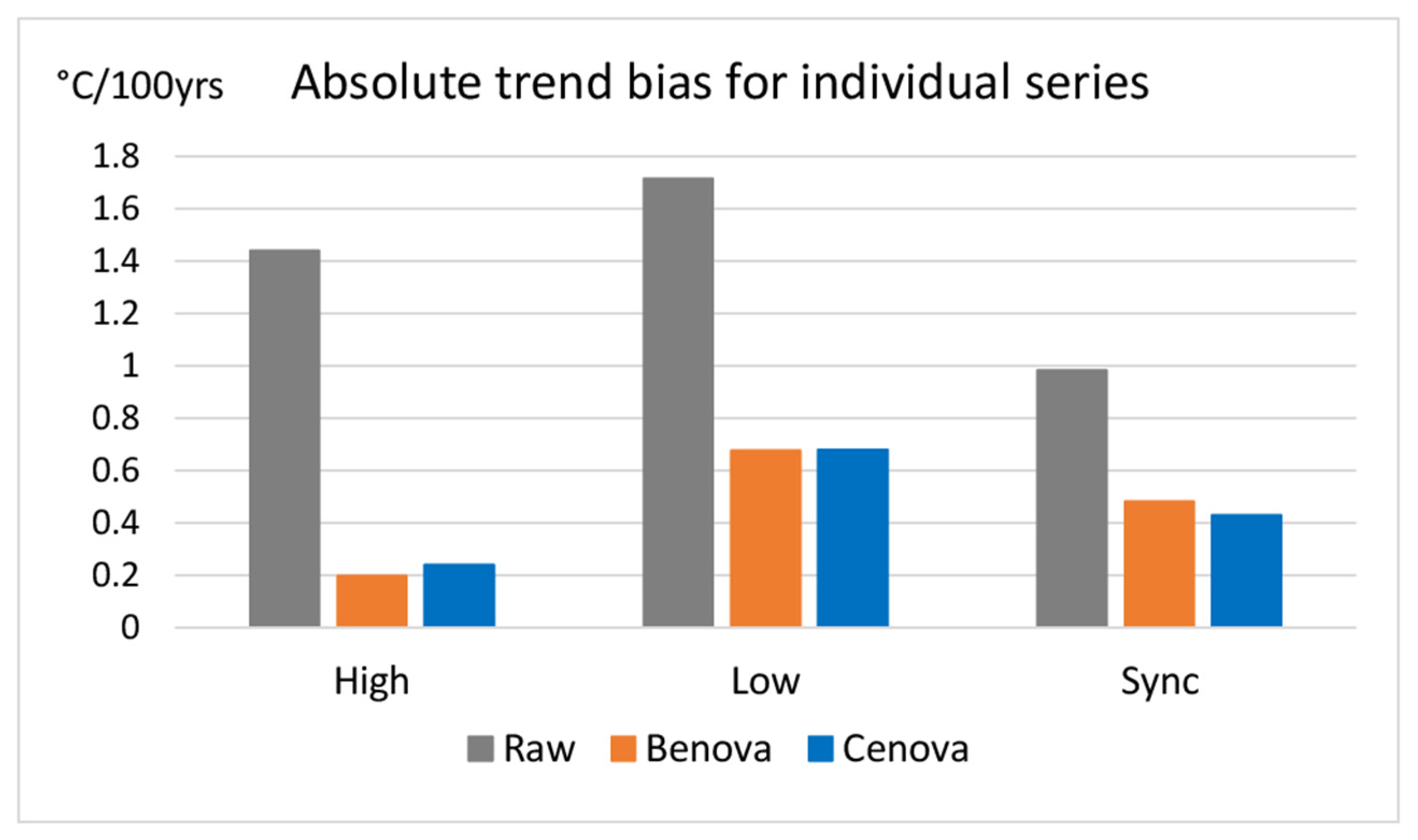
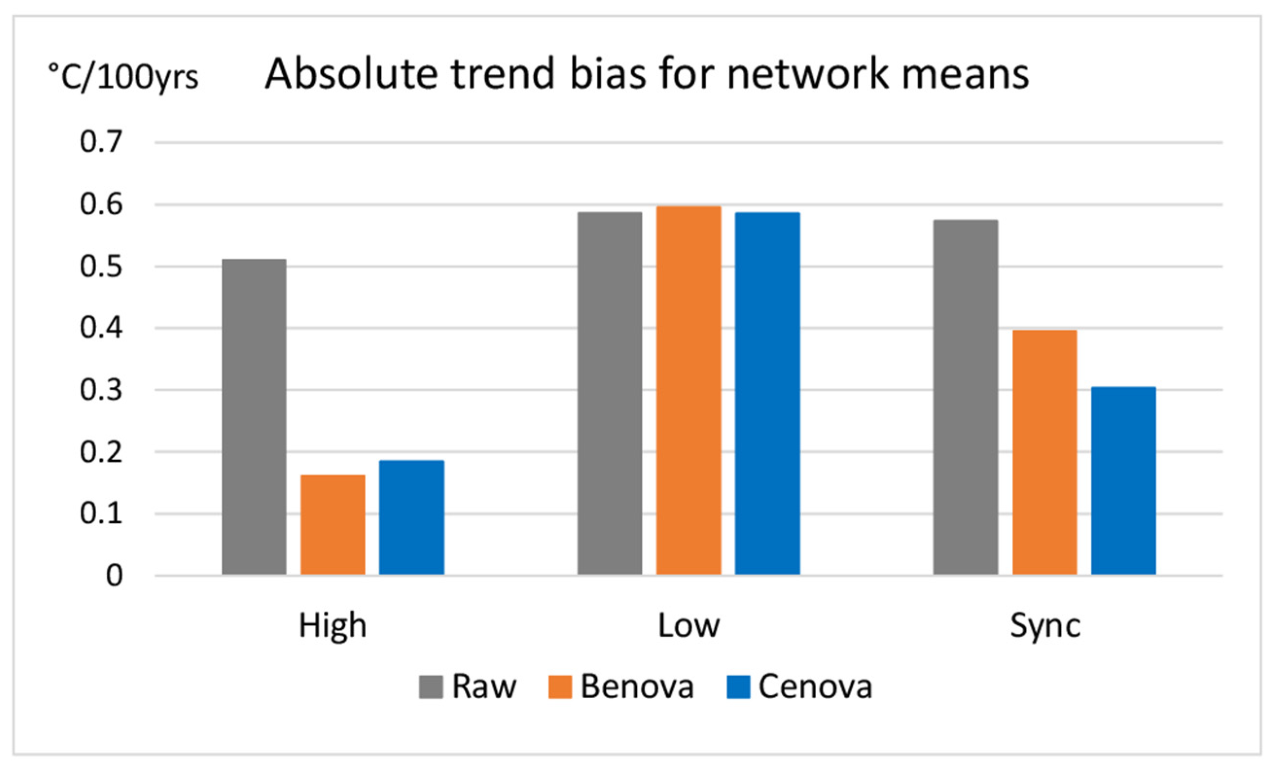
Figure 3 and Figure 4 show the mean absolute trend bias errors for individual time series and network means, respectively. The results of Figure 3 and Figure 4 show several similarities to the results shown in Figure 2, from which the most important feature is that a large portion of the raw data errors can be removed when the SNR is favorable, and in such cases, Benova shows a moderate but clear advantage over Cenova. When the SNR is low or clustered breaks occur, the removal of network mean trend bias is largely unsuccessful, while a notable part of the individual trend bias errors are still successfully removed. In cases of low SNR or the presence of clustered breaks, the use of Benova does not provide better trend bias removal than that of Cenova; moreover, for the examined subsets with clustered break systems, the trend bias removal for networks is notably more successful with Cenova than with Benova. The explanation is again the fact that averaging the observed values over an HSP* section is advantageous when the section includes undetected breaks.

Overall, the advantage of using the perfect model Benova has only been found for the group of high-SNR test datasets. In these cases, Cenova left larger residual errors of homogenization by 14% (for network mean trend bias) to 24% (for the RMSE of annual means) in comparison to the Benova results. While the differences in efficiency are notable in terms of ratios, they are less important in terms of the absolute values of the residual errors, since both Benova and Cenova removed a large part (60 to 85%) of the raw data errors for the high-SNR group.

4. Discussion

4.1. Impacts of Undetected Breaks and Network Mean Inhomogeneity Bias

If a neighbor series contains undetected breaks, averaging its values within the Cenova procedure may even improve the accuracy of the homogenization results. This impact is visible when the direction of a detected shift in the candidate series has the same sign as the undetected shift of the neighbor series and is the strongest when several shifts (partly detected, partly undetected) of different series have the same sign within a relatively short period, i.e., when clustered breaks occur. An example of the homogenization of synthetic time series including a clustered break system is shown in Figure 5.

In Figure 5, forty-year-long sections of time series are examined. X is the candidate series, and S is its composite reference series. A clustered break system between year 14 and year 19 impacts a significant part of the time series of the network (individual series are not shown, except for X). No other break than those of the clustered break system occurs in the study period. Both X and S contain Gaussian white noise with 0 mean and 1 °C standard deviation, and there are no other climate fluctuations. Series S contains a gradual increase of 1.0 °C from year 14 to year 20 for the impact of the clustered break system.

When X is homogenized with Benova, the undetected breaks of the neighbor series notably reduce the detected break size (Figure 5a). However, when Cenova is applied, the averaging of observed values within the shown HSP* acts as a pre-homogenization of the reference series (Figure 5b). The presented example with the correct detection of only one break position includes some simplifications, but it is still representative of realistic examples of the MULTITEST benchmark. During the MULTITEST project, nine versions of five fully automatic and openly available homogenization methods were tested (ACMANT, Climatol [63,64], MASH [35,65], PHA [9] and RHtests [66,67]). None of these methods could reduce the raw network mean trend bias error by more than 40% (21%) for the Y5 (Y6) subset.

The favorable results of Cenova in Figure 4 for networks including clustered breaks is an additional positive feature of the method, but it does not question the general advantage of Benova over Cenova. The found capacity of Cenova for the reduction of biases caused by clustered breaks may have limited direct benefits on the reduction of such biases for the following reasons: (i) The presence of clustered breaks with notable break sizes is not very frequent. (ii) Clustered breaks are mostly caused by planned technical changes in observing networks; therefore, their presence is often known from metadata. When metadata does not indicate occurrences of clustered breaks, the results of Benova are generally more accurate than the results of Cenova. (iii) If the presence of clustered breaks is known from metadata, more powerful methods than Cenova can be applied to reduce network mean trend bias errors: they are the use of observed data of stations unaffected by the clustered breaks and/or the use of reanalysis data [68].

4.2. Reliability of Test Results

A general limitation of using tests for assessing the efficiency of a given method is that real-world problems may differ from the test tasks. The large size of the MULTITEST benchmark and the variety of homogenization problems according to the differences of the 12 subsets make the test results generally convincing; note, however, that only temperature time series were used, and all of them mimic mid-latitude temperature climate. Earlier, the HPDTS procedure including Cenova was tested in some sections of another test dataset (INDECIS benchmark [28]), and those test results were also favorable [42]. Note that so far, the MULTITEST benchmark is the only openly available test dataset in which the number of independently generated networks for any given climate variable is higher than 15.

Another issue regarding the reliability of the test results is that Cenova is designed for the homogenization of the PDF of daily data, while the tests here were performed for the homogenization of section means of monthly series. In spite of this, there is only one detail in which the test procedure differs from the use of Cenova in HPDTS, and it is the calculation of the low-frequency variation of the climate signal. In the tests performed, this variation is calculated from the results of the second homogenization cycle of ACMANTv5.3. In HPDTS, it is proposed to be calculated using a model of annual resolution (see Section 2.4). Both the tested and proposed methods are effective when the SNR is favorable, while in the homogenization of low SNR and clustered break system problems, both the Benova-based and Cenova-based homogenizations have limited efficiencies in reconstructing the network mean climate signal.

In the presented tests, the efficiencies of the Benova and Cenova methods embedded into the ACMANT homogenization procedure were compared. Some doubts might come from the fact that Benova is used in the first two homogenization cycles of ACMANTv5.3 in both of the compared homogenization procedures. However, this issue impacts only the accuracy of the input data of the Cenova procedure, which are the timings of the detected breaks and the temporal variation of the climate signal. In the performed tests, Cenova was applied to the raw, non-homogenized data. In HPDTS, Cenova is applied to the data for which the section means of the annual values have been homogenized. Notwithstanding, the homogenization of the section means and that of the PDF are two independent dimensions, at least in the actual development of ACMANT, and thus the use of Benova in the pre-homogenization cycles of ACMANT does not impact the efficiency of the Cenova method when Cenova is applied.

4.3. Options for the Joint Calculation of Correction Terms for the Data of Discontinuous Time Series

The test results show that the use of Cenova is a relatively good option for the homogenization of networks of discontinuous time series; however, it is only one option. Here, further four options are briefly discussed, focusing on the problem of PDF homogenization. In the options presented in this section, Benova can be applied to the estimation of the correction terms, but some additional error sources occur.

(i)

Infilling data gaps before the homogenization of percentile ranges.

In PDF homogenization, the existence of this option is only theoretical, since the ratio of independent information would become very low (often only 10% or even lower). In addition, values from spatial interpolations would not represent the same percentile range as the selected data.

(ii)

Homogenization in the annual resolution, after the modification of the input data of PDF homogenization, in the way described in Section 2.4.

The actual proposal for PDF homogenization includes the use of this option but only for the estimation of the network mean low-frequency climate variation. If this method was used for correcting inhomogeneity biases in individual time series and in all time scales, the errors coming from shifting the break timings to the end of year date could be larger.

(iii)

Shortening the HSP* sections as long as none of such sections overlap break timings, not even when the break is in another time series than the HSP*.

Figure 1 suggests (Section 2.3) that the accuracy of Cenova could be improved by shortening the HSP*s. However, a problem with this option is that the number of days with observed values for a given percentile range decreases proportionally to the length of the HSP*. In the actual parameterization, the usual minimum length of an HSP* is 9 months, while it may be as short as 5 months in some special cases. Even these thresholds can be too low, since the number of days with observed values for a percentile range can be lower than 20, and thus, the accuracy of the estimations for HSP* means may be affected both by low sample size and autocorrelation.

(iv)

Dates without observed values can be skipped before using Benova.

While it is true, it can be applied only when the data gaps are synchronous, and this is not the case in HPDTS. An option for homogenizing PDF is that only the data of the candidate series are sorted according to quantiles, and in homogenizing a given percentile range, the values of the candidate series are compared to the synchronous data of the neighbor series. In this case, the dates without data in the candidate series can be skipped, and Benova can be applied. However, during the development of HPDTS, I found this option less promising than the actual solution; for instance, HSPs of neighbor series without data or with a very low number of data could occur.

Altogether, the use of the annual resolution for the estimation of the low-frequency climate variability and the use of Cenova for the other details of PDF homogenization is only one possible solution, but it seems to be a good solution.

4.4. When to Use Benova and Cenova

Benova and Cenova can be used for the separation of the temporal variations of a local variable from the temporal variations of a variable with similar effects on the time series of a network (referred to as global factor) when the local variations can be modeled by a step function in every time series. The extension of the step function model is possible [41], but such extensions are generally unnecessary in climatological applications. Generally, Benova provides the optimal solution, but for discontinuous data fields, only the Cenova method can be applied. Long records of climate observations often contain data gaps of varied lengths, since technical or economic problems, as well as political events, may affect the continuity of observations and data recording [69,70]. When data gaps can be infilled with spatial interpolations, it is likely better to use spatial interpolation and Benova than applying Cenova, although this issue may need further examination. Before using Cenova, the estimated low-frequency variation of the global factor must be removed.

Table 1. Required conditions for using Benova or Cenova. Notes: ¹ The correlation threshold may differ from the one shown; ² when spatial correlations are not calculated, the unweighted versions of Benova and Cenova (Equations (3) and (4)) can still be applied; ³ Benova could also be applied to trend inhomogeneities but that would need other formulas [41].

	Benova	Cenova
Number of time series	3≤	3≤
Spatial correlations 1,2	0.4≤	0.4≤
Form of inhomogeneities 3	Breaks	Breaks
Low-frequency climate variation	Any	Reduced
Continuity of time series	Required	Not required

presents the required conditions for using Benova or Cenova.

In the homogenization of the section means of climatic variables, the use of those homogenization methods should be preferred, which include Benova. Such methods are PRODIGE [36], ACMANT, Bart [71,72], HOMER [73] and AHOPS [74]. For the homogenization of PDF, the joint calculation of correction terms is also advantageous; therefore, the proposals of [42] and this study should be considered.

Naturally, the efficiency of a homogenization method also depends on other factors than the method of the calculation of correction terms. In a recent review paper about good practices in time series homogenization [17], the authors put six factors into focus: seasonality, autocorrelation, time series comparison, climatic trends, the shape of the PDF and the approach to the multiple-break problem. All these factors are truly important, but I believe that their effective treatment, “good practices”, usually cannot be evaluated separately, since the joint effect of the steps of a given homogenization procedure determines its efficiency. Therefore, the widening of the testing of homogenization methods would be important.

Benova and Cenova are statistical methods, and they could also be used in other fields of science than climatology. Although the aims and conditions of the homogenization of climatic time series are rather specific, similar research tasks might occur in other kinds of investigations. For instance, global and local factors are both present in economic time series [75], and their temporal variations can often be characterized by multiple breaks [76,77].

5. Conclusions

The efficiencies of Benova and Cenova methods for the removal of inhomogeneity biases from climatic time series were examined using the large-size, synthetic monthly temperature dataset of the MULTITEST benchmark. The tests were performed by embedding Benova or Cenova into the ACMANTv5.3 homogenization procedure, and the reductions in annual RMSE, absolute trend bias for individual time series and absolute network mean trend bias were examined. The main conclusions are as follows:

• When the signal-to-noise ratio (SNR) is favorable, ACMANT removes the major part of the raw data errors. The results produced by using Benova are the most accurate, but the residual errors after homogenization are not much larger, even when Cenova is applied instead of Benova.
• When the SNR is low, or the time series are affected by synchronous or semi-synchronous inhomogeneities (clustered breaks), the efficiency of ACMANT is much lower than for high-SNR tasks, and the differences between the Benova results and Cenova results are generally very small.
• Low SNR and clustered break problems mostly affect the removal of network mean trend biases. When clustered breaks occur, Cenova tends to provide better results in trend bias removal, particularly in the removal of network mean trends.
• The use of Benova should be prioritized over Cenova when the conditions allow for choosing between them, despite the fact that occasionally Cenova could produce the best results.
• For the homogenization of probability distribution (PDF), Cenova can safely be applied, once the low-frequency variation of the estimated climate signal has been removed from each time series.

Overall, the research results prove that the data accuracy of climatic datasets could be improved by the wider practical application of Benova and Cenova methods. The present article is a part of a project supported by the Catalan Meteorological Service. The principal aim of the project is the creation of ACMANTv6, which will be released in the last quarter of 2025. In ACMANTv6, Benova will be used in the homogenization of annual and seasonal means, while Cenova will be used in the homogenization of probability distribution.

References

1. Bojinski, S.; Verstraete, M.; Peterson, T.C.; Richter, C.; Simmons, A.; Zemp, M. The concept of essential climate variables in support of climate research, applications, and policy. Bull. Amer. Met. Soc. 2014, 95, 1431–1443. [Google Scholar] [CrossRef]
2. McKinnon, K.; National Center for Atmospheric Research Staff (Eds.) The Climate Data Guide: GHCN-D: Global Historical Climatology Network Daily Temperatures. Available online: https://climatedataguide.ucar.edu/climate-data/ghcn-d-global-historical-climatology-network-daily-temperatures (accessed on 5 June 2025).
3. Aguilar, E.; Auer, I.; Brunet, M.; Peterson, T.C.; Wieringa, J. Guidelines on Climate Metadata and Homogenization; WCDMP-53, WMO-TD 1186; World Meteorological Organization: Geneva, Switzerland, 2003. [Google Scholar]
4. Auer, I.; Böhm, R.; Jurkovic, A.; Orlik, A.; Potzmann, R.; Schöner, W.; Ungersböck, M.; Brunetti, M.; Nanni, T.; Maugeri, M.; et al. A new instrumental precipitation dataset for the Greater Alpine Region for the period 1800–2002. Int. J. Climatol. 2005, 25, 139–166. [Google Scholar] [CrossRef]
5. Prohom, M.; Barriendos, M.; Sanchez-Lorenzo, A. Reconstruction and homogenization of the longest instrumental precipi-tation series in the Iberian Peninsula (Barcelona, 1786–2014). Int. J. Climatol. 2016, 36, 3072–3087. [Google Scholar] [CrossRef]
6. Camuffo, D.; della Valle, A.; Becherini, F. Instrumental and observational problems of the earliest temperature records in Italy: A methodology for data recovery and correction. Climate 2023, 11, 178. [Google Scholar] [CrossRef]
7. Alexandersson, H.; Moberg, A. Homogenization of Swedish temperature data. Part I: Homogeneity test for linear trends. Int. J. Climatol. 1997, 17, 25–34. [Google Scholar] [CrossRef]
8. Vincent, L.A. A technique for the identification of inhomogeneities in Canadian temperature series. J. Clim. 1998, 11, 1094–1104. [Google Scholar] [CrossRef]
9. Menne, M.J.; Williams Jr, C.N. Homogenization of temperature series via pairwise comparisons. J. Clim. 2009, 22, 1700–1717. [Google Scholar] [CrossRef]
10. Domonkos, P. Efficiency evaluation for detecting inhomogeneities by objective homogenisation methods. Theor. Appl. Climatol. 2011, 105, 455–467. [Google Scholar] [CrossRef]
11. Williams, C.N.; Menne, M.J.; Thorne, P. Benchmarking the performance of pairwise homogenization of surface temperatures in the United States. J. Geophys. Res. 2012, 117, D05116. [Google Scholar] [CrossRef]
12. Lindau, R.; Venema, V.K.C. The joint influence of break and noise variance on the break detection capability in time series homogenization. Adv. Stat. Clim. Meteorol. Oceanogr. 2018, 4, 1–18. [Google Scholar] [CrossRef]
13. Venema, V.; Trewin, B.; Wang, X.L.; Szentimrey, T.; Lakatos, M.; Aguilar, E.; Auer, I.; Guijarro, J.; Menne, M.; Oria, C.; et al. Guidelines on Homogenization; WMO-No. 1245; World Meteorological Organization: Geneva, Switzerland, 2020. [Google Scholar]
14. Domonkos, P.; Tóth, R.; Nyitrai, L. Climate Observations: Data Quality Control and Time Series Homogenization; Elsevier: Amsterdam, The Netherlands, 2022; 302p. [Google Scholar]
15. de Valk, C.; Brandsma, T. Homogenization of daily temperatures using covariates and statistical learning—The case of parallel measurements. Int. J. Climatol. 2023, 43, 7170–7182. [Google Scholar] [CrossRef]
16. Katata, G.; Connolly, R.; O’Neill, P. Evidence of urban blending in homogenized temperature records in Japan and in the United States: Implications for the reliability of global land surface air temperature data. J. Appl. Meteor. Climatol. 2023, 62, 1095–1114. [Google Scholar] [CrossRef]
17. Lund, R.B.; Beaulieu, C.; Killick, R.; Lu, Q.; Shi, X. Good practices and common pitfalls in climate time series changepoint techniques: A review. J. Clim. 2023, 36, 8041–8057. [Google Scholar] [CrossRef]
18. Chimani, B.; Bochníček, O.; Brunetti, M.; Ganekind, M.; Holec, J.; Izsák, B.; Lakatos, M.; Tadić, M.P.; Manara, V.; Maugeri, M.; et al. Revisiting HISTALP precipitation dataset. Int. J. Climatol. 2023, 43, 7381–7411. [Google Scholar] [CrossRef]
19. Domonkos, P. Relative homogenization of climatic time series. Atmosphere 2024, 15, 957. [Google Scholar] [CrossRef]
20. Lindau, R. Estimation of break and noise variance and the maximum distance of climate stations allowed in relative homogenisation of annual temperature anomalies. Int. J. Climatol. 2025, 45, e8724. [Google Scholar] [CrossRef]
21. Brunet, M.; Asin, J.; Sigró, J.; Bañon, M.; García, F.; Aguilar, E.; Palenzuela, J.E.; Peterson, T.C.; Jones, P. The minimization of the screen bias from ancient Western Mediterranean air temperature records: An exploratory statistical analysis. Int. J. Climatol. 2011, 31, 1879–1895. [Google Scholar] [CrossRef]
22. Vincent, L.A.; Wang, X.L.; Milewska, E.J.; Wan, H.; Yang, F.; Swail, V. A second generation of homogenized Canadian monthly surface air temperature for climate trend analysis. J. Geophys. Res. 2012, 117, D18110. [Google Scholar] [CrossRef]
23. Hannak, L.; Friedrich, K.; Imbery, F.; Kaspar, F. Analyzing the impact of automatization using parallel daily mean temperature series including breakpoint detection and homogenization. Int. J. Climatol. 2020, 40, 6544–6559. [Google Scholar] [CrossRef]
24. Ashcroft, L.; Trewin, B.; Benoy, M.; Ray, D.; Courtney, C. The world’s longest known parallel temperature dataset: A comparison between daily Glaisher and Stevenson screen temperature data at Adelaide, Australia, 1887–1947. Int. J. Climatol. 2022, 42, 2670–2687. [Google Scholar] [CrossRef]
25. Wallis, E.J.; Osborn, T.J.; Taylor, M.; Jones, P.D.; Joshi, M.; Hawkins, E. Quantifying exposure biases in early instrumental land surface air temperature observations. Int. J. Climatol. 2024, 44, 1611–1635. [Google Scholar] [CrossRef]
26. Venema, V.; Mestre, O.; Aguilar, E.; Auer, I.; Guijarro, J.A.; Domonkos, P.; Vertacnik, G.; Szentimrey, T.; Štěpánek, P.; Zahradníček, P.; et al. Benchmarking monthly homogenization algorithms. Clim. Past 2012, 8, 89–115. [Google Scholar] [CrossRef]
27. Killick, R.E. Benchmarking the Performance of Homogenisation Algorithms on Daily Temperature Data. Ph.D. Thesis, University of Exeter, Exeter, UK, 2016. [Google Scholar]
28. Guijarro, J.A. Recommended Homogenization Techniques Based on Benchmarking Results; WP-3 Report of INDECIS Project. 2019. Available online: http://www.indecis.eu/docs/Deliverables/Deliverable_3.2.b.pdf (accessed on 5 June 2025).
29. Domonkos, P.; Guijarro, J.A.; Venema, V.; Brunet, M.; Sigró, J. Efficiency of time series homogenization: Method comparison with 12 monthly temperature test datasets. J. Clim. 2021, 34, 2877–2891. [Google Scholar] [CrossRef]
30. Guijarro, J.A.; López, J.A.; Aguilar, E.; Domonkos, P.; Venema, V.K.C.; Sigró, J.; Brunet, M. Homogenization of monthly series of temperature and precipitation: Benchmarking results of the MULTITEST project. Int. J. Climatol. 2023, 43, 3994–4012. [Google Scholar] [CrossRef]
31. Wilcoxon, F. Individual comparisons by ranking methods. Biom. Bull. 1945, 1, 80–83. [Google Scholar] [CrossRef]
32. Maronna, R.; Yohai, V.J. A bivariate test for the detection of a systematic change in mean. J. Am. Stat. Assoc. 1978, 73, 640–645. [Google Scholar] [CrossRef]
33. Craddock, J.M. Methods of comparing annual rainfall records for climatic purposes. Weather 1979, 34, 332–346. [Google Scholar] [CrossRef]
34. Alexandersson, H. A homogeneity test applied to precipitationdata. J. Climatol. 1986, 6, 661–675. [Google Scholar] [CrossRef]
35. Szentimrey, T. Multiple Analysis of Series for Homogenization (MASH). In Second Seminar for Homogenization of Surface Climatological Data; Szalai, S., Szentimrey, T., Szinell, C., Eds.; WMO WCDMP-41; World Meteorological Organization: Geneva, Switzerland, 1999; pp. 27–46. [Google Scholar]
36. Caussinus, H.; Mestre, O. Detection and correction of artificial shifts in climate series. J. R. Stat. Soc. Ser. C Appl. Stat. 2004, 53, 405–425. [Google Scholar] [CrossRef]
37. Menne, M.J.; Williams, C.N.; Vose, R.S. The U.S. Historical Climatology Network Monthly Temperature Data, Version 2. Bull. Am. Meteor. Soc. 2009, 90, 993–1008. [Google Scholar] [CrossRef]
38. Štěpánek, P.; Zahradnicek, P.; Farda, A. Experiences with data quality control and homogenisation of daily records of various meteorological elements in the Czech Republic in the period 1961-2010. Időjárás 2013, 117, 123–141. [Google Scholar]
39. Lindau, R.; Venema, V.K.C. The uncertainty of break positions detected by homogenization algorithms in climate records. Int. J. Climatol. 2016, 36, 576–589. [Google Scholar] [CrossRef]
40. O’Neill, P.; Connolly, R.; Connolly, M.; Soon, W.; Chimani, B.; Crok, M.; de Vos, R.; Harde, H.; Kajaba, P.; Nojarov, P.; et al. Evaluation of the homogenization adjustments applied to European temperature records in the Global Historical Climatology Network Dataset. Atmosphere 2022, 13, 285. [Google Scholar] [CrossRef]
41. Domonkos, P.; Joelsson, L.M.T. ANOVA (Benova) correction in relative homogenization: Why it is indispensable. Int. J. Climatol. 2024, 44, 4515–4528. [Google Scholar] [CrossRef]
42. Domonkos, P. Homogenization of the probability distribution of climatic time series: A novel algorithm. Atmosphere 2025, 16, 616. [Google Scholar] [CrossRef]
43. Domonkos, P. ACMANTv4: Scientific Content and Operation of the Software, 2020; 71p. Available online: https://github.com/dpeterfree/ACMANT/blob/ACMANTv4.4/ACMANTv4_description.pdf (accessed on 5 June 2025).
44. Domonkos, P. Combination of using pairwise comparisons and composite reference series: A new approach in the homogenization of climatic time series with ACMANT. Atmosphere 2021, 12, 1134. [Google Scholar] [CrossRef]
45. Mamara, A.; Argiriou, A.A.; Anadranistakis, M. Detection and correction of inhomogeneities in Greek climate temperature series. Int. J. Climatol. 2014, 34, 3024–3043. [Google Scholar] [CrossRef]
46. Lindau, R.; Venema, V.K.C. On the reduction of trend errors by the ANOVA joint correction scheme used in homogenization of climate station records. Int. J. Climatol. 2018, 38, 5255–5271. [Google Scholar] [CrossRef]
47. Szentimrey, T. Methodological questions of series comparison. In Proceedings of the Sixth Seminar for Homogenization and Quality Control in Climatological Databases, Budapest, Hungary, 26–30 May 2008; Lakatos, M., Szentimrey, T., Bihari, Z., Szalai, S., Eds.; WMO WCDMP-76. World Meteorological Organization: Geneva, Switzerland, 2010; pp. 1–7. [Google Scholar]
48. Della-Marta, P.M.; Wanner, H. A method of homogenizing the extremes and mean of daily temperature measurements. J. Clim. 2006, 19, 4179–4197. [Google Scholar] [CrossRef]
49. Mestre, O.; Gruber, C.; Prieur, C.; Caussinus, H.; Jourdain, S. SPLIDHOM: A method for homogenization of daily temperature observations. J. Appl. Meteorol. Climatol. 2011, 50, 2343–2358. [Google Scholar] [CrossRef]
50. Squintu, A.A.; van der Schrier, G.; Brugnara, Y.; Klein Tank, A. Homogenization of daily temperature series in the European Climate Assessment & Dataset. Int. J. Climatol. 2019, 39, 1243–1261. [Google Scholar] [CrossRef]
51. Squintu, A.A.; van der Schrier, G.; Štěpánek, P.; Zahradníček, P.; Klein Tank, A. Comparison of homogenization methods for daily temperature series against an observation-based benchmark dataset. Theor. Appl. Climatol. 2020, 140, 285–301. [Google Scholar] [CrossRef]
52. Trewin, B.; Braganza, K.; Fawcett, R.; Grainger, S.; Jovanovic, B.; Jones, D.; Martin, D.; Smalley, R.; Webb, V. An updated long-term homogenized daily temperature data set for Australia. Geosci. Data J. 2020, 7, 149–169. [Google Scholar] [CrossRef]
53. Brugnara, Y.; McCarthy, M.P.; Willett, K.M.; Rayner, N.A. Homogenization of daily temperature and humidity series in the UK. Int. J. Climatol. 2023, 43, 1693–1709. [Google Scholar] [CrossRef]
54. Resch, G.; Koch, R.; Marty, C.; Chimani, B.; Begert, M.; Buchmann, M.; Aschauer, J.; Schöner, W. A quantile-based approach to improve homogenization of snow depth time series. Int. J. Climatol. 2023, 43, 157–173. [Google Scholar] [CrossRef]
55. Chen, J.; Hu, T.; Wang, J.; Yan, Z.; Li, Z. A method for homogenization of complex daily mean temperature data: Application at Beijing Observatory (1915–2021) and trend analysis. Int. J. Climatol. 2024, 44, 1955–1973. [Google Scholar] [CrossRef]
56. Kunert, L.; Friedrich, K.; Imbery, F.; Kaspar, F. Homogenization of German daily and monthly mean temperature time series. Int. J. Climatol. 2024, 44, 775–791. [Google Scholar] [CrossRef]
57. Domonkos, P. Time series homogenization with ACMANT: Comparative testing of two recent versions in large-size synthetic temperature datasets. Climate 2023, 11, 224. [Google Scholar] [CrossRef]
58. Caussinus, H.; Lyazrhi, F. Choosing a linear model with a random number of change-points and outliers. Ann. Inst. Stat. Math. 1997, 49, 761–775. [Google Scholar] [CrossRef]
59. Prohom, M.; Domonkos, P.; Cunillera, J.; Barrera-Escoda, A.; Busto, M.; Herrero-Anaya, M.; Aparicio, A.; Reynés, J. CADTEP: A new daily quality-controlled and homogenized climate database for Catalonia (1950–2021). Int. J. Climatol. 2023, 43, 4771–4789. [Google Scholar] [CrossRef]
60. Peterson, T.C.; Easterling, D.R. Creation of homogeneous composite climatological reference series. Int. J. Climatol. 1994, 14, 671–679. [Google Scholar] [CrossRef]
61. Domonkos, P. Automatic homogenization of time series: How to use metadata? Atmosphere 2022, 13, 1379. [Google Scholar] [CrossRef]
62. Domonkos, P.; Guijarro, J.A.; Venema, V.; Brunet, M.; Sigró, J. Benchmark Dataset of MULTITEST—TEMP12. 2020. Available online: https://zenodo.org/record/4421765#.X_YDpxaCHIU (accessed on 5 June 2025).
63. Guijarro, J.A. Homogenization of Climatic Series with Climatol. 2018. Available online: https://www.climatol.eu (accessed on 5 June 2025).
64. Azorin-Molina, C.; Guijarro, J.A.; McVicar, T.R.; Trewin, B.C.; Frost, A.J.; Chen, D. An approach to homogenize daily peak wind gusts: An application to the Australian series. Int. J. Climatol. 2019, 39, 2260–2277. [Google Scholar] [CrossRef]
65. Izsák, B.; Szentimrey, T. To what extent does the detection of climate change in Hungary depend on the choice of statistical methods? Int J Geomath. 2020, 11, 17. [Google Scholar] [CrossRef]
66. Wang, X.L.; Wen, Q.H.; Wu, Y. Penalized maximal t test for detecting undocumented mean change in climate data series. J. Appl. Meteor. Climatol. 2007, 46, 916–931. [Google Scholar] [CrossRef]
67. Wang, X.L.; Chen, H.; Wu, Y.; Feng, Y.; Pu, Q. New techniques for the detection and adjustment of shifts in daily precipitation data series. J. Appl. Meteor. Climatol. 2010, 49, 2416–2436. [Google Scholar] [CrossRef]
68. Gillespie, I.M.; Haimberger, L.; Compo, G.P.; Thorne, P.W. Assessing potential of sparse-input reanalyses for centennial-scale land surface air temperature homogenization. Int. J. Climatol. 2021, 41, E3000–E3020. [Google Scholar] [CrossRef]
69. Taylor, M.; Osborn, T.J.; Cowtan, K.; Morice, C.P.; Jones, P.D.; Wallis, E.J.; Lister, D.H. GloSAT LATsdb: A global compilation of land air temperature station records with updated climatological normals from local expectation kriging. Geosci. Data J. 2025, 12, e70024. [Google Scholar] [CrossRef]
70. della Valle, A.; Becherini, F.; Camuffo, D. Recovery and reconstructions of 18th century precipitation records in Italy: Problems and analyses. Climate 2025, 13, 131. [Google Scholar] [CrossRef]
71. Joelsson, L.M.T.; Sturm, C.; Södling, J.; Engström, E.; Kjellström, E. Automation and evaluation of the interactive homogenization tool HOMER. Int. J. Climatol. 2022, 42, 2861–2880. [Google Scholar] [CrossRef]
72. Joelsson, L.M.T.; Engström, E.; Kjellström, E. Homogenization of Swedish mean monthly temperature series 1860–2021. Int. J. Climatol. 2023, 43, 1079–1093. [Google Scholar] [CrossRef]
73. Mestre, O.; Domonkos, P.; Picard, F.; Auer, I.; Robin, S.; Lebarbier, E.; Böhm, R.; Aguilar, E.; Guijarro, J.; Vertacnik, G.; et al. HOMER: Homogenization software in R—Methods and applications. Időjárás 2013, 117, 47–67. [Google Scholar]
74. Rustemeier, E.; Kapala, A.; Meyer-Christoffer, A.; Finger, P.; Schneider, U.; Venema, V.; Ziese, M.; Simmer, C.; Becker, A. HOMPRA Europe—A gridded precipitation data set from European homogenized time series. In Proceedings of the Ninth Semi-nar for Homogenization and Quality Control in Climatological Databases, Budapest, Hungary, 3–7 April 2017; Szentimrey, T., Lakatos, M., Hoffmann, L., Eds.; WMO WCDMP-85. WMO: Geneva, Switzerland, 2017; pp. 88–101. [Google Scholar]
75. Shang, Y.; Xia, Z.; Xiao, Z.; Shum, W.Y. An analysis of the time-lag effect of global geopolitical risk on business cycle based on visibility graph technique. Technol. Forecast. Soc. 2024, 209, 123823. [Google Scholar] [CrossRef]
76. Shrestha, M.B.; Bhatta, G.R. Selecting appropriate methodological framework for time series data analysis. J. Financ. Data Sci. 2018, 4, 71–89. [Google Scholar] [CrossRef]
77. Kalsie, A.; Arora, A. Structural break, US financial crisis and macroeconomic time series: Evidence from BRICS economies. Transnatl. Corp. Rev. 2019, 11, 250–264. [Google Scholar] [CrossRef]
Figure 1. A synthetic example of homogenizing a break of series X, where the composite reference series (S) is homogeneous, and the climatic trend has a notable slope. x′ and s′ denote section averages for x and s, respectively, where the averaging is compatible with the Benova calculations. S″ denotes the section average for an HSP* of the Cenova method. (a) Homogenization with Benova and (b) homogenization with Cenova.
Climate 13 00199 g001
Figure 2. Mean annual RMSE using Benova or Cenova method embedded into ACMANTv5.3 for three groups of the MULTITEST datasets: high SNR (“High”), low SNR (“Low”), and datasets with synchronous inhomogeneity biases (“Sync”).
Climate 13 00199 g002
Figure 3. Mean absolute trend bias for individual time series using Benova or Cenova method embedded into ACMANTv5.3 for three groups of the MULTITEST datasets: high SNR (“High”), low SNR (“Low”) and datasets with synchronous inhomogeneity biases (“Sync”).
Climate 13 00199 g003
Figure 4. Mean absolute network mean trend bias using Benova or Cenova method embedded to ACMANTv5.3 for three groups of the MULTITEST datasets: high SNR (“High”), low SNR (“Low”) and datasets with synchronous inhomogeneity biases (“Sync”).
Climate 13 00199 g004
Figure 5. The homogenization of a synthetic annual temperature series (X) with Benova and Cenova, when X is the only series of the network for which the break (at year 15), belonging to a clustered break system, has been detected, and no other breaks occur than those of the clustered break system. The use of symbols is the same as in Figure 1.
Climate 13 00199 g005