Article

Equilibrium Climate after Spectral and Bolometric Irradiance Reduction in Grand Solar Minimum Simulations

by
Nazario Tartaglione
1,*,
Thomas Toniazzo
2,3,4,
Odd Helge Otterå
2,4 and
Yvan Orsolini
5,6
1
ISPRA—Italian Institute for Environmental Protection and Research, 00144 Rome, Italy
2
NORCE—Norwegian Research Center AS, 5008 Bergen, Norway
3
Department of Meteorology, University of Stockholm, 10791 Stockholm, Sweden
4
Bjerknes Center for Climate Research, 5007 Bergen, Norway
5
NILU—The Climate and Environmental Research Institute, 2007 Kjeller, Norway
6
Department of Physics, Norwegian University of Science and Technology, 7491 Trondheim, Norway
*
Author to whom correspondence should be addressed.
Climate 2024, 12(1), 1; https://doi.org/10.3390/cli12010001
Submission received: 29 September 2023 / Revised: 16 November 2023 / Accepted: 21 November 2023 / Published: 19 December 2023
(This article belongs to the Section Climate Dynamics and Modelling)

Abstract

:
In this study, we use the Whole Atmosphere Community Climate Model, forced by present-day atmospheric composition and coupled to a Slab Ocean Model, to simulate the state of the climate under grand solar minimum forcing scenarios. Idealized experiments prescribe time-invariant solar irradiance reductions that are either uniform (percentage-wise) across the total solar radiation spectrum (TOTC) or spectrally localized in the ultraviolet (UV) band (SCUV). We compare the equilibrium condition of these experiments with the equilibrium condition of a control simulation, forced by perpetual solar maximum conditions. In SCUV, we observe large stratospheric cooling due to ozone reduction. In both the Northern Hemisphere (NH) and the Southern Hemisphere (SH), this is accompanied by a weakening of the polar night jet during the cold season. In TOTC, dynamically induced polar stratospheric cooling is observed in the transition seasons over the NH, without any ozone deficit. The global temperature cooling values, compared with the control climate, are 0.55 ± 0.03 K in TOTC and 0.39 ± 0.03 K in SCUV. The reductions in total meridional heat transport outside of the subtropics are similar in the two experiments, especially in the SH. Despite substantial differences in stratospheric forcing, similarities exist between the two experiments, such as cloudiness; meridional heating transport in the SH; and strong cooling in the NH during wintertime, although this cooling affects two different regions, namely, North America in TOTC and the Euro–Asian continent in SCUV.

1. Introduction

The main source of energy for the Earth’s climate is solar irradiance, which can be expressed as a function of solar spectral irradiance (SSI, measured in W·m 2 · nm 1 ) or as total solar irradiance (TSI, measured in W·m 2 ). TSI is the spectral integral of SSI over all wavelengths at the top of the Earth’s atmosphere when the Earth is at a base mean distance from the Sun (i.e., one astronomical unit). The TSI value follows the 11-year solar cycle, but in fractional terms, TSI variations are generally small, of the order of 0.1%. However, SSI exhibits much higher variability in some parts of the electromagnetic spectrum. In the visible and near-infrared spectra, the relative solar cycle amplitude is of the same order as that of TSI (0.1%), whereas in the ultraviolet (UV) spectrum, and the amplitude is up to 20% in specific spectral bands [1,2,3,4,5]. Specifically, Ref. [6] found interannual variability of approximately 15% in the band 100–200 nm during the spacecraft era.
Radiative fluxes in different spectral bands have a profoundly distinct influence on the terrestrial atmosphere. On the one hand, UV radiation has a strong impact on the stratospheric ozone distribution, and it is mostly absorbed in the upper stratosphere, where the associated heating provides vertically stable thermal stratification. On the other hand, visible radiation, which represents most of the incoming radiation, is predominantly absorbed at the surface, with a smaller proportion being absorbed and reflected by clouds. Past observations of sunspot numbers serve as a proxy for solar activity, and they suggest more marked solar variations than those observed in recent solar cycles [7,8,9,10,11]. Prolonged periods of past low solar activity [12] are the Maunder Minimum (MM) in the late 17th and early 18th centuries and the Dalton Minimum, a period of low solar activity from 1790 to 1830.
The MM extended over several decades and was characterized by cold conditions [13], during which the sunspot number was consistently low [14]. Solar irradiance is, therefore, assumed to have reached the lowest values of the past millennium during the MM [15]. In particular, Ref. [16] retrieved, between 1650 and 1750, a minimum value comparable with that in [8]. Temperature reconstructions, based on indices derived from documentary evidence (before 1750) and on instrumental data thereafter, show a temperature drop of approximately 1.5 K in the European region compared with 30-year modern-day averages (1975–2004) and a drop of approximately 1 K compared with averages in the 20th century [17], a result confirmed in [18]. The available observational evidence indicates a prevalence of frosty winters, rather than cool summers, and an inferred geographic prevalence of such cold conditions in the North Atlantic and western Eurasia [19]. The cooling over Europe has been proposed to be due to a change in the distribution of Euro–Atlantic blocking events and a subsequent reduction in the mid-latitude westerlies [20], a hypothesis further supported by [21] through analyses of logbooks from ships crossing the Atlantic Ocean.
The actual TSI value during the MM, as well as the associated SSI distribution, remains unknown, as the solar variability at centennial or longer time scales is notoriously difficult to constrain. Thus, different reconstructions of TSI values have been used in the past, with decreases ranging from less than 0.1% to 0.4% [8,9,22,23]. The latter value, suggested by [8], has been criticized to be an unrealistically strong reduction [24]. Likewise, SSI changes in model studies of the MM or of a hypothetical future MM-like Grand Solar Minimum (GSM) are diverse [25,26]. An extrapolation of the observed variability during recent solar cycles would translate into relatively weak changes in UV SSI of the order of a few tenths of a percent. By contrast, Ref. [27] suggested a reduction of 9% in the 180–250 nm band during the MM, and Ref. [8] indicates an even more pronounced reduction, 26%, in the Schumann–Runge UV band, 175–200 nm. Refs. [7,28] similarly suggested an MM reduction of up to 30% in the 150–300 nm band.
The radiative forcing terms arising from such variations in the incoming solar radiation are often so small that their effects on the atmospheric circulation may not be easily distinguished from free fluctuations in the climate system [29]. Nevertheless, two main conceptual mechanisms, often described as the “top-down” and “bottom-up” mechanisms, respectively, have been proposed to describe how small solar irradiance variations can be amplified and result in significant influences on the climate [30,31,32]. The bottom-up mechanism is caused by the absorption of visible radiation at the surface and involves atmosphere–ocean interactions and the hydrological cycle at low latitudes, whereas the top-down mechanism is caused by the absorption of UV radiation by ozone in the stratosphere, resulting in dynamical anomalies that propagate poleward and downward into the troposphere through wave–mean–flow interactions [33,34].
The variability in UV solar irradiance throughout an 11-year solar cycle likely has a limited effect on global surface temperatures (for example, in [35]). Nevertheless, the top-down pathway has been linked to regional changes in temperature and surface pressure over the Euro–Atlantic sector that project onto the North Atlantic Oscillation [36,37,38], as well as over the North Pacific sector [39].
Several studies have further looked at how these two mechanisms might affect the atmospheric circulation and the global surface temperatures during a future GSM [24,40,41,42,43,44,45]. These studies suggest that, while a grand minimum could potentially cool the planet by up to 0.3 K, its impact would, at best, only decelerate anthropogenic global warming without completely reversing it. Ref. [41] identified a more significant role of the reduction in visible radiation in transient simulations. Nevertheless, in their conservative reduction scenario, which was based on averaged minima over the last few solar cycles, the imposed UV decrease was relatively small, approximately 0.03%. Refs. [43,45] employed larger reductions, reaching about 6%, of the UV solar spectral irradiance (SSI), in their transient simulations. They observed that the top-down mechanism played a crucial role in inducing regional cooling anomalies at high northern latitudes during winter and spring. Another study [8] proposed a substantial reduction in UV SSI, up to 15%, and this reduction was applied in simulations conducted by [40,46,47]. In their transient simulations replicating Dalton and Maunder-like solar minima, Refs. [40,48] argued that the intensified top-down mechanism resulted in pronounced Arctic cooling.
Previous studies (for example, [31]) had attempted to assess the respective roles of top-down and bottom-up mechanisms using a suite of coupled and uncoupled simulations (i.e., low-top without interactive chemistry, high-top with or without ocean coupling). However, these studies tended not to cleanly separate the forcings themselves. For instance, Refs. [1,49] applied large reductions in solar spectral irradiance (SSI) in the UV band or at shorter wavelengths, but also implemented a substantial reduction, in absolute terms, in the visible range.
In this study, we do not address the potential role that volcanic eruptions might have played since our objective is to evaluate the impacts of irradiance reductions associated with a GSM under present-day climate conditions. Given the array of reconstructions of solar forcing during the Maunder Minimum (MM) era and the uncertainties associated with them, in this paper, we consider that the UV Solar Spectral Irradiance (SSI) deficit during the MM, or in a hypothetical future GSM, is not well constrained and might be substantial. Our main interest is in exploring the potential sensitivity of the climate to a large SSI reduction in the UV band compared with the effect of a uniformly varying SSI reduction (but corresponding to the same Total Solar Irradiance (TSI) change) during a hypothetical future GSM. Our experimental design, using only a single model, allows us to distinguish the respective roles of UV and visible band reductions more clearly than in previous studies (for example, [40,49], in the context of a GSM).
To address our objective, we run a high-top atmospheric model with interactive ozone chemistry coupled to a mixed–layer ocean. Our uniform and spectrally varying SSI perturbations are described in Section 2, and Section 3 highlights the key results before we draw some main conclusions in Section 4.

2. Methods

We use a “high-top” atmospheric model, the Whole Atmosphere Community Climate Model (WACCM), which is an extended version of the Community Atmospheric Model version 5 [50,51]. WACCM has 71 vertical levels extending up to a height of approximately 140 km and a horizontal resolution of 1.9° latitude by 2.5° longitude, and includes ozone chemistry and wavelength dependence of solar absorption. Atmosphere-only and coupled ocean–atmosphere versions of WACCM have been extensively used to model solar effects on climate [31,41,52,53,54]. In our simulations, the atmosphere is coupled to a Slab Ocean Model (SOM) a simple layer with defined heat capacity, allowing sea surface temperature to respond to the radiative forcing. The SOM represents an unlimited source or sink of water and a slab-temperature climatology close to present-day SSTs. It is maintained by the specification of a monthly climatology of oceanic heat divergence fluxes obtained from an independent, previous integration with a dynamic ocean model. The SOM addresses the problem of computational expense and long equilibration time.
We present the results of three numerical simulations. The first is a control simulation (CNTRL) forced by a constant TSI of 1361.7 W·m 2 , and two sensitivity experiments, called SCUV and TOTC, both with a reduced TSI of 1357.8 W·m 2 . Integrated across the solar spectrum, the perturbation thus corresponds to a reduction of 0.285% with respect to the control TSI value, which itself matches solar maximum conditions for the year 2000 AD. In absolute terms, the bolometric perturbation is 3.9 W·m 2 in both experiments, a mid-range value compared with other studies: 1.5–2 W·m 2 in [55,56], 2 W·m 2 [57], 4 W·m 2 as in [40] and 6 W·m 2 in [8]. No other external radiative forcings, such as volcanoes, are prescribed.
Although we used constant value for TSI, the SSI was retrieved by the Lean reconstruction of the Sun’s Spectral Irradiance [1]. Spectral irradiance observations from a satellite are quite recent and they have a limited time coverage [58]. How much such TSI changed in the past is controversial as explained in [59].
The TSI reduction is applied in two different ways in the two experiments: as a constant percentage reduction across the entire spectrum (experiment “TOTC”), and as a spectrally variable reduction (experiment “SCUV”). In the latter experiment, exponential weighting, as a function of wavelength, is applied to cut off most of the SSI change for wavelengths longer than 400 nm. The SSI perturbations in the two experiments are illustrated in Figure 1. SCUV has a pronounced reduction in UV radiation (e.g., −61% in 121–200 nm, −34% in 200–242 nm and −3.4% in 242–380 nm bands) but considerably less change (i.e., −0.056%) in the visible portion of the spectrum. In TOTC, the perturbation is greatest, in absolute terms, over the visible and infrared part of the spectrum (five times more than SCUV), with only a slight change in the UV range (see Figure 1b). Ref. [49] showed a similar figure (their Figure 1), but it has a larger overlap between the two curves. At small wavelengths, our radiative perturbations in SCUV are larger than the reductions used in existing literature. When comparing our simulation with that of [40], we notice that the mean change across the 180–250 nm band is −32.5% in the present study compared with −10% in [40]. In our experiments, the solar radio flux F10.7 was set accordingly with the two maximum and minimum solar conditions for the control and the two experiments, respectively, i.e., 210 · 10 22 W·m 2 · Hz 1 for CNTRL and 70 · 10 22 W·m 2 · Hz 1 for both TOTC and SCUV.
The experiments also include geomagnetic forcing terms, which are particularly important for the mesosphere and lower thermosphere composition. In WACCM, this forcing is a function of the Kp planetary geomagnetic index. Here, we set a constant Kp equal to 3 for the TOTC and SCUV experiments, whereas a value of 7 was used in the (solar maximum) control experiment CNTRL. These values are typical figures associated with different solar irradiance values used in fixed forcing WACCM simulations in previous studies [54,60]. All other forcings (atmospheric composition, aerosols, vegetation, etc.) are kept fixed at values representative for the decade around the year 2000, irrespective of the nominal calendar year of the integration. We ran all three simulations for 100 years. A spin-up time of 20 years was ignored in the analysis to allow the model response to reach an equilibrium state, and 80 years were analyzed. To check the significance of the difference between sensitivity experiments and CNTRL we applied Student’s t-tests with a p-value of 0.05. However, as the tests were performed on multiple points, we controlled for the false discovery rate (FDR—[61,62]). This ensures robust results by removing statistically insignificant outcomes.

3. Results

3.1. Tropospheric and Stratospheric Response

Figure 2 illustrates the seasonally averaged zonal mean differences between SCUV and CNTRL for temperature (Figure 2a,d,g,j), zonal wind (Figure 2b,e,h,k) and ozone (Figure 2c,f,i,l), the latter expressed as a percentage change. The most prominent features are persistent cold stratospheric temperature differences that accompany the ozone deficit throughout the year and across most latitudes. Temperature anomalies are statistically significant almost everywhere throughout the troposphere and stratosphere.
This temperature change reduces the equator–pole temperature gradient, especially during the autumn/winter seasons (Figure 2a,g), resulting in weaker stratospheric zonal mean eastward jets (Figure 2b,h), compared with the CNTRL during the cold season, and located between 50° and 90° and between 100 and 1 hPa. However, unlike the NH, only the change in the austral winter is significant, as NH wind speed variance is higher than that in the SH. In the austral hemisphere, vortex reduction persists into September–October–November (SON), likely due to the longer-lived austral polar vortex. Due to its dynamically more active cold season, the NH receives special emphasis in the following discussion.
In the stratosphere, temperature anomalies are consistent with reduced photochemical production of ozone near the ozone radiative absorption maximum due to the UV deficit (the ozone radiative absorption is maximum at about 10 hPa), especially in the tropics, where seasonal dependence is small. Ozone reduction forced by the photochemical effect of the large change in UV irradiance is partially counteracted by gas-phase catalytic loss chemistry resulting from colder stratospheric temperatures. Ozone concentration differences are statistically significant everywhere except in the SH polar stratosphere in all seasons and in the NH polar stratosphere in winter, where there is a relative ozone increase, likely due to a reduced shielding effect of the ozone aloft.
As the dynamical impact on the stratosphere is strong, analyzing the eddy fluxes and the residual meridional circulation in the stratosphere is worthwhile. In the CNTRL simulation, we observe an equatorward and upward direction of the Eliassen–Palm flux (EP-flux), with poleward and downward components of the residual circulation (Figure S1). Figure 3 depicts, for all seasons, the difference between SCUV and CNTRL in the meridional, vertical components and divergence of the EP-flux (Figure 3a,d,g,j), as well as the difference in the meridional (Figure 3b,e,h,k) and vertical (Figure 3c,f,i,l) components of the residual circulation. The EP-flux divergence during December–January–February (DJF) (Figure 3a) and SON (Figure 3j) shows a meridional dipole in the upper stratosphere, with a positive anomaly at mid-latitudes (indicating a weaker wave driving in SCUV than in CNTRL) and a negative anomaly at high latitudes. The EP-flux difference in Figure 3a,d,g,j is also in line with the residual circulation having equatorward and upward anomalous motions at high latitudes, indicating a weakened residual circulation during DJF and SON (Figure 3b,c,k,l), whereas Figure 3h,i depict a stronger residual circulation during June–July–August (JJA), limited to mid-latitudes. This weaker residual circulation under solar-minimum forcing in DJF is in accordance with solar cycle-related studies by [63] (their Figure 17, for solar maximum) and [64] for cases when the circulation is dynamically controlled.
In the NH, the negative EP-flux divergence anomaly at high latitudes during SON and DJF seasons is consistent with the reduced zonal-mean westerlies in the middle and high latitudes (Figure 2b,e,h,k). In the upper stratosphere, the anomalous vertical EP-flux is downward, indicating reduced vertical propagation (cf the left panels of Figure S1 that illustrate the divergence of EP-Flux and its vector components) and reduced meridional eddy heat flux. Moreover, the anomalous horizontal EP-flux is poleward indicating an equatorward anomalous momentum flux anomaly (Figure 3a,j). This is associated with diminished vertical and increased poleward propagation of planetary waves in the stratosphere driving a weakened residual circulation (cf the central and right panels of Figure S1 that show the meridional and vertical components of the residual circulation). In summary, we observe a reduction in cold season stratospheric residual circulation in the NH linked to diminished planetary wave vertical propagation (Figure 3a,d,g,j). Figure 4, analogous to Figure 2, shows the differences between TOTC and CNTRL. In TOTC, cooling is largely confined to the troposphere, resulting in reduced meridional temperature contrasts in the upper troposphere and lower stratosphere (Figure 4a). TOTC exhibits negative anomalies of polar stratospheric temperature, especially during the March–April–May season (MAM) in the NH (Figure 4d), caused by the negative dynamical component of the heating rate as demonstrated in Section 3.2. These negative anomalies are associated with statistically significant positive anomalies of the mean stratospheric zonal wind (Figure 4e) at higher latitudes and negative anomalies of the stratospheric subtropical jet. Ozone (Figure 4c,f,i,l) exhibits a small increase in the SH stratosphere and a small decrease in the NH stratosphere, associated mainly with the colder stratosphere in the latter. The EP-flux differences during the DJF and SON seasons resemble those observed in Figure 3a,j but with a weaker divergence that is only statistically significant in SON (not shown). Anomalies of residual circulation components are not statistically significant at all, confirming that there is only a limited impact on the stratosphere.
As illustrated in Figure 2, cooling is strong in SCUV throughout the stratosphere during all seasons, but the troposphere is colder in TOTC, and this feature affects the annual average of the 2 m temperature (TREFHT, Figure 5), with a mean reduction of 0.55 K. The 95% confidence interval (c.i.) is [0.52, 0.58] K in the TOTC experiment, while SCUV has a mean reduction of 0.39 K (c.i. [0.36, 0.42] K). In the NH, annual mean anomalies are 0.58 K (c.i. [0.54, 0.62] K) and 0.41 K (c.i. [0.37, 0.45]) in TOTC and SCUV, respectively. In the NH, the winter mean anomalies, compared with CNTRL, are 0.71 K in TOTC (c.i. [0.63, 0.78] K) and 0.51 K for SCUV (c.i. [0.43, 0.59] K), respectively. Winter temperatures over North America are colder in TOTC than in SCUV (Figure 5b,c) due to a higher blocking frequency over the North Pacific Ocean (Figure S2), whereas SCUV (Figure 5c) shows stronger cooling than TOTC over the Euro–Asian region. The cooling patterns in this experiment are consistent with those found by [45], whose simulations revealed a similar effect on Europe and North America and with the pattern found in the last period of [44] simulations. In [45], the EXPT-B UV radiation was largely reduced leading to stronger cooling over the Euro–Asian region, unlike their other experiment EXPT-A where the visible band was mainly reduced.

3.2. Radiative and Dynamical Heating Rates

Reduced radiative heating by solar radiation requires compensation by other processes, which can be specific to the troposphere or the stratosphere. Here, we diagnose the heating rates in the sensitivity experiments compared with the control simulation. The annual mean radiative heating rates of shortwave (QRS), longwave (QRL) and dynamical (DTCORE) components for CNTRL are shown in Figure 6a,b, while differences between SCUV and CNTRL and between TOTC and CNTRL are shown in Figure 6c,d and Figure 6e,f, respectively.
In SCUV, the greater cooling throughout the stratosphere is due to decreased shortwave heating (Figure 6c), and it is balanced, overall, by reduced longwave cooling (Figure 6d), both consistent with reduced ozone concentrations. The differences in QRL are more uniform in latitude than those in QRS, and the resulting imbalance is compensated for by dynamical heating, with positive anomalies in the tropics and negative anomalies in the extratropics in the middle and upper stratosphere, above approximately 5 hPa. The anomalies in the dynamical heating component are consistent with the reduced residual circulation in Figure 3. Importantly, the radiative heating rate anomalies in the stratosphere for the SCUV experiment are symmetric about the equator (Figure 6c,d), and they are ten times larger than in TOTC (Figure 6e,f). In TOTC, the uniform SSI reduction (percentage-wise) does not result in marked changes in direct shortwave heating of the stratosphere (Figure 6e). Rather, the main differences in radiative heating rates are in the lower tropical and subtropical troposphere (Figure 6e,f). Due to the continental asymmetry between the two hemispheres affecting the large-scale planetary wave driving, the dynamical heating rate is asymmetric across the equator, with a more pronounced decrease in the NH. The QRL positive anomaly in the extratropical upper stratosphere is again consistent with reduced poleward transport of ozone, and the negative dynamical heating rate anomaly in the NH is accordant with reduced downward motion in the Arctic lower stratosphere. Furthermore, the weak positive DTCORE anomaly in the tropical lower stratosphere/upper troposphere marks a reduced ascent in the SH subtropics.

3.3. Atmospheric Circulation, Heat Transport and Radiative Feedbacks

Although we imposed a reduction in total irradiance at the top of the atmosphere, which is symmetric at the beginning of the sensitivity simulations, the effects of this change in solar irradiation lead to a redistribution of the shortwave net solar radiation at the top of the atmosphere due to different feedbacks. On an annual mean basis, we observe a stronger reduction in absorbed solar radiation (ASR) in SCUV than in TOTC almost everywhere except in the northern polar region, where TOTC has the largest reduction in ASR, instead (Figure 7a–c). This stronger reduction in SCUV is caused by a higher value of the planetary albedo, primarily due to the higher presence of high clouds in SCUV compared to TOTC (Figure 7d–f). Since higher clouds tend to have a warming effect on the Earth’s surface and atmosphere, this represents a negative feedback on the SCUV surface temperature.
While ASR, the incoming radiation, reduction is larger in SCUV, the outgoing longwave radiation (OLR) is generally larger in TOTC (Figure 7g–i), resulting in an imbalance in the radiation at the top of the atmosphere (RTOA) that is negative in the tropical regions and positive between 50° and 70° in both hemispheres (Figure 8a). This positive RTOA at higher latitudes is present also in SCUV. While the negative RTOA over the tropical region is also due to more low clouds, the positive RTOA between 50° and 70° is associated with a reduction in cloudiness in that latitudinal zone. The polar regions respond differently; the southern pole has a gain of RTOA while the northern pole has a deficit. Since there is a lower contrast between the radiative loss in the tropics and the radiative gain in the layer between 50° and 70°, it is reasonable to expect a reduction in the zonal mean circulation and the associated meridional heat transport (MHT).
Another aspect of the general circulation is its effectiveness in balancing the TOA insolation change. Part of the insolation change is reflected back into space, as observed in Figure 7, resulting from the planetary albedo. To reach the equilibrium, there will be a change in total poleward MHT with typical atmospheric heat transport rates at high latitudes, significantly impacting global climate [65]. Figure 8b shows the annual mean MHT for the control simulation and the differences between the sensitivity experiments (SCUV and TOTC) compared to CNTRL. MHT in our experiment is solely due to the atmospheric component given the SOM configuration. Compared with the CNTRL experiment, both experiments show a similar pattern in MHT differences between 30° and 90° S, with a minimum ranging from 0.03 PW in the SH in both experiments to 0.05 PW in the NH in TOTC. We observe that TOTC and SCUV MHT differences, with respect to CNTRL, also have relative minima at mid-latitudes. Outside of the tropics, MHT is primarily accomplished by transient eddies, which advect moist tropical air poleward while simultaneously drawing cool, dry air equatorward from high latitudes.
From an energetic point of view, atmospheric MHT results from the poleward flow of moist static energy (MSE) driven by the major atmospheric dynamics. The mean meridional circulation linked with the Hadley Cell (HC) transports most of the energy from the tropics to mid-latitudes. As the MSE difference is negative in both experiments (Figure S3), especially in the tropics, we observe weaker HCs than in CNTRL (Figure S3). In the tropics, TOTC exhibits an absolute minimum in RTOA difference just north of the equator (Figure 8a), indicating a negative radiation budget in the equatorial region, which will be further discussed in the next section when analyzing the surface radiation budget. The consequence of this negative budget is lower heat transport towards the mid-latitudes, associated with a weaker HC (Figure S3c). However, a direct relationship between the negative tropical MSE and radiation budget anomalies with the weakened HC is not that obvious. HC weakening results from any climate response that reduces the meridional energy gradient, such as a tropical cooling forcing and an extra-tropical thermal forcing, both of which weaken the HC. Therefore, thermal forcing anomalies at the mid-latitudes also influence the HC response [66]. What we observe is a weakening of the NH branch of the HC, suggesting a change in cross-equatorial energy transport [67]. It is interesting to note that a weakened HC is observed also in models with increased greenhouse gases [68].
Differences in the dynamical response of the atmosphere are seen in terms of teleconnection between the tropics and extratropics in the presence of a dynamical ocean model compared to a Slab Ocean Model. Ref. [69], for example, showed that when the NH cools more than the SH, as in our experiments (Figure 5), the type of ocean model controls the direction of the ITCZ shift.
Figure 9 shows the cross-sections of annually averaged temperature and zonal wind differences between the sensitivity experiments and the CNTRL experiments. The differences in zonal wind and its shear reflect the impact of baroclinicity in the subtropics and mid-latitudes, whereas lower zonal wind reflects the reduction in baroclinicity at mid-latitudes. Moreover, we observe a different lapse rate between tropical and polar regions. The former undergoes a slight decrease in stability as the upper troposphere cools more than the surface, while the latter experiences an increase in stability. However, these effects are local, as indicated by the temperature difference between 700 hPa and 1000 hPa (Figure S4). In general, we observe a generalized decrease in precipitation (Figure 10a–c), although an increase in precipitation is observed over the Pacific Ocean in both experiments. This is the result of both surface cooling and reduced evaporation from the sea, as well as the stabilization of the atmospheric column. SCUV exhibits an increase in precipitation in Southeast Asia, as well. The intertropical convergence zone (ITCZ), associated with the rising branch of the Hadley circulation, intensifies more in TOTC, while the equatorial dry region becomes even drier.
The decrease in stability, associated with atmospheric cooling, in the layer 700–1000 hPa (Figure S4) over the tropics enables the development of additional low clouds across the tropical eastern Pacific in the descending zone, especially in the SH (Figure 10d–f). Positive anomalies of stratocumuli and other low clouds over the SH oceans, particularly over the tropical eastern Pacific Ocean, play a major role in zonal-mean heat transport and, consequently, in the extratropics-to-tropics teleconnection (e.g., [70] and references within). Growing low clouds intensify shortwave reflection and hence further chill the surface from the tropics to approximately 50° S because low clouds have a substantial cooling impact on the surface by reflecting incoming solar radiation back to space. This mechanism is particularly evident in TOTC, where the imposed reduction in radiation arriving at the surface is larger than SCUV. Consequently, these clouds tend to reduce the RTOA at the subtropics up to 50° S. A similar pattern can be seen in the NH in SCUV, whereas TOTC has more low clouds over the equator than SCUV, leading to the negative value of RTOA and northward precipitation shift. Over the polar regions, we observe a stabilization of the atmosphere because cooling is greater at low levels than aloft. This is particularly relevant in the NH, which represents the region that drives the planet’s cooling, especially in TOTC, as observed in the diagnostic of the contributions to net surface heat flux. Figure 11 shows terms contributing to the net surface heat flux for CNTRL, SCUV and TOTC anomalies. Almost all terms show a negative contribution to cooling, except the latent heat flux, which contributes positively. This aligns with a balance across the tropics between solar radiation and evaporation. Lower solar radiation values imply lower latent heat flux. The net flux is essentially null in the SCUV and TOTC—almost everywhere except over the polar regions, particularly in the Arctic region—which represents the thermal sink of the planet.
A pronounced change in the inter-hemispheric energy budget is the strong increase in ice fraction in the NH, in TOTC. The cryosphere expands, in terms of ice fraction drastically in the NH and only modestly in the SH (Figure 12a). The cryosphere begins its formation after the summer solstice when the solar light fades away and widens drastically during October. However, the differences with respect to CNTRL during November and December are not as marked as in October. Most of these ice fraction increments at NH higher latitudes in SCUV and TOTC experiments occur within the polar cap. The ice edge, defined as 15% of ice fraction, shows an advance in the Arctic Sea toward the Laptev Sea starting from August until December when the ice edge lines of the three simulations become indistinguishable (Figure S5). Also, the 2 m temperature change occurs in the autumn, which sees the strongest cooling during November (Figure 12b). In conclusion, less energy arrives at the tropical regions in SCUV and TOTC than CNTRL but the net flux at the surface does not change, unlike the polar regions, where the Arctic region, in particular, is the real cooling engine of Earth, trough a mechanism of polar amplification that is marked in the NH.

4. Conclusions

We investigated the role of solar irradiance reduction indicative of a GSM on the Earth’s climate at equilibrium, with a focus on the NH. The TSI reduction associated with past solar minima, such as during the MM or the Dalton minimum, likely involved a substantial decrease in SSI in the UV bands. We assessed the seasonal-mean responses to idealized spectral and bolometric irradiance reductions with distinct curtailments in the visible and UV bands in two 100-year-long fixed-forcing simulations, with 20 years used for spin-up. We employed a SOM coupled to a “high-top” atmospheric model (WACCM) featuring interactive chemistry. The results were compared with those from a control experiment representative of solar maximum conditions (CNTRL). All experiments had an atmospheric composition corresponding to present-day climate. The applied TSI reduction (0.0285%) was chosen to be sufficiently large so that both perturbed experiments would exhibit climate responses clearly discerned from internal variability. Moreover, we designed the sensitivity experiments to clearly separate the influence of the UV band from that of the visible band, even though complete separation would be nonphysical. In the first experiment, the irradiance reduction was mainly restricted to the UV part of the spectrum (SCUV), while in the second experiment (TOTC), the irradiance percentage-wise reduction was applied uniformly across all spectral bands.
SCUV showed little change in the visible radiation entering the atmosphere (0.37 W·m 2 ), unlike TOTC which had 1.86 W·m 2 . However, the atmosphere is transparent to the part of the UV spectrum close to the visible band, favoring the “bottom-up” mechanism. In fact, the reduction in the UV-A plus visible bands is 2.02 W·m 2 in TOTC and 1.36 W·m 2 in SCUV. This would justify the difference in the 2 m temperature without invoking a top-down mechanism. TOTC shows a global 2 m temperature reduction larger than SCUV (0.51 K and 0.39 K, respectively). The patterns of temperature reductions are quite different, especially in the NH, where SCUV exhibits the strongest reduction over the Euro–Asian region, while TOTC exhibits the strongest reduction over North America. Ref. [49] performed two similar experiments with a reduction in TSI of 0.25% and found almost the same change in global 2 m temperature in both the experiments (0.56 K and 0.55 K for their total and spectral reduction experiments), likely due to a large overlap of reduced spectral power in the visible band.
Although SCUV and TOTC share some commonalities when compared to CNTRL, such as increasing low-level cloudiness, a reduction in global precipitation and MHT at mid-latitudes, there are, however, some important differences.
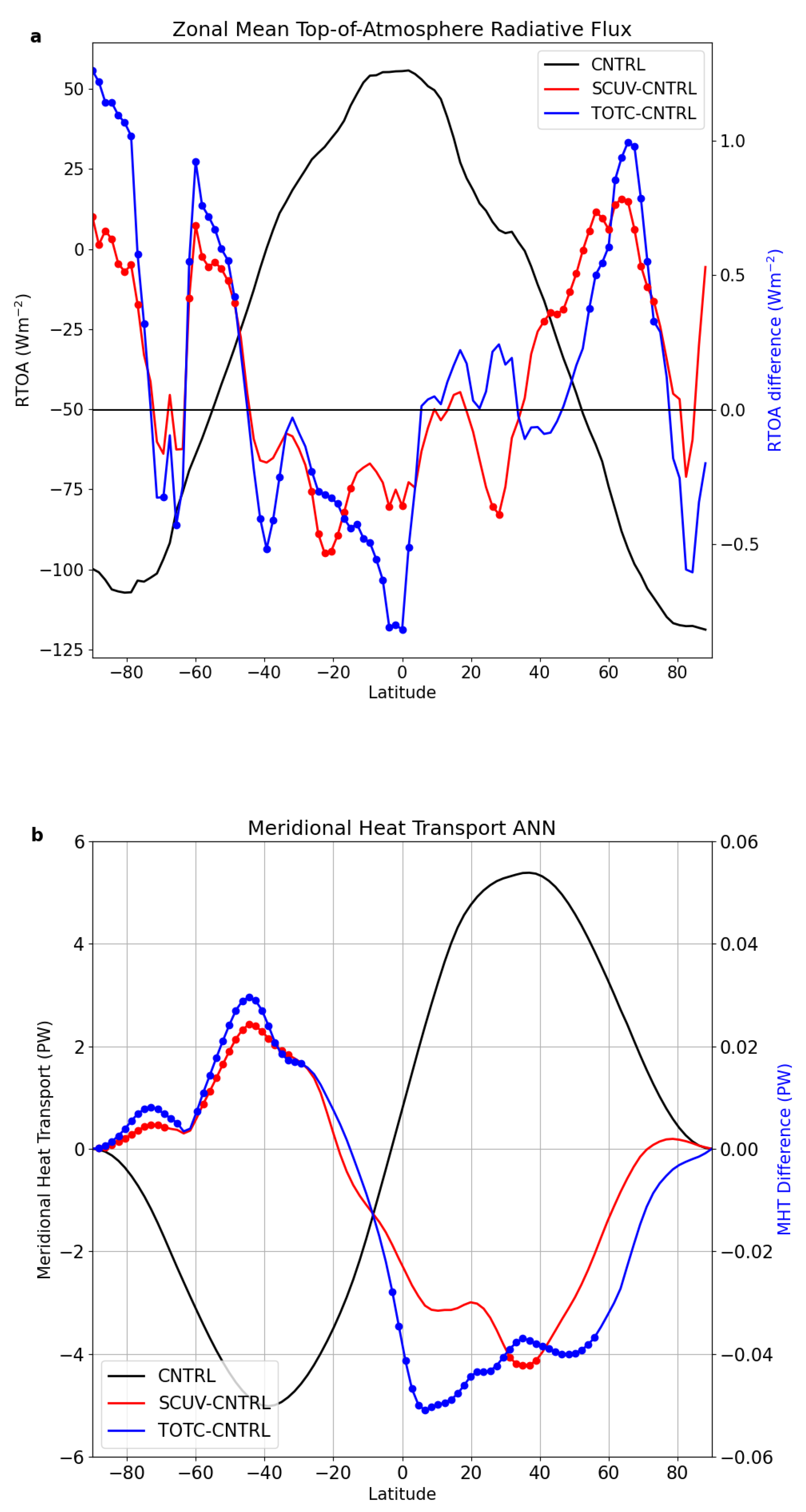
  • TOTC receives lower values of incoming radiation at the surface than SCUV. In TOTC, there is an absolute minimum MHT difference in the NH tropical region, suggesting that tropical regions not only receive less heat but are also unable to transport it poleward, even though, in this experiment, there is a higher thermal gradient caused by strong polar cooling. MHT differences are small but significant. The low values of MHT differences between SCUV, TOTC and CNTRL do not come as a surprise. Ref. [65] showed that MHT is nearly invariant in an ensemble of experiments spanning from the last glaciation to a world with CO2 quadrupled above the pre-industrial situation.
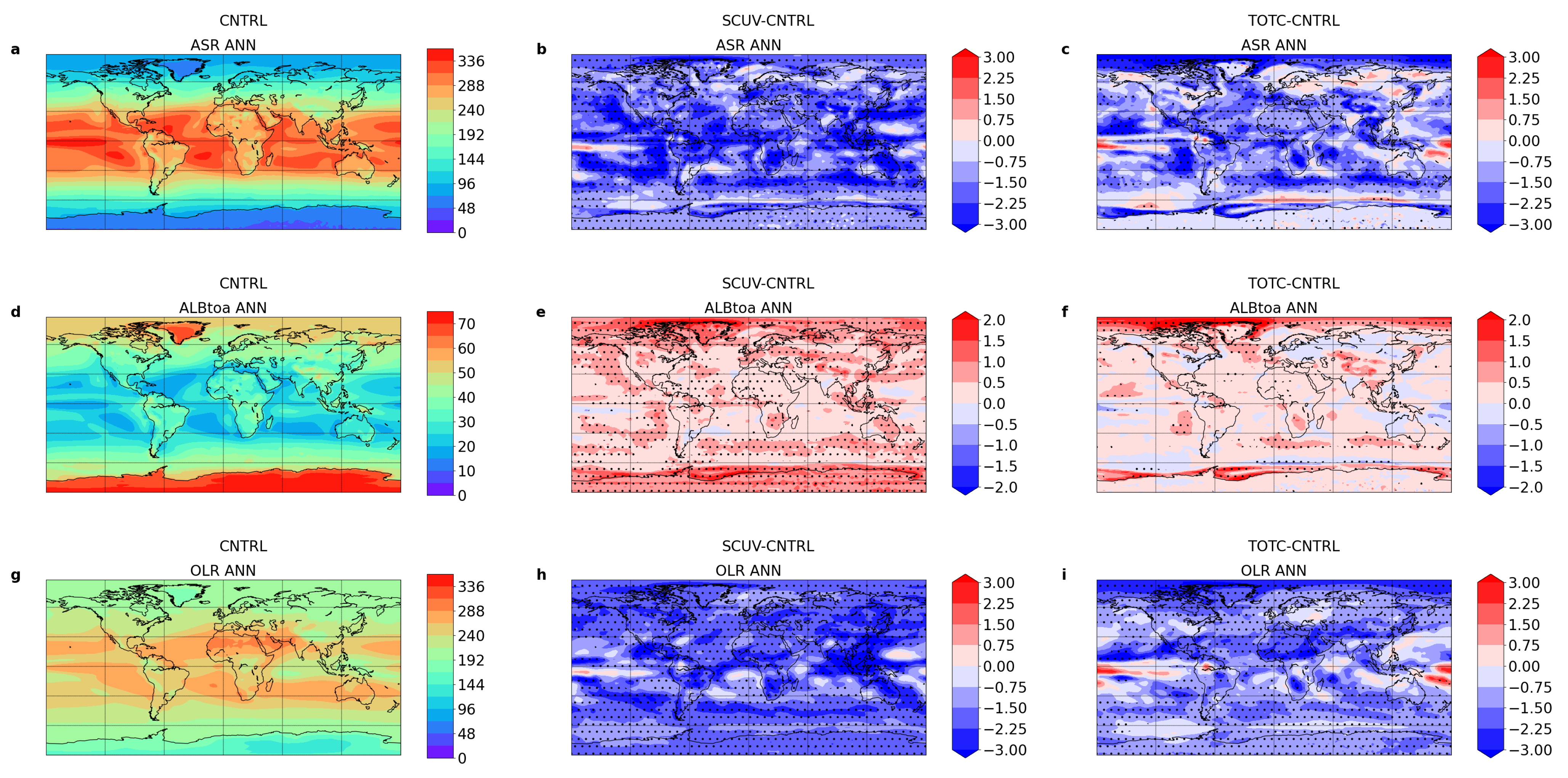
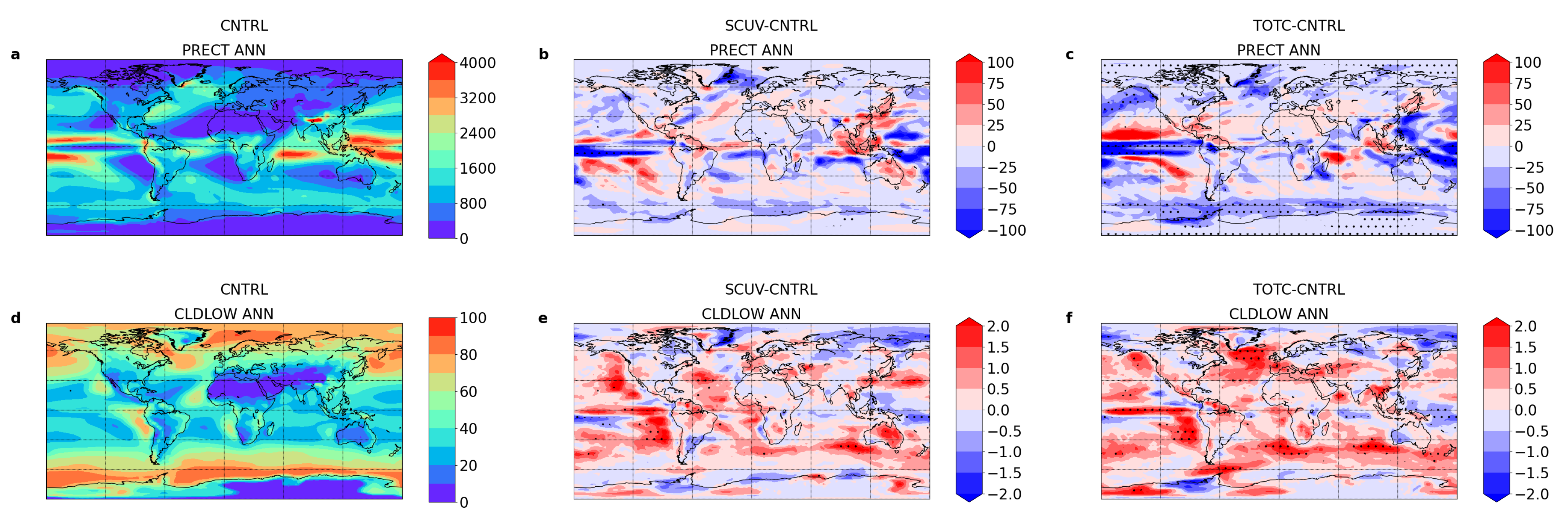
  • The difference in cloudiness among the experiments shows that the presence of feedback may also change the differential response. SCUV shows many more high clouds that reduce absorbed shortwave radiation by increasing the planetary albedo, as also shown by [71]. At the same time, they may contribute to warming the planet, whereas TOTC has more low clouds, which have a cooling effect on the climate as they increase outgoing longwave radiation. Low clouds over SH oceans would also play a role in the teleconnection between mid-latitudes and the tropical region [70];
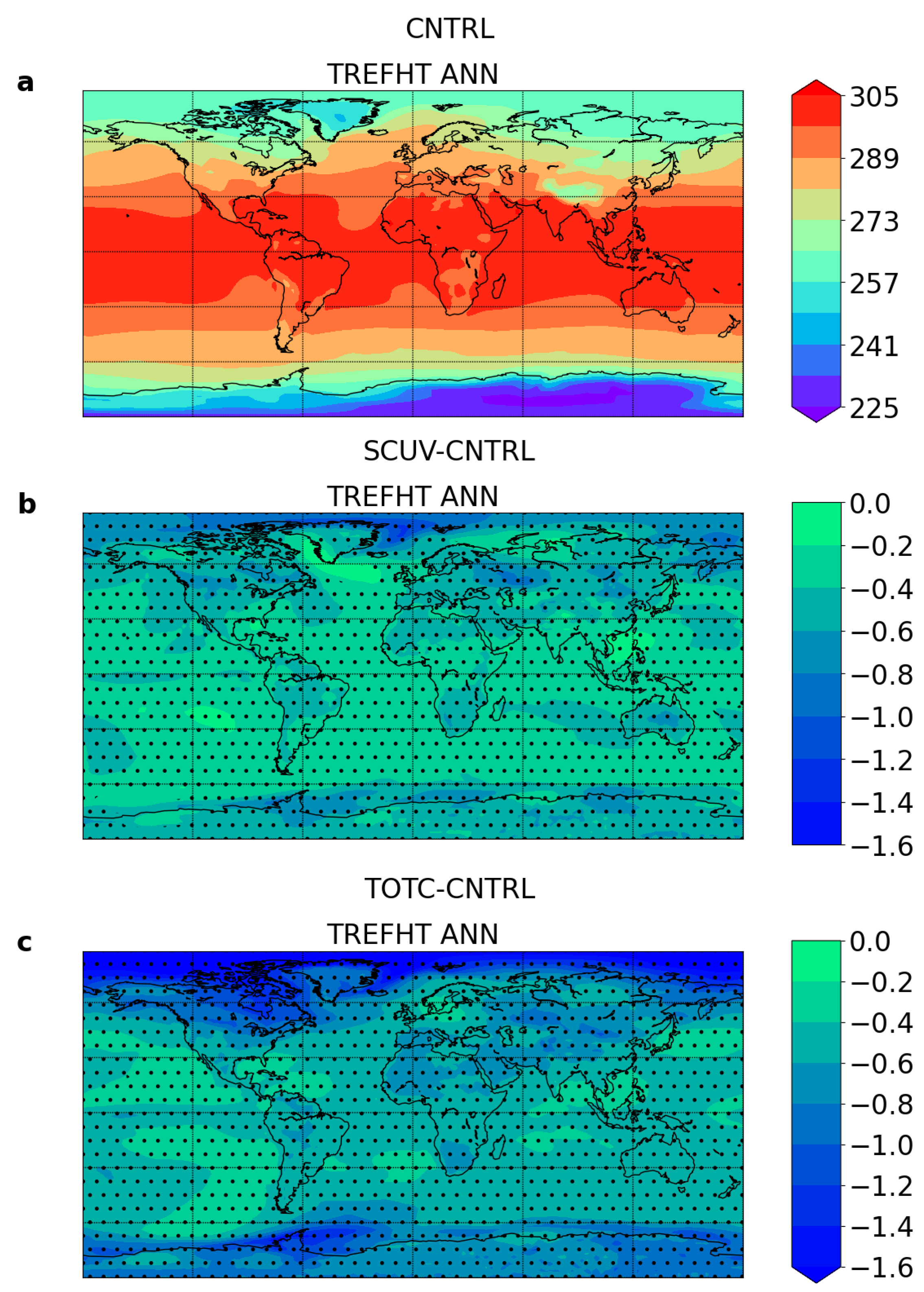
  • TOTC exhibits polar amplification in the Arctic region that cools the planet because of more ice fraction compared to CNTRL and SCUV. This larger cooling of the NH has consequences for the tropics as the HC and ITCZ are, in some way, correlated with cross-equatorial energy transport.
One of the points of debate on the influence of solar activity on climate has been over the so-called “bottom-up” and “top-down” mechanisms. Our results suggest that the “bottom-up” mechanism is prevalent not only under TOTC condition but even under SCUV conditions, confirming the results by [72], which used a more complex suite of experiments with different models. Moreover, SCUV shows that the UV reduction would make Earth’s climate warmer than TOTC, not only because of more shortwave arriving at the surface, but also because of high cloud feedback.
A few limitations of the present study need to be discussed briefly. The use of long periods with low TSI is a hypothesis needed to study the model response under those conditions. We also used Kp = 3 and Kp = 7 as extreme values associated with our minimum and maximum TSI. Both TSI and Kp in reality change continuously. In particular, TSI normally follows a 11-year cycle, and it is supposed to have a small impact, compared with the relatively long periods of a quiet Sun. The model uses the present atmospheric composition and does not aim to replicate past climate. As mentioned earlier, other studies have investigated the role of future climate with an increase in C O 2 , so the amount of C O 2 may be crucial in determining the impact on the temperature due to TSI reduction. The reconstruction of TSI and SSI is limited to that of Lean [1]. As shown in [73] there are twenty TSI reconstructions, and they may give conflicting results.
In this study, we have attempted to raise the awareness of the importance of UV solar irradiance as a climate forcing mechanism. There are still large uncertainties associated with the temporal evolution of UV irradiance over the last millennium, but new novel proxies for surface UV-B irradiance, based on the chemistry of pollen grains, are currently being developed [74]. Future research should, therefore, aim to combine such novel proxies, with coupled high-top climate models, incorporating fully interactive chemistry. Together, such measures will help further advance our understanding of how variations in solar UV irradiance may impact the climate system, both in past and possible future climates.

Supplementary Materials

The following supporting information can be downloaded at: https://www.mdpi.com/article/10.3390/cli12010001/s1.

Author Contributions

Conceptualization, N.T. and T.T.; methodology, N.T. and T.T.; software, N.T.; data curation, N.T.; writing—original draft preparation, N.T., T.T., Y.O. and O.H.O.; writing—review and editing, N.T., T.T., Y.O. and O.H.O.; supervision, T.T., O.H.O. and Y.O.; project administration, Y.O. and O.H.O.; funding acquisition, Y.O., O.H.O. and T.T. All authors have read and agreed to the published version of the manuscript.

Funding

This work was funded by the Norwegian Research Council through project 255276 (project SOLENA—Solar effects on natural climate variability in the North Atlantic and Arctic—The Research Council of Norway), Program for Space Research Project: 255276/E10, whose timeframe was 2017–2022. The simulations were performed on resources provided by UNINETT Sigma2—the National Infrastructure for High Performance Computing and Data Storage in Norway (NN9206K, NS9206K, NN9133K, NS9133K).

Data Availability Statement

The data were produced by the model WACCM v. 5.3, which was downloaded by https://www2.acom.ucar.edu/gcm/waccm, accessed on 28 September 2023. Software ConTrack v.0.3.0 used for Figure S2 is available at https://github.com/steidani/ConTrack, accessed on 31 January 2022. Some of the figures presented in this paper were created by modifying scripts present in Rose, Brian E. J. (9 November 2020). The Climate Laboratory https://brian-rose.github.io/ClimateLaboratoryBook/courseware/insolation.html, accessed on 31 January 2022. Because of amount of data, they are available from the authors under a reasonable request.

Acknowledgments

The authors acknowledge The Research Council of Norway for funding this work, Steinfield D. and Brian Rose to make their codes publicly accessible. The authors also thank two anonymous reviewers for their comments that improved the paper.

Conflicts of Interest

The authors declare no conflict of interest.

Abbreviations

The following abbreviations are used in this manuscript, and we kept the WACCM variable naming:
ASRAbsorbed Solar Radiation
ANNAnnual
CLDLOWLow Clouds
CNTRLControl Experiment
DJFDecember–January–February
DTCOREDynamical Heating Rate
EPEliassen Palm
FFlux
FDRFalse Discovery Rate
GSMGrand Solar Minim
ITCZInter-tropical Convergence Zone
JJAJune–July–August
HCHadley Cell
LHFLXLatent Heat Flux
LWLongwave
MAMMarch–April–May
MMMaunder Minimum
MSEMoist Static Energy
MHTMeridional Heat Transport
NHNorthern Hemisphere
OLROutgoing Longwave Radiation
PRECTTotal Precipitation
QRLHeating Rate of Longwave Radiation
QRSHeating Rate of Shortwave Radiation
RTOARadiation at the Top of the Atmosphere
SHSouthern Hemisphere
SWShortwave
LHFLXSensible Heat Flux
SCUVExperiment where the reduction is applied mainly to the ultraviolet spectrum
SOMSlab Ocean Model
SONSeptember–October–November
SSISolar Spectral Irradiance
SSTSea Surface Temperature
TTemperature
TOATop of the atmosphere
TOTCExperiment where the reduction is applied to all the radiation spectrum
TREFHT2 m Temperature
TSITotal Solar Irradiation
UZonal Component of wind
UVUltra-violet
VMeridional Component of Wind

References

  1. Lean, J. Evolution of the Sun’s Spectral Irradiance since the Maunder Minimum. Geophys. Res. Lett. 2000, 27, 2425. [Google Scholar] [CrossRef]
  2. Unruh, Y.C.; Solanki, S.K.; Fligge, M. Modelling solar irradiance variations: Comparison with observations, including line-ratio variations. In Workshop of the ISSI on Solar Variability and Climate; Springer: Berlin/Heidelberg, Germany, 2000; pp. 145–152. ISSN 0038-6308. [Google Scholar]
  3. Woods, T.N.; Rottman, G.J. Solar ultraviolet variability over time periods of aeronomic interest. In Comparative Aeronomy in the Solar System; Mendillo, M., Nagy, A., Waite, J., Eds.; American Geophysical Union: Washington, DC, USA, 2002; Volume 130, pp. 221–233. [Google Scholar]
  4. Lockwood, M. Was UV spectral solar irradiance lower during the recent low sunspot minimum? J. Geophys. Res. 2011, 116, D16103. [Google Scholar] [CrossRef]
  5. Woods, T.N.; Snow, M.; Harder, J.; Chapman, G.; Cookson, A. A different view of solar spectral irradiance variations: Modeling total energy of six-month intervals. Sol. Phys. 2015, 290, 2649. [Google Scholar] [CrossRef]
  6. Coddington, O.; Lean, J.; Pilewskie, P.; Snow, M.; Richard, E.; Kopp, G.; Lindholm, C.; DeLand, M.; Marchenko, S.; Haberreiter, M.; et al. Solar Irradiance variability: Comparisons of models and measurements. Earth Space Sci. 2019, 6, 2525–2555. [Google Scholar] [CrossRef]
  7. Krivova, N.A.; Solanki, S.K. Reconstruction of solar UV irradiance since 1974. Adv. Space Res. 2009, 114, D00I04. [Google Scholar] [CrossRef]
  8. Shapiro, A.I.; Schmutz, W.; Rozanov, E.; Schoell, M.; Haberreiter, M.; Shapiro, A.V.; Nyeki, S. A new approach to the long-term reconstruction of the solar irradiance leads to large historical solar forcing. Astron. Astrophys. 2011, 539, A67. [Google Scholar] [CrossRef]
  9. Schmidt, G.A.; Jungclaus, J.H.; Ammann, C.M.; Bard, E.; Braconnot, P.; Crowley, T.J.; Delaygue, G.; Joos, F.; Krivova, N.A.; Muscheler, R.; et al. Climate forcing reconstructions for use in PMIP simulations of the Last Millennium (v1.1). Geosci. Model Dev. 2012, 5, 185–191. [Google Scholar] [CrossRef]
  10. Lubin, D.; Miles, C.; Tytler, D. Ultraviolet flux decrease under a Grand Minimum from IUE Short-wavelength observation of solar analogs. Astron. Astrophys. 2017, 852, L4. [Google Scholar] [CrossRef]
  11. Wu, C.J.; Krivova, N.A.; Solanki, S.A.; Usoskin, I.G. Solar total and spectral irradiance reconstruction over the last 9000 years. Astron. Astrophys. 2018, 620, A120. [Google Scholar] [CrossRef]
  12. Mörner, N. The Approaching New Grand Solar Minimum and Little Ice Age Climate Conditions. Nat. Sci. 2015, 7, 510–518. [Google Scholar] [CrossRef]
  13. Luterbacher, J.; Rickli, R.; Xoplaki, E.; Tinguely, C.; Beck, C.; Pfister, C.; Wanner, H. The Late Maunder Minimum (1675–1715)—A key period for studying decadal scale climatic change in Europe. Clim. Chang. 2001, 49, 441–462. [Google Scholar] [CrossRef]
  14. Vaquero, J.M.; Svalgaard, L.; Carrasco, V.M.S.; Clette, F.; Lefévre, L.; Gallego, M.C.; Arlt, R.; Aparicio, A.J.P.; Richard, J.G.; Howe, R. A revised collection of sunspot group numbers. Sol. Phys. 2016, 91, 3061–3074. [Google Scholar] [CrossRef]
  15. Lehner, F.; Joos, F.; Raible, C.C.; Mignot, J.; Born, A.; Keller, K.M.; Stocker, T.F. Climate and carbon cycle dynamics in a CESM simulation from 850 to 2100 CE. Earth Syst. Dyn. 2015, 6, 411–434. [Google Scholar] [CrossRef]
  16. Velasco Herrera, V.M.; Mendoza, B.; Velasco Herrera, G. Reconstruction and Prediction of the Total Solar Irradiance; from the Medieval Warm Period to the 21st Century. New Astron. 2015, 34, 221–233. [Google Scholar] [CrossRef]
  17. Xoplaki, E.; Luterbacher, J.; Paeth, H.; Dietrich, D.; Steiner, N.; Grosjean, M.; Wanner, H. European spring and autumn temperature variability and change of extremes over the last half millennium. Geophys. Res. Lett. 2005, 32, L15713. [Google Scholar] [CrossRef]
  18. Christiansen, B.; Ljungqvist, F.C. The extra-tropical Northern Hemisphere temperature in the last two millennia: Reconstructions of low-frequency variability. Clim. Past 2012, 8, 765–786. [Google Scholar] [CrossRef]
  19. Wanner, H.; Pfister, C.; Brázdil, R.; Frich, P.; Frydendahl, K.; Jónsson, T.; Kington, J.; Lamb, H.H.; Rosenørn, S.; Wishman, E. Wintertime European circulation patterns during the Late Maunder Minimum cooling period (1675–1704). Theor. Appl. Climatol. 1995, 51, 167–175. [Google Scholar] [CrossRef]
  20. Barriopedro, D.; García-Herrera, R.; Huth, R. Solar modulation of Northern Hemisphere winter blocking. J. Geophys. Res. Atmos. 2008, 113, D14118. [Google Scholar] [CrossRef]
  21. Mellado-Cano, J.; Barriopedro, D.; García-Herrera, R.; Trigo, R.M.; Alvarez-Castro, M.C. Euro–Atlantic atmospheric circulation during the Late Maunder Minimum. J. Clim. 2018, 31, 3849–3863. [Google Scholar] [CrossRef]
  22. Foukal, P.; Ortiz, A.; Schnerr, R. Dimming of the 17th century sun. Astrophys. J. Lett. 2011, 733, L38. [Google Scholar] [CrossRef]
  23. Judge, P.G.; Lockwood, G.W.; Radick, R.R.; Henry, G.W.; Shapiro, A.I.; Schmutz, W.K.; Lindsey, C. Confronting a solar irradiance reconstruction with solar and stellar data. Astron. Astrophys. 2012, 544, A88. [Google Scholar] [CrossRef]
  24. Feulner, G.; Rahmstorf, S. On the effect of a new grand minimum of solar activity on the future climate on Earth. Geophys. Res. Lett. 2010, 37, L05707. [Google Scholar] [CrossRef]
  25. Abreu, J.A.; Beer, J.; Steinhilber, F.; Tobias, S.M.; Weiss, N.O. For how long will the current grand maximum of solar activity persist? Geophys. Res. Lett. 2008, 37, L20109. [Google Scholar] [CrossRef]
  26. Lockwood, M. Solar change and climate: An update in the light of the current exceptional solar minimum. Proc. R. Soc. A Math. Phys. Eng. Sci. 2010, 466, 303–329. [Google Scholar] [CrossRef]
  27. Egorova, T.; Schmutz, W.; Rozanov, E.; Shapiro, A.I.; Usoskin, I.; Beer, J.; Tagirov, R.V.; Peter, T. Revised historical solar irradiance forcing. Astron. Astrophys. 2018, 615, A85. [Google Scholar] [CrossRef]
  28. Krivova, N.A.; Solanki, S.K. Modelling of irradiance variations through atmosphere models. Mem. Soc. Astron. Ital. 2005, 76, 834–841. [Google Scholar]
  29. Lorenz, E.N. Forced and free variations of weather and climate. J. Atmos. Sci. 1979, 36, 1367–1376. [Google Scholar] [CrossRef]
  30. Haigh, J.D. A GCM study of climate change in response to the 11-year solar cycle. Q. J. R. Meteorol. Soc. 1999, 125, 871–892. [Google Scholar] [CrossRef]
  31. Meehl, G.A.; Arblaster, J.M.; Matthes, K.; Sassi, F.; van Loon, H. Amplifying the pacific climate system response to a small 11 year solar cycle forcing. Science 2009, 325, 1114–1118. [Google Scholar] [CrossRef]
  32. Gray, L.J.; Beer, J.; Geller, M.; Haigh, J.D.; Lockwood, M.; Matthes, K.; Cubasch, U.; Fleitmann, D.; Harrison, G.; Hood, L. Solar influences on climate. Rev. Geophys. 2010, 48, RG4001. [Google Scholar] [CrossRef]
  33. Kodera, K.; Kuroda, Y. Dynamical response to the solar cycle. J. Geophys. Res. Atmos. 2002, 107, ACL 5-1–ACL 5-12. [Google Scholar] [CrossRef]
  34. Haigh, J.D. The role of stratospheric ozone in modulating the solar radiative forcing of climate. Nature 1994, 370, 544–546. [Google Scholar] [CrossRef]
  35. Misios, S.; Mitchell, D.M.; Gray, L.J.; Tourpali, K.; Matthes, K.; Hood, L.; Schmidt, H.; Chiodo, G.; Thiéblemont, R.; Rozanov, E.; et al. Solar signals in CMIP-5 simulations: Effects of atmosphere-ocean coupling. Q. J. R. Meteorol. Soc. 2015, 142, 928–941. [Google Scholar] [CrossRef]
  36. Shindell, D.T.; Schmidt, G.A.; Mann, M.E.; Rind, D.; Waple, A. Solar forcing of regional climate change during the Maunder minimum. Science 2001, 294, 2149. [Google Scholar] [CrossRef] [PubMed]
  37. Scaife, A.A.; Ineson, S.; Knight, J.R.; Gray, L.J.; Kodera, K.; Smith, D.M. A mechanism for lagged North Atlantic climate response to solar variability. Geophys. Res. Lett. 2013, 40, 434–439. [Google Scholar] [CrossRef]
  38. Andrews, M.B.; Knight, J.R.; Gray, L.J. A simulated lagged response of the North Atlantic Oscillation to the solar cycle over the period 1960–2009. Environ. Res. Lett. 2015, 10, 054022. [Google Scholar] [CrossRef]
  39. Guttu, S.; Orsolini, Y.; Stordal, F.; Otterå, O.H.; Omrani, N.-E.; Tartaglione, N.; Verronen, P.T.; Rodger, C.J.; Clilverd, M.A. Impacts of UV Irradiance and Medium-Energy Electron Precipitation on the North Atlantic Oscillation during the 11-Year Solar Cycle. Atmosphere 2021, 21, 1029. [Google Scholar] [CrossRef]
  40. Anet, J.G.; Rozanov, E.V.; Muthers, S.; Peter, T.; Brönnimann, S.; Arfeuille, F.; Beer, J.; Shapiro, A.I.; Raible, C.C.; Steinhilber, F.; et al. Impact of a potential 21st century “grand solar minimum” on surface temperatures and stratospheric ozone. Geophys. Res. Lett. 2013, 40, 4420–4425. [Google Scholar] [CrossRef]
  41. Chiodo, G.; Garcia-Herrera, R.; Calvo, N.; Vaquero, J.M.; Anel, J.A.; Barriopedro, D.; Matthes, K. The impact of a future solar minimum on climate change projections in the Northern Hemisphere. Environ. Res. Lett. 2016, 11, 034015. [Google Scholar] [CrossRef]
  42. Jones, G.S.; Lockwood, M.; Stott, P.A. What influence will future solar activity changes over the 21st century have on projected global near-surface temperature changes? J. Geophys. Res. Atmos. 2012, 117, D05103. [Google Scholar] [CrossRef]
  43. Maycock, A.C.; Ineson, S.; Gray, L.J.; Scaife, A.A.; Anstey, J.A.; Lockwood, M.; Butchart, N.; Hardiman, S.C.; Mitchell, D.M.; Osprey, S.M. Possible impacts of a future grand solar minimum on climate: Stratospheric and global circulation changes. J. Geophys. Res. Atmos. 2015, 120, 9043–9058. [Google Scholar] [CrossRef] [PubMed]
  44. Meehl, G.A.; Arblaster, J.M.; Marsh, D.R. Could a future grand solar minimum like the maunder minimum stop global warming? Geophys. Res. Lett. 2013, 40, 1789–1793. [Google Scholar] [CrossRef]
  45. Ineson, S.; Maycock, A.C.; Gray, L.J.; Scaife, A.A.; Dunstone, N.J.; Harder, J.W.; Knight, J.R.; Lockwood, M.; Manners, J.C.; Wood, R.A. Regional climate impacts of a possible future grand solar minimum. Nat. Commun. 2015, 6, 7535. [Google Scholar] [CrossRef] [PubMed]
  46. Anet, J.G.; Muthers, S.; Rozanov, E.V.; Raible, C.C.; Stenke, A.; Shapiro, A.I.; Brönnimann, S.; Arfeuille, F.; Brugnara, Y.; Beer, J.; et al. Impact of solar versus volcanic activity variations on tropospheric temperatures and precipitation during the Dalton Minimum. Clim. Past 2014, 10, 921–938. [Google Scholar] [CrossRef]
  47. Arsenovic, P.; Rozanov, E.; Anet, J.; Stenke, A.; Schmutz, W.; Peter, T. Implications of potential future grand solar minimum for ozone layer and climate. Atmos. Chem. Phys. 2013, 18, 3469–3483. [Google Scholar] [CrossRef]
  48. Anet, J.G.; Muthers, S.; Rozanov, E.; Raible, C.C.; Peter, T.; Stenke, A.; Shapiro, A.I.; Beer, J.; Steinhilber, F.; Brönnimann, S.; et al. Forcing of stratospheric chemistry and dynamics during the Dalton Minimum. Atmos. Chem. Phys. 2013, 13, 10951–10967. [Google Scholar] [CrossRef]
  49. Rind, D.; Shindell, D.; Perlwitz, J.; Lerner, J.; Lonergan, P.; Lean, J.; McLinden, C. The relative importance of solar and anthropogenic forcing of climate change between the Maunder Minimum and the present. J. Clim. 2004, 17, 906–929. [Google Scholar] [CrossRef]
  50. Neale, R.B.; Chen, C.C.; Gettelman, A.; Lauritzen, P.H.; Park, S.; Williamson, D.L.; Conley, A.J.; Garcia, R.; Kinnison, D.; Lamarque, J.F.; et al. Description of the NCAR Community Atmosphere Model (CAM5); NCAR Tech. Note NCAR/TN-486+ STR; National Center for Atmospheric Research: Boulder, CO, USA, 2012. [Google Scholar]
  51. Marsh, D.R.; Mills, M.; Kinnison, D.; Lamarque, J.-F.; Calvo, N.; Polvani, L. Climate change from 1850 to 2005 simulated in CESM1(WACCM). J. Clim. 2013, 26, 7372–7391. [Google Scholar] [CrossRef]
  52. Marsh, D.R.; Garcia, R.R.; Kinnison, D.E.; Boville, B.A.; Sassi, F.; Solomon, S.C.; Matthes, K. Modeling the whole atmosphere response to solar cycle changes in radiative and geomagnetic forcing. J. Geophys. Res. Atmos. 2013, 112, 1–20. [Google Scholar] [CrossRef]
  53. Thiéblemont, R.; Matthes, K.; Omrani, N.-E.; Kodera, K.; Hansen, F. Solar forcing synchronizes decadal North Atlantic climate variability. Nat. Commun. 2015, 6, 8268. [Google Scholar] [CrossRef]
  54. Tartaglione, N.; Toniazzo, T.; Orsolini, Y.; Otterå, O.H. Impact of solar irradiance and geomagnetic activity on polar NOx ozone and temperature in WACCM simulations. J. Atmos. Sol. Terr. Phys. 2020, 209, 105398. [Google Scholar] [CrossRef]
  55. Schrijver, C.J.; Livingston, W.C.; Woods, T.N.; Mewaldt, R.A. The minimal solar activity in 2008–2009 and its implications for long-term climate modeling. Geophys. Res. Lett. 2011, 38, L06701. [Google Scholar] [CrossRef]
  56. Roth, R.; Joos, F. A reconstruction of radiocarbon production and total solar irradiance from the Holocene 14C and CO2 records: Implications of data and model uncertainties. Clim. Past 2013, 9, 1879–1909. [Google Scholar] [CrossRef]
  57. Lean, J.; Beer, J.; Bradley, R. Reconstruction of solar irradiance since 1610: Implications for climate change. Geophys. Res. Lett. 1995, 22, 3195–3198. [Google Scholar] [CrossRef]
  58. Lean, J.L. Estimating solar irradiance since 850 CE. Earth Space Sci. 2018, 5, 133–149. [Google Scholar] [CrossRef]
  59. Feulner, G. Are the most recent estimates for Maunder Minimum solar irradiance in agreement with temperature reconstructions? Geophys. Res. Lett. 2011, 38, L16706. [Google Scholar] [CrossRef]
  60. Peck, E.D.; Randall, C.E.; Harvey, V.L.; Marsh, D.R. Simulated solar cycle effects on the middle atmosphere: WACCM3 versus WACCM4. J. Adv. Model. Earth Syst. 2015, 7, 806–822. [Google Scholar] [CrossRef]
  61. Wilks, D.S. The stippling shows statistically significant grid-points. How research results are routinely overstated and overinterpreted, and what to do about it. Bull. Am. Meteorol. Soc. 2016, 97, 2263–2273. [Google Scholar] [CrossRef]
  62. Tartaglione, N.; Toniazzo, T.; Orsolini, Y.; Otterå, O.H. A note on the statistical evidence for an influence of geomagnetic activity on Northern Hemisphere seasonal-mean stratospheric temperatures using the Japanese 55-year Reanalysis. Ann. Geophys. 2020, 38, 545–555. [Google Scholar] [CrossRef]
  63. Kodera, K.; Thiéblemont, R.; Yukimoto, S.; Matthes, K. How can we understand the global distribution of the solar cycle signal on the Earth’s surface? Atmos. Chem. Phys. 2016, 16, 12925–12944. [Google Scholar] [CrossRef]
  64. Rao, J.; Yu, Y.Y.; Guo, D.; Shi, C.H.; Chen, D.; Hu, D.Z. Evaluating the Brewer–Dobson circulation and its responses to ENSO, QBO, and the solar cycle in different reanalyses. Earth Planet. Sci. 2019, 3, 166–181. [Google Scholar] [CrossRef]
  65. Donohoe, A.; Armour, K.C.; Roe, G.H.; Battisti, D.S.; Hahn, L. The Partitioning of Meridional Heat Transport from the Last Glacial Maximum to CO2 Quadrupling in Coupled Climate Models. J. Clim. 2020, 33, 4141–4165. [Google Scholar] [CrossRef]
  66. Kang, S.M.; Hawcroft, M.; Xiang, B.; Hwang, Y.-T.; Cazes, G.; Codron, F.; Crueger, T.; Deser, C.; Hodnebrog, Ø.; Kim, H.; et al. Extratropical–Tropical Interaction Model Intercomparison Project (Etin-Mip): Protocol and Initial Results. Bull. Am. Meteorol. Soc. 2019, 100, 2589–2606. [Google Scholar] [CrossRef]
  67. Hwang, Y.; Tseng, H.; Li, K.; Kang, S.M.; Chen, Y.; Chiang, J.C.H. Relative roles of energy and momentum fluxes in the tropical response to extratropical thermal forcing. J. Clim. 2021, 34, 3771–3786. [Google Scholar] [CrossRef]
  68. Feldl, N.; Bordoni, S. Characterizing the Hadley circulation response through regional climate feedbacks. J. Clim. 2016, 29, 613–622. [Google Scholar] [CrossRef]
  69. Kang, S.M.; Xie, S.-P.; Shin, Y.; Kim, H.; Hwang, Y.-T.; Stuecker, M.F.; Xiang, B.; Hawcroft, A.M. Walker circulation response to extratropical radiative forcing. Sci. Adv. 2020, 6, eabd3021. [Google Scholar] [CrossRef]
  70. Dong, Y.; Armour, K.C.; Battisti, D.S.; Blanchard-Wrigglesworth, E. Two-Way Teleconnections between the Southern Ocean and the Tropical Pacific via a Dynamic Feedback. J. Clim. 2022, 35, 6267–6282. [Google Scholar] [CrossRef]
  71. Donohoe, A.; Battisti, D.S. Atmospheric and Surface Contributions to Planetary Albedo. J. Clim. 2011, 24, 4402–4418. [Google Scholar] [CrossRef]
  72. Shindell, D.T.; Faluvegi, G.; Schmidt, G.A. Influences of solar forcing at ultraviolet and longer wavelengths on climate. J. Geophys. Res. Atmos. 2020, 124, e2019JD031640. [Google Scholar] [CrossRef]
  73. Connolly, R.; Soon, W.; Connolly, M.; Baliunas, S.; Berglund, J.; Butler, C.J.; Cionco, R.G.; Elias, A.G.; Fedorov, V.M.; Harde, H.; et al. How much has the Sun influenced Northern Hemisphere temperature trends? An ongoing debate. Res. Astron. Astrophys. 2021, 21, 131. [Google Scholar] [CrossRef]
  74. Jardine, P.E.; Fraser, W.T.; Gosling, W.D.; Roberts, C.N.; Eastwood, W.J.; Lomax, B.H. Proxy reconstruction of ultraviolet-B irradiance at the Earth’s surface, and its relationship with solar activity and ozone thickness. Holocene 2010, 30, 155–161. [Google Scholar] [CrossRef]
Figure 1. (a) SSI used for the CNTRL experiment (a) and SSI difference between the SSI forcing used in the experiments with reduced TSI (SCUV and TOTC experiments) in absolute [W·m 2 · nm 1 ] values (panel (b)) and relative [in percentage] values (panel (c)). The TSI value is 1357.8 W·m 2 for both sensitivity experiments. The gray, green and pink rectangles spanning horizontally from 120 to 200, 200 to 242, and 242 to 380 nm represent, respectively, three UV bands; the yellow rectangle represents the visible band 380–750 nm.
Climate 12 00001 g001
Figure 2. Seasonal climatology of the zonal-mean differences between SCUV and CNTRL of the following fields: temperature (K; (a,d,g,j)), zonal wind (m·s 1 ; (b,e,h,k)) and ozone (normalized on the seasonal mean, in percent; (c,f,i,l)). Stippling indicates a significant difference at a 5% level using Student’s t-test and the control of FDR. DJF, MAM, JJA and SON stand for (December–January–February, March–April–May, June–July–August, September–October–November).
Climate 12 00001 g002
Figure 3. Seasonal climatology of the zonal-mean of differences between SCUV and CNTRL of EP-flux horizontal and vertical components (arrows) and of EP-flux divergence (filled contour; m·s 1 · day 1 ; (a,d,g,j)), meridional (m·s 1 ; (b,e,h,k)) and vertical components (cm·s 1 ; (c,f,i,l)) of the residual circulation for DJF, MAM, JJA and SON. Positive values of the vertical component are upward. The vertical component of the EP-flux was scaled by the inverse of the pressure. Stippling indicates a significant difference at a 5% level using Student’s t-test and the control of FDR.
Climate 12 00001 g003
Figure 4. Seasonal climatology of the zonal-mean differences between TOTC and CNTRL of the following fields: temperature (K; (a,d,g,j)), zonal wind (m·s 1 ; (b,e,h,k)) and ozone (normalized on the seasonal mean, in percent; (c,f,i,l)). Stippling indicates a significant difference at a 5% level using Student’s t-test and the control of FDR. DJF, MAM, JJA and SON stand for (December–January–February, March–April–May, June–July–August, September–October–November).
Climate 12 00001 g004
Figure 5. Maps of the annual average 2 m temperature (TREFHT) for the control (a) and the differences between SCUV and CNTRL (b), and between TOTC and CNTRL (c). Units are in K. Stippling indicates a significant difference at a 5% level using Student’s t-test with control of FDR.
Climate 12 00001 g005
Figure 6. Climatological annual mean radiative heating rates for the control experiment of both shortwave (QRS; (a)) and longwave (QRL; (b)) components, overlaying the dynamical heating rate (DTCORE; contours). SCUV–CNTRL differences in QRS (c) and QRL (d) and DTCORE anomalies (contours). TOTC-CNTRL differences in QRS (e) and QRL (f) with DTCORE anomalies (contours). Units are in K day 1 . Stippling (hatching) indicates statistically significant differences in QRL and QRS (DTCORE) at a 5% level using Student’s t-test with the control of FDR.
Climate 12 00001 g006
Figure 7. Maps of the annual mean absorbed solar radiation (ASR; W·m 2 ; (a)) and the differences between SCUV and CNTRL (W·m 2 ; (b)), and between TOTC and CNTRL (W·m 2 ; (c)), planetary albedo (ALBtoa; %; (d)) and the differences between SCUV and CNTRL (%; (e)), and between TOTC and CNTRL (%; (f)) and Outgoing Longwave Radiation (OLR, W·m 2 ; (g)) and the differences between SCUV and CNTRL (W·m 2 ; (h)), and between TOTC and CNTRL (W·m 2 ; (i)). Stippling indicates a significant difference at the 5% level using Student’s t-test with control of FDR.
Climate 12 00001 g007
Figure 8. Annual mean radiative flux at the top of the atmosphere (RTOA in W·m 2 ; (a)) and meridional heat transport (in P W ; (b)) for CNTRL (black solid line) and the differences between SCUV and CNTRL (blue solid line) and between TOTC and CNTRL (red line). The dots indicate statistically significant differences at the 5% level with the control of FDR.
Climate 12 00001 g008
Figure 9. Annual mean changes in SCUV-CNTRL (a), TOTC-CNTRL (b) of zonal mean temperature (K, shaded) and zonal average of zonal wind (m·s 1 , contours).The dots indicate statistically significant differences at the 5% level with the control of FDR.
Climate 12 00001 g009
Figure 10. Maps of the annual mean precipitation (PRECT; mm; (a)) and the differences between SCUV and CNTRL (mm; (b)), and between TOTC and CNTRL (mm; (c)), and of the total low cloud l (CLDLOW; %; (d)) and the differences between SCUV and CNTRL (%; (e)), and between TOTC and CNTRL (%; (f)). Stippling indicates a significant difference at the 5% level using Student’s t-test with control of FDR.
Climate 12 00001 g010
Figure 11. Heat surface flux in W·m 2 for CNTRL (a), and differences between SCUV and CNTRL (b) and between TOTC and CNTRL (c). Flux terms: SWsfc (shortwave at surface), LWsfc (longwave at surface), NetRad (net upward radiation from surface), LHFLX (latent heat flux), SHFLX (sensible heat flux), Net (net upward surface heat flux). Positive values denote outgoing heat flux, negative values incoming net flux.
Climate 12 00001 g011
Figure 12. Monthly averaged ice fraction (%) (a) and 2 m temperature (K) (b) differences between sensitivity (SCUV and TOTC) and CNTRL experiments for September (blue), October (green) and November (brown). Dots indicate statistically significant differences at the 5% level with the control of FDR.
Climate 12 00001 g012
Disclaimer/Publisher’s Note: The statements, opinions and data contained in all publications are solely those of the individual author(s) and contributor(s) and not of MDPI and/or the editor(s). MDPI and/or the editor(s) disclaim responsibility for any injury to people or property resulting from any ideas, methods, instructions or products referred to in the content.

