The Solar Radiation Climate of Saudi Arabia

Abstract

In the present work, we investigate the solar radiation climate of Saudi Arabia, using solar radiation data from 43 sites in the country covering the period 2013–2021. These data include hourly values of global, G, and diffuse, G_d, horizontal irradiances from which the direct, G_b, horizontal irradiance is estimated. The diffuse fraction, k_d; the direct-beam fraction, k_b; and the ratio k_e = G_d/G_b, are used in the analysis. Solar maps of the annual mean G, G_d, k_d, k_b, and k_e are prepared for Saudi Arabia under all- and clear-sky conditions, which show interesting but explainable patterns. Additionally, the intra-annual and seasonal variabilities of these parameters are presented, and regression equations are provided. We find that G_b has a negative linear relationship with k_d; the same applies to G with respect to k_d or the latitude, φ, of the site. It is shown that k_d and k_b can reflect the scattering and absorption effects of the atmosphere on solar radiation, respectively; therefore, they can be used as atmospheric scattering and absorption indices. Part of the analysis considers the defined solar energy zones in Saudi Arabia.

1. Introduction

Solar radiation is the primary source for life on Earth as it controls atmospheric environment [1], terrestrial ecosystems [2], and terrestrial climate [3]. Solar radiation is the most abundant renewable energy source (RES) on Earth; other RES types are wind, tides, and geothermy. Exploitation of the solar RES type intensively started in the 1980s for converting solar radiation into water heating (solar thermosyphons). Nevertheless, the main application of solar energy is nowadays for photovoltaic (PV) installations [4,5], which started almost 20 years ago.

The fluctuations in the solar radiation amount at any location on Earth depend upon changes in the atmospheric constituents [6], variations in the amount and texture of clouds [7], as well as the Sun–Earth geometrical variability (the well-known Milankovitch theory [8]). Therefore, clouds and atmospheric aerosols are two factors that play significant roles in determining the solar radiation climate at a site on the scale of decades. These two factors vary in space and time, causing subsequent variability in solar radiation [9].

The solar radiation climate at a location provides information about the levels and trends of the three solar radiation components (global, diffuse, and direct) over a relatively long period of time (usually about 10 years or longer). The international literature contains works about the solar radiation climate at various locations on Earth; indicative studies exist for Barcelona, Spain [10]; Alaska, USA [11]; central Europe [12]; California, USA [13]; Malawi [9]; Sweden [14]; Thailand [15]; Africa [16]; and Greece [5,17,18,19,20].

In particular, some places around the world have a climate similar to that of Saudi Arabia (semi-arid desert [21]), and some information about their solar radiation climate has been provided. The interest in such areas is high because of their high solar potential but their lack of solar radiation measuring stations. Therefore, modeling of solar radiation has been used as substitute for solar measurements in order to provide crucial information for solar applications, mostly photovoltaic (PV). One such a place is the Atacama Desert, extending across Chile, Peru, Bolivia, and northern Argentina. Marzo et al. [22] developed an artificial neural network (ANN) model to estimate daily solar radiation values suitable for the operation of PV systems; the inputs used for the implementation of the model were the daily minimum and maximum air temperatures and extraterrestrial solar radiation. The ANN model was validated against data from deserts in Chile, Israel, Saudi Arabia, South Africa, and Australia. The results showed that the average relative root mean square deviation was 13%, the average relative mean bias error was less than 4%, and the average correlation coefficient was about 0.8.

Behar et al. [23] investigated the performance of 38 clear-sky direct solar radiation models in the Chilean Atacama Desert and found that 6 of those produced the best results. Gairaa et al. [24] presented a solar radiation forecasting method for daily values using nonlinear autoregressive neural networks (NAR) for the site of Ghardaïa in a desert in south Algeria. The validated results showed an improvement in the NAR model over the autoregressive-moving average method of 23.89% in terms of the mean absolute error and a decrease in the root mean square error of about 15.50%. Diabate et al. [16] studied the solar climate of Africa; they divided the continent in 20 climatic zones, among which zones with numbers 4 (high Sahara plateaus), 12 (desert areas in Sahara, Libya, Egypt), 13 (western Sahara), 14 (northern Sahara), 16 (deserts of Kalahari and Namib), and 18 (southeastern Sahel) were included.

In Saudi Arabia, no specialized and detailed study has been made for the whole country, though several works have been conducted for the solar radiation levels at certain locations or regions in the country. The first work on the solar availability at certain sites in Saudi Arabia dates to the 1980s and 1990s [21,22,23,24,25,26]. More recent studies have tried to determine the solar potential over Saudi Arabia [25,26,27,28], but they either have failed in providing much detail about the solar availability or have given incomplete information about the solar radiation climate of the country.

The only projects that have provided maps of the solar radiation levels over Saudi Arabia in their reports are the following:

• The Saudi Arabian National Centre for Science and Technology initiated the Renewable Resource Atlas of the Kingdom of Saudi Arabia in the early 1980s. In 1999, a new Solar Radiation Atlas for Saudi Arabia was generated in cooperation with The Centre and the U.S. Department of Energy [29,30]. Later in 2013, a new Renewable Resource Atlas for Saudi Arabia was produced [30] without the inclusion of solar maps.
• The first Solar Radiation Atlas for the Arab World was derived in 2004 [31] and included Morocco, Algeria, Tunisia, Egypt, Saudi Arabia, the UAE, Kuwait, Syria, Jordan, and Bahrain; this Atlas depicts the distribution of the monthly and annual mean solar irradiation in the territory. Later, in 2019, the World Bank [32] presented a solar atlas for the world including Saudi Arabia, but not much detail was provided for the country.

From the above, it is seen that no study or project has investigated the solar radiation climate of Saudi Arabia. This gap is, therefore, filled by the present study for the first time. Apart from the three solar radiation components, the following parameters were included in the analysis: the diffuse fraction, k_d, i.e., the diffuse-to-global horizontal solar irradiance ratio, G_d/G; and the direct-beam fraction, k_b, i.e., the direct-to-global horizontal solar irradiance ratio, G_b/G, were used in the present study as in [20]. Additionally, the diffuse-to-direct-beam horizontal solar radiation ratio, k_e = G_d/G_b, was defined and used in the present work.

The diffuse fraction has been used by various researchers in an effort to develop solar radiation models with the purpose of calculating the diffuse solar radiation, e.g., [33,34,35], a solar radiation component that is difficult to estimate due to various reasons (clouds, atmospheric turbidity, etc.). Moreover, the k_d parameter is associated with the atmospheric scattering mechanism in the atmosphere [19,20]. In this context, k_b can be examined as an absorption index of solar radiation in the atmosphere [19]. Finally, k_e was used in the present work as it gives information about the percentage contribution of both the G_d and G_b solar radiation components to solar applications over an area and, more specifically, to PV installations [36].

2. Materials and Methods

The analysis in this study was based on data gathered in the frame of the Renewable Resource Atlas (RRA) for Saudi Arabia, which was launched in 2013 as part of the King Abdullah City for Atomic and Renewable Energy’s (K.A.CARE’s) Renewable Resource Monitoring and Mapping (RRMM) program [37,38]. The RRMM program funded the establishment of 47 solar radiation stations throughout Saudi Arabia. The collection of data started in August 2013 and continued to the end of August 2021; this duration is not the same at all of the stations of the program, which means that gaps exist. To overcome this problem, those stations with the fewest gaps in their databases or with a database completeness of over 95% were selected. This criterion resulted in adopting 43 out of the 47 data bases. The 43 sites are shown in

Table 1. The 43 sites involved in the study. The names of the locations are given in alphabetical order. The geographical longitude, λ; and the geographical latitude, φ, are in degrees (°); E = east of the Greenwich meridian; N = northern hemisphere; amsl = above mean sea level.

Site Number	Site Name/Site Altitude (m amsl)	λ (° E)	φ (° N)
1	Abha/2173	21.383	38.617
2	Afif/1060	25.933	40.850
3	Al Aflaaj/567	22.800	39.067
4	Al Ahsa/170	21.283	37.917
5	Al Bada/1680	21.417	38.133
6	Al Dawadmi/955	20.988	39.158
7	Al Dhahran/75	26.150	38.350
8	Al Farshah/1094	26.496	41.348
9	Al Hanakiyah/873	22.044	40.802
10	Al Jouf/680	23.750	37.900
11	Al Jubail/89	20.817	39.700
12	Al Khafji/13	25.183	35.333
13	Al Kharj/438	22.000	37.067
14	Al Qunfudhah/20	25.333	35.120
15	Al Wajh/21	29.576	36.142
16	Arar/583	21.283	40.450
17	Dammam/28	19.917	39.617
18	Duba/45	25.407	41.122
19	Farasan/16	21.783	40.283
20	Hada Al Sham/245	23.017	36.133
21	Hafar Al Batin/383	22.400	38.850
22	Hagl/36	22.450	39.650
23	Hail/928	26.600	39.067
24	Jeddah/65	25.233	39.917
25	Al Majma’ah/718	21.700	36.833
26	Mecca/295	22.967	40.517
27	Medina/643	24.475	36.697
28	Najran/1187	25.533	37.100
29	Osfan/119	26.531	41.501
30	Al Qassim/688	28.117	36.400
31	Rania/933	26.917	37.700
32	Riyadh1/688	23.567	41.083
33	Riyadh2/779	26.100	35.120
34	Riyadh3/895	24.550	38.900
35	Shaqra/804	21.117	35.550
36	Sharurah/760	23.917	37.967
37	Tabuk/781	23.550	38.317
38	Taif/1518	25.433	36.417
39	Thuwal/5	23.320	38.322
40	Timaa/844	21.768	39.556
41	Umluj/10	22.400	37.533
42	Wadi ad Dawasir/671	24.886	41.130
43	Yanbu/17	20.900	37.783

, and their location on the map of Saudi Arabia is shown in Figure 1.

The parameters measured at the RRMM stations were the global horizontal irradiance, G (Wm⁻²); the diffuse horizontal irradiance, G_d (Wm⁻²); the direct-normal irradiance, G_bn (Wm⁻²); and the air temperature, T (degrees Celcius). The parameters exploited in the present study were G and G_d: their symbols follow the ISO 9488:2022 Solar energy—Vocabulary. Both solar radiation components were measured at all stations with KIPP & ZONEN’s CMP21 pyranometers having an accuracy of ±2%. The diffuse radiation was recorded with the aid of a rotating shadow band over the pyranometer (for more information, see [28]). The data were sampled every minute, and hourly averages were later computed offline in the frame of the RRMM program. The equipment was maintained daily according to the Technical Reports for each station within the RRMM program. The pyranometers were new at the beginning of the measuring period; nevertheless, they were exchanged with spares, as needed, to maintain the validity of the manufacturer’s 2-year warranty. More about the solar radiation equipment in the RRMM program can be found in [28].

Hourly values of solar radiation were preferred in the present study instead of daily or even monthly ones, because we wanted to grasp any small temporal variation in their levels; daily and monthly averages smooth out any effect of weather on solar radiation.

The hourly solar radiation values were inspected for errors by applying the criteria: G or G_d > 0 Wm⁻², and G_d ≤ G. Values not satisfying the criteria were discarded from further analysis. Hourly values of direct horizontal irradiance, G_b (Wm⁻²), were computed by the difference G − G_d. Further calculations referred to the diffuse fraction, k_d = G_d/G; the direct-beam fraction, k_b = G_b/G; and the ratio G_d/G_b introduced in [36], denoted as k_e in the present paper. Any hourly gaps in any parameter, any month, or any site were filled in by the average of the parameter for the same hour from the other same months in the data base. In the analysis of the data, a distinction between situations under all- and clear-sky conditions was made; the criteria for this classification were adopted from [39]: 0 < k_d ≤ 0.26 for clear skies, and 0 < k_d ≤ 1 for all skies. In this way, error-free and 100% complete data bases were established for the 43 sites covering the period 2013–2021 (9 years). Finally, annual, seasonal, and monthly values were calculated for all parameters, all sites, and both sky conditions.

Figure 1. Distribution of the 43 sites across Saudi Arabia. The numbers refer to those in column 1, Table 1. The country was divided into 3 solar energy zones (SEZ): SEZ-A, SEZ-B, and SEZ-C, according to their solar potential estimated in a study by Farahat et al. [40].

Figure 1. Distribution of the 43 sites across Saudi Arabia. The numbers refer to those in column 1, Table 1. The country was divided into 3 solar energy zones (SEZ): SEZ-A, SEZ-B, and SEZ-C, according to their solar potential estimated in a study by Farahat et al. [40].

The features of the above 5 parameters (G, G_d, k_d, k_b, and k_e) in characterizing the solar radiation climate of Saudi Arabia are as follows:

• G expresses the overall solar intensity arriving at the surface of the Earth and corresponds to the total extinction (absorption and scattering) of the solar rays passing through the atmosphere.
• G_d refers to the scattering of the solar rays in the atmosphere.
• k_d indicates the participation of the scattering process to the total extinction of solar radiation during its passage through the atmosphere; therefore, it can be used here as an atmospheric scattering index [19,20].
• k_b mostly corresponds to the participation of the absorption process to the total extinction of solar light, and it can become synonymous with an atmospheric absorption index [19,20].
• k_e = G_d/G_b is the atmospheric extinction index, because it denotes the contribution of the scattering (by G_d) and absorption (by G_b) mechanisms in the atmosphere; dividing the ratio by G gives k_e = k_d/k_b. This index is also useful as it denotes the significant fractional amount of each solar component in solar harvesting [36].

In the analysis in this work, some statistical indicators were employed; they describe the performance of nonlinear regression fits to the seasonal or monthly mean values of the G, G_d, k_b, k_d, and k_e parameters. These indicators were the average, ave; the standard deviation, σ; the root mean square error, RMSE; the mean absolute error, MAE; the index of agreement or Willmott’s index [41], d; the correlation coefficient, r; and the coefficient of determination, R². Their definitions are, respectively, given by the following analytical expressions:

$$\mathrm{ave} =\frac{{{\displaystyle \sum }}_{\mathrm{i}=1}^{\mathrm{N}}{\mathrm{x}}_{\mathrm{i}}}{\mathrm{N}}$$

(1)

$$\mathsf{\sigma }=\frac{{{\displaystyle \sum }}_{\mathrm{i}=1}^{\mathrm{N}}{({\mathrm{x}}_{\mathrm{i}}-\stackrel{-}{\mathrm{x}})}^2}{\mathrm{N}}$$

(2)

$$\mathrm{RMSE}=\sqrt{{\displaystyle \sum }_{\mathrm{i}=1}^{\mathrm{N}}\frac{{({\mathrm{O}}_{\mathrm{i}}-{\mathrm{E}}_{\mathrm{i}})}^2}{\mathrm{N}}}$$

(3)

$$\mathrm{MAE}=\frac{{{\displaystyle \sum }}_{\mathrm{i}=1}^{\mathrm{N}}|{\mathrm{O}}_{\mathrm{i}}-{\mathrm{E}}_{\mathrm{i}}|}{\mathrm{N}}$$

(4)

$$\mathrm{d}=1-\frac{{{\displaystyle \sum }}_{\mathrm{i}=1}^{\mathrm{N}}{({\mathrm{O}}_{\mathrm{i}}-{\mathrm{E}}_{\mathrm{i}})}^2}{{{\displaystyle \sum }}_{\mathrm{i}=1}^{\mathrm{N}}{(|{\mathrm{E}}_{\mathrm{i}}-\stackrel{-}{\mathrm{O}}|+|{\mathrm{O}}_{\mathrm{i}}-\stackrel{-}{\mathrm{O}}|)}^2}$$

(5)

$$\mathrm{r}=\frac{{{\displaystyle \sum }}_{\mathrm{i}=1}^{\mathrm{N}}({\mathrm{O}}_{\mathrm{i}}-\stackrel{-}{\mathrm{O}})·({\mathrm{E}}_{\mathrm{i}}-\stackrel{-}{\mathrm{E}})}{\sqrt{{{\displaystyle \sum }}_{\mathrm{i}=1}^{\mathrm{N}}{({\mathrm{O}}_{\mathrm{i}}-\stackrel{-}{\mathrm{O}})}^2·{{\displaystyle \sum }}_{\mathrm{i}=1}^{\mathrm{N}}{({\mathrm{E}}_{\mathrm{i}}-\stackrel{-}{\mathrm{E}})}^2}}$$

(6)

$${\mathrm{R}}^2=1-\frac{{{\displaystyle \sum }}_{\mathrm{i}=1}^{\mathrm{N}}{({\mathrm{O}}_{\mathrm{i}}-{\mathrm{E}}_{\mathrm{i}})}^2}{{{\displaystyle \sum }}_{\mathrm{i}=1}^{\mathrm{N}}{({\mathrm{O}}_{\mathrm{i}}-\stackrel{-}{\mathrm{O}})}^2}$$

(7)

where E_i and O_i denote the estimated (modelled) and observed (measured) values, respectively; and x_i is the value of a variable in its data series (in this case, either O_i or E_i); the bar over x, O, or E implies the average of x, observed, or estimated time series; the subscript i refers to any season or month of the year (i = 1,…,4 or i = 1,…,12, respectively); N is the number of data points in the time series (N = 4 for seasons; N = 12 for months).

σ expresses the average amount of variability in the data set, i.e., it informs, on average, about how far each value lies from the mean. The RMSE is the standard deviation of the residuals (i.e., estimated–observed) values and is a measure of how far the estimated data points are from the model (regression line). The lower the RMSE, the closer the estimated values to the regression curve. The MAE is the average absolute error between the measured and estimated values; the closer the MAE to 0, the more accurate the model (regression line). d represents the ratio of the mean square error to the potential error and is a standardized measure of the degree of the model (regression line) prediction; it varies between 0 (no agreement at all) and 1 (perfect match). r is a measure of the strength of the relationship between the measured and estimated time series; it varies between −1 (complete anticorrelation) to 0 (no correlation at all) and +1 (complete correlation). R² provides information about the goodness-of-fit of a model; it varies between 0 (no match at all) and 1 (perfect match).

3. Results

3.1. Annual Variation

Figure 2 shows the variation in the annual mean values of G and G_d for all- and clear-sky conditions across all 43 sites in Saudi Arabia. The data points in the graphs are presented in different colors according to the SEZ to which they belong (SEZ-A, red; SEZ-B, orange; SEZ-C, green). The ±1σ bands (σ = standard deviation) around the average values in each SEZ are also shown and are indicated by vertical double-arrowed lines. From these graphs, interesting features appear, which we comment on in the following.

Under all skies (Figure 2a), only 3 G data points out of 23 (13%) lie outside the SEZ-A ±1σ band, 4 out of 18 (≈22%) outside the SEZ-B ± 1σ band, and none outside the SEZ-C ±1σ band. This finding verifies the decision of Farahat et al. [40] to define three solar energy zones for Saudi Arabia. Moreover, a higher average annual G value (≈463 Wm⁻²) occurred in SEZ-A, a lower one in SEZ-B (≈456 Wm⁻²), and an even lower one in SEZ-C (≈450 Wm⁻²), as expected, because of the increasing geographical latitude from SEZ-A to SEZ-C and, therefore, decreasing solar radiation. A third observation is that the width of the ±1σ band for SEZ-A is comparable to that for SEZ-B, but each of them is greater than the standard deviation band of SEZ-C. The larger SEZ-A and SEZ-B ±1σ bands mean that the variability in the annual G values is greater than that in SEZ-C. This observation comes from the finding that the sites in SEZ-A or SEZ-B are located in various environments (deserts, plains, and coasts) and at various altitudes (low and high) compared with those in SEZ-C; this environmental mosaic affects the solar radiation measured on the ground (i.e., the G). Another reason may be the very low number of sites within SEZ-C (two), resulting in a low standard deviation due to the comparable annual values of these two sites. Similar characteristics can be observed for the G_d solar component in Figure 2c: (i) 5 G_d data points outside the SEZ-A ±1σ band (35%), 3 outside the SEZ-B band (17%), and none outside the SEZ-C band; (ii) comparable ±1σ band widths for SEZ-A and SEZ-B, which are both larger than the SEZ-C one; (iii) decreasing average annual G_d values from SEZ-A (≈172 Wm⁻²) to SEZ-B (≈162 Wm⁻²) and SEZ-C (≈144 Wm⁻²); greater variability in the SEZ-A annual G_d values than in the other two SEZs.

Under clear skies (Figure 2b), 6 G data points are outside the SEZ-A ±1σ band (26%), 4 outside the SEZ-B ±1σ band (≈22%), and none outside the SEZ-C one. The other characteristics found in the all-sky case are found here, too. Furthermore, the average annual values are ≈779 Wm⁻² for SEZ-A, ≈749 Wm⁻² for SEZ-B, and ≈708 Wm⁻² for SEZ-C. In the case of the G_d component, its average annual values are as follows: ≈157 Wm⁻² for SEZ-A, ≈147 Wm⁻² for SEZ-B, and ≈127 Wm⁻² for SEZ-C. Six G_d values are outside the SEZ-A ±1σ band (≈26%), 4 outside the SEZ-B ±1σ band (≈22%), and none outside the SEZ-C band.

A general conclusion from the above results can be then drawn as follows: the difference in the annual mean G or G_d values across the three SEZs dictate the need to consider them separately in the rest of the study. In this context, Figure 3 shows the different methods of presenting the annual means and standard deviations. The vertical bars indicate the average values, and the error bars indicate the standard deviations. Here, a black bar was added, which corresponds to all sites irrespective of the SEZ. Comparable breadths of the ±1σ bands in the cases of SEZ-All, SEZ-A, and SEZ-B are found. The average value for SEZ-All is between those for SEZ-A and SEZ-B. This was expected, as the weights of the two SEZ-C sites in the averaging process are small compared with those of the sites in the other two solar energy zones.

3.2. Monthly Variation

Figure 4 shows the intra-annual variation in G under all- (left panels, i.e., Figure 4a,c,e,g) and clear- (right panels, i.e., Figure 4b,d,f,h) sky conditions. More specifically, the diagrams for SEZ-All (Figure 4a,b), SEZ-A (Figure 4c,d), SEZ-B (Figure 4e,f), and SEZ-C (Figure 4g,h) are presented. The black lines are the monthly mean G values, while the red and blue lines represent the upper and lower limits of the ±1σ band, respectively, as in the case of the annual values. The green dotted curves are sixth-order polynomial fits to the mean curves. In all cases, the polynomial curves have a very high R², implying an almost perfect fit to the mean values (see

Table 2. Estimation of the monthly mean values of G (Wm⁻²) and G_d (Wm⁻²), which are averages over the period 2013–2021, for all 43 sites in SEZ-All, or those sites that belong to the separate zones SEZ-A, SEZ-B, and SEZ-C. t is month (1 = January, 12 = December); statistical estimators for the model’s goodness-of-fit: RMSE (Wm⁻²), MAE (Wm⁻²), d, r, and R². All statistical results were computed with the MICROSOFT’s Excel 2021 functions.

Parameter	Regression Equation
Sky Type, SEZ	RMSE, MAE, d, r, R2
G	G = 0.0221t6 − 0.8464t5 + 12.5370t4 − 89.9070t3 + 309.3000t2 − 383.7500t + 758.2000
clear, All	2.9578, 1.7792, 0.9989, 0.9996, 0.9992
Gd	Gd = 0.0075t6 − 0.2889t5 + 4.3297t4 − 31.6383t3 + 113.5537t2 − 162.7976t + 186.5065
clear, All	2.2509, 1.5970, 0.9914, 0.9966, 0.9931
G	G = 0.0084t6 − 0.3101t5 + 4.3832t4 − 29.8840t3 + 96.3720t2 − 93.9490t + 402.6700
all, All	5.2575, 4.2085, 0.9871, 0.9957, 0.9913
Gd	Gd = 0.0079t6 − 0.3165t5 + 4.8814t4 − 36.4793t3 + 130.9380t2 − 181.1706t + 212.4184
all, All	3.3261, 2.3027, 0.9747, 0.9939, 0.9878
G	G = 0.0245t6 − 0.9295t5 + 13.5720t4 − 95.2800t3 + 318.5200t2 − 382.5600t + 773.8200
clear, A	5.1816, 3.5994, 0.9965, 0.9987, 0.9973
Gd	Gd = 0.0077t6 − 0.2878t5 + 4.1504t4 − 28.9040t3 + 97.4030t2 − 124.2200t + 165.0300
clear, A	3.2241, 2.4289, 0.9840, 0.9934, 0.9868
G	G = 0.0131t6 − 0.5092t5 + 7.6175t4 − 54.8680t3 + 190.4800t2 − 257.3000t + 513.3900
all, A	6.3641, 5.2372, 0.9706, 0.9900, 0.9801
Gd	Gd = 0.0053t6 − 0.1956t5 + 2.8309t4 − 20.0390t3 + 67.7030t2 − 74.8020t + 156.0200
all, A	4.0595, 3.1504, 0.9695, 0.9925, 0.9851
G	G = 0.0189t6 − 0.7367t5 + 11.1440t4 − 82.4150t3 + 294.8200t2 − 381.0600t + 744.7700
clear, B	2.3660, 1.8718, 0.9994, 0.9998, 0.9996
Gd	Gd = 0.0072t6 − 0.2883t5 + 4.5137t4 − 34.7150t3 + 132.3600t2 − 208.0200t + 213.0800
clear, B	4.0595, 3.1504, 0.9695, 0.9925, 0.9851
G	G = 0.0020t6 − 0.0417t5 + 0.0660t4 + 3.2729t3 − 28.1860t2 + 120.1600t + 263.1000
all, B	4.3025, 3.1754, 0.9941, 0.9981, 0.9961
Gd	Gd = 0.0103t6 − 0.4218t5 + 6.7163t4 − 51.4720t3 + 188.9400t2 − 277.0200t + 261.6800
all, B	3.1533, 2.3580, 0.9735, 0.9943, 0.9887
G	G = 0.0235t6 − 0.9134t5 + 13.7610t4 − 100.7800t3 + 357.3300t2 − 474.6200t + 744.3000
clear, C	5.9773, 4.6278, 0.9970, 0.9989, 0.9977
Gd	Gd = 0.0077t6 − 0.3070t5 + 4.7357t4 − 35.4010t3 + 130.0300t2 − 199.4400t + 194.3900
clear, C	5.4664, 4.4533, 0.9207, 0.9668, 0.9347
G	G = 0.0122t6 − 0.4376t5 + 6.0435t4 − 40.9890t3 + 135.1800t2 − 142.4200t + 385.4500
all, C	5.9642, 4.4655, 0.9908, 0.9976, 0.9952
Gd	Gd = 0.0182t6 − 0.7416t5 + 11.6470t4 − 87.9980t3 + 324.1700t2 − 515.3800t + 395.3900
all, C	5.7161, 4.6026, 0.6592, 0.9677, 0.9364

for the regression equations and statistics). It is interesting to note the peaks and dips in the upper and lower 1σ curves for July in the G patterns (Figure 4a,c). This may have been caused by higher and lower July G values among the SEZ-A sites (remember the high standard deviation discussed in Section 3.1 for the annual values in the same solar energy zone); this behavior has a visual effect on the July G values for the SEZ-All sites because the majority of the sites belong to this solar energy zone. Another interesting observation is the broad maximum G values occurring from April to September, which are more profound in the SEZ-A case, followed by the SEZ-B and SEZ-C clear-sky sites. A similar behavior to G is found for the G_d solar component (not shown here). Table 2 includes the regression equations for G_d and G.

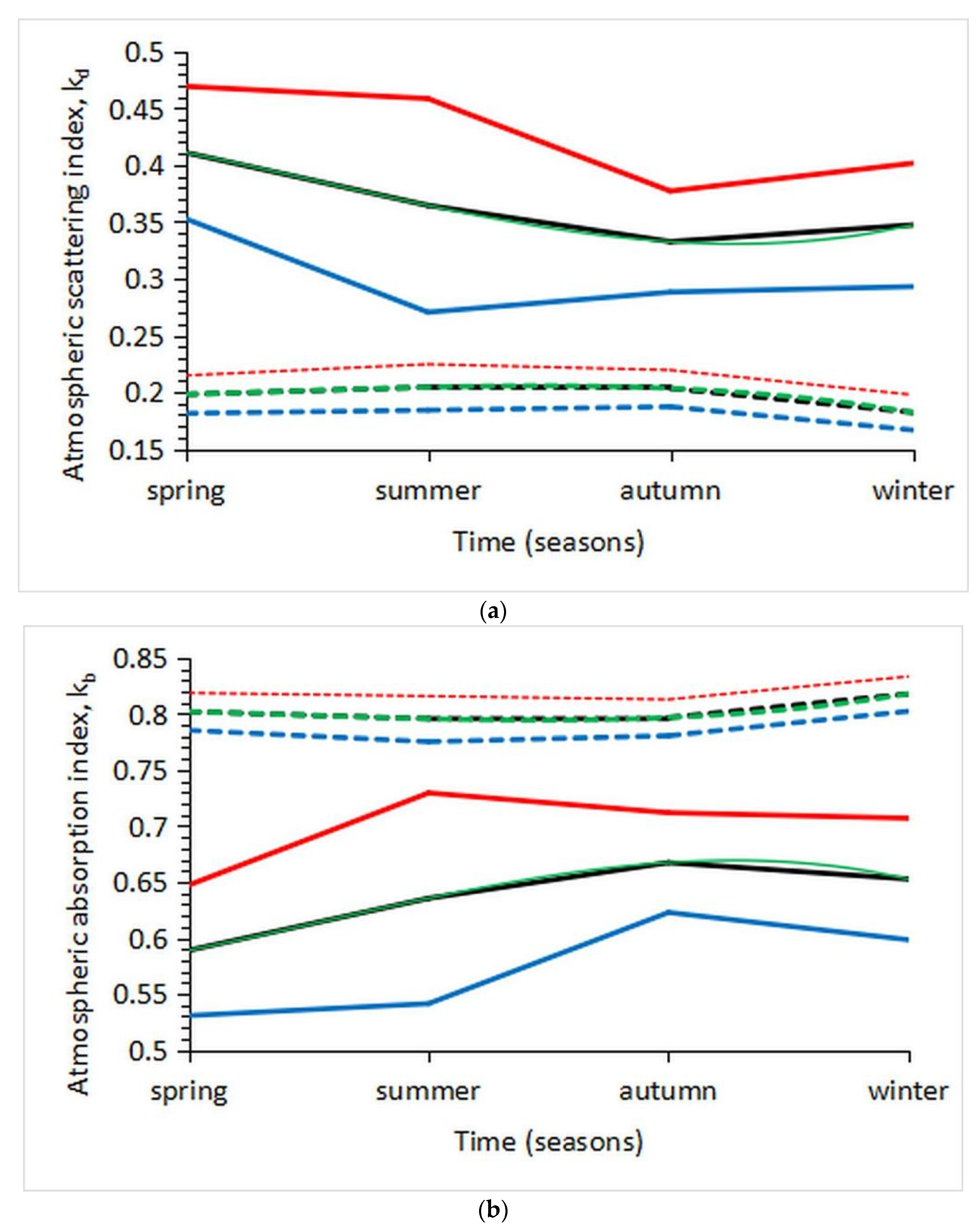
3.3. Seasonal Variation

Figure 5 shows the seasonal variation in G for all- (Figure 5a,c,e,g) and clear- (Figure 5b,d,f,h) sky conditions over Saudi Arabia for the study period (2013–2021). As was the case for the monthly values, the diagrams for SEZ-All (Figure 5a,b), SEZ-A (Figure 5c,d), SEZ-B (Figure 5e,f), and SEZ-C (Figure 5g,h) are shown. The black lines represent the seasonal mean G values, while the red and blue lines are the upper and lower limits of the ±1σ band, respectively, as in the case for the annual values. The green dotted curves are third-order polynomial fits to the mean curves. In all cases, the polynomial curves have an R² = 1, implying a perfect fit to the mean values (see

Table 3. Estimation of the seasonal mean values of G (Wm⁻²) and G_d (Wm⁻²),which are averages over the period 2013–2021 for all 43 sites in SEZ-All, or the sites belonging to the separate zones SEZ-A, SEZ-B, and SEZ-C. t is season (1 = spring, 4 = winter); statistical estimators for the model’s goodness-of-fit: RMSE (Wm⁻²), MAE (Wm⁻²), d, r, and R². All statistical results were computed with the MICROSOFT’s Excel 2021 functions.

Parameter	Regression Equation
Sky Type, SEZ	RMSE, MAE, d, r, R2
G	G = 28.7840t3 − 248.1000t2 + 565.2300t + 490.4100
clear, All	1.3607 × 10−6, 1.0186 × 10−5, 1.0000, 1.0000, 1.0000
Gd	Gd = 4.9610t3 − 48.6710t2 + 121.6400t + 88.6090
clear, All	3.3021 × 10−7, 2.6124 × 10−7, 1.0000, 1.0000, 1.0000
G	G = 19.3500t3 − 166.8700t2 + 393.9600t + 242.2300
all, All	2.5434 × 10−5, 2.2986 × 10−5, 1.0000, 1.0000, 1.0000
Gd	Gd = 8.5589t3 − 64.0850t2 + 118.3500t + 137.3600
all, All	5.0090 × 10−6, 3.5810 × 10−3, 1.0000, 1.0000, 1.0000
G	G = 19.5050t3 − 167.9200t2 + 373.7600t + 590.3300
clear, A	2.8695 × 10−5, 2.2848 × 10−5, 1.0000, 1.0000, 1.0000
Gd	Gd = 6.1111t3 − 56.9710t2 + 138.7600t + 84.9750
clear, A	5.4261 × 10−7, 3.8841 × 10−7, 1.0000, 1.0000, 1.0000
G	G = 2.1681t3 − 31.8100t2 + 83.6600t + 436.9200
all, A	5.5563 × 10−7, 3.6103 × 10−7, 1.0000, 1.0000, 1.0000
Gd	Gd = 16.4030t3 − 127.2800t2 + 270.5500t + 40.3750
all, A	1.2900 × 10−7, 1.1500 × 10−7, 1.0000, 1.0000, 1.0000
G	G = 34.9040t3 − 297.3200t2 + 679.4800t + 407.5700
clear, B	7.0687 × 10−7, 5.1574 × 10−7, 1.0000, 1.0000, 1.0000
Gd	Gd = 4.5135t3 − 45.7360t2 + 116.1200t + 87.0370
clear, B	1.4091 × 10−6, 1.0569 × 10−6, 1.0000, 1.0000, 1.0000
G	G = 33.0310t3 − 276.4600t2 + 651.8400t + 73.6310
all, B	6.2775 × 10−7, 4.1945 × 10−7, 1.0000, 1.0000, 1.0000
Gd	Gd = 1.2258t3 − 3.8163t2 − 30.6540t + 236.5500
all, B	1.2900 × 10−4, 1.2900 × 10−4, 1.0000, 1.0000, 1.0000
G	G = 25.6510t3 − 323.7000t2 + 550.2200t + 436.5100
clear, C	1.0768 × 10−6, 7.8333 × 10−7, 1.0000, 1.0000, 1.0000
Gd	Gd = −4.2375t3 + 20.3550t2 − 25.6560t + 144.52
clear, C	1.6750 × 10−6, 1.1708 × 10−6, 1.0000, 1.0000, 1.0000
G	G = 43.0670t3 − 349.3200t2 + 793.1900t + 9.9168
all, C	1.9157 × 10−6, 1.4250 × 10−5, 1.0000, 1.0000, 1.0000
Gd	Gd = −15.6520t3 + 120.2800t2 − 290.8400t + 359.9700
all, C	1.1200 × 10−7, 9.1700 × 10−8, 1.0000, 1.0000, 1.0000

for the regression equations and statistics). It is interesting to remark that in all SEZ cases, the peak seasonal values occur in the summer, as expected. Another interesting observation is the greater standard deviation band in the summer for the sites in SEZ-A (similar to the corresponding band in the SEZ-All case), for the reasons explained in Section 3.2. Conversely, this band is smaller in the winter, a finding that implies that the average weather patterns in this season are similar countrywide. The opposite occurred at the two sites in the SEZ-C zone. Here, the ±1σ band is wider in the winter than in the summer. This finding could be attributed to the differing environmental and/or terrain features [42], which could have had a decisive role in the solar radiation levels at the two sites. Similar behavior to G was found for the G_d solar component (not shown here). Table 3 includes the regression equations for G_d and G.

3.4. Specialized Analysis

Some further analysis of the data is described in this section. This is related to the following investigations:

(i)

the relationship between the direct horizontal irradiance, G_b, and the diffuse fraction, k_d;

(ii)

the dependence of the global, G, or diffuse, G_d, horizontal irradiance on the geographical latitude, φ, or the diffuse fraction, k_d;

(iii)

the dependence of the global, G, or diffuse, G_d, horizontal irradiance on the sites’ altitude, z; and

(iv)

the use of the diffuse fraction, k_d, and the direct-beam fraction, k_b, as atmospheric scattering and absorption indices, respectively, as proposed by [19,20]. In all investigations, no distinction was made regarding the SEZ to which the data points belonged, because Saudi Arabia was dealt here as unit.

(v)

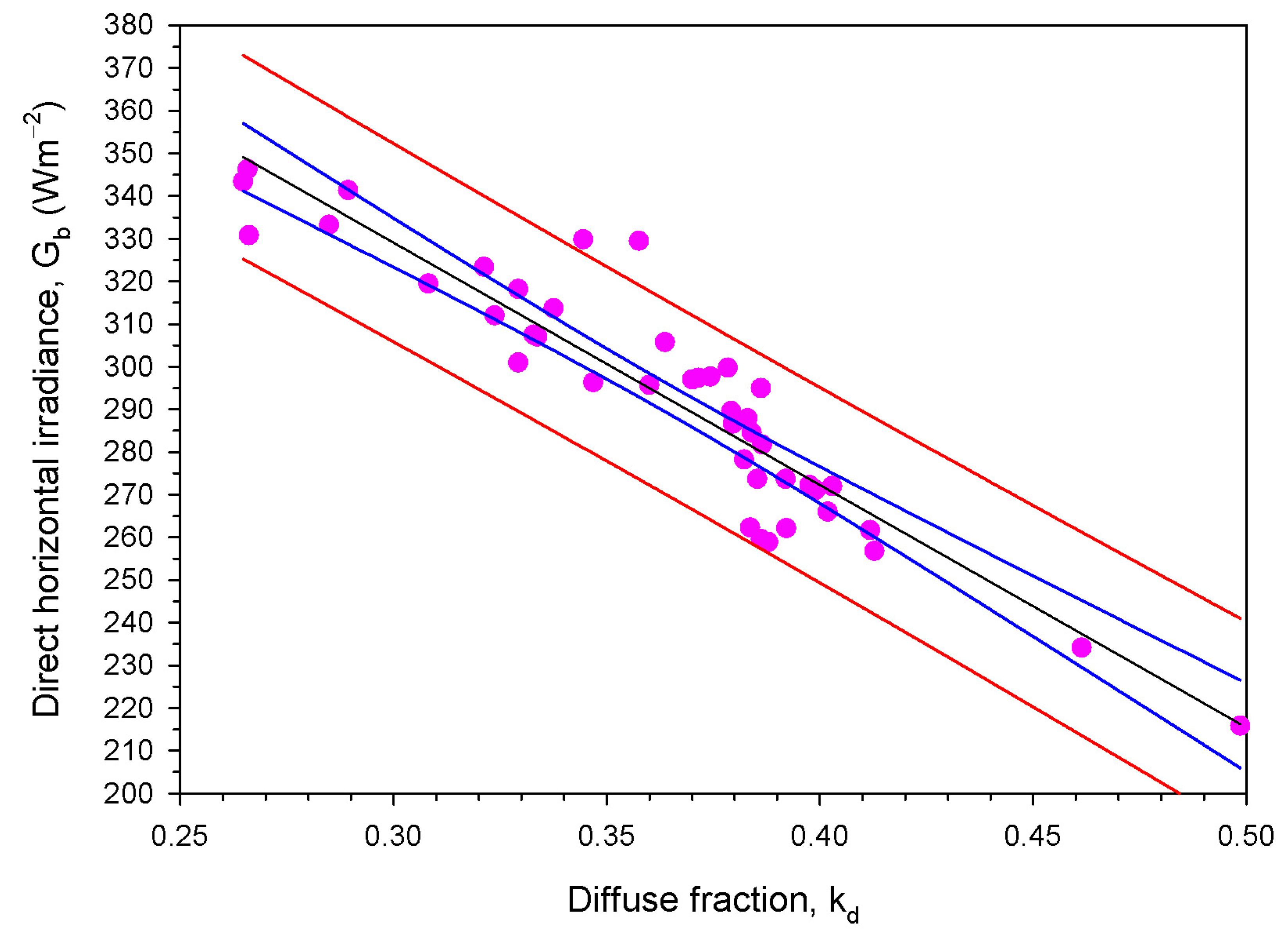
In order to find any relationship between G_b and k_d, a scatter plot of their annual mean values was prepared, which is presented in Figure 6. It is interesting to observe that almost all sites are included in the prediction interval, while very few are included in the confidence interval. The meaning of this observation is as follows: in the short term, the G_b–k_d data pairs are expressed by a linear relationship with a confidence interval much less than 95%, and, therefore, their relationship is not significant. Conversely, this relationship becomes significant at the 95% level in the long term (i.e., in the future under a changing global climate). Another interesting feature from Figure 6 is the negative linear dependence of G_b on k_d. If one assumes G is constant in the ratio G_d/G, then an increase in G_d (i.e., an increase in k_d) results in a decrease in G_b because of the linear relationship G = G_d + G_b or k_d = 1 − G_b/G (if both sides of the former equation are divided by G, the ratio G_d/G is replaced with k_d, and the equation is solved for k_d).

(vi)

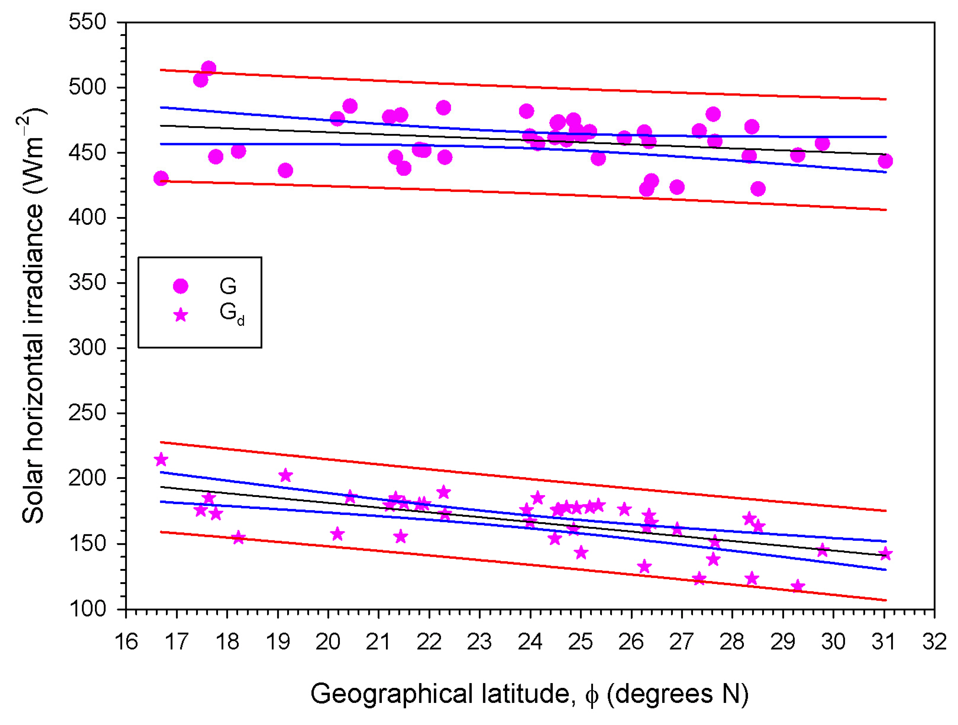
To investigate the dependence of G or G_d on k_d or on φ, Figure 7 and Figure 8 were derived. Figure 7 shows a plot of the annual mean G and G_d values versus the annual mean k_d ones, while Figure 8 presents a scatter plot of the annual mean G and G_d values versus φ for all 43 sites. Both scatter plots are fitted with linear regression lines from which the annual global or diffuse horizontal irradiance can be estimated with a known value for k_d or φ. The confidence and prediction intervals are shown and have the same meaning as those in Figure 6.

Almost none of the data points for either the G or the G_d solar component in Figure 7 lie outside its prediction band. This means that both the measured solar potential (in the form of G) and the atmospheric turbulence or atmospheric clearness, which includes cloudiness too (in the form of G_d), will be close to the future ones shown in the graph for the long term with 95% confidence. This will occur irrespective of the considered region of Saudi Arabia, because this is true for all SEZs, without exception, in the graph. A greater variability in the G values is observed, resulting in a broader prediction interval and a much lower R² than those for the G_d component. The interpretation of this outcome is that the atmospheric clearness over Saudi Arabia will be more unified and concentrated around its annual mean value, while the variability in the solar potential over the country will continue being as dispersed as it is today (probably because of small future climate changes and constant terrain features in the region). On the other hand, it is seen from the linear regression equations in the legend of Figure 7 that a 0.1 increase in k_d results in an as little as a 7.2 Wm⁻² decrease in G and an almost 40 Wm⁻² increase in G_d, on average. This observation can be interpreted by a greater effect of weather on the diffuse solar component than on the global one. Kambezidis [20] found a comparable decrease in G of 8.8 Wm⁻² for Greece on an annual basis.

The findings in Figure 8 are summarized in the following. The geographical latitude has little effect on the G or G_d levels across Saudi Arabia, because a 1° increase in φ has a very small effect on the G or G_d levels (decreases of 1.5 Wm⁻² in G and of 3.6 Wm⁻² in G_d, as seen from the linear regression equations in the legend of Figure 8). Additionally, the data points for G and G_d lie inside their prediction intervals, as in the case for their dependence on k_d, having a similar interpretation. Kambezidis [20] found a very similar decrease in G of 1.2 Wm⁻² for Greece on an annual basis.

(i)

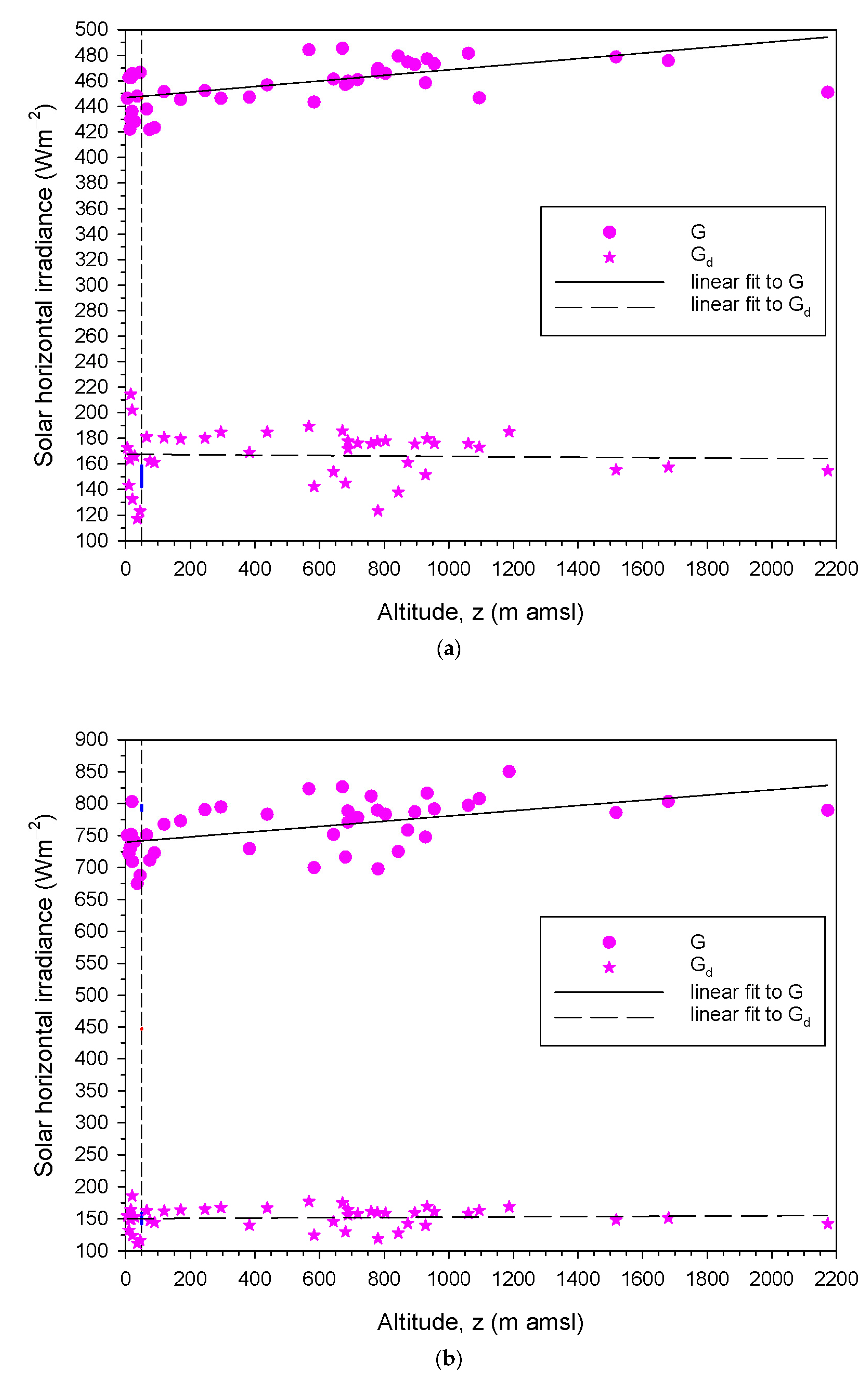
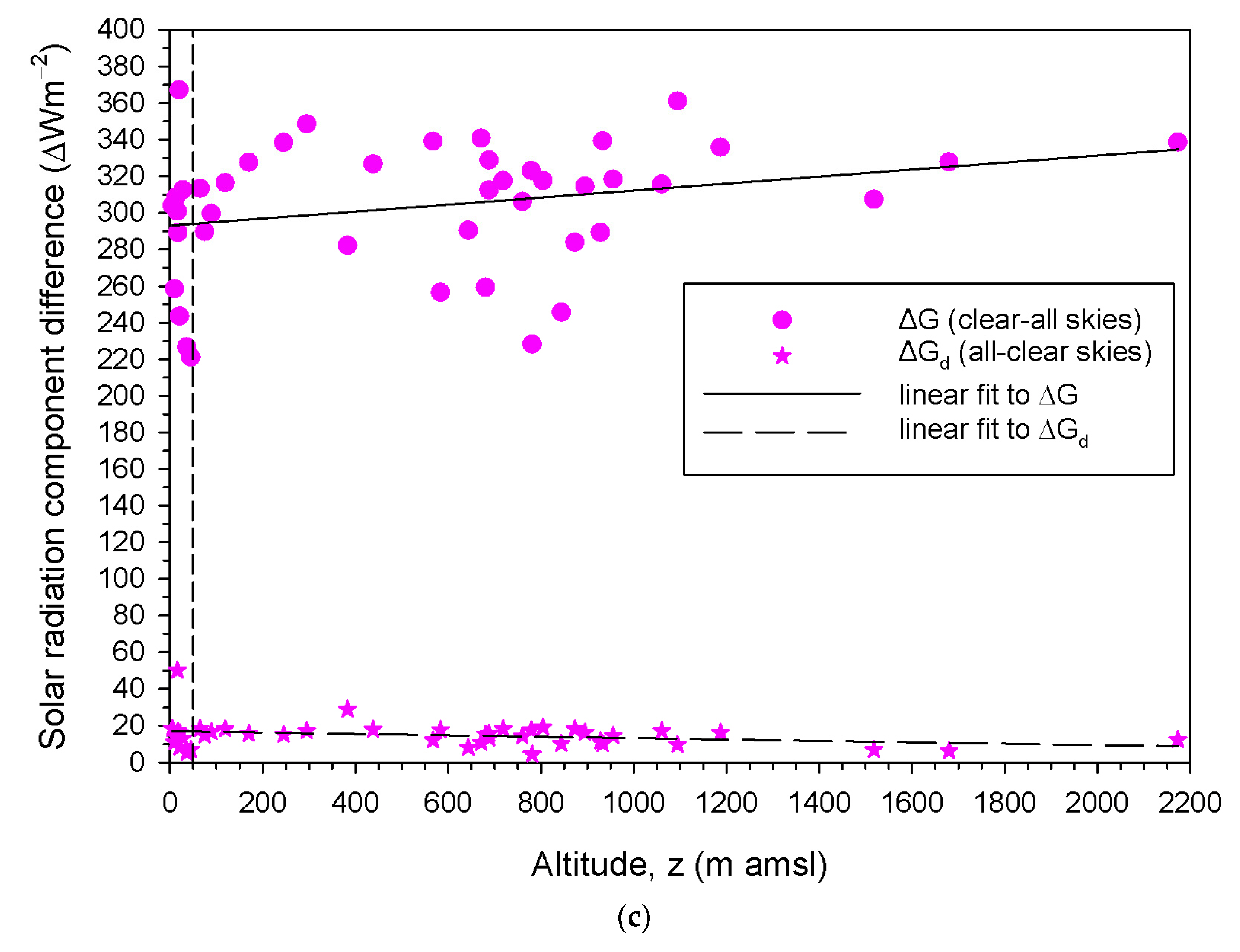
Figure 9a,b show the variation in both G and G_d levels versus the altitude of the sites in Saudi Arabia under all- and clear-sky conditions. It is shown that a variability in the levels of both solar components exists even at very low terrain elevations, i.e., below 50 m amsl (see the vertical dashed lines in Figure 9). In the entire altitude range of 0 m–2173 m amsl, the G levels vary between 422 Wm⁻² and 515 Wm⁻² (i.e., a difference of 93 Wm⁻²) under all skies and between 675 Wm⁻² and 850 Wm⁻² (i.e., a difference of 175 Wm⁻²) under clear skies, with average values at 459.38 Wm⁻² and 763.68 Wm⁻², respectively. These figures become 117 Wm⁻² to 214 Wm⁻² (i.e., a difference of 97 Wm⁻²) for all skies and 112 Wm⁻² to 186 Wm⁻² (i.e., a difference of 74 Wm⁻²) under clear skies for G_d, with average values at 166.59 Wm⁻² and 151.70 Wm⁻² for all- and clear-skies, respectively. The above results show that the annual G_d levels are dispersed in a much narrower band (74 Wm⁻²) than those for G (175 Wm⁻²) across all Saudi Arabia’s territories under clear skies. This implies a dispersion of atmospheric scattering in a narrow range (as a measure of G_d). One finding further related to the average values of G and G_d is that G is mostly composed of G_b (direct horizontal irradiance), because the values in the differences $\overline{{\mathrm{G}}_{\mathrm{b}}}=\overline{\mathrm{G}}-\overline{{\mathrm{G}}_{\mathrm{d}}}$ (the over-bar indicates averaging) are high: 292.79 Wm⁻² and 611.98 Wm⁻², for all- and clear-sky conditions, respectively. This result is also confirmed by the almost-neutral (zero-sloped) linear fits to the (G_d, z) data pairs, especially in Figure 9a,b. In all cases, the wide scatter of the data points is shown by the low R² values. Moreover, according to Kambezidis [19,20], G_b is a measure of atmospheric absorption and is used below as such. Figure 9c is a combination of Figure 9a,b in the sense that it shows the (positive) differences in ΔG = G_{clear skies} − G_{all skies} and ΔG_d = G_{d,all skies} − G_{d,clear skies}. These ΔG values show a broad variability in the altitude range 0 m–1000 m, a finding that may be attributed to the variations in the weather patterns, which affect solar radiation on this altitude scale. Conversely, the dispersion of the ΔG_d values is very low at all altitudes, a finding that implies little or even a negligible effect of weather on atmospheric scattering (expressed as a measure of G_d). The high/low dispersion of the ΔG/ΔG_d values is depicted in the corresponding lower/higher R² values.

(ii)

Kambezidis [20] examined the atmospheric scattering in a study on Greece in terms of the diffuse fraction (or else atmospheric scattering index), k_d. In the same way, the absorption of solar radiation can be expressed by the direct-beam fraction (or the atmospheric absorption index), k_b = G_b/G. By dividing both sides of the basic equation G = G_d + G_b by G, we obtain the expression 1 = k_d + k_b, if G_d/G and G_b/G are replaced with k_d and k_b, respectively [20]. Practically, this theoretical result is experimentally confirmed by the summation of the linear regression equations for the same solar radiation component side-by-side (see legend in Figure 10). This equation shows that the scattering and absorption effects (if reflections in the atmosphere are omitted) sum up to one (i.e., to the total extinction of solar rays). To demonstrate this, Figure 10 show the annual mean values of k_d and k_b over the 43 sites in Saudi Arabia as function of φ under all (Figure 10a) and clear (Figure 10b) skies. It is clearly shown that the absorption mechanism is always stronger over Saudi Arabia, i.e., k_b ≈ 2k_d and k_b ≈ 4k_d, under all- and clear-sky conditions, respectively (same conclusion was obtained for Greece [20]). On the other hand, it is quite interesting to observe that either atmospheric mechanism is almost constant over all of Saudi Arabia under clear-sky conditions (the same conclusion was reached for Greece [20]). This observation implies a uniformity of the scattering and absorbing particles over the country because, in fair weather, the extinction of solar light is only due to the atmospheric constituents (excluding reflections from the ground). The extinction comes from the atmospheric particles that scatter (nitrogen, oxygen, and desert dust) and/or absorb (carbon dioxide, water vapor, and ozone) solar light. Under all-sky conditions (Figure 10a), the scatterers/absorbers seem to have an increasing/decreasing effect with increasing geographical latitude. This occurs because the extra particles in the atmosphere in this case are the clouds that unevenly scatter solar light. Therefore, as φ increases from 16° N to 32° N, so does the probability of cloudiness (in terms of cloud cover and cloud texture). These additional particles in the atmosphere cause increased scattering of solar radiation, and, thus, decreased absorption because of the basic equation k_d + k_b = 1. The verification of this equation is easy if the values of k_d and k_b for any 16° < φ < 32° are replaced with the corresponding expressions of the best-fit lines shown in the legend of Figure 10a,b. According to the above discussion, the bigger scatter of the k_d or k_b data points under all-sky conditions (Figure 10a) is due to the presence of clouds. Moreover, the theoretical expression of k_d + k_b = 1 is shown in Figure 10c, which presents a graph of the annual mean values of k_b versus k_d; it is shown that all data points lie on the same line, which is expressed by the linear fit of k_b = 1 − k_d.

Bai and Zong [43], in an effort to develop a solar radiation model to estimate G for the Qianyanzhou area, China, as a sum of absorbing and scattering losses in the atmosphere, observed that: (i) the absorbing losses (expressed as percentage of their R_LA factor for k_d ≥ 0.80 under all-sky conditions and k_d < 0.80 under clear-sky conditions; Table 3 in their publication) were higher in spring and winter (in agreement with the solid black line in Figure 11b in the present study, showing lower k_b values in all-sky conditions, but in relative disagreement with the dashed black line in Figure 11b showing higher values in clear skies); (ii) the scattering losses (expressed as percentage of their R_LS factor for all-sky conditions; Table 3 in their publication) were higher in summer and autumn (in agreement with the solid line in Figure 11a in the present study showing lower k_d values) and higher in spring and winter under clear skies (in comparison with the dashed black line in Figure 11a in the present study). The slight disagreement between the findings in [43] and those of the present study for clear skies may be due to year-round variations in atmospheric aerosols (concentration and type) between China and Saudi Arabia.

Kafka and Miller [36] introduced the G_d/G_b ratio, which is the atmospheric extinction index, k_e, in the present study. This index ranges between zero and one; in these two extremes, it refers to the dominance (when G_d = 0) and equality (if G_d = G_b) of G_b. Because both solar radiation components take part in the expression of k_e, they denote the contribution of the scattering (by the G_d component) and absorption (by the G_b component) mechanisms in the atmosphere, and thereby contribute to the meaning of k_e as an atmospheric extinction index. The k_e index is useful for various applications (e.g., PV installation) because it denotes the significant fractional amount of each solar component to solar harvesting [36]. Figure 11c shows that spring and summer are the two seasons with greater solar potential availability under all types of weather (black solid line in Figure 11c), while in clear-sky conditions, the solar harvesting is almost constant throughout the year but lower than in all-weather situations (dashed black line in Figure 11c).

3.5. Annual Solar Maps

This section is devoted to the presentation of the distribution of the annual mean values of the five examined parameters (G, G_d, k_d, k_b, and k_e) over Saudi Arabia. The annual values for each parameter at all 43 sites were inserted in the ESRI’s ArcGIS Desktop 10.7.0.10450 software, and the kriging geospatial tool was invoked in order to calculate and extend all the values of the parameter in question within the territory of Saudi Arabia. The output of this process was the derivation of 10 maps (2 for each parameter under all- and clear-sky conditions). These maps are shown in Figure 12a–j. No application of the SEZs was made here, because our interest was focused on the distribution of the parameters across the country regardless of energy zone.

The distribution of the diffuse horizontal irradiance throughout Saudi Arabia is shown in Figure 12c,d under all- and clear-sky conditions, respectively. The pattern looks the same in both cases; this finding implies that G_d is distributed the same across the country in any type of weather, the only difference being the intensity levels under all and clear skies, as anticipated. Moreover, the G_d pattern seems to prevail and affect that of the G component under clear skies (Figure 12b). This was not the case for G under all skies, as clouds (in other words, the weather patterns) modulate the G levels (Figure 12a). Nevertheless, both solar components showed low values in the north and higher ones in the south of Saudi Arabia; the high values geographically coincide with the Rub Al-Khali desert, which extends along the southern border of Saudi Arabia to Yemen and Oman with dimensions 1000 km × 500 km. This high solar potential is located in a harsh environment; however, the exploitation of the available high solar energy because of the large amount of sunshine hours (i.e., clear weather) in this area constitutes a challenge [44]. Agreement exists between the annual map for G over Saudi Arabia (Figure 12a in the present work) and that derived in a study by Farahat et al. [45] (their Figure 8a). Nevertheless, the annual G map for Saudi Arabia in [29] (Figure on page 39) shows a consistent color (i.e., same value) for the solar component; therefore, a complete disagreement exists with the results of the present work. On the other hand, AlYaya and Irfan [28] reported monthly maps of only G_bn; therefore, no comparison can be made with our results.

The pattern of the atmospheric scattering index, k_d, (see Figure 12e,f) follows that for G_d. This observation drives the conclusion that the G_d component is dominant over G (recall that k_d = G_d/G). The same conclusion for the dominance of G_d over G was drawn in the preceding paragraph, too. Now, considering k_d as a scattering index, it was found that lower values prevail in the northern part of the country in agreement with those for G.

As far as k_b is concerned, its pattern is quite the opposite that of k_d (see Figure 12g,h) because of the basic equation k_b = 1 − k_d. The explanation for this result lies in the higher air pollutant (absorber) concentration over the northern region of Saudi Arabia. These pollutants are either dust particles from eastern Egypt or northwestern Saudi Arabia [46] or CO₂ aerosols from industry and transportation [47].

The last two panels in Figure 12 contain significant information. According to [36], the k_e index denotes the fractional amount of each solar component that significantly contributes to solar harvesting. In other words, a value of k_e = G_d/G_b = 0.7 means that 70% of the solar radiation incident on a solar system for energy production comes from diffuse radiation and only 30% from direct-beam radiation. Therefore, in areas with higher k_e values, the G_d component contributes more than G_b and vice versa. Considering a PV system installation, the investor should choose a location within Saudi Arabia depending on their cost–benefit analysis; at locations with low k_e values, the PV system will work efficiently under clear or almost-clear weather because of the more abundant direct-beam radiation. Conversely, in areas with high k_e values all-year round, one should design a PV system with more solar panels (and therefore higher cost) because of the abundant diffuse radiation.

It can be seen from Figure 12b,d,f,h,j that the country may be divided into two parts, a northern part with higher G, G_d, k_d, and k_e and lower k_b; and a southern part with higher k_b and lower G, G_d, k_d, and k_e values. The dividing line is located at φ ≈ 25° N.

4. Discussion and Conclusions

The present work studied the solar radiation climate of Saudi Arabia, using measurements of solar radiation data at 43 sites available from the K.A.CARE research program of Saudi Arabia. This work is the first in Saudi Arabia studying the solar radiation climate of the country and among the few in the international literature. The knowledge of the solar climate in a region or of a country is significant, as it provides information about the solar availability and the solar radiation levels expected; to a certain extent, it describes the climate of the area, because solar radiation is one of the most important parameters constituting the climate. The analysis in the present study was focused on the three solar radiation components (primarily, global and diffuse horizontal irradiances; secondarily, direct horizontal irradiance) for 43 sites in Saudi Arabia. We used the diffuse fraction, k_d, (or cloudiness index [48]), and the absorption index, k_b. Furthermore, we used the ratio k_e = G_d/G_b for the first time in Saudi Arabia, which was given the name “atmospheric extinction index”.

The diffuse fraction (atmospheric scattering index) shows the weight of the diffusively scattered solar radiation by atmospheric molecules (in clear skies) and by atmospheric aerosols (e.g., desert dust) and clouds combined (in all skies) over the received global solar radiation on the surface of the Earth. In other words, k_d reflects the attenuation of solar radiation by scattering alone in the atmosphere. The direct-beam fraction (atmospheric absorption index) conveys information about the weight of the attenuated (absorbed) direct solar radiation by atmospheric molecules (in clear-sky conditions) or attenuated by atmospheric aerosols (e.g., air pollutants) and clouds (in all-sky conditions) to the global solar irradiance received on the surface of the Earth. The k_e factor (atmospheric extinction index) gives information about the percentage contribution of both the G_d and G_b solar radiation components to solar applications over the country and, more specifically, to PV installations.

In view of the above, the following conclusions could be drawn:

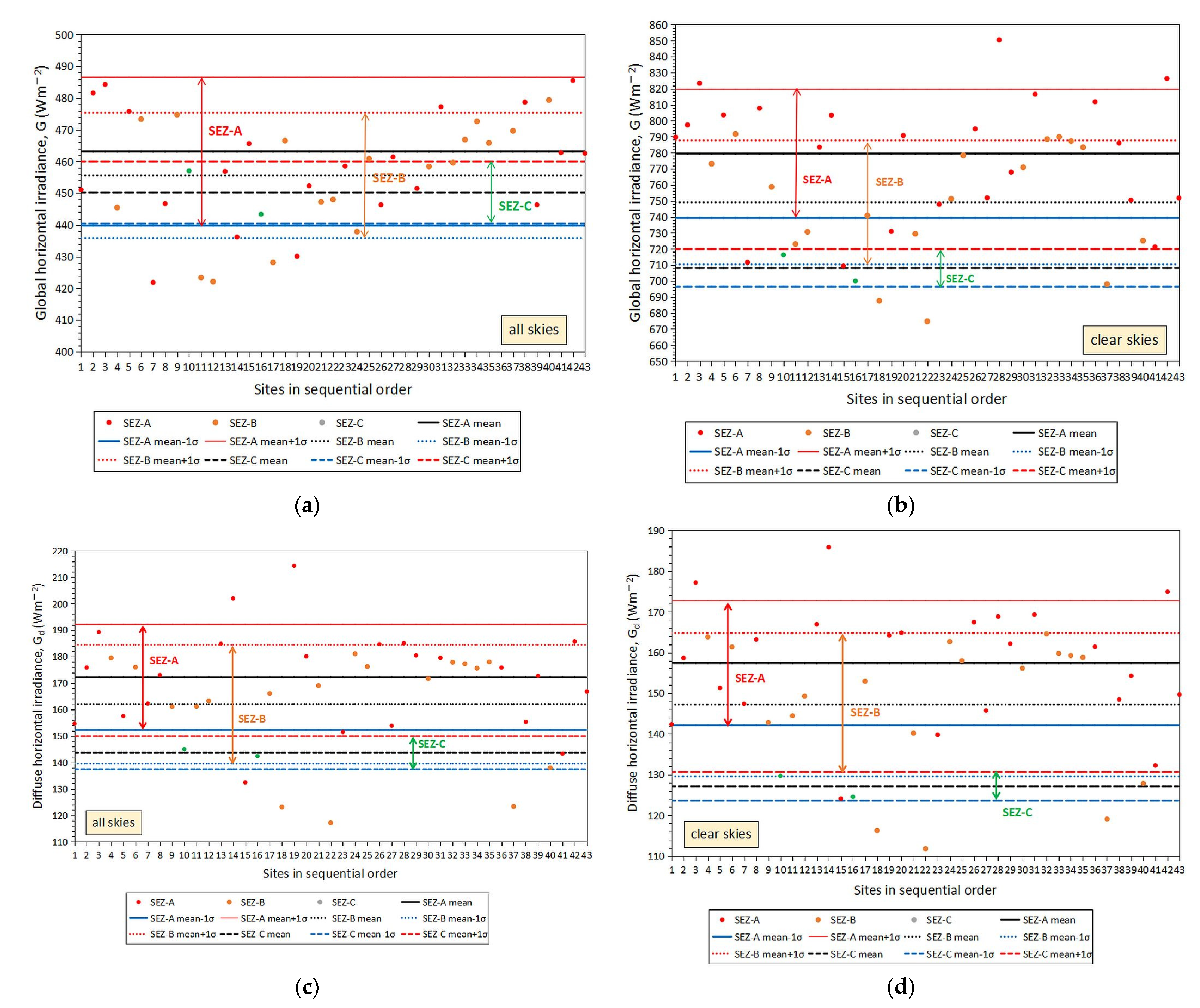
• Under all-sky conditions, the annual mean G radiation values were found to decrease from SEZ-A to SEZ-C (463 Wm⁻², 456 Wm⁻², and 450 Wm⁻², respectively). Additionally, the ±1σ band for the SEZ-A and SEZ-B zones was estimated to be greater than that for SEZ-C; this finding was attributed to the low (just two) number of sites in the SEZ-C zone. The annual G average, regardless of energy zones, was found to be between those for SEZ-A and SEZ-B (i.e., 459 Wm⁻²). The intra-annual mean G variation reached a maximum in the summer (June), particularly for SEZ-All, SEZ-A, and SEZ-B, and in July for the SEZ-C zone. Sixth-order regression equations were derived for estimating G as a function of the month of the year for all three SEZs and SEZ-All. At the seasonal scale, the G values peaked in the summer and dropped in winter for all SEZs, as expected. Again, third-order polynomial fits were derived to estimate the G value as a function of the season. For the annual, seasonal, and intra-annual G_d variations, they were shown to have a very similar behavior to that of G, and, for this reason, they were not included in the Results section. The annual mean values were estimated at 172 Wm⁻², 162 Wm⁻², 144 Wm⁻², and 166 Wm⁻² for SEZ-A, SEZ-B, SEZ-C, and SEZ-All, respectively.
• Under clear skies, the annual mean G radiation values were found to decrease from SEZ-A to SEZ-C (779 Wm⁻², 749 Wm⁻², and 708 Wm⁻², respectively), as much as in the case under all-sky conditions. Additionally, the ±1σ band for the SEZ-A and SEZ-B zones was estimated to be greater than that for SEZ-C. The annual G average regardless of energy zone was found to be between those for SEZ-A and SEZ-B (i.e., 763 Wm⁻²). The intra-annual mean G variation showed a maximum in June for SEZ-All, and a broad maximum from April to September in the SEZ-A, SEZ-B, and SEZ-C energy zones. Sixth-order regression equations were also derived for estimating G as a function of the month of the year for all three SEZs and SEZ-All. At the seasonal scale, the G values showed an exactly similar behavior to that for the seasonal G variation. Again, third-order polynomial fits were derived to estimate the G value as a function of the season. For the annual, seasonal, and intra-annual G_d variations, they were shown to have very similar behaviors to that for G in the case of all-sky conditions; for this reason, they were not included in the Results section. Nevertheless, the annual mean values were estimated at 157 Wm⁻², 147 Wm⁻², 127 Wm⁻², and 152 Wm⁻² for SEZ-A, SEZ-B, SEZ-C, and SEZ-All, respectively.
• A further specialized analysis was conducted for all the investigated parameters in this study (annual mean values of G, G_d, G_b, k_d, k_b, and k_e) regardless of the solar energy zone. A declining expression was found for G_b vs. k_d for all sites in Saudi Arabia under any type of sky condition. As G_d increased in the G_d/G = k_d ratio (assuming a constant value of G), G_b decreased because of the expression G_constant = G_d + G_b. Another outcome was the almost negligible effect of φ on the G and G_d levels across Saudi Arabia under all-sky conditions. This was also the case for the G_d levels as a function of z under any type of sky; conversely, the relationship of G vs. z had an increasing trend under both all and clear skies. A side product of this analysis was the much lower dispersion of the G_d values in comparison with that of the G values for all types of weather.

A further speculation from the specialized analysis concerned the k_d, k_b, and k_e indices, which were treated as atmospheric scattering, absorption, and extinction indices, respectively. We found an increasing/decreasing behavior of k_d/k_b as a function of φ under all skies; to the contrary, this relationship proved to be nearly neutral (no increase or decrease) for clear skies, implying a rather uniform dispersion of scatterers/absorbers over Saudi Arabia year-round. Regarding their seasonal variation, low values were found for k_d and k_e and higher values for k_b in autumn under all-sky conditions, while the situation reversed for clear skies. The findings for the k_e index were important: they are related to the solar availability in Saudi Arabia because this index shows the contribution of the G_d and G_b components to solar harvesting.

The last item in the analysis was the derivation of annual maps for the parameters under investigation for all and clear skies across Saudi Arabia. These maps were generated via the ESRI’s ArcGIS Desktop 10.7.0.10450 geospatial software by using the kriging method to extend the annual values of the parameters estimated at the 43 sites to all the territories in the country. The patterns in all cases (all five parameters under both types of sky) were found to be similar, i.e., higher values in the southern part of Saudi Arabia. The exception was the k_b index, the pattern of which was the reverse of that of the other four. The two distinct patterns (higher/lower values) could be recognized by a dividing line at the latitude of φ ≈ 25° N.

Because of the high solar radiation levels, especially in the southern region of Saudi Arabia, the country has decided to implement the Saudi Arabia 2030 Vision program, which describes how the country will gradually shift from fossil fuels to renewable (mostly solar) energy in the near future [49].

References

1. Giesen, R.H.; van den Broeke, M.R.; Oerlemans, J.; Andreassen, L.M. Surface Energy Balance in the Ablation Zone of Midtdalsbreen, a Glacier in Southern Norway: Interannual Variability and the Effect of Clouds. J. Geophys. Res. 2008, 113, D21111. [Google Scholar] [CrossRef]
2. Asaf, D.; Rotenberg, E.; Tatarinov, F.; Dicken, U.; Montzka, S.A.; Yakir, D. Ecosystem Photosynthesis Inferred from Measurements of Carbonyl Sulphide Flux. Nat. Geosci. 2013, 6, 186–190. [Google Scholar] [CrossRef]
3. Bojinski, S.; Verstraete, M.; Peterson, T.C.; Richter, C.; Simmons, A.; Zemp, M. The Concept of Essential Climate Variables in Support of Climate Research, Applications, and Policy. Bull. Am. Meteorol. Soc. 2014, 95, 1431–1443. [Google Scholar] [CrossRef] [Green Version]
4. Kambezidis, H.D. The Solar Resource. Compr. Renew. Energy 2012, 3, 27–84. [Google Scholar] [CrossRef]
5. Kambezidis, H.D. The Solar Radiation Climate of Athens: Variations and Tendencies in the Period 1992–2017, the Brightening Era. Sol. Energy 2018, 173, 328–347. [Google Scholar] [CrossRef]
6. Forster, P.M. Inference of Climate Sensitivity from Analysis of Earth’s Energy Budget. Annu. Rev. Earth Planet. Sci. 2016, 44, 85–106. [Google Scholar] [CrossRef]
7. Haywood, J.; Boucher, O. Estimates of the Direct and Indirect Radiative Forcing Due to Tropospheric Aerosols: A Review. Rev. Geophys. 2000, 38, 513–543. [Google Scholar] [CrossRef]
8. Puetz, S.J.; Prokoph, A.; Borchardt, G. Evaluating Alternatives to the Milankovitch Theory. J. Stat. Plan. Inference 2016, 170, 158–165. [Google Scholar] [CrossRef] [Green Version]
9. Madhlopa, A. Solar Radiation Climate in Malawi. Sol. Energy 2006, 80, 1055–1057. [Google Scholar] [CrossRef]
10. Jiménez, J.I. Solar Radiation Statistic in Barcelona, Spain. Sol. Energy 1981, 27, 271–282. [Google Scholar] [CrossRef]
11. Dissing, D.; Wendler, G. Solar Radiation Climatology of Alaska. Theor. Appl. Climatol. 1998, 61, 161–175. [Google Scholar] [CrossRef]
12. Petrenz, N.; Sommer, M.; Berger, F.H. Long-Time Global Radiation for Central Europe Derived from ISCCP Dx Data. Atmos. Chem. Phys. 2007, 7, 5021–5032. [Google Scholar] [CrossRef] [Green Version]
13. Nottrott, A.; Kleissl, J. Validation of the NSRDB-SUNY Global Horizontal Irradiance in California. Sol. Energy 2010, 84, 1816–1827. [Google Scholar] [CrossRef]
14. Persson, T. Solar Radiation Climate in Sweden. Phys. Chem. Earth 1999, 24, 275–279. [Google Scholar] [CrossRef]
15. Exell, R.H.B. The Solar Radiation Climate of Thailand. Sol. Energy 1976, 18, 349–354. [Google Scholar] [CrossRef]
16. Diabaté, L.; Blanc, P.; Wald, L. Solar Radiation Climate in Africa. Sol. Energy 2004, 76, 733–744. [Google Scholar] [CrossRef] [Green Version]
17. Kambezidis, H. A Look at the Solar Radiation Climate in Athens during the Brightening Period. Sci. Trends 2018. [Google Scholar] [CrossRef]
18. Kambezidis, H.D. The Daylight Climate of Athens: Variations and Tendencies in the Period 1992–2017, the Brightening Era. Light. Res. Technol. 2020, 52, 202–232. [Google Scholar] [CrossRef]
19. Kambezidis, H.D. The Sky-Status Climatology of Greece: Emphasis on Sunshine Duration and Atmospheric Scattering. Appl. Sci. 2022, 12, 7969. [Google Scholar] [CrossRef]
20. Kambezidis, H.D. The Solar Radiation Climate of Greece. Climate 2021, 9, 183. [Google Scholar] [CrossRef]
21. Tarawneh, Q.Y.; Chowdhury, S. Trends of Climate Change in Saudi Arabia: Implications on Water Resources. Climate 2018, 6, 8. [Google Scholar] [CrossRef] [Green Version]
22. Marzo, A.; Trigo, M.; Alonso-Montesinos, J.; Martínez-Durbán, M.; López, G.; Ferrada, P.; Fuentealba, E.; Cortés, M.; Batlles, F.J. Daily Global Solar Radiation Estimation in Desert Areas Using Daily Extreme Temperatures and Extraterrestrial Radiation. Renew. Energy 2017, 113, 303–311. [Google Scholar] [CrossRef]
23. Behar, O.; Sbarbaro, D.; Marzo, A.; Gonzalez, M.T.; Vidal, E.F.; Moran, L. Critical Analysis and Performance Comparison of Thirty-Eight (38) Clear-Sky Direct Irradiance Models under the Climate of Chilean Atacama Desert. Renew. Energy 2020, 153, 49–60. [Google Scholar] [CrossRef]
24. Gairaa, K.; Chellali, F.; Benkaciali, S.; Messlem, Y.; Abdallah, K. Daily Global Solar Radiation Forecasting over a Desert Area Using NAR Neural Networks. In Proceedings of the International Conference on Renewable Energy Research and Applications (ICRERA), Palermo, Italy, 22–25 November 2015; pp. 567–571. [Google Scholar]
25. Bahel, V.; Srinivasan, R.; Bakhsh, H. Solar Radiation for Dhahran, Saudi Arabia. Energy 1986, 11, 985–989. [Google Scholar] [CrossRef]
26. Aksakal, A.; Rehman, S. Global Solar Radiation in Northeastern Saudi Arabia. Renew. Energy 1999, 17, 461–472. [Google Scholar] [CrossRef]
27. Sahin, A.Z.; Aksakal, A.; Kahraman, R. Solar Radiation Availability in the Northeastern Region of Saudi Arabia. Energy Sources 2000, 22, 859–864. [Google Scholar] [CrossRef]
28. AlYahya, S.; Irfan, M.A. Analysis from the New Solar Radiation Atlas for Saudi Arabia. Sol. Energy 2016, 130, 116–127. [Google Scholar] [CrossRef]
29. National Renewable Energy Laboratory. Kingdom of Saudi Arabia: Solar Radiation Atlas. 1998. Available online: https://digital.library.unt.edu/ark:/67531/metadc690351 (accessed on 1 November 2022).
30. Myers, D.R.; Wilcox, S.M.; Marion, W.F.; Al-Abbadi, N.M.; bin Mahfoodh, M.; Al-Otaibi, M. Final Report for Annex II, Assessment of Solar Radiation Resources in Saudi Arabia 1998–2000. 2002. Available online: www.ntis.gov/ordering.htm (accessed on 1 November 2022).
31. Alnaser, W.E.; Eliagoubi, B.; Al-Kalak, A.; Trabelsi, H.; Al-Maalej, M.; El-Sayed, H.M.; Alloush, M. First Solar Radiation Atlas for the Arab World. Renew. Energy 2004, 29, 1085–1107. [Google Scholar] [CrossRef]
32. ESMAP. Global Solar Atlas 2.0; ESMAP: Washington, DC, USA, 2019; Available online: www.solargis.com (accessed on 1 November 2022).
33. Dervishi, S.; Mahdavi, A. Computing Diffuse Fraction of Global Horizontal Solar Radiation: A Model Comparison. Sol. Energy 2012, 86, 1796–1802. [Google Scholar] [CrossRef] [Green Version]
34. Babatunde, A.; Vincent, O.O. Estimation of Hourly Clearness Index and Diffuse Fraction Over Coastal and Sahel Regions of Nigeria Using NCEP/NCAR Satellite Data. J. Energy Res. Rev. 2021, 7, 1–18. [Google Scholar] [CrossRef]
35. Bailek, N.; Bouchouicha, K.; El-Shimy, M.; Slimani, A.; Chang, K.-C.; Djaafari, A. Improved Mathematical Modeling of the Hourly Solar Diffuse Fraction (HSDF) -Adrar, Algeria Case Study. Int. J. Math. Anal. Appl. 2017, 4, 8–12. [Google Scholar]
36. Kafka, J.L.; Miller, M.A. A Climatology of Solar Irradiance and Its Controls across the United States: Implications for Solar Panel Orientation. Renew. Energy 2019, 135, 897–907. [Google Scholar] [CrossRef]
37. K.A.CARE. Renewable Resource Atlas. Available online: https://rratlas.kacare.gov.sa (accessed on 20 March 2022).
38. Albalawi, H.; Balasubramaniam, K.; Makram, E. Secure Operation and Optimal Generation Scheduling Considering Battery Life for an Isolated Northwest Grid of Saudi Arabia. J. Power Energy Eng. 2017, 5, 41–62. [Google Scholar] [CrossRef] [Green Version]
39. Kambezidis, H.D.; Kampezidou, S.I.; Kampezidou, D. Mathematical Determination of the Upper and Lower Limits of the Diffuse Fraction at Any Site. Appl. Sci. 2021, 11, 8654. [Google Scholar] [CrossRef]
40. Farahat, A.; Kambezidis, H.D.; Almazroui, M.; Ramadan, E. Solar Potential in Saudi Arabia for Southward-Inclined Flat-Plate Surfaces. Appl. Sci. 2021, 11, 4101. [Google Scholar] [CrossRef]
41. Willmott, C.J. On the Validation of Models. Phys. Geogr. 1981, 2, 184–194. [Google Scholar] [CrossRef]
42. Almazroui, M. Simulation of Present and Future Climate of Saudi Arabia Using a Regional Climate Model (PRECIS). Int. J. Climatol. 2013, 33, 2247–2259. [Google Scholar] [CrossRef]
43. Bai, J.; Zong, X. Global Solar Radiation Transfer and Its Loss in the Atmosphere. Appl. Sci. 2021, 11, 2651. [Google Scholar] [CrossRef]
44. Mohandes, M.A.; Rehman, S. Estimation of Sunshine Duration in Saudi Arabia. J. Renew. Sustain. Energy 2013, 5, 033128. [Google Scholar] [CrossRef]
45. Farahat, A.; Kambezidis, H.D.; Almazroui, M.; al Otaibi, M. Solar Potential in Saudi Arabia for Inclined Flat-Plate Surfaces of Constant Tilt Tracking the Sun. Appl. Sci. 2021, 11, 7105. [Google Scholar] [CrossRef]
46. Farahat, A.; El-Askary, H.; Al-Shaibani, A. Study of Aerosols’ Characteristics and Dynamics over the Kingdom of Saudi Arabia Using a Multisensor Approach Combined with Ground Observations. Adv. Meteorol. 2015, 2015, 247531. [Google Scholar] [CrossRef] [Green Version]
47. Farahat, A. Air Pollution in the Arabian Peninsula (Saudi Arabia, the United Arab Emirates, Kuwait, Qatar, Bahrain, and Oman): Causes, Effects, and Aerosol Categorization. Arab. J. Geosci. 2016, 9, 196. [Google Scholar] [CrossRef]
48. Soneye, O.O. Evaluation of Clearness Index and Cloudiness Index Using Measured Global Solar Radiation Data: A Case Study for a Tropical Climatic Region of Nigeria. Atmosfera 2021, 34, 25–39. [Google Scholar] [CrossRef]
49. Hepbasli, A.; Alsuhaibani, Z. A Key Review on Present Status and Future Directions of Solar Energy Studies and Applications in Saudi Arabia. Renew. Sustain. Energy Rev. 2011, 15, 5021–5050. [Google Scholar] [CrossRef]
Figure 2. Annual mean (a) G and (c) Gd values for all-sky and annual mean (b) G and (d) Gd values for clear-sky conditions over Saudi Arabia in the period 2013–2021. The data points are colored according to the SEZ to which they belong (Table 1 and Figure 1). The ±1σ range around the mean value for each SEZ is shown by a vertical double-arrow line in the same color as the SEZ. All plots were derived with the MICROSOFT’s Excel 2021 utilities.
Climate 11 00075 g002
Figure 3. Annual mean (a) G and (c) Gd values for all-sky conditions, and annual mean (b) G and (d) Gd values for clear-sky conditions over Saudi Arabia in the period 2013–2021. The 3 colored bars indicate the average annual values of the solar components for the corresponding SEZ over all sites to which they belong; the black bar includes all sites irrespective of their SEZ. The error bars represent the ±1σ (±1 standard deviations) around the means. The numbers on the x-axis have no real meaning. All plots were derived with the SYSTAT’s SigmaPlot 14.0.0.124 graphing software.
Climate 11 00075 g003
Figure 4. Monthly mean G values under all—(left panels) and clear—(right panels) sky conditions across Saudi Arabia in the period 2013–2021 (ah). The first row is the SEZ-All case, the second is SEZ-A, the third is SEZ-B, and the last row is SEZ-C. The G values are averages across the sites belonging to each SEZ and over the studied period. The black lines represent the means; the red and blue lines are the upper and lower limits of the ±1σ band around the means, respectively. The green dotted lines are 6th-order polynomial fits to the mean curves. The numbers on the x-axis are the months from January = 1 to December = 12. All plots were derived with the MICROSOFT’s Excel 2021 utilities.
Climate 11 00075 g004aClimate 11 00075 g004b
Figure 5. Seasonal mean G values under all—(left panels) and clear—(right panels) sky conditions across Saudi Arabia in the period 2013–2021 (ah). The first row indicates the SEZ-All case, the second is SEZ-A, the third is SEZ-B, and the last row is SEZ-C. The G values are averages across the sites belonging to each SEZ over the studied period. The black lines represent the means; the red and blue lines are the upper and lower limits of the ±1σ band around the means, respectively. The green dotted lines are 3rd-order polynomial fits to the mean curves. The numbers 1, 2, 3, and 4 on the x-axis correspond to the seasons spring, summer, autumn, and winter, respectively. All plots were derived with the MICROSOFT’s Excel 2021 utilities.
Climate 11 00075 g005
Figure 6. Scatter plot of the annual mean values of Gb for the 43 sites as a function of their kd under all-sky conditions in Saudi Arabia over the period 2013–2021. The black line is a linear fit to the data points with equation Gb = −568.2313kd + 499.5480 with RMSE = 417.1854 Wm2, MAE = 413.5269 Wm2, d = 0.9610, r = −0.9276, and R2 = 0.8605. The blue band represents the ±95% confidence interval, and the red one represents the ±95% prediction interval. The plot was made with the SYSTAT’s SigmaPlot 14.0.0.124 graphing software and the statistical results were computed with the MICROSOFT’s Excel 2021 functions.
Climate 11 00075 g006
Figure 7. Scatter plot of the annual mean values of G (circles) and Gd (stars) for the 43 sites as a function of their diffuse fraction, kd, under all-sky conditions in Saudi Arabia for the period 2013–2021. The black solid lines are linear fits to all data points irrespective of their SEZ, with equations G = −172.1414kd + 522.0128, with RMSE = 18.5156 Wm2, MAE = 14.1101 Wm2, d = 0.4390, r = 0.4044, an R2 = 0.1635; and Gd = 396.0899kd + 22.4648, with RMSE = 7.7729 Wm2, MAE = 6.0168 Wm2, d = 0.9590, r = 0.9244, and R2 = 0.8545. The blue bands represent the ±95% confidence intervals, and the red ones represent the ±95% prediction intervals. The plot was made with the SYSTAT’s SigmaPlot 14.0.0.124 graphing software, and the statistical results were computed with the MICROSOFT’s Excel 2021 functions.
Climate 11 00075 g007
Figure 8. Scatter plot of the annual mean values of G (circles) and Gd (stars) for the 43 sites as a function of their geographical latitude, φ, under all-sky conditions in Saudi Arabia for the period 2013–2021. The black solid lines are linear fits to all data points with equations G = −1.5431φ + 496.4431, with RMSE = 19.4784 Wm2, MAE = 15.9444 Wm2, d = 0.2430, r = 0.2725, and R2 = 0.0743; and Gd = −3.6488φ + 254.2412 with RMSE = 15.6541 Wm2, MAE = 12.9758 Wm2, d = 0.7350, r = 0.6402, and R2 = 0.4098. The blue bands represent the ±95% confidence intervals, and the red ones represent the ±95% prediction intervals. The plot was made with the SYSTAT’s SigmaPlot 14.0.0.124 graphing software, and the statistical results were computed with the MICROSOFT’s Excel 2021 functions.
Climate 11 00075 g008
Figure 9. Variation of the annual mean values of G (circles) and Gd (stars) as a function of the altitude of the sites, z (m amsl), under (a) all- and (b) clear-sky conditions; (c) variation in the annual mean difference values of ΔG = Gclear skies − Gall skies (circles) and of ΔGd = Gd,all skies − Gd,clear skies (stars) as a function of the sites’ altitude, z (m amsl). All data points refer to the 43 sites in Saudi Arabia and the period 2013–2021. The vertical black dashed lines denote the altitude of 50 m amsl, a modification of the suggestion of 25 m amsl in [20]. The linear regression equations are: (a) G = 0.0218z + 446.8860 with RMSE = 17.0066 Wm−2, MAE = 12.5629 Wm−2, d = 0.6250, r = 0.5425, and R2 = 0.2943; Gd = −0.0016z + 167.4120, with RMSE = 20.3609 Wm−2, MAE = 16.1451 Wm−2, d = 0.0060, r = 0.0398, and R2 = 0.0016; (b) G = 0.0410z + 739.95150, with RMSE = 35.5943 Wm−2, MAE = 29.3567 Wm−2, d = 0.5730, r = 0.5010, and R2 = 0.2510; Gd = 0.0022z + 150.4645 with RMSE = 16.9010 Wm−2, MAE = 13.7971 Wm−2, d = 0.0170, r = 0.0643, and R2 = 0.0041; and (c) ΔG = 0.0191z + 293.0655, with RMSE = 34.1124 Wm−2, MAE = 26.4212 Wm−2, d = 0.2410, r = 0.2715, and R2 = 0.0737; ΔGd = −0.0038z + 17.0474, with RMSE = 6.8780 Wm−2, MAE = 4.2940 Wm−2, d = 0.2350, r = 0.2662, and R2 = 0.0709. The plots were made with the SYSTAT’s SigmaPlot 14.0.0.124 graphing software, and the statistical results were computed with the MICROSOFT’s Excel 2021 functions.
Climate 11 00075 g009aClimate 11 00075 g009b
Figure 10. Scatter plot of the annual mean values of the atmospheric scattering index, kd, and the atmospheric absorption index, kb, as a function of their geographical latitude, φ, under (a) all-, and (b) clear-sky conditions over Saudi Arabia in the period 2013–2021. The straight lines are linear fits to the kd (solid line) and kb (dashed line) data points, with expressions: (a) kd = −0.0064φ + 0.5182, with RMSE = 0.0416, MAE = 0.0350, d = 0.5660, r = 0.4827, and R2 = 0.2330; and kb = −0.0069φ + 0.4711, with RMSE = 0.0416, MAE = 0.0350, d = 0.5830, r = 0.5093, and R2 = 0.2594; and (b) kd = − 0.0020φ + 0.2441, with RMSE = 0.0127, MAE = 0.0112, d = 0.5690, r = 0.4858, and R2 = 0.2713; and kb = 0.0020φ + 0.7559, with RMSE = 0.0127, MAE = 0.0111, d = 0.5690, r = 0.5211, and R2 = 0.2715. By adding the regression functions side-by-side in both cases, one obtains the basic equation kd + kb = 1. (c) A plot of the annual mean values of kb vs. kd under all- and clear-sky conditions and over all sites in the period 2013–2021; the linear fit to the data points is the basic equation kb = 1 − kd. The plots were made with the SYSTAT’s SigmaPlot 14.0.0.124 graphing software, and the statistical results were computed with the MICROSOFT’s Excel 2021 functions.
Climate 11 00075 g010aClimate 11 00075 g010b
Figure 11. Seasonal mean (a) atmospheric scattering index, kd; (b) atmospheric absorption index, kb; and (c) atmospheric extinction index, ke, under all- (solid lines) and clear- (dashed lines) sky conditions across Saudi Arabia in the period 2013–2021. The black lines represent the means; the red and blue lines are the upper and lower limits of the ±1σ band around the means, respectively. The green lines are 3rd-order polynomial fits to the mean curves. Their analytical expressions are: (a) kd = 0.0053t3 − 0.0246t2 − 0.0101t + 0.4404, with RMSE = 1.7980 × 10⁻⁶, MAE = 1.3673 × 10⁻⁶, d = 1.0000, r = 0.8072, and R2 = 0.6515 (all skies); kd = −0.0021t3 + 0.0089t2 − 0.0057t + 0.1969, with RMSE = 6.1884 × 10⁻⁷, MAE = 4.2437 × 10⁻⁷, d = 1.0000, r = 0.8072, and R2 = 0.6761 (clear skies); (b) kb = −0.0053t3 + 0.0245t2 + 0.0101t + 0.5596, with RMSE = 6.7980 × 10⁻⁶, MAE = 1.3673 × 10⁻⁶, d = 1.0000, r = 0.8072, and R2 = 0.6515 (all skies); kb = 0.0021t3 − 0.0089t2 + 0.0057t + 0.8031, with RMSE = 9.4307 × 10⁻⁷, MAE = 6.9575 × 10⁻⁷, d = 1.0000, r = 0.8223, and R2 = 0.6761 (clear skies); (c) ke = 0.0252t3 − 0.1542t2 + 0.1846t + 0.6584, with RMSE = 1.9068 × 10⁻⁶, MAE = 1.3691 × 10⁻⁶, d = 1.0000, r = 0.8143, and R2 = 0.6630 (all skies); ke = −0.0031t3 + 0.0123t2 − 0.0052t + 0.2434m with RMSE = 1.1001 × 10⁻⁶, MAE = 7.6865 × 10⁻⁷, d = 1.0000, r = 0.8289, and R2 = 0.6871 (clear skies). t is season (1 = spring to 4 = winter). Both plots and statistical results were derived with the MICROSOFT’s Excel 2021 utilities.
Climate 11 00075 g011aClimate 11 00075 g011b
Figure 12. Maps of Saudi Arabia showing the distribution of the annual mean values of the parameters (a,b) G, (c,d) Gd, (e,f) kd, (g,h) kb, and (i,j) ke, averaged over the period 2013–2021. The left panels depict all-sky and the right panels depict clear-sky conditions. The purple dots indicate the location of the 43 sites. Beside each map, the color code indicates the lowest (green) to the highest (red) values.
Climate 11 00075 g012aClimate 11 00075 g012bClimate 11 00075 g012c