Article

Amplification of Extreme Hot Temperatures over Recent Decades

by
Nir Y. Krakauer
1,2
1
Department of Civil Engineering and NOAA-CESSRST, City College of New York, New York, NY 10031, USA
2
Earth and Environmental Sciences, City University of New York Graduate Center, New York, NY 10017, USA
Climate 2023, 11(2), 42; https://doi.org/10.3390/cli11020042
Submission received: 4 January 2023 / Revised: 30 January 2023 / Accepted: 7 February 2023 / Published: 10 February 2023
(This article belongs to the Special Issue Climate and Weather Extremes: Volume II)

Abstract

:
While global warming is mostly conceptualized in terms of increases in mean temperature, changes in the most extreme conditions encountered often have disproportionate impacts. Here, a measure of warming amplification is defined as the change in the highest yearly temperature (denoted TXx), representing extreme heat, minus that in the 80th percentile daily high temperature ( T max 80 ), which represents typical summer conditions. Based on the ERA5 reanalysis, over 1959–2021, warming of TXx averaged 1.56 K over land areas, whereas warming of T max 80 averaged 1.60 K. However, the population-weighted mean warming of TXx significantly exceeded warming of T max 80 (implying positive amplification) over Africa, South America, and Oceania. Where available, station temperature observations generally showed similar trends to ERA5. These findings provide a new target for climate model calibration and insight for evaluating the changing risk of temperature extremes.

1. Introduction

Global warming is mostly conceptualized in terms of increases in mean temperature. However, changes in the most extreme weather conditions encountered, which can be thought of as deriving from a shift in the variance and other moments of the temperature probability distribution in addition to an increase in its mean, often has disproportionate impacts [1,2,3,4]. For example, extremely high temperatures are particularly likely to harm organisms and ecosystems, including direct heat impacts on human health, as well as strain infrastructure such as electricity and water delivery systems. Therefore, it is important to study the change in propensity for temperature extremes as compared to the warming of mean or typical conditions, and how this might differ between regions.
Previous work on this topic has resulted in the definition of a suite of indices of change in extreme temperature, as well as in other weather extremes [5,6], now as part of the World Climate Research Programme Grand Challenge on Weather and Climate Extremes [7]. Datasets have been generated of changes in extreme temperatures over time based on either station records, reanalyses, global climate models, or satellite remote sensing [8,9,10,11,12,13,14]. Changes in extreme temperatures have been studied in the context of increased risk of heat waves, for example in agricultural regions and urban areas [15,16,17,18]. One source of variability may be associated with irrigated areas, for which agricultural intensification may be suppressing hot temperature extremes through promoting high evapotranspiration rates during the growing season [19,20,21,22].
The latest Intergovernmental Panel on Climate Change (IPCC) report on the physical science of climate change presents the current understanding of climate change impacts on different weather and climate extremes in a chapter of over 200 pages [23]. Published analysis of weather station data, summarized by IPCC, finds that annual maximum temperature (TXx), a commonly used indicator of extreme heat, has been on average warming at about the same rate as annual mean temperature [24,25]. However, no systematic global study is reported of the spatial distribution of any differences between the mean and extreme temperature trends.
Whether extremely hot temperatures are increasing faster or slower than mean temperatures at a particular location could be important for evaluating impacts that are particularly tied to extreme heat, and could also suggest which processes differentially affect extreme heat and need to be modeled in order to accurately project future changes. The current study aims to help fill this gap by considering warming in TXx as a measure of extreme heat versus warming in a measure of typical summer temperature across continents, using a state-of-the-art global reanalysis that is also compared with station data.
In the current study, a measure of warming amplification is defined as the change in the highest yearly temperature (TXx) minus that in the 80th percentile daily high temperature, which represents typical summer conditions. This work highlights areas where the hazard of extreme temperatures is increasing faster than would be expected based on overall heating.

2. Methods

2.1. Extreme Heat and Amplification Measure

The measure of extreme heat chosen was TXx, the highest temperature recorded each calendar year [6]. TXx was suitable because it is more extreme than other common temperature-based measures of extreme heat such as the 95th or 99th percentile, yet, with a value each year, it lent itself better to the statistical analysis of trends over periods of a few decades compared to measures such as the highest temperature in a 20 or 30 year period.
The warming of TXx was compared with that in typical summer daytime temperature, as indicated by T max 80 , or the 80th percentile of daily maximum temperature each calendar year. This focused the analysis on warm-season anomalies, and avoided confounding by, for example, nighttime temperatures warming faster than daytime temperatures, and winter temperatures warming faster than summer temperatures [24,26].
The position of T max 80 in the summer temperature probability distribution was checked using all 4468 weather stations in version 3.1.2.202107p of the HadISD database [27,28] that had at least 10 complete years of subdaily temperature data. Defining summer as the climatologically warmest 3 months at each station, the station T max 80 was a median of the 38th percentile of summer maximum temperature (range across stations: 20th to 93rd percentile) and a median of the 79th percentile of temperature across all summer hours (range: 33rd to 99th). Thus, while there is variation in the mapping between percentiles of all-year daily maximum temperature and percentiles of summer temperature that relates to temperature seasonality and diurnal range, temperatures at or above T max 80 are typically found in about 60% of summer days as the daily maximum and in about 20% of all summer hours, supporting its description as a typical summer temperature and contrast with TXx, the annual maximum.
For each year, a summer temperature range Δ T was defined as TXx T max 80 . An amplification factor A was defined as the estimated increase in Δ T between the first and last year of the study period, as determined by cubic spline smoothing of the yearly Δ T series. A > 0 (positive amplification) would correspond to the hottest temperatures warming faster than typical summer temperatures (or amplified warming under hot temperature extremes), while A < 0 (negative amplification) would imply slower warming of the hottest days (or dampened warming under extreme conditions). All smoothing cubic splines were computed using a smoothing parameter value chosen to approximately optimize the corrected Akaike information criterion [29,30] for Δ T time series of a random sample of 1000 points.

2.2. Reanalysis Data

ERA5 is the fifth-generation European Centre for Medium-Range Weather Forecasts (ECMWF) Reanalysis [31]. ERA5 assimilates large amounts of station and satellite data in order to provide a dynamically consistent representation of weather and climate that is considered state of the art [32] and has been used for many applications, including research on heat extremes and their trends [18,33,34,35,36,37]. ERA5 is currently available for the period from 1959 to a few months before the present. Analyzed ERA5 fields are available hourly at a 0.25° horizontal resolution. To compute TXx, T max 80 , and their differences and trends for 1959–2021, the 2-m (surface) air temperature field was downloaded and the hourly values aggregated to daily maximums, using Universal Time to define days.

2.3. Station-Based Data

The ERA5 T max 80 , TXx, and their difference and trends were checked against the corresponding indices derived from weather station daily maximum temperature series. There are several reasons why station data are not expected to show exactly the same means and trends as a reanalysis, including the difference in spatial scale, in the definition of daily maximums (in ERA5 these are the highest hourly values, whereas stations will usually also record maximums that were reached in the middle of an hour), and likely inhomogeneities in siting or instrumentation at some stations. Nevertheless, the station values offer a valuable check on the representation of the temperature field in the reanalysis. All stations with available data were extracted from the Global Historical Climatology Network (GHCN)-Daily database [38,39]. After excluding data with quality control flags [40], only the stations with at least 40 years of complete daily data in 1959–2021 were retained. Spline smoothing was used to estimate 1959–2021 averages and trends at each location, with linear extrapolation invoked if the first or last years of the period were missing for a particular station. Each station’s averages and trends were then compared with those of ERA5 sampled at the same grid cell and for the same years that had complete data, and processed with the same smoothing spline method.

2.4. Ancillary Data

In order to study changes over populated areas, the 2020 population distribution from the Gridded Population of the World (GPW) dataset (version 4.11) were downloaded at 1/24° resolution and then regridded to match the ERA5 resolution. GPW is based on national census data disaggregated to the best available administrative-unit resolution [41,42]. Area and population weighted global and continental averages were then computed as
T ¯ = i w i T i i w i ,
where the weighting w i is either the area or the population of each grid cell in the world or continent, T i is the temperature quantile value for each grid cell, and T ¯ is the resulting computed average value.
As a measure of agricultural intensification that could potentially support high transpiration levels and suppress warm temperature extremes, the grid area fraction equipped for irrigation as of circa 2005 was obtained from version 5 of the Food and Agriculture Organization’s Global Map of Irrigation Areas (GMIA), regridding from its resolution of 1/12° to match the ERA5 grid. GMIA combines national censuses and reports, reports from international agencies, and interpretation of satellite photographs [43,44].

2.5. Significance Testing

As a measure of whether any trend in mean amplification A is likely to be robust to year-to-year climate variability, 95% confidence intervals for the Theil–Sen slope of the time series of yearly A at global and continental scales were estimated using the bootstrap procedure recommended by Ref. [45]. The test is for a monotonic, but not necessarily linear trend, and unlike the spline smoothing that is also used here, it is robust to individual outlying years [46].

3. Results

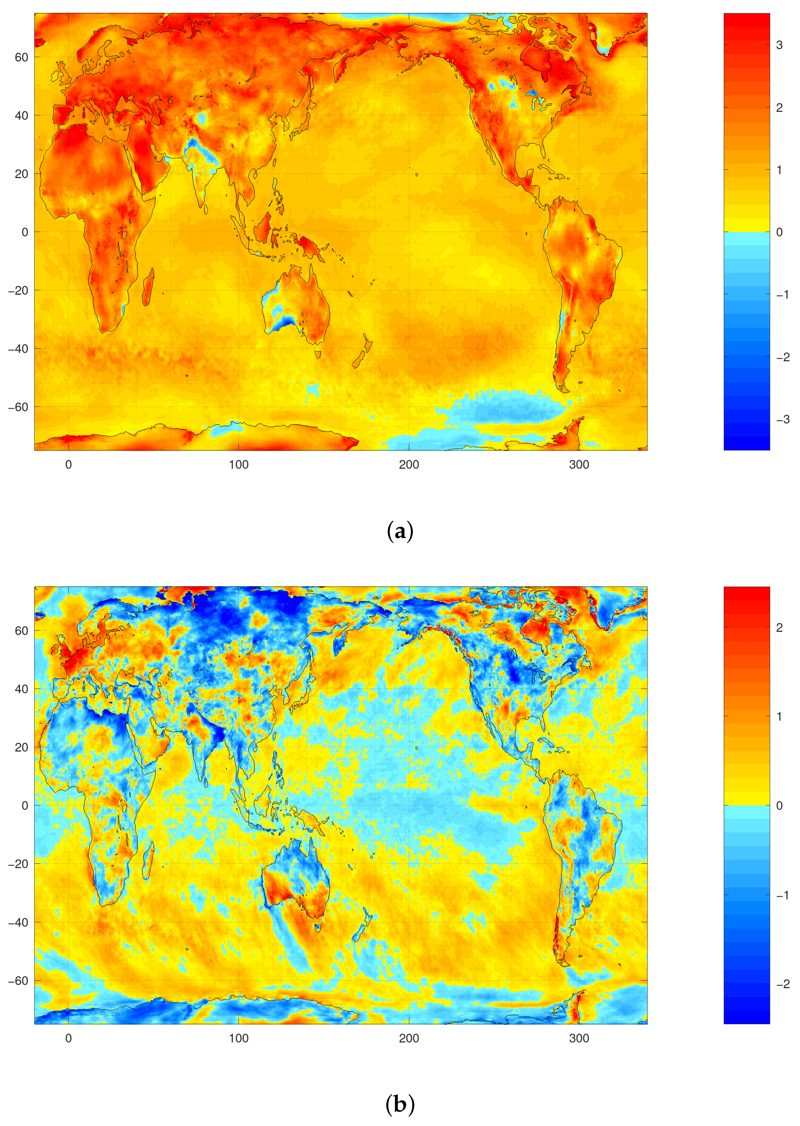
3.1. Mean Spatial Patterns

Typical summer daily maximum temperatures in ERA5, as summarized by T max 80 (Figure 1a), were, as expected, highest in subtropical and desert land areas and, at a given latitude, tended to be lower over the oceans as well as at high elevations. The difference Δ T between TXx and T max 80 had a distinctive behavior (Figure 1b). While higher over land than over the oceans (mean Δ T was 7.66 °C over land compared to only 2.26 °C over water), it was not necessarily higher in the deserts, but instead peaked at the poleward margins of continents, where summer conditions are dominated by flow from the nearby mild ocean but sometimes receive much hotter continental air. For example, western Europe, which experiences occasional heat waves associated with hot and dry Saharan air masses, tended to have higher summer temperature range Δ T than the Sahara itself, which is more consistently hot in summer.

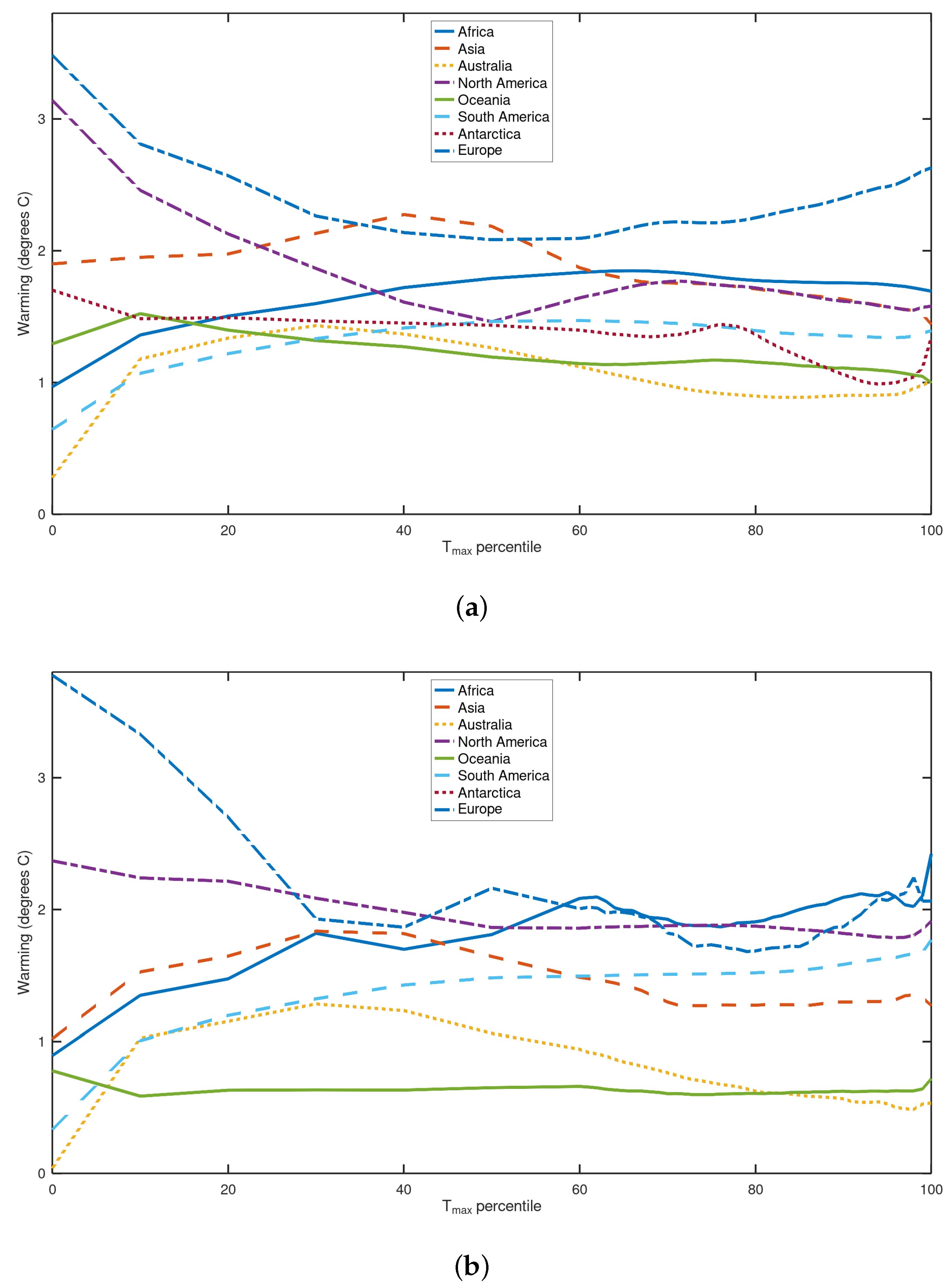
3.2. Warming and Amplification

The trend in T max 80 in ERA5 showed strong warming of 1–3 °C between 1959 and 2021 in most land regions, and warming of typically 0.5–1 °C over oceans (Figure 2a). High-latitude and desert regions tended to warm the most. Some land areas that showed little or no warming are those known to have experienced agricultural intensification and expansion of irrigated area, such as the northern Great Plains in North America and the Indus Valley [47,48], or enhanced sea breeze, such as coastal California [49,50]. ERA5 also showed less or no summer warming over the Laurentian Great Lakes, with cooling over Lake Superior, which is inconsistent with in situ and satellite data that show rapid summer warming there [51,52,53] and may point to problems in modeling or data assimilation over lakes in ERA5.
Meanwhile, the change A in Δ T between 1959 and 2021 in ERA5 showed pronounced local and regional differences, mostly in the range 2 to + 2 °C (Figure 2b). For example, A was positive over much of Europe, meaning that extreme warm temperatures increased faster than mean summer temperatures, but near zero over Italy and northern Scandinavia. A was negative over some irrigated areas, such as California’s Central Valley, the USA Midwest, and the Ganges Valley, but positive over others, such as the Indus valley and the Mississippi delta.
Overall, the warming in T max 80 between 1959 and 2021 in ERA5 averaged 1.62 °C over land and 0.71 °C over water. The amplification A averaged −0.23 °C over land and 0.10 °C over water, indicating that on average over land TXx increased more slowly than T max 80 while over ocean it increased more quickly. However, over both land and water, there are wide variations between positive and negative values (Figure 2b).
On continental scales, average A was significantly below zero over Asia and positive over Europe. When weighted by population, the average A was no longer significantly different from zero globally or over Asia and Europe, but was significantly above zero in Africa, Oceania, and South America (Table 1).
Grid cells that were at least partly equipped for irrigation (17% of the land area, but accounting for 89% of world population) had only slightly lower area-average amplification than other land grid cells (−0.12 versus −0.09 °C). Moreover, for the grid cells that were at least partly equipped for irrigation, there was little correlation between the fraction equipped for irrigation and amplification (the Spearman rank correlation between the two quantities was 0.008). Thus, globally, agricultural intensification as expressed in equipment for irrigation did not appear to be a major factor in explaining spatial variability in amplification.
To assess the sensitivity of the amplification quantities to the choice of T max percentiles considered compared to the 80th ( T max 80 ) and 100th (TXx) chosen here, the continental warming between 1959 and 2021 in ERA5 was also plotted across T max percentiles (Figure 3). For the most part, the warming rate is a relatively smooth function of the T max percentile. The largest differences between TXx and the 99th percentile are seen in Antarctica and in Africa with population weighting, both of which have TXx warming faster than the less extreme 99th percentile. For the most part, the amplification factor would be similar if the typical summer temperature was taken as the 70th or 90th as opposed to the 80th percentile, although in Europe with population weighting, this would make A less positive (Figure 3b). The lowest percentiles, corresponding to winter conditions in the extratropics, warmed much faster than the median in Europe and North America but similar to or less than the median in other continents, similar to what was found in earlier work based on station data [26].

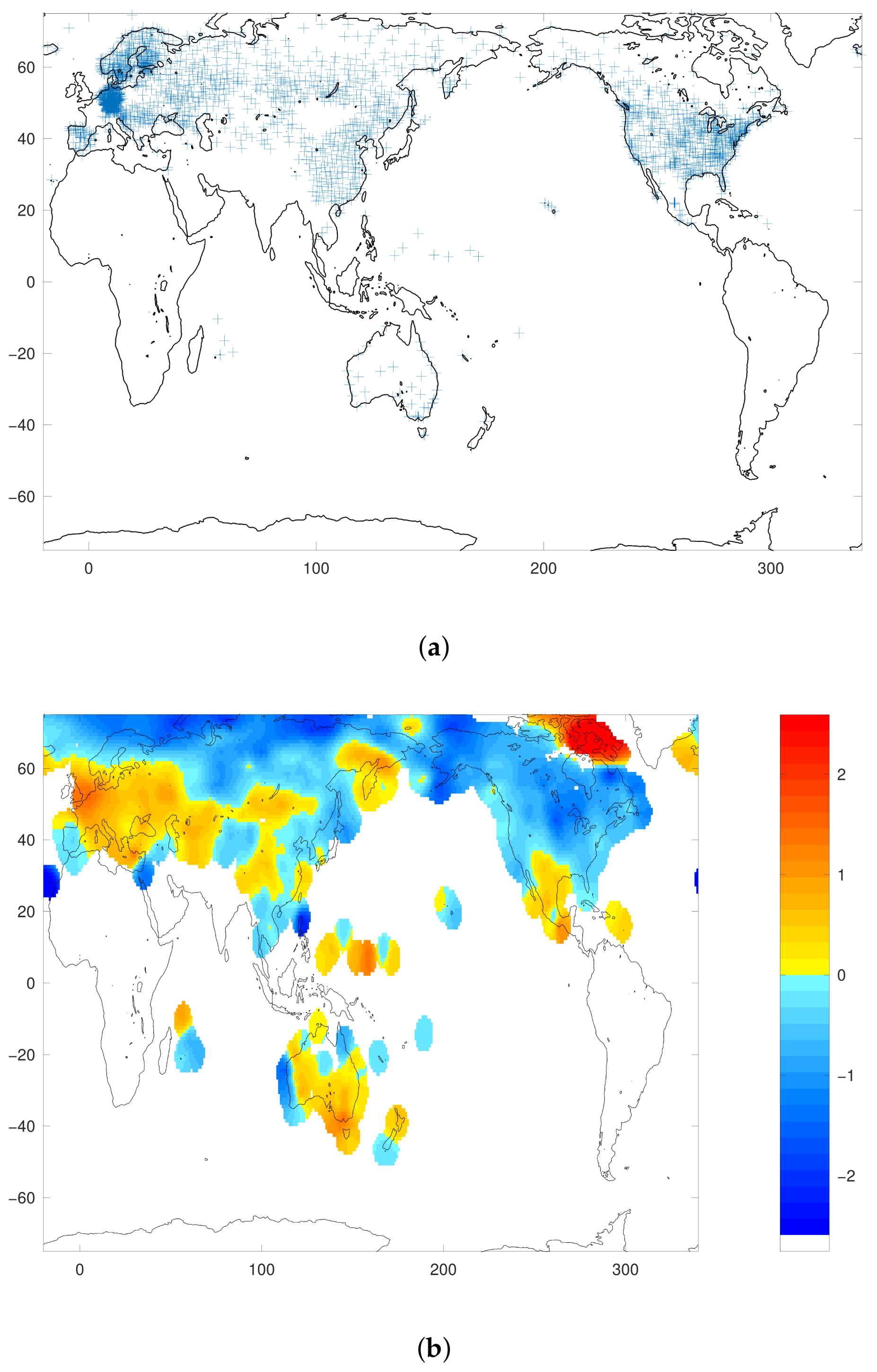
3.3. Comparison with GHCN-D Station Data

There were 2118 stations in GHCN-D with sufficiently complete daily maximum temperature data for 1959–2021. The stations were concentrated in the USA, Europe, and China, with some also in Siberia and Australia, but almost none in Africa and none in South America or the Indian subcontinent (Figure 4a). GHCN-D had somewhat larger mean Δ T than the corresponding ERA5 grid cells (9.95 vs. 9.44 °C), which is reasonable considering that a global reanalysis would miss some of the small-scale spatial and temporal variability that could drive up yearly extremes. ERA5 well captured the GHCN-D interstation variability in interannual-mean T max 80 (correlation of 0.971 between GHCN-D and subsampled ERA5) and Δ T (correlation of 0.890).
The average 1959–2021 warming in T max 80 for the GHCN-D stations compared well with ERA5 for the same grid cells (GHCN-D: 1.65 °C, ERA5: 1.67 °C), although the average amplification A at station locations was somewhat more positive in the reanalysis (GHCN-D: 0.03 °C, ERA5: 0.26 °C). The spatial distribution of A showed a strong positive correlation of 0.763 between GHCN-D stations and ERA5, and GHCN-D showed many of the same patterns as ERA5 of, for example, regions of negative A centered over northern Siberia and the northern Great Plains of the United States, and positive A over western Europe (Figure 4b).

4. Discussion

Based on ERA5, over land in 1959–2021, annual maximum temperatures TXx warmed about 3% more slowly than 80th percentile daily maxima T max 80 (by 1.56 versus 1.60 °C), for a negative mean amplification A ( 0.04 °C). This refines the current perception in the scientific literature that the hot extremes of the temperature distribution, such as TXx, are increasing at about the same rate as its center, and that temperature variability shows no obvious trend [23,54]. A possible physical reason for a slower increase in TXx over land is the nonlinearity with temperature of thermal radiation emission, such that at higher temperatures, a given radiative forcing is balanced by a smaller temperature increase. On the other hand, over water, TXx has warmed about 18% faster than T max 80 over the same period, for a positive mean A ( 0.13 °C). This could be due to the temperature range over water being characteristically much less than over land, so that the nonlinearity in thermal emission is less important, along with an increase in land-sea summer temperature contrast (as the land surface has warmed faster than the oceans) [55], such that the incursion of continental air can now lead to higher peak temperatures compared to the new overwater mean temperature. Weighting by population instead of land area, mean A was not significantly different from zero.
Along with the mean value for amplification A, there was pronounced regional variability. Some regions, including much of Europe, north-central India, the south-central United States, and inland southeast and southwest Australia, had annual maximum temperatures increasing much faster than typical summer temperatures (positive A). In other cases, such as over the Ganges basin, northeast Africa, the northern Great Plains of central North America, and much of Siberia, annual maxima have warmed much less (negative A). These regional differences can have important implications for the frequency of the most severe impacts on human and ecosystem health.
Ref. [56] found that hot days over tropical land warm more than the average day, which is attributed to a ’drier get hotter’ mechanism. This is based on the idea that the days with the highest temperature tend to be the driest ones (with low soil moisture), and therefore less of the additional heat can go to evaporating water, compared to average days in the moist tropics. This hypothesis is consistent with the positive mean populationweighted amplification seen over primarily tropical Africa, Oceania, and South America. However, plotting mean ERA5 amplification by latitude over land (not shown) did not reveal clear overall trends. Northwest Europe could be an example of an extratropical region that normally has abundant moisture during the hot season for evaporation that keep temperatures down, but can be subject to occasional drought that dominates TXx [57,58,59], explaining the strongly positive A there. Over water, by contrast, where the moisture supply does not limit evaporation, the trend was towards higher amplification in the mid-latitudes, which at least in the Northern Hemisphere possibly reflects the faster warming over land there that leads to relatively hotter available continental air. Climatemode experiments also show that the plant physiological response to rising CO2 levels, including higher water use efficiency, tends to increase TXx over Europe while decreasing it over central North America [60], which is broadly consistent with the trends shown here.
The strengths of this study include defining an amplification metric to exclude diurnal and seasonal effects, using a state-of-the-art reanalysis with high spatial and temporal resolution, and analysis at global and continental scales. On the other hand, many factors such as topography, biome, and soil type may also affect amplification, and could be examined in future research. Land cover and land use aspects such as urbanization [15] and irrigated agriculture [61,62], as well as atmospheric forcing agents such as aerosols [63], clearly affect amplification and also need to be considered. While the correlation of amplification with an area equipped for irrigation was investigated here and found to be small overall, it may be important regionally, depending for example on the seasonality of irrigation versus that of peak temperature.
In addition, by considering only temperature as an extreme heat metric, this study left out the role of humidity in aggravating heat stress. For example, while irrigation is modeled to mitigate hot temperature extremes, it also increases humidity and therefore potentially measures of humid heat extremes [34,37]. Moreover, amplification showed strong regional variability beyond the pattern associated with climate zones, likely due to local surface conditions and atmospheric circulation. For example, Europe, where heat extremes are associated with the flow of Saharan air from the south combined with local drought [58,64], showed particularly high amplification. Another hot spot of high A was in the southern Amazon basin, which could be associated with forest clearing and conversion to agriculture and pasture, which makes evapotranspiration far more seasonal [65,66,67].
The amplification measure considered here using ERA5 and station data could also be investigated in global climate model simulations. If climate models are able to accurately simulate observed regional variability in A, more confidence could be placed in their projections of future changes in A. It can be hypothesized that if global warming continues, the distribution of A will gradually shift over time as climate zones migrate [68,69] and moisture limitation of evaporation becomes more widespread in the tropics and temperate zones [70].
The comparison of temperature percentiles and their trends in ERA5 with station-based daily maximum temperature data showed substantial agreement between the reanalysis and station observation. Some discrepancies were identified, such as ERA5 having too little summer warming over the Great Lakes. These could be investigated further and hopefully corrected in future reanalysis versions.

5. Conclusions

It was found that over land, the maximum annual temperature tended to increase slightly more slowly than the 80th percentile maximum temperature, for a negative amplification (or dampening) of the hot temperature extremes. By contrast, over water, there was positive mean amplification. Specific continents and regions in the moist tropics and temperate mid-latitudes, such as much of Africa and Europe, showed positive amplification. Amplification could be affected by land-atmosphere feedbacks, including those associated with irrigated areas and with the physiological effects of rising CO2 concentrations on plant transpiration, as well as with regional circulation and land use changes, which need to be investigated in more detail. These findings provide a new target for climate model calibration, and insight for evaluating the changing risk of temperature extremes.

Funding

This research was funded by the National Oceanic and Atmospheric Administration Educational Partnership Program with Minority-Serving Institutions—Cooperative Science Center for Earth System Sciences and Remote Sensing Technologies under the Cooperative Agreement Grant numbers NA16SEC4810008 and NA22SEC4810016. The statements contained within this article are not the opinions of the funding agency or the United States government but reflect the author’s opinions.

Data Availability Statement

The data used in this research is available to download from its respective providers.

Conflicts of Interest

The author declares no conflict of interest. The funders had no role in the design of the study; in the collection, analyses, or interpretation of data; in the writing of the manuscript, or in the decision to publish the results.

References

  1. Tebaldi, C.; Hayhoe, K.; Arblaster, J.M.; Meehl, G.A. Going to the extremes. Clim. Chang. 2006, 79, 185–211. [Google Scholar] [CrossRef]
  2. Alexander, L.V.; Zhang, X.; Peterson, T.C.; Caesar, J.; Gleason, B.; Klein Tank, A.M.G.; Haylock, M.; Collins, D.; Trewin, B.; Rahimzadeh, F.; et al. Global observed changes in daily climate extremes of temperature and precipitation. J. Geophys. Res. 2006, 111, D05109. [Google Scholar] [CrossRef]
  3. McKinnon, K.A.; Rhines, A.; Tingley, M.P.; Huybers, P. The changing shape of Northern Hemisphere summer temperature distributions. J. Geophys. Res. Atmos. 2016, 121, 8849–8868. [Google Scholar] [CrossRef]
  4. Tamarin-Brodsky, T.; Hodges, K.; Hoskins, B.J.; Shepherd, T.G. Changes in Northern Hemisphere temperature variability shaped by regional warming patterns. Nat. Geosci. 2020, 13, 414–421. [Google Scholar] [CrossRef]
  5. Klein Tank, A.M.; Zwiers, F.W.; Zhang, X. Guidelines on Analysis of Extremes in a Changing Climate in Support of Informed Decisions for Adaptation; Technical Report; World Meteorological Organization: Geneva, Switzerland, 2009. [Google Scholar]
  6. Zhang, X.; Alexander, L.; Hegerl, G.C.; Jones, P.; Tank, A.K.; Peterson, T.C.; Trewin, B.; Zwiers, F.W. Indices for monitoring changes in extremes based on daily temperature and precipitation data. Wiley Interdiscip. Rev. Clim. Chang. 2011, 2, 851–870. [Google Scholar] [CrossRef]
  7. Seneviratne, S.I.; Zwiers, F.W. Attribution and prediction of extreme events: Editorial on the special issue. Weather Clim. Extrem. 2015, 9, 2–5. [Google Scholar] [CrossRef]
  8. Easterling, D.R. Global Data Sets for Analysis of Climate Extremes. In Extremes in a Changing Climate; AghaKouchak, A., Easterling, D., Hsu, K., Schubert, S., Sorooshian, S., Eds.; Springer: Dordrecht, The Netherlands, 2013; Volume 65, pp. 347–361. [Google Scholar] [CrossRef]
  9. Coumou, D.; Robinson, A. Historic and future increase in the global land area affected by monthly heat extremes. Environ. Res. Lett. 2013, 8, 034018. [Google Scholar] [CrossRef]
  10. Donat, M.G.; Alexander, L.V.; Yang, H.; Durre, I.; Vose, R.; Dunn, R.J.H.; Willett, K.M.; Aguilar, E.; Brunet, M.; Caesar, J.; et al. Updated analyses of temperature and precipitation extreme indices since the beginning of the twentieth century: The HadEX2 dataset. J. Geophys. Res. 2013, 118, 2098–2118. [Google Scholar] [CrossRef]
  11. Milagros de los Skansi, M.; Brunet, M.; Sigro, J.; Aguilar, E.; Groening, J.A.A.; Bentancur, O.J.; Geier, Y.R.C.; Amaya, R.L.C.; Jácome, H.; Ramos, A.M.; et al. Warming and wetting signals emerging from analysis of changes in climate extreme indices over South America. Glob. Planet. Chang. 2013, 100, 295–307. [Google Scholar] [CrossRef]
  12. Sillmann, J.; Kharin, V.V.; Zhang, X.; Zwiers, F.W.; Bronaugh, D. Climate extremes indices in the CMIP5 multi-model ensemble. Part 1: Model evaluation in the present climate. J. Geophys. Res. 2013, 118, 1716–1733. [Google Scholar] [CrossRef]
  13. Mistry, M. A High-Resolution Global Gridded Historical Dataset of Climate Extreme Indices. Data 2019, 4, 41. [Google Scholar] [CrossRef]
  14. Zaitchik, B.F.; Tuholske, C. Earth observations of extreme heat events: Leveraging current capabilities to enhance heat research and action. Environ. Res. Lett. 2021, 16, 111002. [Google Scholar] [CrossRef]
  15. Mishra, V.; Ganguly, A.R.; Nijssen, B.; Lettenmaier, D.P. Changes in observed climate extremes in global urban areas. Environ. Res. Lett. 2015, 10, 024005. [Google Scholar] [CrossRef]
  16. Habeeb, D.; Vargo, J.; Stone, B. Rising heat wave trends in large US cities. Nat. Hazards 2015, 76, 1651–1665. [Google Scholar] [CrossRef]
  17. Stillman, J.H. Heat Waves, the New Normal: Summertime Temperature Extremes Will Impact Animals, Ecosystems, and Human Communities. Physiology 2019, 34, 86–100. [Google Scholar] [CrossRef]
  18. Kennedy-Asser, A.T.; Andrews, O.; Mitchell, D.M.; Warren, R.F. Evaluating heat extremes in the UK Climate Projections (UKCP18). Environ. Res. Lett. 2020, 16, 014039. [Google Scholar] [CrossRef]
  19. Mueller, N.D.; Butler, E.E.; McKinnon, K.A.; Rhines, A.; Tingley, M.; Holbrook, N.M.; Huybers, P. Cooling of US Midwest summer temperature extremes from cropland intensification. Nat. Clim. Chang. 2015, 6, 317–322. [Google Scholar] [CrossRef]
  20. Thiery, W.; Visser, A.J.; Fischer, E.M.; Hauser, M.; Hirsch, A.L.; Lawrence, D.M.; Lejeune, Q.; Davin, E.L.; Seneviratne, S.I. Warming of hot extremes alleviated by expanding irrigation. Nat. Commun. 2020, 11, 290. [Google Scholar] [CrossRef]
  21. Wu, X.; Wang, L.; Yao, R.; Luo, M.; Li, X. Identifying the dominant driving factors of heat waves in the North China Plain. Atmos. Res. 2021, 252, 105458. [Google Scholar] [CrossRef]
  22. Oldenborgh, G.J.V.; Wehner, M.F.; Vautard, R.; Otto, F.E.L.; Seneviratne, S.I.; Stott, P.A.; Hegerl, G.C.; Philip, S.Y.; Kew, S.F. Attributing and Projecting Heatwaves Is Hard: We Can Do Better. Earth’s Future 2022, 10, e2021EF002271. [Google Scholar] [CrossRef]
  23. Seneviratne, S.I.; Zhang, X.; Adnan, M.; Badi, W.; Dereczynski, C.; Di Luca, A.; Ghosh, S.; Iskandar, I.; Kossin, J.; Lewis, S.; et al. Weather and climate extreme events in a changing climate. In Climate Change 2021: The Physical Science Basis. Contribution of Working Group I to the Sixth Assessment Report of the Intergovernmental Panel on Climate Change; Cambridge University Press: Cambridge, UK, 2021. [Google Scholar]
  24. Di Luca, A.; de Elía, R.; Bador, M.; Argüeso, D. Contribution of mean climate to hot temperature extremes for present and future climates. Weather Clim. Extrem. 2020, 28, 100255. [Google Scholar] [CrossRef]
  25. Di Luca, A.; Pitman, A.J.; de Elía, R. Decomposing Temperature Extremes Errors in CMIP5 and CMIP6 Models. Geophys. Res. Lett. 2020, 47, e2020GL088031. [Google Scholar] [CrossRef]
  26. Krakauer, N.Y. Shifting hardiness zones: Trends in annual minimum temperature. Climate 2018, 6, 15. [Google Scholar] [CrossRef]
  27. Dunn, R.J.H.; Willett, K.M.; Thorne, P.W.; Woolley, E.V.; Durre, I.; Dai, A.; Parker, D.E.; Vose, R.S. HadISD: A quality-controlled global synoptic report database for selected variables at long-term stations from 1973–2011. Clim. Past 2012, 8, 1649–1679. [Google Scholar] [CrossRef]
  28. Dunn, R.J.H.; Willett, K.M.; Parker, D.E.; Mitchell, L. Expanding HadISD: Quality-controlled, sub-daily station data from 1931. Geosci. Instrum. Methods Data Syst. 2016, 5, 473–491. [Google Scholar] [CrossRef]
  29. Hurvich, C.M.; Simonoff, J.S.; Tsai, C.L. Smoothing parameter selection in nonparametric regression using an improved Akaike information criterion. J. R. Stat. Soc. 1998, 60B, 271–293. [Google Scholar] [CrossRef]
  30. Krakauer, N.Y. Estimating climate trends: Application to United States plant hardiness zones. Adv. Meteorol. 2012, 2012, 404876. [Google Scholar] [CrossRef]
  31.  ERA5 Reanalysis (0.25 Degree Latitude-Longitude Grid). 2019. Available online: https://rda.ucar.edu/datasets/ds633.0/ (accessed on 3 January 2023). [CrossRef]
  32. Hersbach, H.; de Rosnay, P.; Bell, B.; Schepers, D.; Simmons, A.; Soci, C.; Abdalla, S.; Alonso-Balmaseda, M.; Balsamo, G.; Bechtold, P.; et al. Operational Global Reanalysis: Progress, Future Directions and Synergies with NWP; Technical Report 27; ECMWF: London, UK, 2018. [Google Scholar] [CrossRef]
  33. Domínguez-Castro, F.; Reig, F.; Vicente-Serrano, S.M.; Aguilar, E.; Peña-Angulo, D.; Noguera, I.; Revuelto, J.; van der Schrier, G.; El Kenawy, A.M. A multidecadal assessment of climate indices over Europe. Sci. Data 2020, 7, 125, Uses European Climate Assessment & Dataset (ECA&D) E-OBS gridded dataset and ERA5. [Google Scholar] [CrossRef] [PubMed]
  34. Mishra, V.; Ambika, A.K.; Asoka, A.; Aadhar, S.; Buzan, J.; Kumar, R.; Huber, M. Moist heat stress extremes in India enhanced by irrigation. Nat. Geosci. 2020, 13, 722–728. [Google Scholar] [CrossRef]
  35. Freychet, N.; Hegerl, G.; Mitchell, D.; Collins, M. Future changes in the frequency of temperature extremes may be underestimated in tropical and subtropical regions. Commun. Earth Environ. 2021, 2, 28. [Google Scholar] [CrossRef]
  36. Li, X.X. Heat wave trends in Southeast Asia during 1979–2018: The impact of humidity. Sci. Total Environ. 2020, 721, 137664. [Google Scholar] [CrossRef]
  37. Krakauer, N.Y.; Cook, B.I.; Puma, M.J. Effect of irrigation on humid heat extremes. Environ. Res. Lett. 2020, 15, 094010. [Google Scholar] [CrossRef]
  38. Menne, M.; Durre, I.; Vose, R.; Gleason, B.; Houston, T. An overview of the Global Historical Climatology Network-Daily database. J. Atmos. Ocean. Technol. 2012, 29, 897–910. [Google Scholar] [CrossRef]
  39. Jaffrés, J.B. GHCN-Daily: A treasure trove of climate data awaiting discovery. Comput. Geosci. 2019, 122, 35–44. [Google Scholar] [CrossRef]
  40. Durre, I.; Menne, M.J.; Gleason, B.E.; Houston, T.G.; Vose, R.S. Comprehensive automated quality assurance of daily surface observations. J. Appl. Meteorol. Climatol. 2010, 49, 1615–1633. [Google Scholar] [CrossRef]
  41. Doxsey-Whitfield, E.; MacManus, K.; Adamo, S.B.; Pistolesi, L.; Squires, J.; Borkovska, O.; Baptista, S.R. Taking Advantage of the Improved Availability of Census Data: A First Look at the Gridded Population of the World, Version 4. Pap. Appl. Geogr. 2015, 1, 226–234. [Google Scholar] [CrossRef]
  42. Center For International Earth Science Information Network-CIESIN-Columbia University. Gridded Population of the World, Version 4 (GPWv4): Population Count, Revision 11; Columbia University: New York, NY, USA, 2018. [Google Scholar] [CrossRef]
  43. Siebert, S.; Döll, P.; Hoogeveen, J.; Faures, J.M.; Frenken, K.; Feick, S. Development and validation of the global map of irrigation areas. Hydrol. Earth Syst. Sci. 2005, 9, 535–547. [Google Scholar] [CrossRef]
  44. Siebert, S.; Burke, J.; Faures, J.M.; Frenken, K.; Hoogeveen, J.; Döll, P.; Portmann, F.T. Groundwater use for irrigation—A global inventory. Hydrol. Earth Syst. Sci. 2010, 14, 1863–1880. [Google Scholar] [CrossRef]
  45. Wilcox, R. A Note on the Theil-Sen Regression Estimator When the Regressor Is Random and the Error Term Is Heteroscedastic. Biom. J. 1998, 40, 261–268. [Google Scholar] [CrossRef]
  46. Sen, P.K. Estimates of the regression coefficient based on Kendall’s tau. J. Am. Stat. Assoc. 1968, 63, 1379–1389. [Google Scholar] [CrossRef]
  47. Chen, L.; Dirmeyer, P.A. Global observed and modelled impacts of irrigation on surface temperature. Int. J. Climatol. 2019, 39, 2587–2600. [Google Scholar] [CrossRef]
  48. Albaladejo-García, J.A.; Alcon, F.; Martínez-Paz, J.M. The Irrigation Cooling Effect as a Climate Regulation Service of Agroecosystems. Water 2020, 12, 1553. [Google Scholar] [CrossRef]
  49. Lebassi-Habtezion, B.; González, J.; Bornstein, R. Modeled large-scale warming impacts on summer California coastal-cooling trends. J. Geophys. Res. 2011, 116, D20114. [Google Scholar] [CrossRef]
  50. Potter, C. Understanding climate change on the California coast: Accounting for extreme daily events among long-term trends. Climate 2014, 2, 18–27. [Google Scholar] [CrossRef]
  51. Mason, L.A.; Riseng, C.M.; Gronewold, A.D.; Rutherford, E.S.; Wang, J.; Clites, A.; Smith, S.D.P.; McIntyre, P.B. Fine-scale spatial variation in ice cover and surface temperature trends across the surface of the Laurentian Great Lakes. Clim. Chang. 2016, 138, 71–83. [Google Scholar] [CrossRef]
  52. Zhong, Y.; Notaro, M.; Vavrus, S.J. Spatially variable warming of the Laurentian Great Lakes: An interaction of bathymetry and climate. Clim. Dyn. 2018, 52, 5833–5848. [Google Scholar] [CrossRef]
  53. White, C.; Heidinger, A.; Ackerman, S.; McIntyre, P. A Long-Term Fine-Resolution Record of AVHRR Surface Temperatures for the Laurentian Great Lakes. Remote Sens. 2018, 10, 1210. [Google Scholar] [CrossRef]
  54. Alexander, L.; Perkins, S. Debate heating up over changes in climate variability. Environ. Res. Lett. 2013, 8, 041001. [Google Scholar] [CrossRef]
  55. Byrne, M.P.; O’Gorman, P.A. Trends in continental temperature and humidity directly linked to ocean warming. Proc. Natl. Acad. Sci. USA 2018, 115, 4863–4868. [Google Scholar] [CrossRef]
  56. Byrne, M.P. Amplified warming of extreme temperatures over tropical land. Nature Geosci. 2021, 14, 837–841. [Google Scholar] [CrossRef]
  57. Fischer, E.M.; Seneviratne, S.I.; Vidale, P.L.; Luthi, D.; Schar, C. Soil moisture—Atmosphere interactions during the 2003 European summer heat wave. J. Clim. 2007, 20, 5081–5099. [Google Scholar] [CrossRef]
  58. Zampieri, M.; D’Andrea, F.; Vautard, R.; Ciais, P.; de Noblet-Ducoudré, N.; Yiou, P. Hot European summers and the role of soil moisture in the propagation of Mediterranean drought. J. Clim. 2009, 22, 4747–4758. [Google Scholar] [CrossRef]
  59. Stéfanon, M.; Drobinski, P.; D’Andrea, F.; Lebeaupin-Brossier, C.; Bastin, S. Soil moisture-temperature feedbacks at meso-scale during summer heat waves over Western Europe. Clim. Dyn. 2014, 42, 1309–1324. [Google Scholar] [CrossRef]
  60. Lemordant, L.; Gentine, P. Vegetation Response to Rising CO2 Impacts Extreme Temperatures. Geophys. Res. Lett. 2018, 46, 1383–1392. Available online: https://agupubs.onlinelibrary.wiley.com/doi/pdf/10.1029/2018GL080238 (accessed on 3 January 2023). [CrossRef]
  61. Lobell, D.B.; Bonfils, C.J.; Kueppers, L.M.; Snyder, M.A. Irrigation cooling effect on temperature and heat index extremes. Geophys. Res. Lett. 2008, 35. [Google Scholar] [CrossRef]
  62. Thiery, W.; Davin, E.L.; Lawrence, D.M.; Hirsch, A.L.; Hauser, M.; Seneviratne, S.I. Present-day irrigation mitigates heat extremes. J. Geophys. Res. Atmos. 2017, 122, 1403–1422. [Google Scholar] [CrossRef]
  63. Xu, Y.; Lamarque, J.F.; Sanderson, B.M. The importance of aerosol scenarios in projections of future heat extremes. Clim. Chang. 2018, 146, 393–406. [Google Scholar] [CrossRef]
  64. Hirschi, M.; Seneviratne, S.I.; Alexandrov, V.; Boberg, F.; Boroneant, C.; Christensen, O.B.; Formayer, H.; Orlowsky, B.; Stepanek, P. Observational evidence for soil-moisture impact on hot extremes in southeastern Europe. Nat. Geosci. 2011, 4, 17–21. [Google Scholar] [CrossRef]
  65. Fan, Y.; Miguez-Macho, G. Potential groundwater contribution to Amazon evapotranspiration. Hydrol. Earth Syst. Sci. 2010, 14, 2039–2056. [Google Scholar] [CrossRef]
  66. Markewitz, D.; Devine, S.; Davidson, E.A.; Brando, P.; Nepstad, D.C. Soil moisture depletion under simulated drought in the Amazon: Impacts on deep root uptake. New Phytol. 2010, 187, 592–607. [Google Scholar] [CrossRef]
  67. Swann, A.L.S.; Koven, C.D. A Direct Estimate of the Seasonal Cycle of Evapotranspiration over the Amazon Basin. J. Hydrometeorol. 2017, 18, 2173–2185. [Google Scholar] [CrossRef]
  68. Beck, H.E.; Zimmermann, N.E.; McVicar, T.R.; Vergopolan, N.; Berg, A.; Wood, E.F. Present and future Köppen-Geiger climate classification maps at 1-km resolution. Sci. Data 2018, 5, 180214. [Google Scholar] [CrossRef] [PubMed]
  69. Cui, D.; Liang, S.; Wang, D. Observed and projected changes in global climate zones based on Köppen climate classification. WIREs Clim. Chang. 2021, 12, e701. [Google Scholar] [CrossRef]
  70. Dai, A. Increasing drought under global warming in observations and models. Nat. Clim. Chang. 2013, 3, 52–58. [Google Scholar] [CrossRef]
Figure 1. (a) ERA5 mean T max 80 (°C), 1959–2021. (b) ERA5 mean difference between TXx and T max 80 (°C), 1959–2021.
Climate 11 00042 g001
Figure 2. (a) Smoothed ERA5 change in T max 80 (K), 1959–2021. (b) Smoothed ERA5 change in the difference between TXx and T max 80 (K), 1959–2021.
Climate 11 00042 g002
Figure 3. (a) Smoothed ERA5 change in different percentiles of T max , 1959–2021, by continent (area-weighted average), showing every 10th percentile up to the 60th, then every percentile. The 0th percentile corresponds to the coldest T max of each year and the 100th percentile to the annual maximum temperature TXx. (b) Same, but using population-weighted averages.
Climate 11 00042 g003
Figure 4. (a) Locations of GHCN-D stations available to compare with ERA5. (b) Change in the difference between TXx and T max 80 (°C), 1959–2021, based on spatial interpolation of GHCN-D stations. In the interpolation scheme, station values were weighted based on distance to each interpolation point with an exponential decay length scale of 2°. Interpolation was not performed for grid points over 4° away from a GHCN-D station.
Climate 11 00042 g004
Table 1. Smoothed change in T max 80 , TXx, and in their difference (amplification A) over 1959–2021 in ERA5 by water/land and continent.
Δ T max 80 Δ TXxA
Water0.720.850.13 *
Land1.60 (0.82)1.56 (0.92)−0.04 * (0.10)
Africa1.71 (1.90)1.69 (2.40)−0.02 (0.49 *)
Asia1.68 (1.15)1.46 (1.27)−0.22 * (0.12)
Australia0.01 (0.39)1.00 (0.52)0.99 (0.13)
North America1.70 (1.43)1.57 (1.92)−0.13 (0.59)
Oceania1.32 (0.61)1.13 (0.72)−0.19 (0.11 *)
South America1.10 (1.20)1.04 (1.44)−0.06 (0.25 *)
Antarctica1.341.30−0.05
Europe2.19 (1.70)2.48 (2.14)0.29 * (0.44)
The values in parentheses are population-weighted averages; the other values are area-weighted averages. Starred values of A are significantly different from zero at the 0.05 level (two-tailed).
Disclaimer/Publisher’s Note: The statements, opinions and data contained in all publications are solely those of the individual author(s) and contributor(s) and not of MDPI and/or the editor(s). MDPI and/or the editor(s) disclaim responsibility for any injury to people or property resulting from any ideas, methods, instructions or products referred to in the content.

