Abstract
Central Oklahoma is undergoing investment in new intermodal transportation and rehabilitation of its infrastructure. Despite a highly variable historical climate, future changes resulting from anthropogenic climate change may be outside of the range for which infrastructure was designed. We examined 21st century trends, focusing on weather and climate extremes of demonstrated importance to transportation professionals as identified through expert input. We assessed trends from a suite of 15 global climate models (GCMs) using two emissions scenarios and two high-resolution statistically downscaled datasets. This ensemble provided a quantitative range for potential future climate conditions whilst revealing uncertainties associated with different models and downscaling methods. Our results support the general consensus of a reduction in the frequency of cold temperatures, freeze–thaw cycles, and winter weather; however, for the latter, there is not necessarily a reduction in intensity. Extreme heat days (e.g., days ≥100 °F) increased by factors of 3–6, with this upper range associated with high greenhouse gas emissions, while the seasonal duration of extreme heat extended by 4–10 weeks. Projected return intervals for heavy rainfall increased in frequency and magnitude in the mid and late 21st century. Although the contribution of the emissions pathway to these changes is evident, different extreme value distributions and the varying simulations of precipitation from the GCMs have a large effect on magnitudes, leading to a range of possible futures to consider in infrastructure design. Precipitation metrics, particularly at the extremes, were more sensitive to the selection of downscaled data, as compared with temperature metrics. Our approach represents a resource for transportation professionals seeking to identify changing risk probabilities at regional to local scales, as a precursor to planning and adaptation.
1. Introduction
The transportation sector employs weather and climate information in the planning, design, and maintenance of resources and assets. Extreme weather is associated with the degradation or destruction of infrastructure and in delays, diversions, or accidents during transit [1,2,3]. Recent extreme events, such as excessive heat, severe winter weather, coastal storm surge, and extreme precipitation, have been implicated in increasing costs to state Departments of Transportation (DOTs) [4]. Shifts in the frequency and intensity of extreme events are anticipated in association with anthropogenic climate change [5,6], and it is increasingly recognized that historical climatological records do not contain good analogues for future conditions [7,8]. This shift from historically relied-upon “stationarity” may result in poor performance and reduced lifetimes for infrastructure designed using historical data.
In response to these stressors, there is a growing body of literature and resources that contextualize climate change impacts at the regional scale for decision support. A variety of approaches have been implemented, from the use of climate assessments to direct analyses of statistically downscaled climate projections derived from global climate models (GCMs). For example, vulnerabilities of transportation assets to climate stressors have been assessed using indicators and thresholds [7,8,9,10,11,12], and case studies have demonstrated how infrastructure, safety, or maintenance are sensitive to specific stressors. Despite the increasing abundance of resources and knowledge nationally, there are comparatively few transportation and infrastructure analyses that have directly incorporated climate data across the South Central United States [13,14].
Here, we developed a series of tailored climate projections for central Oklahoma, including the Oklahoma City (OKC) metropolitan area. Our research did not apply to a specific management challenge; rather, it provides a quantitative regional-to-local-scale climate change resource. We posit the following questions: (a) What adverse meteorological conditions and thresholds are of particular relevance and importance to transportation in this region; and (b) What are the trends and range of projections associated with these events of high concern? Due to their particular propensity for disruption, the variables and thresholds we examined focused on extremes, their selection guided by a survey disseminated to transportation professionals. We evaluated the range of plausible climate futures and uncertainties for particular variables through use of multiple GCMs, two emissions scenarios, and two publicly available statistical downscaling (hereafter, SD) techniques.
Our region was selected based on its ongoing investments in infrastructure replacement and rehabilitation. Based on the American Society for Civil Engineers (ASCE) ‘scorecard’ [15], OKC was previously ranked high in the number of deficient bridges for a city of 1–2 million people, and on average, urban roads were rated as ‘fair’ for pavement condition. Despite limitations posed by budget constraints, current and planned infrastructure projects are hardening, restoring, and replacing key assets (e.g., OK House Bills HB2248 and 2249, 2012), to the extent that the most recent ASCE report [16] notes clear improvement in bridge and road infrastructure. The state’s long-term transportation plan [17] identified infrastructure investment needs between 2015 and 2040, including the replacement of over 1800 bridges and 6400 miles of roadway, in addition to resurfacing and the introduction of light rail transit in downtown Oklahoma City. Many of these investments are, and will, improve infrastructure throughout the state, but their expected lifetimes of multiple decades places them under the influence of a changing climate. The proactive incorporation of climate-related risk is increasingly being recognized by federal and state agencies for the improved adaptation and mitigation of premature and expensive damage [16,18,19]. Quantitative regional-scale information is needed to assess these risks.
Our assessment identified the potential magnitude, scale, and range of climate impacts for transportation planners in central Oklahoma using techniques and data applicable to other regions. We recognize that the practical application of this information requires buy-in from multiple agents, and its implementation in infrastructure projects is not necessarily straightforward, partially due to inherent uncertainties in climate projections and the use of non-standard data. Other studies have highlighted challenges and suggested strategies for incorporating climate projections [18,19,20,21,22]. Section 2 summarizes expert input to the project, including our selection of thresholds and variables, and describes climate data acquisition and analysis. Section 3 details regional climate projections, and Section 4 discusses results within the context of transportation impacts. We conclude with a summary of the major findings in Section 5. The Supplementary Materials are available online.
2. Materials and Methods
2.1. Weather and Climate Information Needs Survey
Transportation-relevant weather and climate information was solicited from experts through an online survey entitled “Weather and Climate Data Needs for Transportation,” developed using Qualtrics (https://www.qualtrics.com, first accessed on 1 June 2015) [23], Section 2.1. We refined the survey through testing and feedback from colleagues at the South Central Climate Adaptation Science Center, Southern Climate Impacts Planning Program, and Southern Plains Transportation Center. The latter center released the online survey from September to December 2015 throughout U.S. DOT Region 6 via their email list server. In total, 57 respondents started the survey, with 62% completing the survey in full (38% in part). The relatively small sample size likely results from no prior relationship between the authors and many agencies solicited. However, those who participated provided substantive feedback.
The survey first collected basic demographic information. Then, participants ranked the most hazardous weather conditions from their professional perspective and assigned thresholds, if known, to hazardous temperature and precipitation conditions. Two questions asked respondents to rank, in order of perceived importance, various transportation-relevant weather and climate variables that have significant adverse impacts. Then, participants ranked the variables and indices they most desired from climate information. Further queries prompted participants to evaluate their current climate data resources, potential future needs, and opinions on data usability and reliability (Appendix A, Figure A1, Figure A2 and Figure A3). Respondents included transportation and engineering researchers (46%), construction engineers (30%), maintenance (26%), and infrastructure experts (22%); as well as other employees (22% self-identifying as in planning, operations, and urban design). The majority of completed surveys had respondents from Oklahoma (80%) and Texas (6%). There were 1–2 responses each from Arkansas, Louisiana, and New Mexico.
Total responses changed by variable, with a mean of n = 34 (60% of respondents), suggesting that some respondents skipped a variable that was not applicable or with unknown impact. The top 10 variables of concern, from highest to lowest, were: (1) heavy rainfall/flooding; (2) snowstorms; (3) extreme heat/maximum surface temperature; (4) freeze–thaw cycles; (5) freezing rain; (6) wind speed/high wind; (7) cold extremes/minimum surface temperature; (8) thunderstorms; (9) tornado; and (10) heating degree days, shown in Appendix A, Figure A1. With most respondents from Oklahoma, this ranking reflected extremes common to the state. Heavy precipitation was particularly salient due to repeated rounds of excessive rainfall and flooding during 2015 [24]. The survey also identified that winter events, although comparatively rare in the southern United States, were consistently among the top concerns.
After establishing key variables, participants used their experience to identify a typical threshold to distinguish hazardous conditions from normal operations for hot and cold temperatures (in °F) and for rainfall, snow, and ice (in inches or return periods). Many respondents left this question blank (n~20–24) if they did not know or have an applicable threshold. The most-cited threshold was 100 °F (37.8 °C) for hot temperatures and 32 °F (0 °C) for cold temperatures (Figure S2). For precipitation, respondents volunteered a wider range of values (not shown), as expected across a region with a large gradient in precipitation from southeast to northwest. For freezing rain, results suggested that even a glaze (between 0.01 and 0.25 inches, or 0.25 to 6.3 mm) is detrimental, with ≥0.25 inches (6.3 mm)—the current National Weather Service (NWS) criterion for an ice storm—ranking second. Snowfall thresholds of ≤5 inches (126 mm, per 24 h period) were noted by nearly 75% of respondents, with a few supplying much higher amounts, e.g., ≥10 inches (252 mm). For rainfall thresholds, 42% used an hourly rainfall rate, typically ≥1 inch (25.2 mm) per hour. Thirty percent used daily rainfall or event total, typically 3–8 inches over 24 h or a single event. Other respondents gave return-period thresholds of 1-in-50-year and 1-in-100-year events. Our results suggested that precipitation thresholds were highly contextualized to sub-discipline, location, or application (e.g., highway safety versus culvert design), consistent with views of non-transportation decision-makers [25]. Subsequently, multiple precipitation products would be most useful for a range of users.
Although the small sample size precluded statistical assessment, the expert guidance informed our choice of variables and the types of data products to generate. For this study, we selected those top-10 variables from the survey that could be derived from daily temperature and precipitation—standard variables available in gridded observations and SD climate projections. Thus, we evaluated heavy precipitation, winter precipitation (ice/snow), cold and hot extremes, and freeze–thaw cycles.
2.2. Climate Data
We used both historical observations (of at least 30 years duration) and future climate projections, as detailed in Supplementary Table S1. Climate model data are publicly available statistically downscaled global climate model (GCM) projections. Statistical downscaling approaches vary in statistical techniques and complexity [26]; we chose two ‘Constructed Analogue’ (CA) datasets that are widely used by decision makers: Multivariate Adaptive Constructed Analogues (MACA) [27] and Localized Constructed Analogues (LOCA) [28]. Both techniques identify local, high-resolution analogues associated with the coarse-resolution GCM atmospheric patterns, but with variations in the exact methodology.
MACA uses multivariate statistics to construct analogues, preserving the time sequences of events and atmospheric patterns simulated by the GCM, while correcting biases associated with terrain and resolution, thus better capturing the observed magnitudes of temperature and precipitation. MACA applies 20 GCMs from the Coupled Model Inter-comparison Project Phase 5 (CMIP5) [29], with 6.6 km horizontal grid spacing and daily temporal resolution, using Livneh (2013) [30] observations as the training data (i.e., MACAv2LIVNEH). Five of the twenty models were excluded based on their poor simulation of past climate in the South Central United States, as per Mullens and McPherson (2019) [31]. We analyzed data downscaled from the 15 remaining models for two representative concentration pathways (RCPs) [32], or future scenarios. RCP4.5 is a ‘mid-range’ future whereby some greenhouse gas emissions abatement is anticipated, and RCP8.5 is a ‘high’ emissions pathway representing a fossil-fuel-intensive world.
The secondary SD dataset was the Localized Constructed Analogues (LOCA) technique, developed by Pierce et al. [28,33]. LOCA’s downscaling approach also involves multivariate statistics, identifying regional analogues from gridded observations. LOCA differs from MACA in that it directly downscales the model-projected climatology change fields. Additionally, it applies a smaller spatial radius for its analog days and model fields.
Thus, our sampling accounted for a range of future emissions scenarios (RCP 4.5 and 8.5), model variability (15 distinct GCMs), and SD techniques (MACA and LOCA), all of which contribute to the expected range in the variability of magnitude, timing, and spatial extent of future climate-related impacts. Finally, to highlight some subsets of plausible futures (in addition to multi-model averages and ranges), we used the scenario approach of Mullens and McPherson [31] for the study area, grouping models into specific categories (‘Hot/Dry’ (HD) and ‘Warm/Wet’ (WW)) that represent a spread of plausible futures. The Supplementary Materials (Figures S1–S3, Table S2, available online) detail our subsetting approach.
2.3. Domain and Temporal Range
For most variables, we evaluated three 30-year reference periods: a ‘historical’ period from 1971 to 2000, a ‘mid-century’ period from 2021 to 2050, and a ‘late-century’ period from 2061 to 2090. Where timeseries were used, we included the full period 1960–2099. For the reference periods, more recent climate products use a historical climatology from 1981 to 2010; however, we chose a period that did not conflate the simulation periods in CMIP5, which ended their historical simulation in 2005. The mid-century period overlaps part of Oklahoma DOT’s 8-year strategic construction plan [34], and its 2015–2040 long-term transportation plan [17], spanning the expected lifespan of assets such as roadways and bridge pavements, railroad tracks, and some equipment. High-value durable infrastructure, such as culverts, bridges, and buildings, have lifetimes extending into the late-century period.
We aggregated the gridded data (i.e., gridded observations and downscaled datasets) into the 13-county Oklahoma Climate Division 5 (CD5 Figure 1) to present representative results to transportation stakeholders. Climate divisions (CDs) are easily recognizable by many decision-makers and reflect regions of similar climate and geography [31,35]. Although the CD-average does not reflect variables at a specific location, our interest was mesoscale temperature and average precipitation trends over time rather than micro- or urban-scale effects. Extreme precipitation is also better estimated through sampling from more grid boxes across each CD (see Section 3) Finally, extreme precipitation return periods are based on extrapolation of both maximum annual values and the top 5% values annually over the CD.
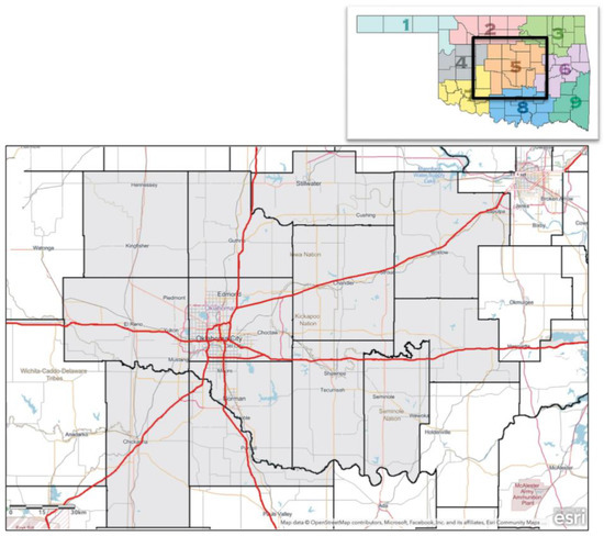
Figure 1.
Main panel: Domain (light grey shading), covering Oklahoma Climate Division 5 and overlain with counties, select cities, and roads. White areas are outside the bounds of the domain. Map and base layers are courtesy of ArcGIS online. Subsidiary panel shows the location of the domain within Oklahoma State (image courtesy of the Oklahoma Climatological Survey).
3. Results
3.1. Temperature and Freeze–Thaw Cycles
3.1.1. Freeze–Thaw Cycles
Based on a 1971–2000 average, central Oklahoma experiences approximately 65–70 freeze–thaw cycles (FTCs) per year, defined as a day with Tmin < 32 °F (0 °C) and Tmax > 32 °F, as in Hershfield (1974) [36]. Air temperatures are typically measured or simulated 2 m above ground; therefore, the data precluded us from obtaining a ‘true’ surface measurement. FTCs are associated with the degradation of road and bridge surfaces, particularly in the presence of moisture. FTC frequency increases from the southeast to northwest across OK CD5 [23]. In the past 70 years, annual FTCs have ranged from 45 to 90 days (Supplementary Figure S4). ‘Enhanced freeze–thaw cycles’ (EFTCs), defined by Haley (2011) [37] as daily Tmin < 23 °F (−5 °C) and Tmax > 41 °F (5 °C), range from 4 to 25 days, or about one in every five FTCs. Since the late 1940s, there has been a decrease in FTC and EFTC days, particularly the former, averaging a decline of 1 day per decade, a trend that stabilized after the 1980s (see online Supplementary Materials).
Figure 2 shows future projections of monthly FTCs over October–March for RCP4.5 (Figure 2a) and RCP8.5 (Figure 2b), with annual multi-model mean totals below each bar plot. Monthly and annual averages of FTCs and EFTCs decrease throughout the 21st century; however, natural variability continues to affect interannual magnitudes. By mid-century, the multi-model and multi-SD annual averages will decrease by approximately 20% (model range 7–28%), and are similar in magnitude regardless of the emissions pathway. In contrast, the magnitude of late 21st century changes strongly depends on the emissions pathway. FTCs in the RCP4.5 scenario decrease from 9% and 40% annually with a mean of 28%, while RCP8.5 shows a multi-model mean decrease of nearly 50% annually, with a range of 23–60%. Monthly projections depicted in Figure 2 suggest that the largest FTC decreases occur in early winter and early spring (e.g., November–December, March–April), with the smallest change during peak winter months when temperatures remain cool enough to permit night-time freezing. Incorporating the climate subsets indicates no systematic distinction between the hot-dry (HD) and warm-wet (WW) subsets of the models, except during November–February, when the HD models produce fewer FTC days, resulting from a greater magnitude of warming in that subset. WW models are more mixed, showing no particular tendency. We speculate that while the more moderate degree of warming in those models may favor less reduction in FTC events, a wetter future climate is potentially cloudier, thus reducing the number of night freezes. These compensating mechanisms will act differently, depending on the seasonal timing of cold weather, and their representation in GCMs.
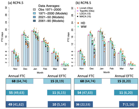
Figure 2.
Bar plot (top) displays the historical observed (asterisk for Livneh, box and triangle for TopoWx, and gray bar for model ensemble average; 1971–2000) and projected monthly (November–April) total freeze–thaw cycles for (a) RCP4.5 and (b) RCP8.5. Mean values from each MACA (dots) and LOCA (squares) projection are shown, with different shading for HD and WW models. Bottom schematics represent the annual multi-model means for (a,b) above, with FTC (left) and EFTC (right) for the three reference periods and their respective scenarios with the total sample spread (low, high) in parenthesis.
3.1.2. Annual Highest and Lowest Temperatures
Figure 3 displays a time series (1960–2099) of the highest daily high temperature and the lowest daily low temperature in each year (a measure of peak annual temperature range). The spread of these values in the SD projections corresponds to the interannual variability of the observations, implying that models represent the magnitude range well. Livneh and MACA both have median historical annual ranges of 55.8 °C, while LOCA’s range is larger at 57.3 °C. The June–August and December–February means increase by 5–10 °C by 2100. LOCA projections show a cold bias in peak minimum temperatures throughout the time series, particularly during the historical period, which helps to explain its larger annual range, whereas MACA projections produce higher maximum temperatures, especially mid to late 21st century. Minimum temperatures below −17 °C (0 °F) at the end of the century are still simulated in RCP4.5 (Figure 3a) but are exceptionally rare in RCP8.5 (Figure 3b). The annual maximum air temperature averages are near 40 °C (105 °F) in central Oklahoma for 1971–2000, 43–44 °C by the mid-21st century, but with a spread of projections which implies the increased frequency of very high temperatures (>43.3 °C, 110 °F). By late century, with RCP8.5, the peak annual maximum rises to 47 °C (~115 °F), with some potential for temperatures over 50 °C. The magnitude of annual temperature variation reflects the historical period for both SD methods, with little difference in their distributions. For example, the mid- and late 21st century median ranges under the RCP8.5 pathway for MACA were 57 °C and 56.8 °C, respectively, and for LOCA 57.2 °C and 57.6 °C, while measures of distribution such as skewness and kurtosis yielded generally similar results, with evidence of a slight positive skew, and a kurtosis that increased for both SD methods during the mid-21st century but retracted back to near-historical levels in the late 21st century (this was true of both emissions pathways). This indicates that the entire distribution by the late 21st century is simply shifted to higher maximum and minimum temperatures without notable sustained changes in its shape. Finally, the smoothed average (using Friedman’s super-smoothing R function [38]) of each time series of WW and HD subsets of projections indicates that HD (WW) models generally show a faster (slower) rise in hot and cold temperatures over time. Using an example of maximum temperatures under RCP8.5, HD is recorded as +7.8 °C/140 years versus +6.3 °C/140 years for WW (based on differences in the mean of the first and last decades of the record), compared with 7.6 °C/140 years for the total multi-model average. While cool temperatures under both emissions pathways scale similarly to the above, with HD subsets showing the greatest warming trend, this is not the case for the RCP4.5 high temperature results, which yield little differences in these subsets and the multi-model average.
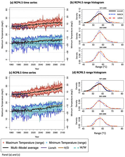
Figure 3.
Time series (left) of historical and future climate model projections (1960–2099) in highest daily maximum, (June–August) and lowest daily minimum temperatures (December–February) in °C. Panel (a) is RCP4.5; panel (c) is RCP8.5. Lines depict the multi-model mean (black line) and the shaded polygons indicated the maximum–minimum temperature range across the full ensemble of projections, for MACA projections only (shaded + stippling), and for LOCA projections only (shaded). Time series for HD and WW model average values are smoothed using the ‘supsmu’ function in R. Observations (Livneh) is the thick purple line. On the right are probability density distributions of annual temperature ranges during 1971–2000 (top), 2021–2050 (middle) and 2061–2090 (bottom) for (b) RCP4.5 and (d) RCP8.5. Livneh, MACA and LOCA line legend is shown in the top panel of (b).
3.1.3. Extreme Heat
The Oklahoma City metropolitan area experiences an average of 10 days per year with temperatures ≥37.8 °C (100 °F) (Oklahoma Mesonet [39], 1981–2010), defined here as ‘extreme heat days.’ Historically, the hottest in situ air temperature in the city was 45°C (113 °F), recorded in both 1936 and 2012 [40]. Summer 2011 produced the greatest number of extreme heat days in recorded history (65 at the east Oklahoma City Mesonet station). Figure 4 displays projections of the annual number of extreme heat days, including decadal averages and the 5th–95th percentile range of annual frequencies of such days. Figure 5 shows the projected seasonal extent of extreme heat days (i.e., range of the first and last occurrence of an extreme heat day, abbreviated as ‘100 °F season’) over the three reference periods. For comparison, both figures include the duration of central Oklahoma’s exceptional and damaging 2011 heatwave. Figure 5 also compares the projections to the climatological (1981–2010) duration of the 100 °F season for Phoenix, AZ [41]. Results from all projections indicate that the annual total number of extreme heat days is expected to increase through the 21st century. In fact, their number could double by 2030. After 2040, the emissions pathway strongly affects the projected trend. Years with frequent heat extremes similar to or exceeding those of 2011 are projected to occur annually by 2090 under RCP8.5 (Figure 5b) and once every 20 years, on average, by 2050 under RCP4.5. Although the two downscaling datasets show slightly different values by model, the differences in number of extreme heat days are small compared with inter-model variability. The HD subset is associated with a higher average frequency of extreme heat days than WW for RCP8.5 and RCP4.5 by late century, but mid-century projections show little difference between HD and WW.
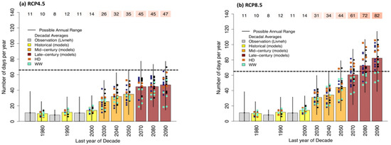
Figure 4.
Bar plot of decadal multi-model average climate model projections of the number of extreme heat (100 °F) days for (a) RCP4.5 and (b) RCP8.5. Different shading denotes observations, and the three reference periods. Range bars (thin vertical lines) depict the 5th–95th percentile of the spread of frequencies from each model/observation. Each marker denotes specific model projections for MACA (right, circles) and LOCA (left, squares) with HD and WW models shaded separately. The text values above each sub-panel show the multi-model mean number of extreme heat days for both SD methods, and the horizontal black line denotes the number of days observed in Oklahoma City during the 2011 heatwave and drought.
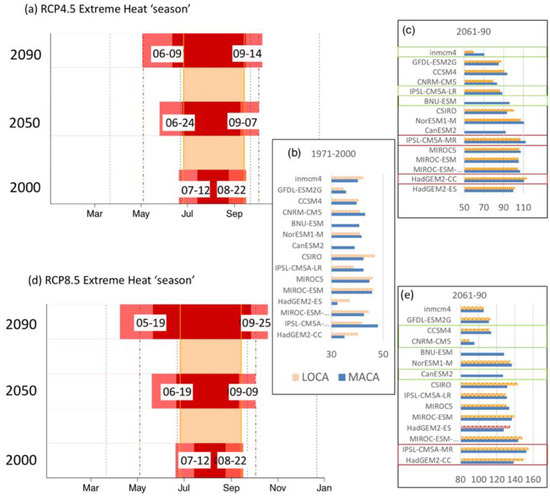
Figure 5.
Horizontal bar plot of CD5’s100 °F season for historical simulations (bottom bar plot in (a,d)) and future climate model projections (a) RCP4.5 and (d) RCP8.5. For (a,d), the y-axis is the 30-year period ending in the year shown. The red bar spans the multi-model average onset and end, with dates shown in text (month-day). The pink areas depict the model spread as the 5th percentile (onset date) and 95th percentile (end date). The shaded vertical box denotes the duration of the 2011 100 °F season for CD5, and the dashed-dot lines represent the average duration of the 100 °F season for present-day Phoenix, AZ, USA. The right panels show (b) the length of the 100 °F season (in days) for all models and SD datasets during the historical period, and the late 21st century for both (c) RCP4.5 and (e) RCP8.5. Green (red) boxes highlight the WW and HD models, respectively. Models are ordered by the magnitude of their average temperature increase between historical and late 21st century reference periods from smallest (top), to greatest change (bottom).
The 100 °F season lengthens through mid- and late-century, but the duration is substantially increased under RCP8.5 (Figure 5). Historically, extreme heat days are most common between mid-July and late August [40], and the historical SD projection agree with this observation (Figure 5a,d). Under RCP4.5 or by mid-century, the 100 °F season lasts from late June to early September; under RCP8.5, it lasts from late May to the end of September by late-century (Figure 5d), analogous to today’s climate of Phoenix, AZ. Earlier spring onset dominates the season lengthening. Again, differences between the two SD methods are apparent (Figure 5, right), but not particularly notable for most models and RCPs. Differences between HD and WW subsets (Figure 5b,c,e) relate to their temperature characteristics, with some of the largest increases in extreme heat season length in the HD subsets as greater increases in average temperatures increase the likelihood of more hot days and longer seasonal durations. This is further confirmed by displaying models in order of increasing mean temperature change (Figure 5b,c,e). We find high correlation between that metric and the 100 °F season for both emissions pathways (Pearson correlations ~0.85–0.90, not shown). Hotter temperatures in the region have historically been linked with more frequent or more intense drought conditions [42], due in part to enhanced soil moisture depletion through evapotranspiration [43,44] and changes in atmospheric circulation that favor warm season drying [45].
3.2. Winter Weather and Extreme Precipitation
3.2.1. Snow and Ice
Snow and ice (freezing rain and sleet) can be difficult to measure, and long-term records of precipitation type are typically restricted to ‘first-order’ National Weather Service stations situated in major cities [46]. For SD data, the temporal resolution and available surface variables prohibit distinguishing specific water phase types (e.g., snow, freezing rain) highlighted by survey respondents. Instead, we defined a proxy: winter precipitation of any phase occurs on a given day when daily Tmax ≤ 32 °F (0 °C) and precipitation >0.01 inch (0.25 mm). We estimated the frequency of winter weather occurrence using day counts from accumulated liquid water equivalent, hereafter LWE. This metric only approximates accumulation; a higher LWE implies more precipitation, although LWE cannot be equated with high confidence to an amount of ice accretion or snow accumulation [46]. Furthermore, daily temporal resolution likely results in an underestimate of LWE when maximum daily temperatures rise slightly above freezing.
Historically, central Oklahoma has, on average, four snow or ice days per year according to this proxy method, but with high interannual variability. Based on a study of precipitation phase types from Mullens and McPherson [42,46] using alternate data, there are approximately 0.75 ice days for every snow day. Snowfall dominates further north and west in the U.S. Southern Plains, whereas ice is proportionately the dominant phase type from southern Oklahoma into north and central Texas. Figure 6 shows projections under RCP4.5 (Figure 6a) and RCP8.5 (Figure 6c) for winter precipitation frequency as a time series normalized by the historical climatological frequency (1971–2000) as well as the projected change in intensity (amount per event)—accumulated LWE divided by event frequency—for select decadal periods (Figure 6b,d).
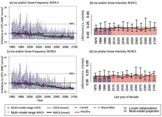
Figure 6.
Historical and future climate model projections in winter precipitation (ice/snow) days and intensity. Panels (a,c) are time series of the standardized winter precipitation (ice/snow) frequency (days) for RCP4.5, and RCP8.5, respectively, while panels (b,d) depict decadal mean changes winter precipitation intensity for RCP4.5 and RCP8.5, respectively, defined as total accumulated winter precipitation divided by the number of events. For (a,c), the thin black line is the multi-model mean, and the solid (stippled) shading is the 5th to 95th percentile range from all MACA (LOCA) models. Observed (Livneh) data are the thick dashed line, and the 5th–95th percentile values of the observed data (1971–2000) are shown by the horizontal thin dashed black lines. For panels (b,d), the range bars depict the 5th–95th percentile range from all models. Observations are overlaid for the historical period. HD and WW scenarios are shown in all plots by the solid and dashed lines, respectively.
Winter precipitation days for central Oklahoma are projected to decrease in frequency by approximately 30% (~1 day) by mid-century (Figure 6a,c) under both RCPs. Under RCP8.5 (RCP4.5) this frequency is expected to decrease by 80% (50%), or 3 (2) days, by the 2090s. Nonetheless, considerable year-to-year variability remains, and the projections’ spread infers the potential for years with above-normal winter weather frequency through 2050. Similarly, the projected intensity indicates that the average precipitation amount by event had no discernable change throughout the 21st century (Figure 6b,d). Thus, by late-century, snow and ice events across central Oklahoma under RCP8.5 are expected to be similar to the present-day frequency for north-central Texas (e.g., between Dallas and Austin)—i.e., approximately 1–2 ice or snow days per year. Based on historical phase climatology, this implies roughly two freezing precipitation (ice, sleet) events for every snowfall event [42]. Super-smoothed average HD and WW model projections show that winter precipitation reduces in frequency for HD by the mid-late century to a greater degree in RCP4.5 than RCP8.5. Under RCP8.5, there is little difference between HD and WW by late-century, and the subsets largely mirror the magnitude of the full ensemble. Furthermore, HD and WW subsets are indistinguishable for projected changes in intensity (Figure 6b,d).
3.2.2. Heavy Precipitation
Extreme precipitation events have been particularly salient hazards for Oklahoma in recent years. During 2010–2021, Oklahoma City had at least four precipitation days of ≥5 inches accumulation in 24 h, often resulting in urban flooding and loss of life. During 2015, excessive rainfall in May, June, and December produced repeated episodes of damaging floods throughout the state [42]. Studies have noted observed increases in the frequency of heavy precipitation for various regions of the United States [47,48,49]. Here, we assessed projected changes to extreme precipitation in central Oklahoma by calculating return periods of daily-accumulated rainfall over durations of 5–100 years, based on annual maxima and peaks-over-threshold (POT) sampling for extreme events over the three reference periods, using the methods of Mullens and McPherson [31]. Sub-daily intensity is a valued metric in hydrologic engineering; however, the daily resolution of the SD data did not permit investigations of sub-daily rain-rates.
The calculation of return-period frequency requires fitting an extreme value distribution (EVD) to the precipitation samples. EVD selection is non-trivial because different distributions produce different estimates, particularly at longer return intervals (>50 years) and when extrapolation is needed beyond the temporal range of the data. The Gumbel method [50], for example, can underestimate return magnitudes due to a shape parameter of zero, thereby reducing the weight of the extreme tails of the distribution [6]. In contrast, both the generalized extreme value (GEV) for annual maxima and generalized pareto (GP) for POT (here, the top 5% of daily precipitation) incorporate a shape parameter and focus on fitting the most ‘extreme’ extremes. Accurate estimates of extremely heavy precipitation are desirable, so long as the values are physically realistic. In the case of future projections, Mullens and McPherson [31] noted that magnitudes for MACA-derived return periods approached or even exceeded current probable maximum precipitation values in some locations, especially near the coastline. Although these issues were less apparent inland, outliers in our results should be interpreted with caution, as some models in combination with the SD approach produced aggressive increases in extreme precipitation magnitude that require further evaluation.
We examined both the GP and GEV distributions using the R package ‘ExtRemes’. As in Mullens and McPherson [31], both methods employed L-moments to model the distribution tail. Return periods for daily precipitation are shown for 5-, 10-, 20-, 50-, and 100-year intervals. Figure 7 shows the future change (average and 5th to 95th percentile spread) in the return period frequency in years, as an expression of how often a historical event of a certain return frequency could occur in the future. Figure 8 shows changes in the magnitude of future return-period accumulations compared with their historical values, based on all downscaled projections and the two EVDs. Generally, the Livneh observations (not shown) and SD multi-model average magnitudes for the 1-day return intervals scale similarly (within 1 inch) to those estimated from NOAA-Atlas 14 [51], with the largest discrepancy corresponding to the multi-model average of the LOCA projections, which underestimates magnitudes at the higher return periods (20–100 years, bottom of Figure 8).
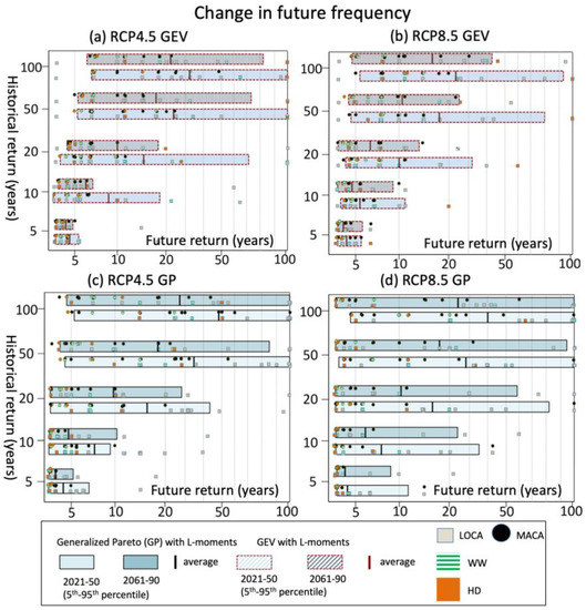
Figure 7.
Changes in the frequency of precipitation extremes at various return intervals. Panels (a,b) show results using GEV with annual maxima; panels (c,d) use GP with POT (top 5%). Shaded bars depict the 5th–95th percentile range in the projections, and the average by the vertical bar within each box. Values for individual projections include MACA (dots) and LOCA (squares), with HD and WW subsets shaded differently from the full ensemble. Return intervals were calculated over a range between 2 and 100 years. Values outside of this range were not estimated; therefore, any intervals that would have fallen outside of this range in the future period are not available.
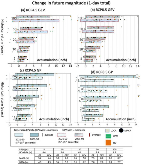
Figure 8.
As Figure 7, although here showing the change in return-period magnitudes (inches). The calculated historical return-period amounts (inches) for daily precipitation (table at bottom) show results for the two different EVDs and the NOAA-14 Atlas (observation/historical dataset).
Mid- and late-century projections from most downscaled GCMs show increases in the frequency of historically extreme precipitation, particularly under RCP8.5 (Figure 7a,b). LOCA and MACA differ in their representation of these extremes, where the sign of the change signal was sometimes opposite when downscaled by the same CMIP5 model, presumably based on how the SD method represents extreme precipitation. LOCA tends to produce a smaller change signal, and thus, less change in return period events (albeit still generally shorter in the future compared with the historical period). LOCA shows inconsistency in the direction of change in projections of extremes, which was noted in a recent study of the northeast United States by Wang et al. (2020) [52]. Supplementary Figure S5c identifies that the future LOCA distribution of the annual maxima has a shorter tail (hence, lower magnitude of extremes) compared with MACA. In contrast, MACA aggressively increases event frequencies, and the direction of change is consistent. However, the inter-model spread increases with larger return periods, as the EVD’s uncertainty grows with increased extrapolation. The GP’s spread is particularly large—possibly resulting from a larger sample (top 5% each year) of heavy precipitation events versus the climate-division annual maxima (one value per year). GP also shows several (not a majority) LOCA projections producing negative (i.e., lower intensity/frequency) future changes. Additionally, the variations in projections at this highly regional scale are more substantial than when data are aggregated over larger regions (e.g., compared with Mullens and McPherson [31]) because a heavier weight is placed on location-specific simulated extreme events.
Figure 8 mirrors these trends, showing the magnitudes of change between historical and future periods at various return intervals. RCP4.5 scenarios generally demonstrate lower average magnitude and frequency changes and less difference between the mid- and late-centuries, whereas RCP8.5 projections show increases in both future periods. The dominant effect on magnitude and frequency, however, appears to result from GCM differences (i.e., their physical representation of hydrologic processes), with substantial contributions from the selection of SD method or use of EVD, especially at the longest return intervals. When considering multi-projection averages from this sample, a historical 10-year rainfall event could occur 1.25–2.5 times more often in the mid-to-late-century, with the 50- and 100-year rainfall events projected to occur 2–5 times and 2–7 times more often, respectively. For average magnitudes, the 10-, 50, and 100-year return intervals increased by 0.9-2.8 inches (22.7–70.6 mm), 1.5–4.8 inches (37.8–121 mm), and 1.8–6.2 inches (45.4–156.2 mm), respectively, across all scenarios and future time periods. HD versus WW subsets show no preference for higher or lower values and no distinct differences from each other; they both occupy the middle to higher frequency and magnitude ranges. This result generally supports the view that changes in the magnitude of a model’s average temperature and precipitation in combination, or separately, are poorly related to changes in precipitation extremes [31]. In fact, there is no correlation (Pearson) between changes in magnitude of 100-year events and changes in average precipitation in late-century (not shown).
In aggregate, the magnitude and frequency of extreme precipitation events relative to the historical period increase substantially by mid-century. In other words, precipitation extremes are already under the influence of anthropogenic climate change. This assertion is further strengthened by observational evidence of recent, sustained increases in such extremes, posing an exacerbated hazard to transportation with time. Unfortunately, transportation design decisions become particularly challenging when considering model, SD, and EVD spread (Figure 7 and Figure 8) and associated uncertainty [7,21], continual updates of observational and model data, and the range of dataset choices. However, ensemble averages at least can provide more clarity on central tendencies. Based on these findings, a single or small subset of climate projections is not adequate to capture the range of plausible future extremes, leading to possible under- or over-design if used in planning [53].
4. Discussion
4.1. Contributions to Projection Spread
Throughout this analysis, we provide a general depiction of global climate model (GCM), downscaling method, and RCP scenario spread based on the choice of these three major contributors to resulting climate information. Here, we briefly summarize their relative contributions to the climate projections by estimating their associated variances as independently as possible (see the Supplementary Materials for a brief description of the approach). Figure 9 displays our findings. For this model, emissions and SD sample, the choice of GCM contributes most to the variance; thus, model selection is important. Too few GCMs or too many GCMs within the same model “family” may diminish the representativeness of the full range of future climates. Moreover, the use of climate subsets (“Hot/Dry”, “Warm/Wet”) in this study did not reflect a full range of future climates, so that technique for sub-setting data is not necessarily applicable to every region and variable and should be employed strategically. Temperature variables, particularly for heat, tended to show the least sensitivity to the downscaling data choices used in our analysis; thus, it may be acceptable to use one SD approach (MACA or LOCA) for this particular region and purpose. Nonetheless, caveats exist—including how SD methods deal with temporally sequenced events such as heatwaves. All variables are also bound by the ‘stationarity assumption’ that Dixon et al. (2016) [54] have identified as having distinct spatial variation in its applicability, with limits particularly in complex terrain and coastlines.
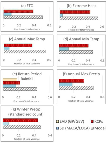
Figure 9.
Contributions of various aspects of a climate projection to total variance of each metric shown in (a–g). Model variance is the variance between model projections by the late 21st century using both RCP4.5 and RCP8.5, based on the MACA SD method only; emissions variance is the variance of the difference between late 21st century projections from RCP4.5 and RCP8.5; SD variance is the variance of the differences between MACA and LOCA simulations for all overlapping models. Lastly, extreme value distribution (EVD) variance is the difference between the 100-year return period magnitudes of daily precipitation (GP minus GEV) obtained for both future reference periods, and emissions scenarios. The plots show the fractional contributions of each variance type, with more details of this approach given in Supplementary Materials, Table S3.
We provide further evidence that magnitudes for extreme precipitation are distinctly influenced by the SD approach, as well as the EVD methods for extracting return periods, consistent with Mullens and McPherson [31], and reflected in other studies [52,55]. Wang et al. (2020) [52] also compared MACA and LOCA, finding greater differences between them for extremes than averages, with lower values of future relative change in LOCA, and especially so with the increasing ‘rareness’ of the extreme. They note that while there may be some contribution from training data, in instances where MACA and LOCA use the same training data (as in our study), method differences will dominate. For example, the temporal window over which relative precipitation changes are scaled (monthly in MACA, annually in LOCA) could affect the subsequent magnitudes. This finding highlights the necessity to carefully select GCMs and SD techniques when analyzing extreme precipitation, and to, when possible, leverage multiple options. Additional evidence is supplied through Supplementary Figure S5, which highlights some differences and similarities between LOCA and MACA distributions of many of the variables evaluated here
4.2. Transportation Implications
To summarize our results in a transportation-relevant context, we employed the ‘Sensitivity Matrix’ tool, developed from Rowan et al. [9], made available through the Federal Highway Administration. It qualitatively assesses the impacts of weather and climate ‘stressors’ on key types of transportation systems, infrastructure, and processes (‘assets’). We link projected trends in climate variables to transportation assets to create a sensitivity matrix, as shown in Figure 10. We assume that the future time periods are aligned well with the design life of the listed assets and that the asset is ostensibly new in the present time. For safety and maintenance operations, where decisions occur in the shorter term, we used the mid-century projection, which is similar between RCP4.5 and 8.5 for this region. For infrastructure with expected lifespans ≥50 years, we applied RCP8.5 end-of-century projections. We also assume that design paradigms and practices remain similar in the future as in the present, and assets have limited or no redundancy for climate-related impacts beyond their present-day expected frequency. ‘Confidence’ is based on the rubric of Mullens and McPherson [42]. This assessment is qualitative and only incorporates exposure as a risk measure, oversimplifying the role of climate-related stressors. Multiple alleviating or exacerbating stressors, such as asset age, construction quality, and traffic use, make climate-related vulnerability difficult to quantify independently and thoroughly [14].
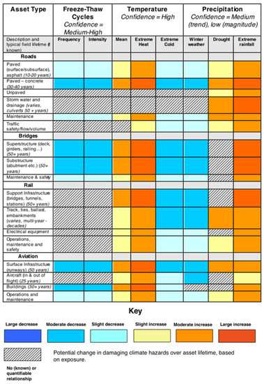
Figure 10.
‘Sensitivity Matrix’ for central Oklahoma, based on Rowan et al. [9] and available as a template through the resiliency toolkit of the U.S. Federal Highway Administration. The left column lists infrastructure assets and the shaded boxes denote the relative magnitude and direction of projected change associated with the climate criteria described in Section 4.2. Impact is therefore only a function of potential exposure to climate hazards. Diagonal hatching indicates unknown or negligible impacts. Confidence (top row) is based on the general framework from Mullens and McPherson [42] and is based on the availability of research and agreement among findings.
Some transportation assets could benefit from the reduction in cold season hazards. Fewer freeze-thaw cycles, cold extremes, and winter precipitation may reduce degradation to paved road and bridge surfaces, decreasing maintenance costs [56]. High annual variability in cold weather conditions, as evident in Figure 3 and Figure 6, means that these benefits are not universally true of all future years, one prescient example being that of February 2021, in which record-duration low temperatures were recorded in parts of Oklahoma and Texas [57]. Our greatest confidence exists with the projected trend in extreme heat (Figure 3, Figure 4 and Figure 5) and its impact on infrastructure, including increased risk of railroad track buckling, pavement buckling and rutting, and insufficient asphalt binders in some locations, particularly under load. As an example, Oklahoma currently uses binders ranging from PG64-22 to PG76-28. While some economic benefit is possible from reducing the low-temperature rating, projections indicate that binders with a hot temperature rating of less than 70 eventually will become unsuitable for the local climate (based on ratings for Phoenix, AZ, USA) [58]. Mallick et al. (2014) [59] estimated that expected pavement lifetimes could reduce by up to a factor of four nationally when incorporating climate change projections, especially increasing heat, and long-term increases in maintenance costs. Heat-related health hazards also contribute to adverse impacts on maintenance activities and scheduling. Heat extremes are anticipated to increase most substantially in the later 21st century, if emissions are not abated. In fact, based on our results, a road surfaced today could experience approximately double the number of days ≥100 °F (as compared with recent decades) by the end of its expected lifespan.
Ice and snow hazards to infrastructure are largely associated with coincident issues such as freeze–thaw cycles, cold temperatures, and the quantity and frequency of deicer use. Snow and ice days show decreases of up to 50–80% by late-century. Shorter-term activities (e.g., maintenance, safety, supply needs) may not experience much change in the near-term. Longer-term, moderate benefits to infrastructure, safety, and movement of transportation are expected, including economic benefit from fewer delays and less treating and removals of snow/ice. Nonetheless, projections for winter precipitation amounts indicate the continued potential for severe winter events, despite their lower frequency. Thus, transportation departments may not be as well-equipped or trained for these events when they do occur, an assertion that was explored by Bolinger et al. [57] in their discussion of the 2021 extreme winter weather in the U.S. Southern Plains.
Precipitation extremes, either extremely heavy rainfall or an extended lack of rainfall, are expected to increase. Increased heat coupled with similar or lower average precipitation, as demonstrated by Mullens and McPherson [31], can lead to more frequent or intense drought onset or persistence. Drought is primarily a concern for surface infrastructure in regions of expansive soils, including heavy clay soils in central Oklahoma, by promoting pavement and foundation damage when drought alternates with heavy rain (e.g., ‘shrink and swell’) [60]. Drought can also exacerbate blowing dust, a safety hazard across all modes of transportation [61].
We demonstrated an increasing trend in extreme rainfall for central Oklahoma, with the potential for a substantial change in return-period frequencies and magnitude by mid-century, regardless of emissions pathway. Our confidence in the precise magnitudes of change is low because values vary substantially across projections and EVDs. Nonetheless, the levels projected are potentially beyond the current redundancy of existing infrastructure. Infrastructure such as roadways, culverts/drainage, and bridges are sensitive to precipitation extremes, contributing to road and bridge scour, transportation disruption, and other damage [56].
5. Summary
This study details changes in transportation-relevant weather and climate variables for central Oklahoma using a large suite of statistically downscaled climate projections. Key variables and metrics were ascertained through expert input. The results are consistent with prior climate-science analyses (e.g., USGCRP 2018 [6], American Association of State Highway and Transportation Officials, FHWA, and DOT) regarding the direction of the trends in key variables; however, we provided specific regional quantitative information and assessment of uncertainties that are not found in the aforementioned resources.
This paper complements a growing body of research that focuses on identifying, planning, and adapting transportation systems to climate hazards [62]. As demonstrated by this study, the potential impacts of climate change are beneficial in some cases, but distinctly detrimental in others, and may necessitate the re-design, hardening, or paradigm shifts in aspects of transportation planning [22]. This research was regionally focused, and was limited by the lack of consistent collaboration between transportation and climate experts. Our stakeholder survey identified that while climate information is desired for many decisions, use of climate data outside of the community’s standard practice may be impractical and too resource-intensive (e.g., Appendix A, Figure A3). Ultimately, successful adaptations to the complexities of climate change will require increased communication and coproduction of information between the transportation and climate science communities [20,23].
Our study is part of a broader initiative to apply regional future climate projections across the South Central United States. State-by-state reports that detail transportation-relevant climate projections are available from the South Central Climate Adaptation Science Center (https://climateprojections.wixsite.com/transportation, date accessed on 1 July 2017). Transportation planners can use these reports as a scientific basis for understanding their regional’s changing climate and inform discussion over resilience and vulnerability in the South Central United States, as well as applying the techniques used here to examine climate change in the context of their planning needs.
Supplementary Materials
The following supporting information can be downloaded at: https://www.mdpi.com/article/10.3390/cli11020032/s1, Table S1: Climate data used in this study; Figure S1: MACA and LOCA climate scenario development; Table S2: Models in the hot-dry (HD) and warm-wet (WW) categories; Figure S2: Spatial temperature and precipitation changes 2061–2090 minus 1971–2000 using MACA; Figure S5: Same as Figure S3 but using LOCA; Figure S4: Historical freeze–thaw cycles derived from various datasets; Figure S6: Historical and late 21st century distributions of key variables from LOCA and MACA projections; Table S3: Description of methods used to estimate variance contributed by different factors of a climate projection [63].
Author Contributions
Conceptualization, E.M. and R.M.; methodology, E.M.; software, E.M.; validation, E.M.; formal analysis, E.M.; investigation, E.M. and R.M.; resources, E.M. and R.M.; data curation, E.M.; writing—original draft preparation, E.M.; writing—review and editing, E.M. and R.M.; visualization, E.M.; supervision, R.M.; project administration, E.M. and R.M.; funding acquisition, R.M. and E.M. All authors have read and agreed to the published version of the manuscript.
Funding
This study was supported by grants from the Southern Plains Transportation Center, University Strategic Organization, and NSF-EPSCoR under Grants SPTC-105336600, USO-122799700, and NSF OIA-1301789, respectively.
Data Availability Statement
Original data sources for Statistically Downscaled software are referenced in main text and acknowledgements. The majority of output data used for this work in NetCDF and text-file/csv format are available through the following portal: https://data.southcentralclimate.org/SPTC_Climate_Projections_Data_and_Images (assecced on 4 January 2023). For additional data requests, including anonymous survey data, please contact the corresponding author.
Acknowledgments
We would like to thank the survey participants for their insights, which informed the direction of research. Statistically downscaled climate data were courtesy of the MACA team at the University of Idaho, available from: http://www.climatologylab.org/maca.html (assecced on 4 January 2023), and the LOCA team from Scripps Institute, La Jolla, CA, USA, available from: http://climate.calcommons.org/ (assecced on 4 January 2023). We appreciate the scientific support of the USGS South Central Climate Adaptation Science Center, and the Southern Plains Transportation Center and its staff.
Conflicts of Interest
The authors declare no conflict of interest.
Appendix A
Weather and Climate Information Needs Survey
The detailed description of the survey and its findings can be found in Section 2.1 of McPherson and Mullens (2017), available at: http://www.sptc.org/projects (assecced on 4 January 2023) under SPTC14.1-50.
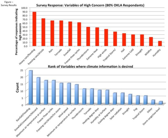
Figure A1.
Ranks of weather/climate variables of concern (top; percentage of responses indicating high concern) and information need (bottom; number of participants who selected listed options) drawn from survey responses. Participants could select multiple answers.

Figure A2.
Thresholds demarking adverse temperatures based on survey responses. The size of the number is proportional to the number of times it was referenced. From Figure 3 of [31].
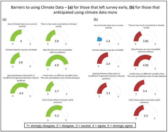
Figure A3.
Average response on a Likert scale (1 = strongly disagree, 3 = neutral, 5 = strongly agree) from survey respondents’ regarding their perceptions of barriers to using climate data (inclusive of historical and future data). Responses include those who exited the full survey early (green, left, n = 7), and those who completed the full survey (red, right, average n = 27). The level of agreement between the two categories differs notably for some aspects of this query (e.g., those who do plan to use climate data also show it to not be a priority). Respondents in both categories, however, agreed with statements such as: “I need more, or different variables from ones provided by most climate datasets” and “spacing between data-points is insufficient to generate decision-relevant guidance.” While addressing these limitations was beyond the project scope, it may be useful to readers to consider some of the problems with the uptake of climate data as mentioned by these stakeholders.
References
- Liu, A.; Soneja, S.I.; Jiang, C.; Huang, C.; Kerns, T.; Beck, K.; Mitchell, K.; Sapkota, A. Frequency of extreme weather events and increased risk of motor vehicle collision in Maryland. Sci. Total Environ. 2017, 580, 550–555. [Google Scholar] [CrossRef]
- Black, A.W.; Mote, T.L. Characteristics of Winter Precipitation Related Transportation Fatalities in the United States. Wea. Clim. Soc. 2015, 7, 133–145. [Google Scholar] [CrossRef]
- Markolf, S.; Luskova, M. Transportation resilience to climate change and extreme weather events-Beyond risk and robustness. Transp. Policy 2019, 74, 174–186. [Google Scholar] [CrossRef]
- Venner, M.; Zamurs, J. Increased Maintenance Coasts of Extreme Weather Events. Transp. Res. Board. J. Transp. Res. Board 2012, 2292, 20–28. [Google Scholar] [CrossRef]
- Neumann, J.; Chinowsky, P.; Helman, J.; Black, M.; Fant, C.; Strzepek, K.; Martinich, J. Climate effects on US infrastructure: The economics of adaptation for rail, roads, and coastal development. Clim. Chang. 2021, 167, 44. [Google Scholar] [CrossRef] [PubMed]
- Reidmiller, D.R.; Avery, C.W.; Easterling, D.R.; Kunkel, K.E.; Lewis, K.L.; Maycock, T.K.; Stewart, B.C. Impacts, Risks, and Adaptation in the United States: Fourth National Climate Assessment, Volume II; U.S. Global Change Research Program: Washington, DC, USA, 2018. [Google Scholar] [CrossRef]
- Hayhoe, K.; Stoner, A.; Abeysundara, S.; Daniel, J.S.; Jacobs, J.M.; Kirshen, P.; Benestad, R. Climate projections for transportation infrastructure planning, operations and maintenance, and design. Transp. Res. Rec. J. Transp. Res. Board 2015, 2510, 90–97. [Google Scholar] [CrossRef]
- National Academies of Science, Engineering, and Medicine Transportation Research Board. Applying Climate Change Information to Hydrologic and Hydraulic Design of Transportation Infrastructure. 2019. Available online: https://apps.trb.org/cmsfeed/TRBNetProjectDisplay.asp?ProjectID=4046 (accessed on 11 January 2022).
- Rowan, E.; Evans, C.; Riley-Gilbert, M.; Hyman, R.; Kafalenos, R.; Beucler, B.; Rodehorst, B.; Choate, A.; Schultz, P. Assessing the sensitivity of transportation assets to extreme weather events and climate change. Transp. Res. Board J. Transp. Res. Board 2013, 2326, 16–23. [Google Scholar] [CrossRef]
- Rowan, E.; Snow, C.; Choate, A.; Rodehurst, B.; Asam, S.; Hyman, R.; Kafalenos, R.; Gye, A. Indicator Approach for Assessing Climate Change Vulnerability in Transportation Infrastructure. Transp. Res. Board J. Transp. Res. Board 2014, 2459, 18–28. [Google Scholar] [CrossRef]
- Vajda, A.; Tuomenvirta, H.; Jokinen, P. Observed and Future Changes of Extreme Winter Events in Europe with Implications for Transportation. In Proceedings of the SIWEC ID0040, Helsinki, Finland, 22–25 May 2012; p. 8. Available online: http://www.sirwec.org/Papers/helsinki/40.pdf (accessed on 1 April 2018).
- Melvin, A.; Larson, P.; Boehlert, B.; Neumann, J.E.; Chinowsky, P.; Espinet, X.; Martinich, J.; Baumann, M.S.; Rennels, L.; Bothner, A.; et al. Climate Damages to Alaska Public Infrastructure. Proc. Natl. Acad. Sci. USA 2017, 114, 122–131. [Google Scholar] [CrossRef]
- Winguth, A.; Lee, J.H.; Ko, Y.; UTA, and North Central Texas Vulnerability Assessment Team. Climate Change/Extreme Weather Vulnerability and Risk Assessment for Transportation Infrastructure in Dallas and Tarrant Counties. Fed. Highw. Adm. 2015, 52. Available online: https://www.fhwa.dot.gov/environment/sustainability/resilience/pilots/2013-2015_pilots/nctcog/final_report/nctogfinal.pdf (accessed on 1 June 2017).
- CAMPO. Central Texas Extreme Weather and Climate Change Vulnerability Assessment of Regional Transportation Infrastructure. Final Report. Fed. Highw. Adm. Camb. Syst. Inc. 2015, 220. Available online: https://www.fhwa.dot.gov/environment/sustainability/resilience/pilots/2013-2015_pilots/campo/final_report/index.cfm (accessed on 1 June 2017).
- ASCE (American Society of Civil Engineers). Report Card for Oklahoma’s Infrastructure. 2013. Available online: https://www.infrastructurereportcard.org/wp-content/uploads/2016/10/ASCE-OK-2013-Report-Card.pdf (accessed on 1 August 2017).
- ASCE. Report Card for America’ Infrastructure: Oklahoma Infrastructure. 2021. Available online: https://infrastructurereportcard.org/state-item/oklahoma/ (accessed on 9 October 2022).
- Oklahoma Dept. Transportation (ODOT). 2015-40 Oklahoma Long Range Transportation Plan: Moving Oklahoma Forward. 2015. Available online: http://www.okladot.state.ok.us/p-r-div/lrp_2015_2040/2040_LRTP_Full_Document.pdf (accessed on 2 May 2018).
- Asam, S.; Bhat, C.; Dix, B.; Bauer, J.; Gopalakrishna, D. Climate Change Adaptation Guide for Transportation Systems Management, Operations, and Maintenance; U.S. Department of Transportation: Washington, DC, USA, 2015; p. 86. Available online: https://ops.fhwa.dot.gov/publications/fhwahop15026/fhwahop15026.pdf (accessed on 1 June 2017).
- Choate, A.; Dix, B.; Rodehorst, B.; Wong, A.; Jaglom, W.; Keller, J.; Lennon, J.; Dorney, C.; Kuchibhotla, R.; Jagannath, M.; et al. Synthesis of Approaches for Addressing Resilience in Project Development; Federal Highways Administration Technical Report FHWA-HEP-17-082; Federal Highways Administration: Washington, DC, USA, 2017; p. 224. Available online: https://www.fhwa.dot.gov/environment/sustainability/resilience/ongoing_and_current_research/teacr/synthesis/fhwahep17082.pdf (accessed on 1 April 2018).
- Meyer, M.D.; Rowan, E.; Snow, C.; Choate, A. Impacts of Extreme Weather on Transportation: National Symposium Summary; ICF International: Roston, VA, USA, 2013; Available online: https://climatechange.transportation.org/pdf/2013_symposium/AASHTO_EWESymposium_2013.pdf (accessed on 21 July 2022).
- Douglas, E.; Jacobs, J.; Hayhoe, K.; Silka, L.; Daniel, J.; Collins, M.; Alipour, A.; Anderson, B.; Hebson, C.; Mecray, E.; et al. Progress and Challenges in Incorporating Climate Change Information into Transportation Research and Design. J. Infrastruct. Syst. 2017, 23, 9. [Google Scholar] [CrossRef]
- Quinn, A.D.; Ferranti, E.S.; Hodgkinson, S.P.; Jack, A.R.; Beckgord, J.; Dora, J.M. Adaptation becoming Business-as-Usual: A Framework for Climate Change Ready Transportation Infrastructure. Infrastructures 2018, 3, 10. [Google Scholar] [CrossRef]
- McPherson, R.A.; Mullens, E.D. Trends in Cold Extremes and Winter Weather for the SPTC Region. South. Plains Transp. Cent. Final Rep. 2017, 131. Available online: http://www.sptc.org/projects/ (accessed on 4 January 2023).
- Wang, S.-Y.; Huang, W.-R.; Hsu, H.-H.; Gillies, R.R. Role of the strengthened El Niño teleconnection in the May 2015 floods over the southern Great Plains. Geophys. Res. Lett. 2015, 42, 8140–8146. [Google Scholar] [CrossRef]
- VanBuskirk, O.; Ćwik, P.; McPherson, R.A.; Lazrus, H.; Martin, E.; Kuster, C.; Mullens, E. Listening to Stakeholders: Initiating Research on Sub-seasonal to Seasonal Heavy Precipitation Events in the Contiguous, U.S. by First Understanding What Stakeholders Need. Bull. Am. Meteorol. Soc. 2021, 102, E1972–E1986. Available online: https://journals.ametsoc.org/view/journals/bams/aop/BAMS-D-20-0313.1/BAMS-D-20-0313.1.xml (accessed on 4 January 2023). [CrossRef]
- Gutiérrez, J.M.; San-Martín, D.; Brands, S.; Manzanas, R.; Herrera, S. Reassessing Statistical Downscaling Techniques for Their Robust Application under Climate Change Conditions. J. Clim. 2013, 26, 171–188. [Google Scholar] [CrossRef]
- Abatzoglou, J.T.; Brown, T.J. A comparison of statistical downscaling methods suited for wildfire applications. Int. J. Climatol. 2012, 32, 772–780. [Google Scholar] [CrossRef]
- Pierce, D.W.; Cayan, D.R.; Thrasher, B.L. Statistical Downscaling Using Localized Constructed Analogs (LOCA). J. Hydrometeor. 2014, 15, 2558–2585. [Google Scholar] [CrossRef]
- Taylor, K.E.; Stouffer, R.J.; Meehl, G.A. An Overview of CMIP5 and the Experiment Design. Bull. Amer. Meteor. Soc. 2012, 93, 485–498. [Google Scholar] [CrossRef]
- Livneh, B.; Rosenburg, E.A.; Lin, C.; Nijssen, B.; Mishra, V.; Andreadis, K.M.; Maurer, E.; Lettenmaier, D.P. A Long-Term Hydrologically Based Dataset of Land Surface Fluxes and States for the Conterminous United States: Update and Extensions. J. Clim. 2013, 26, 9384–9392. [Google Scholar] [CrossRef]
- Mullens, E.D.; McPherson, R.A. Quantitative scenarios for future hydrologic extremes in the U.S. Southern Great Plains. Int. J. Climatol. 2019, 39, 2659–2676. [Google Scholar] [CrossRef]
- Van Vuuren, D.P.; Carter, T.R. Climate and Socio-economic Scenarios for Climate Change Research and Assessment: Reconciling the new with the old. Clim. Chang. 2013, 122, 415–429. [Google Scholar] [CrossRef]
- Pierce, D.W.; Cayan, D.R.; Maurer, E.P.; Abatzoglou, J.T.; Hegewisch, K.C. Improved Bias Correction Techniques for Hydrological Simulations of Climate Change. J. Hydrometeor. 2015, 16, 2421–2442. [Google Scholar] [CrossRef]
- Oklahoma Dept. Transportation (ODOT). 8-Year Construction Work Plan. 2017. Available online: https://www.ok.gov/odot/Programs_and_Projects/8_Year_Construction_Work_Plan/ (accessed on 1 June 2017).
- Guttman, N.B.; Quayle, R.G. A historical perspective of US climate divisions. Bull. Am. Meteorol. Soc. 1996, 77, 293–303. [Google Scholar] [CrossRef]
- Hershfield, D.M. The Frequency of Freeze-Thaw Cycles. J. Appl. Meteor. 1974, 13, 348–354. [Google Scholar] [CrossRef]
- Haley, J.S. Climatology of Freeze-Thaw Days in the Conterminous United States: 1982–2009. Master’s Thesis, Kent State University, Kent, OH, USA, 2011. Available online: https://etd.ohiolink.edu/!etd.send_file?accession=kent1302547210&disposition=inline (accessed on 1 February 2015).
- Friedman, J.H. A Variable Span Smoother; Technical Report (5); Laboratory for Computational Statistics, Department of Statistics, Stanford University: Stanford, CA, USA, 1984. [Google Scholar]
- McPherson, R.A.; Fiebrich, C.; Crawford, K.C.; Elliott, R.L.; Kilby, J.R.; Grimsley, D.L.; Martinez, J.E.; Basara, J.B.; Illston, B.G.; Morris, D.A.; et al. Shrivastava, 2007: Statewide monitoring of the mesoscale environment: A technical update on the Oklahoma Mesonet. J. Atmos. Oceanic Technol. 2007, 24, 301–321. [Google Scholar] [CrossRef]
- National Weather Service (NWS) Norman. Quick Hot Temperature Facts for Oklahoma City, OK (Since 1891). 2012. Available online: http://www.crh.noaa.gov/oun/?n=summertimetemp_facts_okc (accessed on 1 August 2017).
- National Weather Service (NWS) Phoenix. When Does the First and Last 100 °F Day Typically Occur? 2016. Available online: https://www.wrh.noaa.gov/psr/climate/FirstLastHeatDays.php (accessed on 1 June 2018).
- Mullens, E.D.; McPherson, R.A. Oklahoma: A weather and climate trends roadmap. South Cent. Clim. Sci. Cent. Norman OK 2017, 35. Available online: https://climateprojections.wixsite.com/transportation/oklahoma (accessed on 4 January 2023).
- Williams, A.P.; Seager, R.; Abatzoglou, J.T.; Cook, B.I.; Smerdon, J.E.; Cook, E.R. Contribution of anthropogenic warming to California drought during 2012–2014. Geophys. Res. Lett. 2015, 42, 6819–6828. [Google Scholar] [CrossRef]
- Cowan, T.; Hegerl, G.C.; Colfescu, I.; Bollasina, M.; Purich, A.; Boschat, G. Factors contributing to record-breaking heat waves over the Great Plains during the 1930s Dust Bowl. J. Clim. 2017, 30, 2437–2461. [Google Scholar] [CrossRef]
- Ryu, J.H.; Hayhoe, K. Observed and CMIP5 modeled influence of large-scale circulation on summer precipitation and drought in the South-Central United States. Clim. Dyn. 2017, 49, 4293–4310. [Google Scholar] [CrossRef]
- Mullens, E.D.; McPherson, R.A. A Multi-Algorithm Reanalysis-based Freezing Precipitation Dataset for Climate Studies in the South-Central US. J. Appl. Meteorol. Clim. 2017, 56, 495–517. [Google Scholar] [CrossRef]
- Mullens, E.D.; Hocker, J.; Shafer, M. Trends in Heavy Precipitation in the Southern USA. Weather 2013, 68, 311–316. [Google Scholar] [CrossRef]
- Kunkel, K.E.; Karl, T.R.; Brooks, H.; Kossin, J.; Lawrimore, J.H.; Arndt, D.; Bosart, L.F.; Changnon, D.; Cutter, S.; Doesken, N.J.; et al. Monitoring and Understanding Trends in Extreme Storms: State of Knowledge. Bull. Amer. Meteor. Soc. 2013, 94, 499–514. [Google Scholar] [CrossRef]
- Powell, E.J.; Keim, B.D. Trends in Daily Temperature and Precipitation Extremes for the Southeastern United States: 1948–2012. J. Clim. 2015, 28, 1592–1612. [Google Scholar] [CrossRef]
- Gumbel, E.J. Statistics of Extremes; Columbia University Press: New York, NY, USA, 1958. [Google Scholar]
- Perica, S.; Martin, D.; Pavlovic, S.; Roy, I.; Laurent, M.S.; Trypaluk, C.; Unruh, D.; Yekta, M.; Bonnin, G. NOAA Atlas 14—Frequency Atlas of the United States (Midwestern States). 2013. Available online: http://www.nws.noaa.gov/oh/hdsc/PF_documents/Atlas14_Volume8.pdf (accessed on 1 July 2017).
- Wang, G.; Kirchhoff, C.; Seth, A.; Abatzoglou, J.T.; Livneh, B.; Pierce, D.W.; Fomenko, L.; Ding, T. Projected Changes of Precipitation Characteristics Depend on Downscaling Method and Training Data: MACA vs. LOCA using the U.S. Northeast as an Example. J. Hydrometeor. 2015, 21, 2739–2758. [Google Scholar] [CrossRef]
- Lopez-Cantu, T.; Prein, A.F.; Samaras, C. Uncertainties in US Extreme Precipitation from Downscaled Climate Projections. Geophys. Res. Lett. 2020, 47, 11. [Google Scholar] [CrossRef]
- Dixon, K.W.; Lanzante, J.R.; Nath, M.J.; Hayhoe, K.; Stoner, A.; Radhakrishnan, A.; Balaji, V.; Gaitán, C.F. Evaluating the stationarity assumption in statistically downscaled climate projections: Is past performance an indicator of future results? Clim. Chang. 2016, 135, 395–408. [Google Scholar] [CrossRef]
- Alder, J.R.; Hostetler, S.W. The Dependence of Hydroclimate Projections in Snow-Dominated regions of the Western United States on the Choice of Statistically Downscaled Climate Data. Water Resour. Res. 2019, 55, 2279–2300. [Google Scholar] [CrossRef]
- Neumann, J.E.; Price, J.; Chinowsky, P.; Wright, L.; Ludwig, L.; Streeter, R.; Jones, R.; Smith, J.B.; Perkins, W.; Jantarasami, L.; et al. Climate change risks to US Infrastructure: Impacts on Roads, Bridges, Coastal Development, and Urban Drainage. Clim. Chang. 2014, 131, 97–109. [Google Scholar] [CrossRef]
- Bolinger, R.A.; Brown, V.M.; Fuhrmann, C.M.; Gleason, K.L.; Andrew Joyner, T.; Keim, B.D.; Lewis, A.; Nielsen-Gammon, J.; Stiles, C.J.; Tollefson, W.; et al. An assessment of the extremes and impacts of the February 2021 South-Central, U.S Arctic outbreak, and how climate services can help. Weather Clim. Extrem. 2022, 36, 17. [Google Scholar] [CrossRef]
- Yavuzturk, C.; Ksaibati, K. Assessment of Temperature Fluctuations in Asphalt Pavements due to Thermal Environmental Conditions using a Two-Dimensional Transient Finite Difference Approach. Transp. Res. Board MPC Rep. No. 02-136 2002, 17, 465–475. [Google Scholar] [CrossRef]
- Mallick, R.B.; Radzicki, M.J.; Daniel, J.S.; Jacobs, J.M. Use of system dynamics to understand the long term impact of climate change on pavement performance and maintenance cost. Transp. Res. Board J. Transp. Res. Board 2014, 2455, 1–9. [Google Scholar] [CrossRef]
- Carter, B.J.; Gregory, M.S. Soil Map of Oklahoma. Okla. Geol. Surv. Educ. Publ. 2008, 9, 16–20. Available online: http://www.ogs.ou.edu/pubsscanned/EP9p16_19soil_veg_cl.pdf (accessed on 1 August 2017).
- Ashley, W.S.; Strader, S.; Dziubla, D.C.; Haberlie, A. Driving Blind: Weather-Related Vision Hazards and Fatal Motor Vehicle Crashes. Bull. Amer. Meteor. Soc. 2015, 96, 755–778. [Google Scholar] [CrossRef]
- ICF International. 2013–2015 Climate Resilience Pilot Program: Outcomes, Lessons Learned, and Recommendations; Technical Report FHWA-HEP-16-079; Federal Highway Administration: Washington, DC, USA, 2016; p. 58. Available online: https://www.fhwa.dot.gov/environment/sustainability/resilience/pilots/2013-2015_pilots/final_report/fhwahep16079.pdf (accessed on 1 August 2017).
- Maurer, E.P.; Hidalgo, H.G.; Das, T.; Dettinger, M.D.; Cayan, D.R. The utility of daily large-scale climate data in the assessment of climate change impacts on daily streamflow in California. Hydrol. Earth Syst. Sci. 2010, 14, 1125–1138. [Google Scholar] [CrossRef]
Disclaimer/Publisher’s Note: The statements, opinions and data contained in all publications are solely those of the individual author(s) and contributor(s) and not of MDPI and/or the editor(s). MDPI and/or the editor(s) disclaim responsibility for any injury to people or property resulting from any ideas, methods, instructions or products referred to in the content. |
© 2023 by the authors. Licensee MDPI, Basel, Switzerland. This article is an open access article distributed under the terms and conditions of the Creative Commons Attribution (CC BY) license (https://creativecommons.org/licenses/by/4.0/).