Impact of Blue Space Geometry on Urban Heat Island Mitigation

Abstract

A growing body of literature recognises the importance of nature-based solutions in providing resilience to the effects of climate change by mitigating urban heat islands. However, a knowledge gap exists regarding the contribution of blue spaces to the urban environment. Recent evidence suggests that blue spaces within urban canyons can promote pollutant removal via the vertical transport of air under certain conditions, but this is inconclusive. Using a numerical solver that accounts for evaporation effects, we investigate the influence of blue space size and shape on the in-canyon flow structure, temperature and water vapour distribution. Simulations were performed for water bodies of varying size and shape at different temperatures compared to the surrounding air. Results suggest that inadequately sized warmer water bodies are unable to promote sufficient vertical transport for pollutant removal, leading to overturning and increased temperature and humidity levels at the pedestrian level, thereby worsening environmental conditions and increasing the risk of heat-related illness and mortality. Hence, larger water bodies are better suited to nocturnal transport of pollutants and accumulated warm air away from the urban surface, while smaller water bodies are better suited to providing localised evaporative cooling. Lastly, irregular water bodies may have a greater cooling effect across a larger area.

1. Introduction

Extreme heat and high temperatures have become more frequent and more intense across most land regions and are projected to continue to worsen as a result of climate change [1,2]. For instance, the recent 2022 UK heat wave that saw record-breaking temperatures of over 40 °C in the country was a glimpse of the future. Over the last two decades, there have been approximately 800 heat-related deaths per year on average in England and Wales [3]. It is estimated that by 2050, heat-related deaths will reach 7000 per annum across the UK [4]. This increased risk of heat stress is and will continue to be even more pronounced in cities, which are known to exhibit their own climate, typically being warmer than their rural surroundings, a phenomenon known as Urban Heat Island (UHI) [5]. The UHI can be likened to a bubble of air situated over a city, isolated from the rest of the atmosphere and typified by decreased vertical transport of air, trapping warm air and pollutants in the lower part of the atmospheric boundary layer (i.e., at street level), which poses another major health threat. More frequent and intense heat waves typified by hotter days and warmer nights will exacerbate the effects of the UHI on public health.

Nature-based solutions (NBS)—actions inspired by, supported by, or copied from nature—have emerged as a powerful tool to address climate change and biodiversity loss while at the same time enhancing citizen well-being [6,7]. The ability of NBS such as urban green (e.g., city parks, avenue and roadside trees and green roofs) and blue spaces (e.g. water channels, urban lakes, ponds and rivers) to increase evapotranspiration and, thus, promote vertical transport of heat, air and pollutants has led to NBS being touted as a way to mitigate the UHI. However, the mechanisms that underpin blue NBS performance are not fully understood, as the focus of recent advances in NBS has been almost exclusively directed towards green NBS [8,9].

Despite the insight provided by the existing range of studies, which include field measurements, numerical simulations and remote sensing, there are significant discrepancies between the methods, the parameters considered, and the meteorological conditions under which each study is carried out [8]. To date, computational fluid dynamics (CFD) studies on urban blue spaces have been limited, and they often ignore evaporation effects and the impact on airflow. This is mainly due to the inherently complex nature of evaporation phenomena and the lack of consistent approaches to evaporation modelling and accurate numerical solvers. In addition, there are no available benchmark cases of water bodies within urban areas to use for validation studies to attract research attention. This has resulted in uncertainties regarding the magnitude of blue spaces’ mitigating potential and the influence of factors such as size and shape. There is also a lack of information about how the diurnal and seasonal variability of the atmospheric structures and processes above blue spaces affect their thermal interactions with the surrounding environment [8].

Much of the current literature on the influence of blue space size focuses on thermal comfort effects and the cooling potential it offers to the surrounding urban environment. For instance, Syafii et al. [10] experimentally studied how various water body configurations influenced their thermal behaviour in an outdoor scale model. Their results suggested that the greater the water surface area, the more significant the cooling effect, i.e., the air temperature drop at a point location above the water body relative to a reference point within a street canyon without water bodies. A remote sensing study conducted by Sun and Chen [11] found that larger water bodies offer greater cooling intensity (°C/hm), meaning greater land surface temperature drop per distance from the water body. However, when the water body area was used to estimate the cooling efficiency (°C/hm/ha), they showed that several smaller water bodies of the same total area offer more beneficial effects. A numerical modelling study by Theeuwes et al. [12] corroborated the findings of Sun and Chen [11] by simulating blue space effects in an idealised circular city using the mesoscale Weather Research and Forecasting (WRF) model. The authors found that a large blue space presents a strong cooling effect on its surroundings, whilst smaller water bodies of a total equivalent area influence a broader city area. Other studies have highlighted the importance of the blue space area coverage ratio in terms of its effect on human heat stress. For instance, Zhao and Fong [13,14] suggested that a blue space can improve thermal comfort conditions only if it covers more than 34% of the domain, whereas if they cover a smaller area, the cooling effects are insufficient to compensate for the increased humidity that worsens thermal comfort.

The landscape shape index ($LSI$) is the parameter that often appears in the existing research with regards to blue space shape and is defined as:

$$LSI=\frac{P_t}{2\times \sqrt{\pi A}},$$

(1)

where $P_t$ is the total perimeter, and A is the area of the water body. Therefore, a circular water body would have an $LSI$ of one. A few studies agree that the rounder the water body, i.e., small $LSI$ values, the greater the temperature decrease compared to the urban surroundings [11,15,16]. In addition, some researchers have suggested that narrow blue spaces create a weak humidity and temperature gradient with the surrounding built-up area, and therefore, a width threshold must exist in order to maintain their cooling effects [11,17]. This interpretation differs from that of Du et al. [18] and Xue et al. [19] who argue that irregular water bodies with higher $LSI$ values offer greater cooling potential as their larger perimeter leads to increased heat exchange with their urban surroundings. Tan et al. [20] also suggested that the more complex the shape of a blue space is, the larger its influencing area. In a remote sensing study conducted for Copenhagen, Yang et al. [21] found that when blue spaces were smaller than 1 ha, compact sizes (low $LSI$) led to better cooling, whereas when the size was larger than 1 ha, a more complex shape seemed to provide better cooling effects. Those rather contradictory findings may be due to the fact that researchers tend to overlook the impact of the background atmospheric conditions on the overall blue space performance. For instance, does the prevailing wind have the same direction over the blue spaces under examination? Is part or all of the water surface exposed or obstructed by the prevailing wind? Is the attempted comparison quantified by normalising against varied air–water temperature differences?

CFD is an ideal tool to investigate these factors and carefully assess blue space thermal interactions with the built environment under controlled conditions. This study extends the work conducted by Ampatzidis et al. [22] by offering critical insights into the influence of blue space size and shape on the in-canyon dynamics and flow structure within an idealised urban neighbourhood under neutral atmospheric conditions. Cases with cooler (daytime—spring/early summer) and warmer water bodies (nighttime—late summer) under a mixed convection regime are also considered. The reference temperature difference between the water surface and the surrounding air is constant at $\Delta T_0=\pm 2$ K.

This study contributes to the growing research area of urban blue spaces through exploring how the geometry of a blue space impacts the thermal interaction with the surrounding urban environment. The novelty of this study is threefold: first, the employed in-house solver reproduces the complex phenomenon of evaporation accounting for heat exchange; second, the adaptation of the model for RANS modelling allows the investigation of complex urban configurations under realistic conditions, i.e., with high Reynolds and Richardson numbers; and finally, the employment of different air–water temperature differences as a proxy for different parts of the diurnal cycle and different seasons allows the assessment of blue spaces for practical applications.

2. Materials and Methods

2.1. Governing Equations

Ambient air is considered a mixture of ideal gases, air and water vapour and is modelled as an incompressible and viscous Newtonian fluid. The onset of buoyancy forces is taken into account via the Boussinesq approximation and is induced by temperature (T [K]) and vapour concentration ($\omega$ [–]) gradients. In this framework, the governing equations read:

$$\begin{array}{cc}\hfill & \frac{\partial u_j}{\partial x_j}=0,\hfill \end{array}$$

(2)

$$\begin{array}{cc}\hfill & \frac{\partial u_i}{\partial t}+\frac{\partial u_j{u}_i}{\partial x_j}=-\frac{1}{{\rho }_0}\frac{\partial p}{\partial x_i}+\nu \frac{{\partial }^2{u}_i}{\partial x_j\partial x_j}+b_i,\hfill \end{array}$$

(3)

$$\begin{array}{cc}\hfill & b_i=g_i\left(1-{\beta }_T\Delta T-{\beta }_{\omega }\Delta \omega \right),\hfill \end{array}$$

(4)

where $u_i$ is the velocity component in the $x_i$ direction [ms${}^{-1}$], p is the pressure [Pa], ${\rho }_0$ is the reference fluid density [kg m${}^{-3}$], $\nu$ is the molecular kinematic viscosity [m²s⁻¹], $b_i$ is the buoyancy force [ms${}^{-2}$], and $g_i$ is the gravitational acceleration [ms${}^{-2}$]. Buoyancy is expressed in terms of variation of temperature $\Delta T$ and vapour concentration $\Delta \omega$ with respect to reference values and their volume expansion coefficients ${\beta }_T$ [K${}^{-1}$] and ${\beta }_{\omega }$ [–]. The equations for temperature and water vapour read:

$$\begin{array}{cc}\hfill & \frac{\partial T}{\partial t}+\frac{\partial }{\partial x_j}\left(T{u}_i\right)-{\alpha }_T\frac{{\partial }^{2}T}{\partial x_k\partial x_k}=S_e,\hfill \end{array}$$

(5)

$$\begin{array}{cc}\hfill & \frac{\partial \omega }{\partial t}+\frac{\partial }{\partial x_j}\left(\omega u_i\right)-{\alpha }_{\omega }\frac{{\partial }^2\omega }{\partial x_k\partial x_k}=0,\hfill \end{array}$$

(6)

where ${\alpha }_T$ and ${\alpha }_{\omega }$ are the molecular and turbulent diffusivities of air and water vapour, respectively, and $S_e$ is the evaporation heat sink term.

2.2. Evaporation Model

This study adopts the evaporation model proposed in Cintolesi et al. [23,24] and adapted to RANS simulations by Ampatzidis et al. [22]. The blue space is considered at rest and isothermal. Hence, the reproduction of the internal motions of water is out of the scope of this study. Instead, the blue space is modelled through the thin-film assumption, meaning that water is approximated as a wet surface that can evaporate infinitely, acting as a constant source of water vapour [25]. This model is applied as a set of boundary conditions at the water surface.

A semi-impermeable model [26] is employed to model the evaporation velocity $u_{\omega }$ that is dependent on the water vapour gradient in the direction normal to the water surface:

$$u_{\omega ,i}=-\frac{{\alpha }_{\omega }}{1-{\omega }_{\mathsf{\Gamma }}}\left(\frac{d\omega }{d{n}_i}{|}_{\mathsf{\Gamma }}\right)n_i,$$

(7)

where the subscript $\mathsf{\Gamma }$ indicates that the quantities are evaluated at the air–water interface, and $n_i$ is the vector normal to the interface pointing into the domain. The vapour concentration at the interface is computed as in [23] by the following empirical formula:

$${\omega }_{\mathsf{\Gamma }}=\frac{M_v}{M_a}\frac{{\varphi }_{\mathsf{\Gamma }}{p}_{sat}\left(T_{\mathsf{\Gamma }}\right)}{p-\left(1-\frac{M_v}{M_a}\right){\varphi }_{\mathsf{\Gamma }}{p}_{sat}\left(T_{\mathsf{\Gamma }}\right)},$$

(8)

where $M_a=28.97$ g/mol and $M_v=18.02$ g/mol are the molar masses of air and water vapour, ${\varphi }_{\mathsf{\Gamma }}$ is the relative humidity, and $p_{sat}$ is the saturation pressure at the interface. The air–water interface is assumed to be at saturation conditions; thus, the relative humidity at the interface is ${\varphi }_{\mathsf{\Gamma }}=1$. The saturation pressure $p_{sat}$ at the interface is evaluated based on the interface temperature using Buck’s formula:

$$p_{sat}\left(T\right)=611.85exp\left(\frac{17.502(T-273.15)}{240.9+(T+273.15)}\right).$$

(9)

The energy subtracted from the system due to evaporation is modelled via the heat sink term $S_e$ in Equation (5). It is applied numerically to the first cells adjacent to the water surface, whilst it is zero everywhere else. It is modelled as:

$$S_e=-\frac{{\rho }^{*}{L}_h}{\rho C_p}\frac{\partial u_{{\omega }_i}}{\partial x_i},$$

(10)

where ${\rho }^{*}=1.184$ kg/m${}^3$ is the density of the mixture of air and water vapour (considered equal to the density of the air with reasonable accuracy, see [27]); $L_h=2.45\times {10}^6$ J/kg is the latent heat of vaporisation, and $\rho C_p=1192$ J/m${}^3·$K is the volumetric heat capacity.

Additional information and details can be also found in Petronio [25], Sosnowski et al. [28] and Cintolesi et al. [23,24].

2.3. Algorithm and Numerical Schemes

The simulations are carried out using the open-source CFD toolbox OpenFOAM [29]. The reader is referred to the OpenFOAM documentation and source code for details regarding the models and numerical schemes used. This study adopts the solver developed by Ampatzidis et al. [22] that implements the evaporation/condensation model presented in Section 2.2. The new solver is based on the steady-state solver buoyantBoussinesqSimpleFoam for buoyant, turbulent flow of incompressible fluids.

The RNG $k-\epsilon$ model described by Yakhot and Orszag [30] is used as the turbulence model. Its better accuracy in reproducing the physics of the system under investigation was assessed in Ampatzidis et al. [22] by comparing with the standard $k-\epsilon$ and the realizable $k-\epsilon$ model. The SIMPLE algorithm [31,32] is used as the solution algorithm, and all discretisation schemes are second-order accurate: central difference schemes are used for velocity, temperature and vapour concentration. Convergence was ensured based on the residuals and by monitoring the change of velocity values at specific points within the building array.

2.4. Case Study Description

2.4.1. Simulation Outline

This study is an extension of the work conducted in Ampatzidis et al. [22], where the validation of the motion fields and the evaporation model is reported and adopts a similar geometry, i.e., an array of 20 buildings of height $H=1.5$ m arranged in a $7\times 3$ grid. To assess the effects of blue space on the airflow, temperature and water vapour distribution, the central building is removed, creating an open square (Figure 1a). This open square provides enough space to simulate blue spaces of different sizes and shapes as sketched in Figure 1c. To account for the changes caused by blue spaces of different sizes, the original water body—a $H\times H$ square (S_1:1)—is gradually reduced in size, leading to four configurations that are 1:2 (S_1:2), 1:4 (S_1:4), 1:8 (S_1:8) and 1:16 (S_1:16) in size of the original water body. The rationale behind the choice to decrease rather than increase the size of the original water body is to isolate the effects of the prevailing wind. Assessing the behaviour of smaller water bodies ensures they are obstructed from the prevailing wind by upstream buildings, whereas larger water bodies would have part of their surface directly exposed to the prevailing wind, giving rise to excessive downwind advection and making a meaningful comparison difficult. In the same line of thought and keeping a constant surface area, the original water body is elongated in the streamwise direction, leading to five different $LSI$ configurations (Figure 1c), namely: $LSI=1.18$, $LSI=1.41$, $LSI=1.59$, $LSI=1.72$ and $LSI=1.88$. Note that the original water body is a square and, hence, $LSI=1.13$ according to Equation (1).

In this study, the buildings are cubes with a $H=1.5$ m edge at a distance H from each other and are exposed to a constant turbulent flow. Following the classification by Oke [33], an isolated roughness flow regime is developed in the open square, while between the buildings, a skimming flow regime is established.

This study assesses three configuration scenarios: a baseline without the presence of water, a situation where the water body is cooler than the surrounding air and a situation where the water body is warmer. The assessment of the influence of blue space size and shape is carried out only under a mixed-convection regime, where both airflow and convective motions are comparable. This choice follows the findings of Ampatzidis et al. [22], where it was shown that blue space effects under forced convection are very weak and do not significantly alter the overall dynamics of the system. The air–water temperature difference is set to $\Delta T_0=+2$ K for a warmer water body and upward convection and $\Delta T_0=-2$ K for a cooler water body and downward convection. The reference velocity at building height is set to $U_0=0.3$ m/s. Reynolds independence was achieved as $Re>R{e}_c$, where $R{e}_c=11,000$ for flows across street canyons with a height-to-width ratio $H/W=1$ [34].

Table 1. Configuration settings and simulation outline for the simulations under consideration: characteristic airflow velocity ($U_0$), air–water temperature difference ($\Delta T_0$), dimensionless parameters and simulations conducted for different sizes and shapes including simulation labels. For the definitions of the Richardson ($Ri$) and Grashof ($Gr$) numbers, the reader is referred to Ampatzidis et al. [22].

Airflow	Mixed Convection
Water	Baseline	Warmer	Cooler
$U_0$ [m/s]	0.3	0.3	0.3
$\Delta T_0$ [K]	0	+2	−2
$Ri$	0	+1.9	−1.7
$Re$	$2.9\times {10}^4$	$2.9\times {10}^4$	$2.9\times {10}^4$
$Gr$	–	1.6$\times {10}^9$	1.4$\times {10}^9$
Size ($5\times 2$)	–	1:1 (S_1:1) *, 1:2 (S_1:2), 1:4 (S_1:4), 1:8 (S_1:8), 1:16 (S_1:16)
$LSI$ ($6\times 2$)	–	1.13 (LSI_1.1) *, 1.18 (LSI_1.2), 1.41 (LSI_1.4)
		1.59 (LSI_1.6), 1.72 (LSI_1.7), 1.88 (LSI_1.9)

* The S_1:1 and LSI_1.1 cases are identical.

summarises the three configurations under consideration and reports the relative dimensionless numbers. Simulations where the water body is warmer (warm) and cooler (cool) than the air are performed for 5 different water body sizes and 6 water body shapes, leading to a total of 23 simulations, including the baseline scenario. Simulation labels adopted for this study are also reported in Table 1.

2.4.2. Initial and Boundary Conditions

For all cases, the atmosphere is neutrally stratified and at a characteristic temperature of $T_a=298.15$ K (25 °C) and $T_a=294.15$ K (21 °C) for the cooler and warmer water body cases, respectively. We assume $60\%$ relative humidity, based on which the water vapour concentration of the air for the cooler and warmer water body cases is estimated at ${\omega }_a=0.0119$ and ${\omega }_a=0.0093$, respectively. Air and water vapour properties at 25 °C with $60\%$ relative humidity are used for all scenarios. The differences across small ranges of temperature have a negligible impact on the results. Prandtl and Schmidt numbers for all scenarios are $Pr=0.73$ and $Sc=0.62$, respectively, whilst their turbulent counterparts are $P{r}_t=0.85$ and $S{c}_t=0.80$.

At the inlet, the profiles for a neutral atmospheric boundary layer are imposed for U, k and $\epsilon$ [35,36]:

$$U\left(z\right)=\frac{u_{ABL}^{*}}{\kappa }ln\left(\frac{z+z_0}{z_0}\right),k\left(z\right)=\frac{{u_{ABL}^{*}}^2}{\sqrt{C_{\mu }}},\epsilon \left(z\right)=\frac{{u_{ABL}^{*}}^3}{\kappa (z+z_0)},$$

(11)

where z is the distance in the vertical direction, $z_0=0.135$ m is the aerodynamic roughness length, $u_{ABL}^{*}$ is the friction velocity, $C_{\mu }=0.09$ is a model constant and $\kappa =0.4$ is the von Karman constant. Temperature and water vapour concentration are assigned the constant values of $T_a$ and ${\omega }_a$, whilst for pressure, a zero-gradient condition is implemented.

At the outlet, pressure is set to a constant value. For all other variables, an outflow condition is employed, assuring a zero-gradient condition if the flow exits the domain and a zero value in a case of backward inflow (see the implementation of inletOutlet condition in OpenFOAM). At the top, a constant shear–stress boundary condition ($\tau =\rho {u_{ABL}^{*}}^2$) is imposed for U to ensure horizontal homogeneity as proposed by Hargreaves and Wright [37]. For all other quantities, a zero-gradient condition is used. Lastly, a symmetry condition is applied to the lateral boundaries.

The ground and buildings are modelled as walls, with the buildings considered smooth surfaces with zero roughness [38]. A zero-roughness approach has also been adopted for the water surface, as preliminary simulations with very small roughness values for the water led to similar results. A no-slip condition is applied to the velocity field, zero-gradient is used for pressure and wall functions are utilised for turbulent quantities. The reader is referred to Ampatzidis et al. [22] for details regarding the employed wall functions. The temperature of the water surface is kept constant at $T_w=296.15$ K (23 °C), whilst for ground and buildings, a zero-gradient condition is applied. A constant value of water vapour concentration ${\omega }_w=0.0175$ is applied at the water surface, while a zero-gradient condition is set at the ground and buildings.

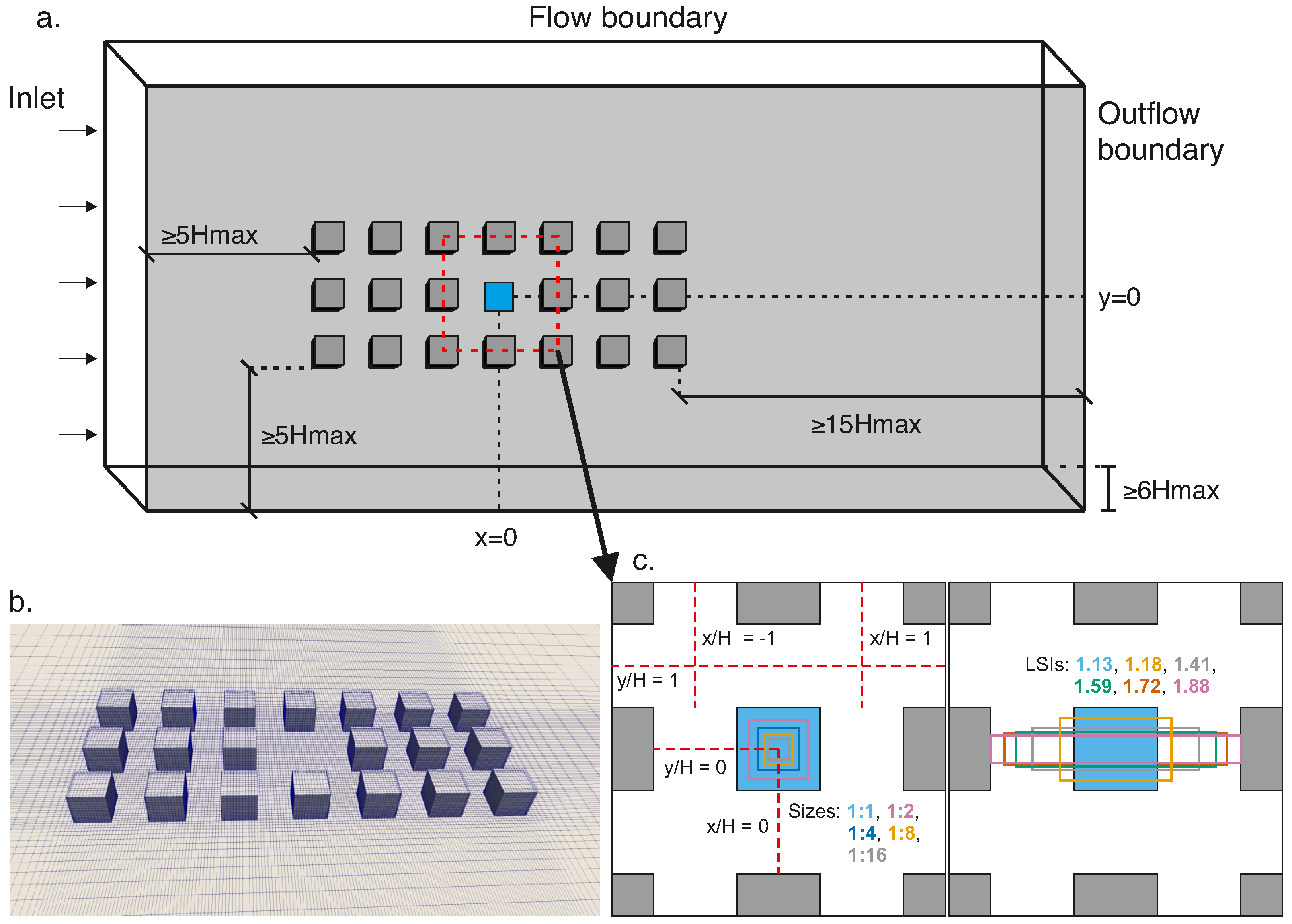
2.4.3. Computational Domain

Following the best practice guidelines for flows in an urban environment [39,40], the inlet is located at a distance $5H$ from the building array, the lateral boundaries are located at $7.5H$, the top boundary at $5H$, while the outlet is $15H$ away from the buildings so that a fully developed wake flow is achieved. The final dimensions of the computational domain are $33H\times 35H\times 6H$ in the streamwise, spanwise and vertical directions. Figure 1a sketches the domain geometry. This configuration ensures that the blockage ratio and the directional blockage ratio [41] are below $3\%$ and $17\%$, respectively.

The computational grid is a Cartesian, orthogonal and structured mesh consisting of $846,976$ cells. The grid is refined near the buildings to ensure a better spatial resolution in the region of interest (Figure 1b). Near the solid surfaces, the first computational cell is placed at a dimensionless wall distance of $y^{+}=y{u}_{\tau }/\nu >30$ (where y is the wall-normal direction and $u_{\tau }$ is the friction velocity). This required the use of wall functions for the accurate resolution of the wall-boundary layer [42]. Three meshes of different levels of refinement were analysed to ensure a mesh-independent solution. The Grid Convergence Index (GCI) [43,44] for the streamwise velocity and turbulent kinetic energy is 0.6% and 0.3%. The reader is referred to Ampatzidis et al. [22] for more details on the mesh independence study.

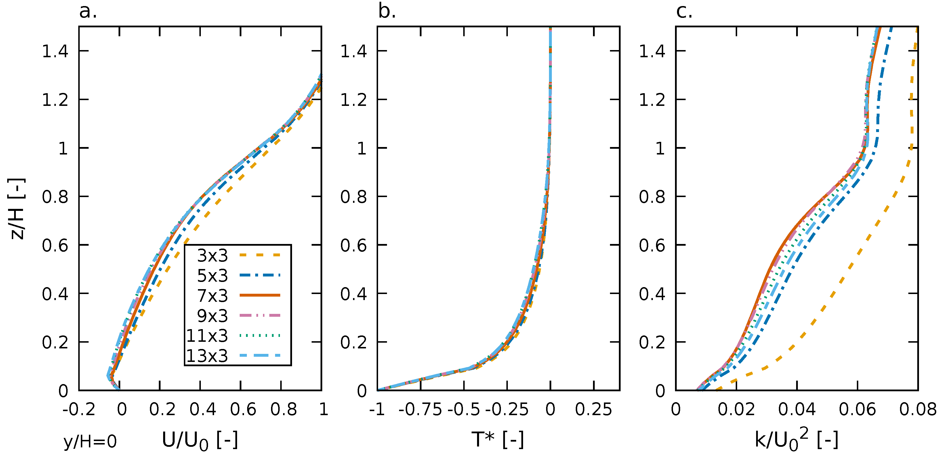
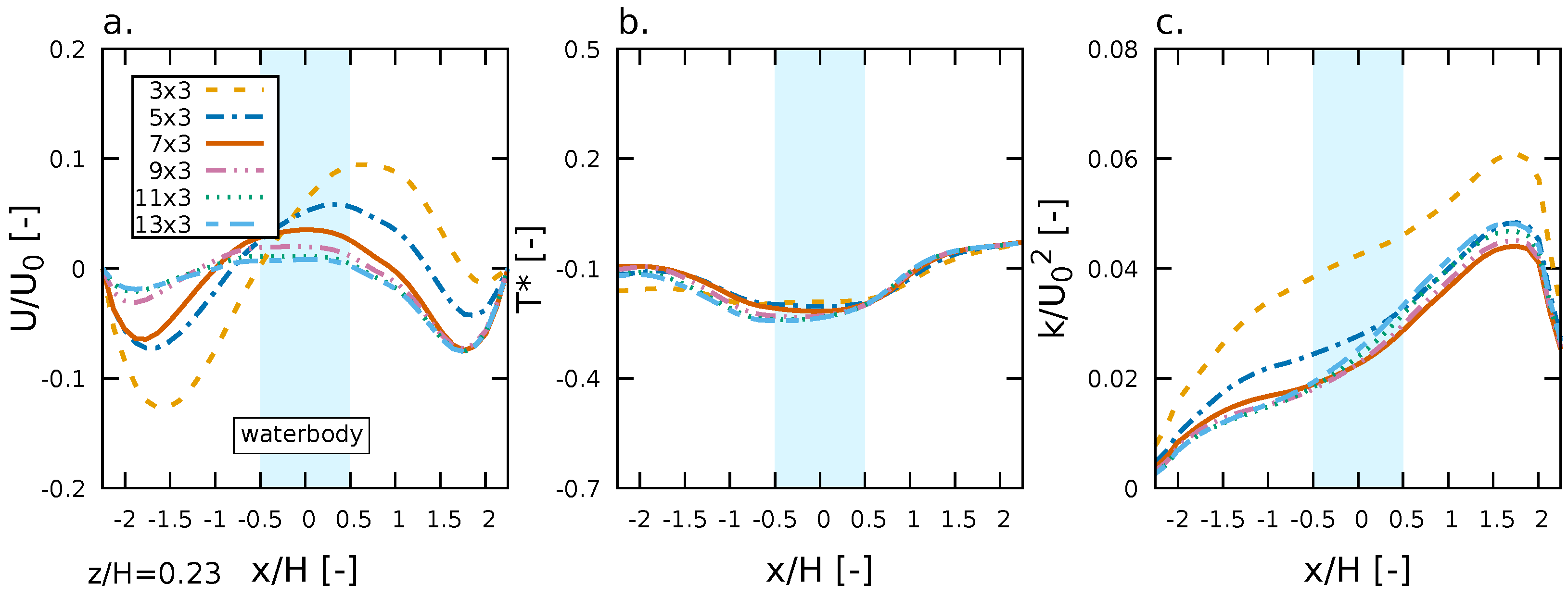
2.5. Sensitivity Analysis

The extent of the explicitly modelled built-up area is dependent on the influence the urban features have on the region of interest, in this case, the open square. According to Franke et al. [39], a minimum requirement of a building of height H should be represented if its distance from the region of interest is less than $6H$. Given that this study focuses on an idealised urban scenario, a sensitivity analysis is conducted to identify the necessary number of buildings needed. Initial simulations showed that there is minimal impact on the flow when more than three rows of buildings are employed. This is mainly because the approaching flow is parallel to the streamwise direction and the symmetry of the selected configuration. Therefore, the sensitivity analysis is carried out for three rows of buildings and six different numbers of buildings in the streamwise direction, namely a $3\times 3$, $5\times 3$, $7\times 3$, $9\times 3$, $11\times 3$ and $13\times 3$ building array. The simulations are conducted for both a warmer and a cooler water body leading to similar findings. Thus, results are only presented for the cooler water body for the sake of simplicity.

Figure 2 shows the vertical profiles of normalised streamwise velocity ($U/U_0$), temperature ($T^{*}=(T-T_a)/\Delta T_0$) and turbulent kinetic energy ($k/{U_0}^2$) in the middle of the open square and until a height of $z/H=1.5$ above the water body. For the streamwise velocity, only slight overestimation is observed closer to the water surface for the $3\times 3$ and $5\times 3$ arrays, while results for temperature are mostly identical. The main differences are observed for turbulent kinetic energy (TKE) where the results from the $3\times 3$ array clearly overestimated TKE values along the entire sampling line. For the $7\times 3$ array and beyond, TKE values seem to coincide with only minor discrepancies below roof level.

Figure 3 shows the horizontal profiles of normalised velocity, temperature and TKE in the middle of the open square and at pedestrian level ($z/H=0.23$). The simulated profiles present greater discrepancies compared to the vertical ones, especially in the region upwind of the water body. Again, the profiles tend to coincide as the building arrays become larger, with the $7\times 3$ standing out as a clear threshold for temperature and TKE. Notably, the $7\times 3$ array exhibits slight discrepancies for $U/U_0$ above the water body and larger ones in the upwind region. Nonetheless, an overestimation of the velocity of less than $U/U_0=0.05$ is considered acceptable, and hence the use of the $7\times 3$ array in this study is justified as a reasonable selection considering computational costs and loss of accuracy.

3. Results and Discussion

For each simulated scenario (see Table 1), the impact of the water body on the overall circulation in the urban neighbourhood is investigated by analysing the mean velocity field and the temperature and vapour concentration. Horizontal profiles and contours are extracted at pedestrian level ($z/H=0.23$), corresponding to 1.75 m at full scale [45,46]. The position of the sampling lines is depicted in Figure 1c. Turbulence effects are studied through the turbulent kinetic energy, and a focus on the exchange processes at the interface between buildings and the surrounding atmosphere is presented.

Three critical regions of interest are identified and used in the discussion that follows: (i) the open square, the area above and around the water body: $-1.5\le x/H\le 1.5$ and $0\le y/H\le 0.5$; (ii) downwind canyons (DC), the first and the second street canyon (in the spanwise direction) downwind from the water body; DC1: $2.5\le x/H\le 3.5$ and $0\le y/H\le 0.5$; DC2: $4.5\le x/H\le 5.5$ and $0\le y/H\le 0.5$; and (iii) the street canyon, with the axis in the streamwise direction, placed at the side of the open square: $-2.5\le x/H\le 6.5$ and $0.5\le y/H\le 1.5$.

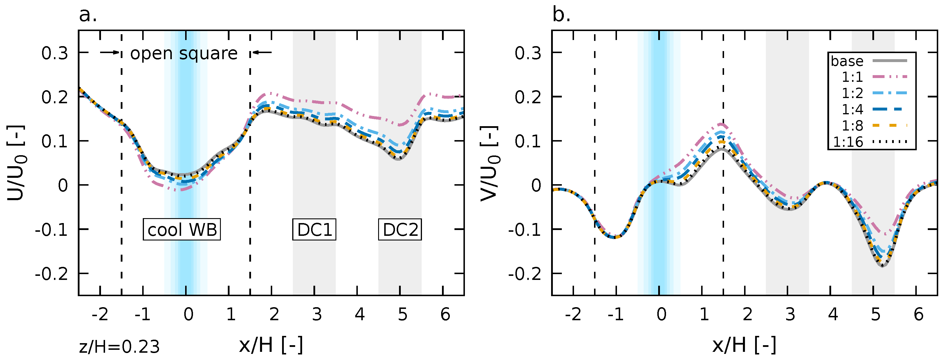
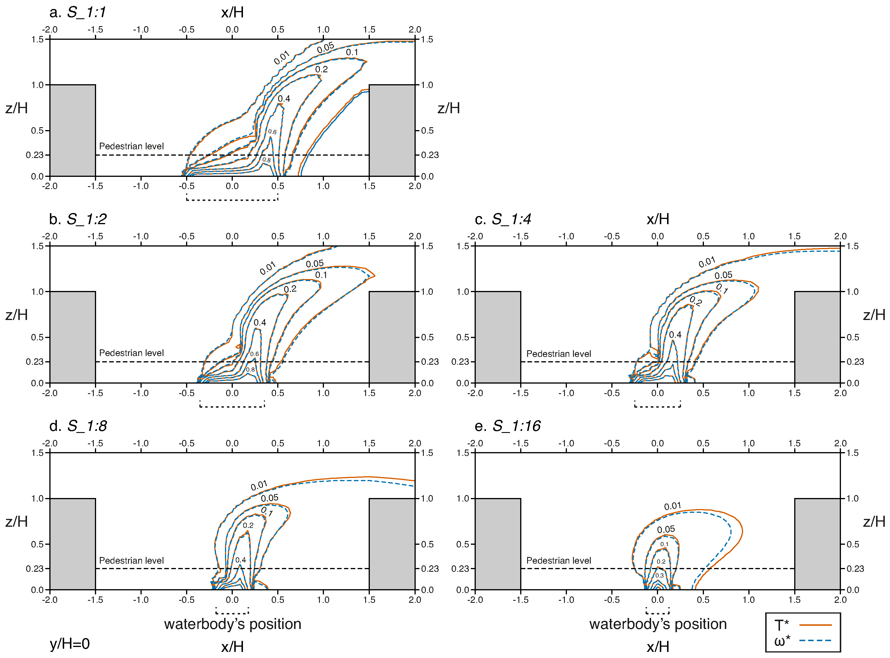
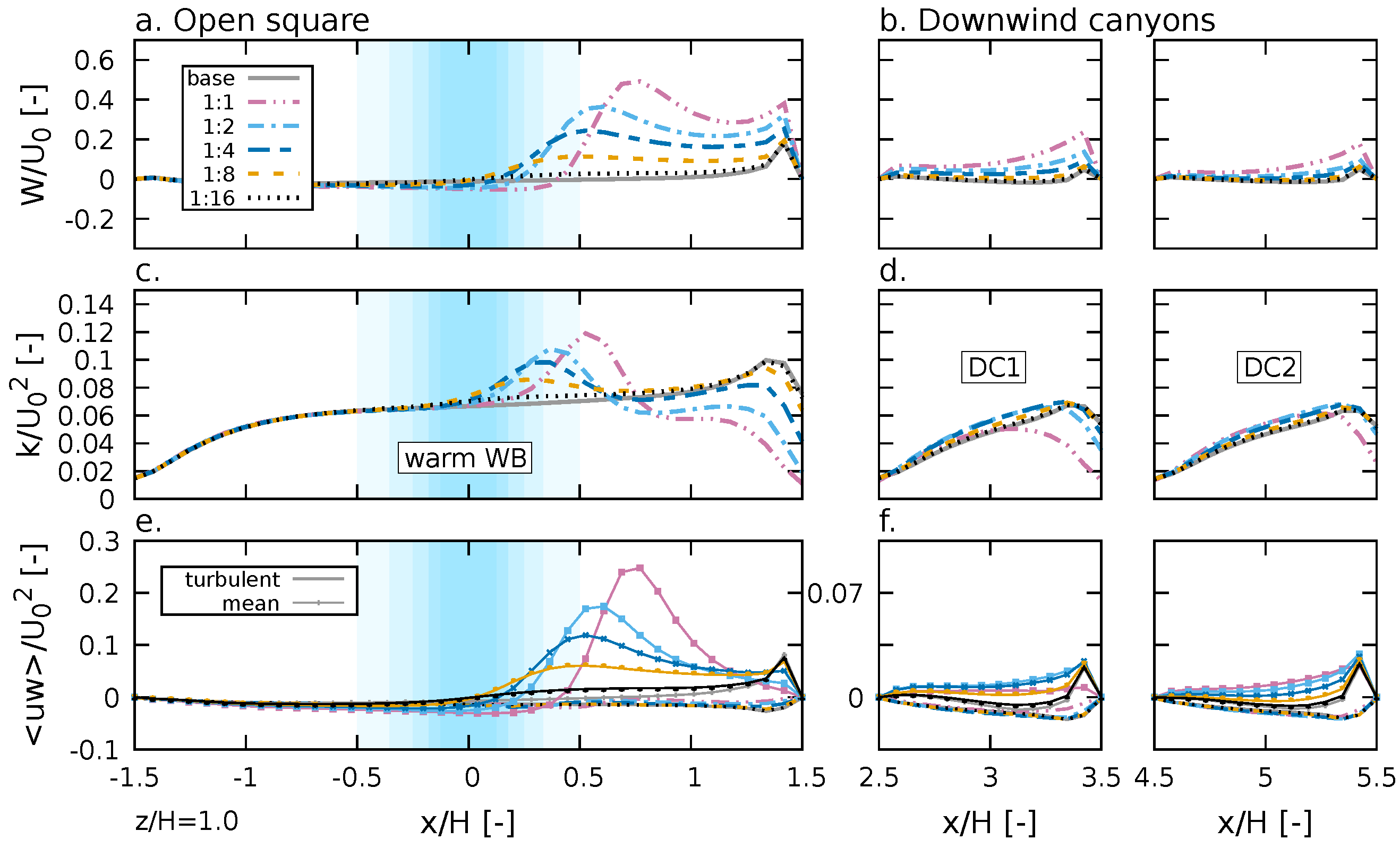
3.1. Varying Blue Space Size

In this section, results for the cases with different water body sizes are presented and discussed. The five different configurations are shown in Figure 1c. For the sake of simplicity, the cases with different water body sizes are referred to as S_1:1 (original), S_1:2, S_1:4, S_1:8 and S_1:16, as reported in Table 1.

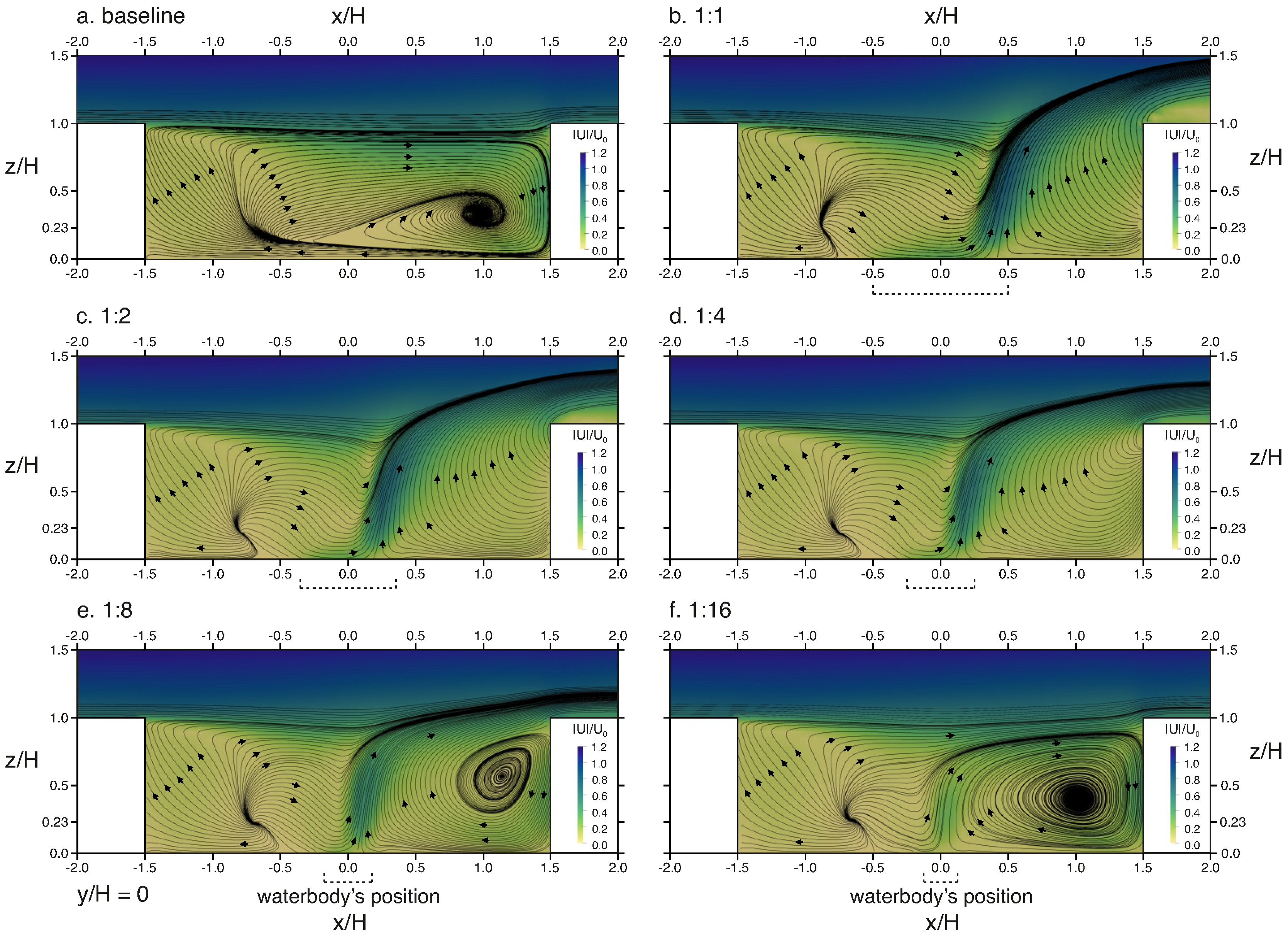
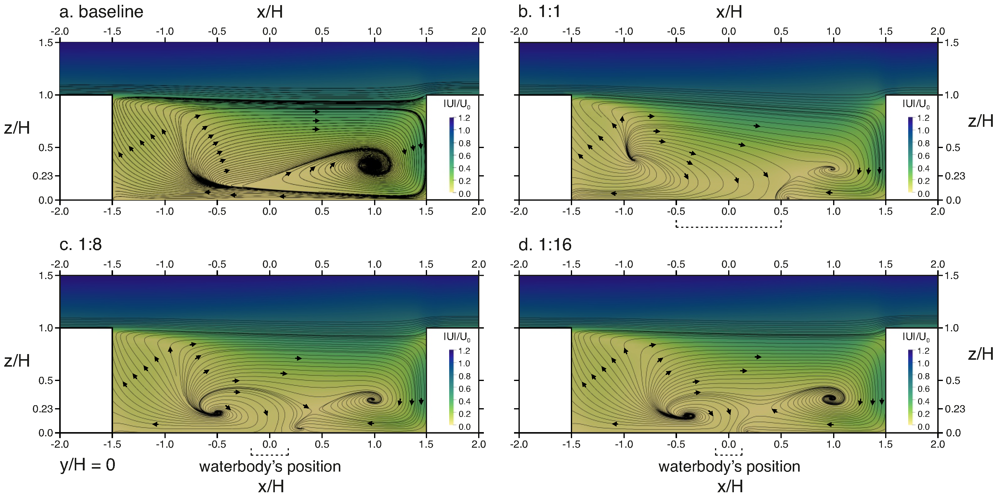
3.1.1. Mean Velocity Field

Figure 4 shows the non-dimensional velocity streamlines and the velocity magnitude for the case of a warmer water body over a vertical plane passing from the middle of the open square at $y/H=0$. Figure 4a displays the flow structure for the baseline scenario without the water body. The open square is dominated by a principal vortex induced by the atmospheric wind, which is a characteristic feature of an isolated roughness flow [47]. Near the ground ($0<z/H<0.1$), a reverse flow develops in the negative x direction, which is then deflected upwards, leading to an ascending flow that guides the air towards roof level ($z/H=1$). Figure 4b depicts the flow structure under the influence of the S_1:1 water body. What stands out in this figure is the strong upward buoyant flux that disrupts the flow structure of the baseline scenario in the above water body ($-0.5\le x/H\le 0.5$) and downwind water body ($0.5\le x/H\le 1.5$) areas, creating a vertical thermal plume that is advected by the main flow. In Figure 4c,d, results are shown for the cases with a S_1:2 and S_1:4 water body, respectively. It is apparent that the main features observed with the introduction of the S_1:1 water body remain, albeit with reduced magnitude. For instance, the weaker buoyant forces induced by the decreased size lead to a thermal plume that extends to lower heights: for the S_1:1 water body, the thermal plume extends approximately up to $z/H=1.5$, whereas for the S_1:2 and S_1:4 cases, the plume reaches $z/H=1.4$ and $z/H=1.3$, respectively. In Figure 4e, the size of the water body is further decreased to S_1:8. Interestingly, despite the presence of a weakened vertical motion that creates a thermal plume extending just above roof level ($z/H=1.23$), a clockwise-rotated vortex is created in the downwind water body area. The vortex extends in the range $0.8\le x/H\le 1.36$, with its centre located at $z/H=0.57$. These results suggest that under the presence of the S_1:8 water body, part of the induced vertical flux is not strong enough to escape beyond roof level and consequently enhances the primary vortex of the baseline scenario. When the water surface area is reduced to S_1:16 (Figure 4f), the buoyancy flux is entirely trapped below roof level, further enhancing the primary vortex, which is now extending in the range $0.1\le x/H\le 1.5$ and $0\le z/H\le 0.9$.

Figure 5 shows the impact warmer water bodies of different sizes have on the flow structure of the downwind canyons. Figure 5a depicts results for the baseline scenario, where it is apparent that both downwind canyons (DC1 and DC2) are dominated by a clockwise vortex, centred at the top-right corner, a characteristic feature of the skimming flow regime [48,49]. This vortex is generated and maintained as momentum is transferred downwards from the above-roof region [50], resulting in a clockwise flow within the canyon, separated from the flow above roof level ($z/H>1$). In Figure 5b, a potential pollutant removal mechanism is observed under the presence of the S_1:1 water body as the upward motion created in the open square is strong enough to disrupt the skimming flow regime in the downwind canyons. The clockwise vortex is destroyed, and the in-canyon flow is no longer separated from the atmospheric one. The results for the S_1:2 water body (Figure 5c) indicate that although the size of the water body is halved, the skimming flow in the downwind canyons is still disrupted; particularly in DC1, whilst in DC2, a small clockwise vortex persists. When the water surface area is further decreased to S_1:4 (Figure 5d), the flow structure in DC1 is partially disrupted, whereas there is no effect in DC2. Lastly, for the S_1:8 and S_1:16 cases (Figure 5e,f), the presence of a warmer water body has no effect on either downwind canyon.

In the case of a cooler water body under mixed convection, the size of the surface area has a minimal effect on the overall in-canyon flow structure. As an example, Figure 6 depicts velocity streamlines for the S_1:8 and S_1:16 water bodies, together with the baseline and S_1:1 water body scenarios. One notable difference is that the weaker downward motion caused by the cooler but smaller water bodies is not strong enough to redirect the flow downwards. Instead, velocity streamlines above the S_1:8 and S_1:16 water bodies remain parallel to the ground. In addition, the clockwise vortex at the bottom right of the open square is enhanced as the water body is reduced in size.

Figure 7 presents the dimensionless streamwise and vertical velocity profiles for the warmer water body within the open square and downwind canyons over the domain’s centreline ($y/H=0$) at pedestrian level. In the open square (Figure 7a), the streamwise velocity profiles for the baseline scenario present mostly negative values along the entire line, with near-zero positive values above the water body. For the warm water body cases, the upward vertical motion leads to increased positive values in the upwind and above-water body area, whilst higher negative values are present in the downwind part. The reduction of water body size diminishes wind speed changes in the above and upwind water body regions. In the downwind canyons (Figure 7c), the profiles of all cases mostly collapse to those of the baseline. Negative streamwise velocities are observed across the entire canyons, indicating a dominant reverse flow. Figure 7b depicts the profiles of vertical velocity in the open square. For the baseline scenario, increased negative values are observed near the downwind building’s facade per the direction of the principal vortex (see Figure 4a). With the S_1:2 and S_1:4 water bodies, the vertical velocities are positive, corroborating the disruption of the flow structure. However, under the presence of the smaller water bodies, the profiles tend to return to the baseline, particularly for the S_1:8 and S_1:16 cases. For the baseline, near-zero positive values are present in the rest of the open square, whilst similar to the streamwise velocity, the buoyancy forces induced by the presence of warmer water bodies lead to increased vertical velocities in the above and downwind water body area. The larger the water body, the higher the vertical velocity above the water body is. The profiles remain mostly unaffected in the upwind water body region. In the downwind canyons (Figure 7d), the clockwise vortex as seen in the baseline scenario (Figure 5a) leads to negative vertical velocities near the downwind building’s facade, whilst weak positive values are observed in the upwind part. The cases with a S_1:8 and S_1:16 water body collapse to the baseline profile (skimming flow persists), whereas as the size increases, the downward flow is considerably decreased to near-zero values, indicating the destruction of the skimming flow regime.

Figure 8 shows the normalised streamwise and spanwise velocity profiles over a horizontal line across the middle of the street canyon ($y/H=1$) at pedestrian level for the warm water body cases. In Figure 8a, the streamwise velocity profiles match in the upwind water body area as the influence of buoyancy is only felt along the direction of the prevailing wind. In the $0\le x/H\le 1.5$ region, streamwise velocities increase for all cases. Beyond the open square ($x/H>1.5$), further increased values are observed, with the exception of the S_1:16 case which collapses to the profile of the baseline scenario. Results in Figure 8b for the S_1:1 case suggest that the strong vertical plume leads to negative values of spanwise velocity both in the open square and downwind canyons, indicating increased channelling and hence better ventilation. As expected, values of spanwise velocities decrease with a decreasing water body size. For the S_1:16 case, the profile approximates the baseline, and there is no effect in the downwind canyons. The only scenario where the influence of a water body can reach DC2 is the S_1:1 one.

Figure 9 shows the normalised streamwise and spanwise velocities for the cool water body cases at $y/H=1$, i.e., the middle of the street canyon. What is apparent from the results is that the S_1:1 water body leads to near-zero streamwise velocities in the range $-0.5\le x/H\le 0.5$. This can be attributed to the strong downward motion induced by the cooler water surface which suppresses streamwise velocities over and around the water body. This increased downward motion is directed towards the downwind building and away from the water body, as shown in Figure 9b, leading to increased streamwise velocities beyond the open square and into the street canyon. This effect is less significant as the water body size decreases, and the profiles tend to return to the ones of the baseline scenario.

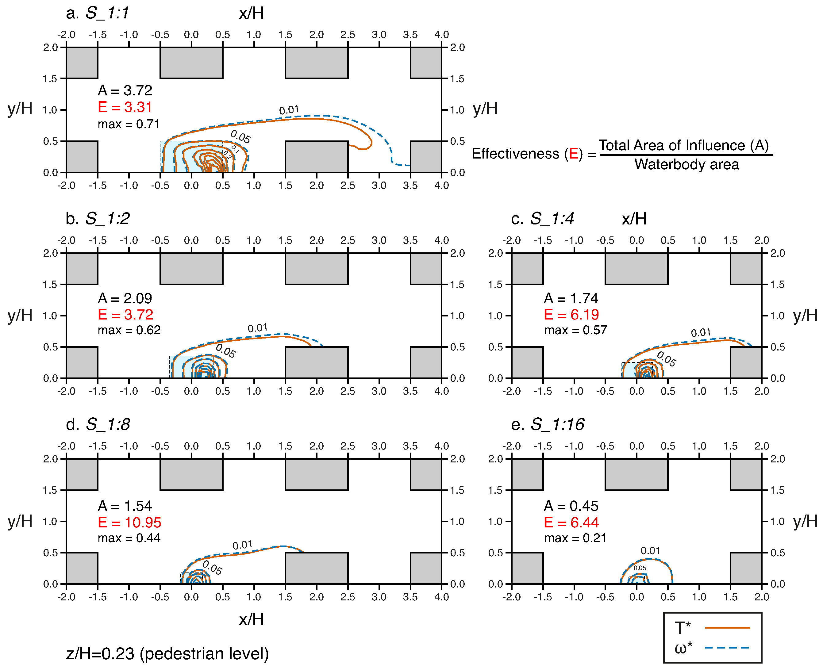
3.1.2. Temperature and Water Vapour Field

Temperature and vapour concentration are made non-dimensional utilising the building height H for length and the free stream velocity $U_0$ for velocity. Temperature is normalised as $T^{*}=(T-T_a)/\Delta T_0$ and vapour concentration as ${\omega }^{*}=(\omega -{\omega }_a)/\Delta {\omega }_0$. Since the model assumes heat and mass analogy, the profiles of $T^{*}$ and ${\omega }^{*}$ are primarily similar. Hence, for the sake of simplicity, the discussion in this section is focused on $T^{*}$, and equal consideration is implied for ${\omega }^{*}$. The results represent changes in temperature and water vapour against the baseline scenario without the water body. Absolute values in the cool water body cases indicate a decrease in temperature and an increase in water vapour.

Figure 10 depicts contours of $T^{*}$ and ${\omega }^{*}$ over a vertical plane in the streamwise direction in the middle of the open square for the case with a warmer water body and different sizes. What is apparent is that a thermal plume extending above roof level in the streamwise direction can only be observed for the S_1:1, S_1:2 and S_1:4 cases. For the 1:8 case, only a minimum effect is present above roof level, i.e., the 0.01 contour line, which is not strong enough to create a thermal plume and, thus, re-attaches at the downwind building. When the S_1:16 is introduced, the induced temperature/vapour gradient near the water surface does not generate enough upward buoyancy capable of directing the flow beyond roof level. This observation signifies severe implications for thermal comfort, as the accumulation of water vapour at pedestrian level can exacerbate heat stress. As an example, a ${\omega }^{*}=0.2$ increase means that, locally, relative humidity increases from 60% to about 70%. Overall, the profiles match the streamlines in Figure 4, and the upwind water body area remains unaffected by the evaporation process.

Figure 11 shows the contours of normalised temperature ($T^{*}$) and water vapour (${\omega }^{*}$) over a horizontal plane at pedestrian level for the cases with a warmer water body and different sizes. The lateral effects are mostly constrained within the open square with large temperature/water vapour gradients around the water surface due to the strong upward motion which dominates the flow. However, as the water body decreases in size and more warmer air and water vapour remain below roof level (as shown in Figure 10), the effectiveness of the water body increases. We define this effectiveness (E) as the ratio between the total area of influence up to which blue space effects are felt, i.e., $T^{*}={\omega }^{*}=0.01$ and the area of the water body. As shown in Figure 11a–d, blue space effectiveness more than triples from $E=3.31$ for the S_1:1 to $E=10.95$ for the S_1:8 case. The largest increase in E is observed between the S_1:4 and S_1:8 cases (from $E=6.19$ to $E=10.95$, respectively), which can be explained by looking at Figure 4e where it is shown that for the S_1:8 case, a recirculating vortex is created, indicating that significantly more air is trapped below roof level. The influence of size in decreasing effectiveness is depicted in Figure 11e, where the S_1:16 water body has $E=6.44$, indicating that since there is no escaping flow in the vertical direction, the smaller size leads to less lateral spread.

Figure 12 shows the $T^{*}$ and ${\omega }^{*}$ contours over a horizontal plane at pedestrian level for the cases with a cooler water body and different sizes. Compared to the cases with a warmer water body, the magnitude of the influencing area and effectiveness increases as there is no upward flow that breaks beyond roof level, and thus, the effects are more spread in both the lateral and streamwise directions. As expected, the larger the water body, the larger the influencing area. Nonetheless, the relationship between size and E is not linear, as the results suggest that the S_1:4 water body presents the highest cooling effectiveness ($E=32.75$) and the S_1:16 one the lowest ($E=13.51$). This counter-intuitive finding, whereby the largest water body is not the most effective, can be explained by looking at the velocity profiles in the street canyon ($0.5\le y/H\le 1.5$) for all cases in Figure 9. The S_1:1 case presents the lowest streamwise velocities in the street canyon, indicating the existence of a vortex that hinders the advection of temperature and water vapour further downwind, thus limiting the cooling effectiveness. As the water surface area decreases, the recirculating vortex decreases in size, streamwise velocities increase and more air that is drawn towards the water body can escape the open square and be directed downstream, leading to a slight increase of the cooling effectiveness. This is the case for the S_1:2 and S_1:4 cases. For the S_1:8 and S_1:16 cases, the velocity profiles in the street canyon mostly match the one of the baseline scenario. However, size has become now the dominant influencing factor as the water bodies cannot harness the higher advection potential, and their cooling effectiveness drops.

3.1.3. Interface Flux Budget

The interface flux budget, i.e., the mass exchange between the urban canyons and the surrounding atmospheric flow is appraised by analysing the vertical kinematic fluxes at roof level using the following:

$$\langle uw\rangle =UW+\langle u^{\prime }{w}^{\prime }\rangle ,$$

(12)

where capital letters indicate mean quantities. The turbulent contribution to the fluxes is estimated using the $k-\epsilon$ turbulent model to express $\langle u^{\prime }{w}^{\prime }\rangle =-{\nu }_t(\partial U/\partial z+\partial W/\partial x)$, where ${\nu }_t$ is the turbulent kinematic viscosity [m${}^2$s${}^{-1}$]. Both the mean and turbulent terms are computed and reported separately.

Figure 13 shows the non-dimensional profiles of vertical velocity, TKE and flux budget over a horizontal line at roof level across the domain’s centre line for the cases with a warmer water body and different sizes. The profiles for the cases with a cooler water body show minimal discrepancies with respect to the baseline scenario and thus are not shown for simplicity. In the open square (Figure 13a), the S_1:1 water body demonstrates the highest values of $W/U_0$ in the downwind water body area, whilst as the water body decreases in size, the $W/U_0$ profile tends to return to that of the baseline scenario, i.e., without the water body. This increase in vertical velocities is also observed in the downwind canyons (Figure 13b). In Figure 13c, the TKE profiles of all cases exhibit a peak in the above-water body area and decreased values near the downwind building’s edge. Again, the smaller the water body is, the more its TKE profile tends to collapse to the baseline one. In the downwind canyons (Figure 13d), high values of TKE are observed near the downwind building’s edge for all cases, except for the square water body, where the strong thermal plume has decreased the shear at roof level leading to decreased TKE values. In Figure 13e,f, the vertical momentum fluxes for all cases are presented. In the open square (Figure 13e), a significant increase of mean vertical fluxes is observed for the larger water bodies right downstream of the water surface due to the strong vertical motion, indicating intense vertical exchange. In contrast, the turbulent counterparts for all sizes show near-zero values across the entire length of the open square. In the downwind canyons (Figure 13f), the S_1:2 and S_1:4 cases exhibit the strongest momentum fluxes in DC1, whilst the S_1:1 water body presents higher values in DC2.

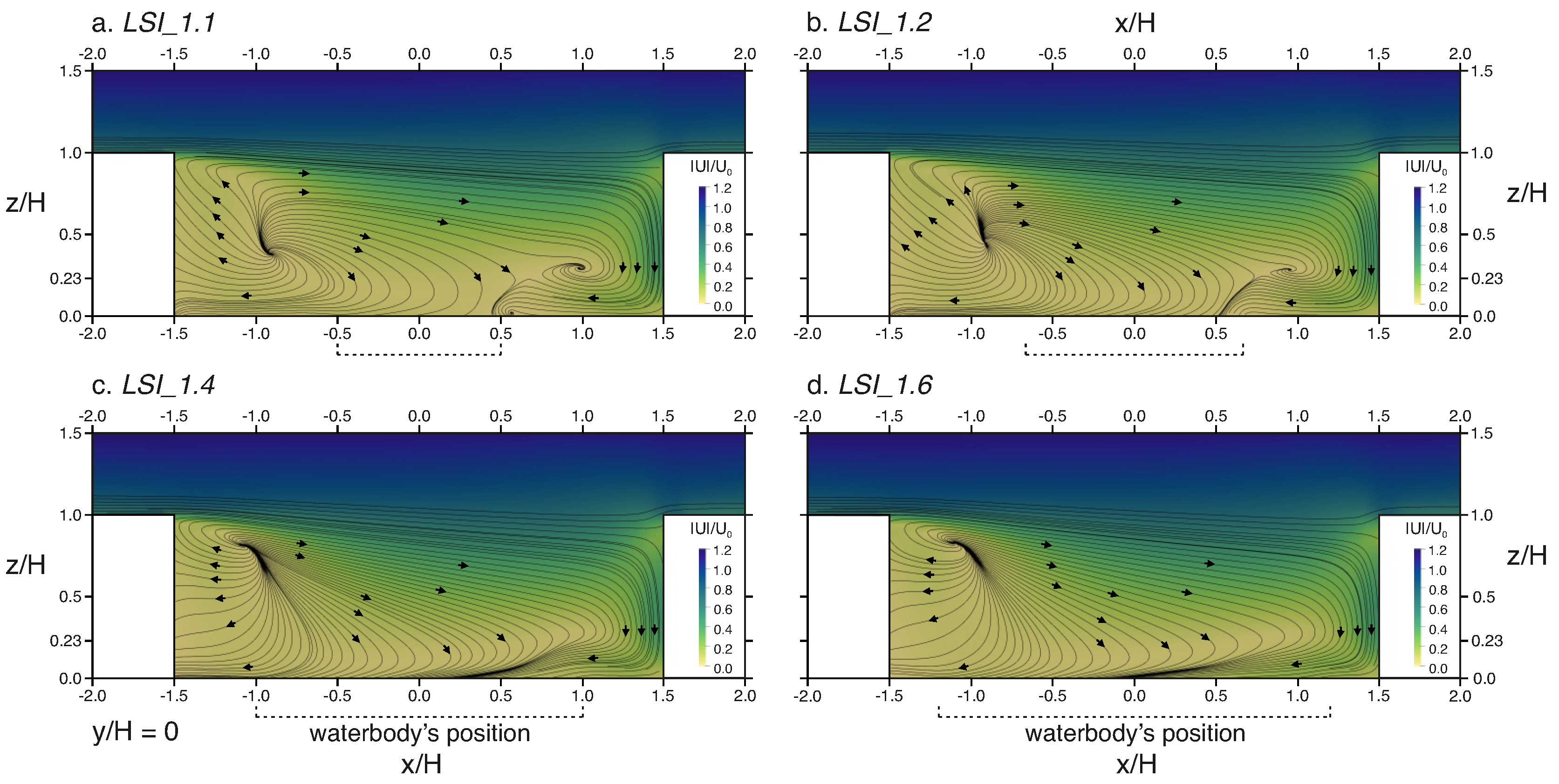
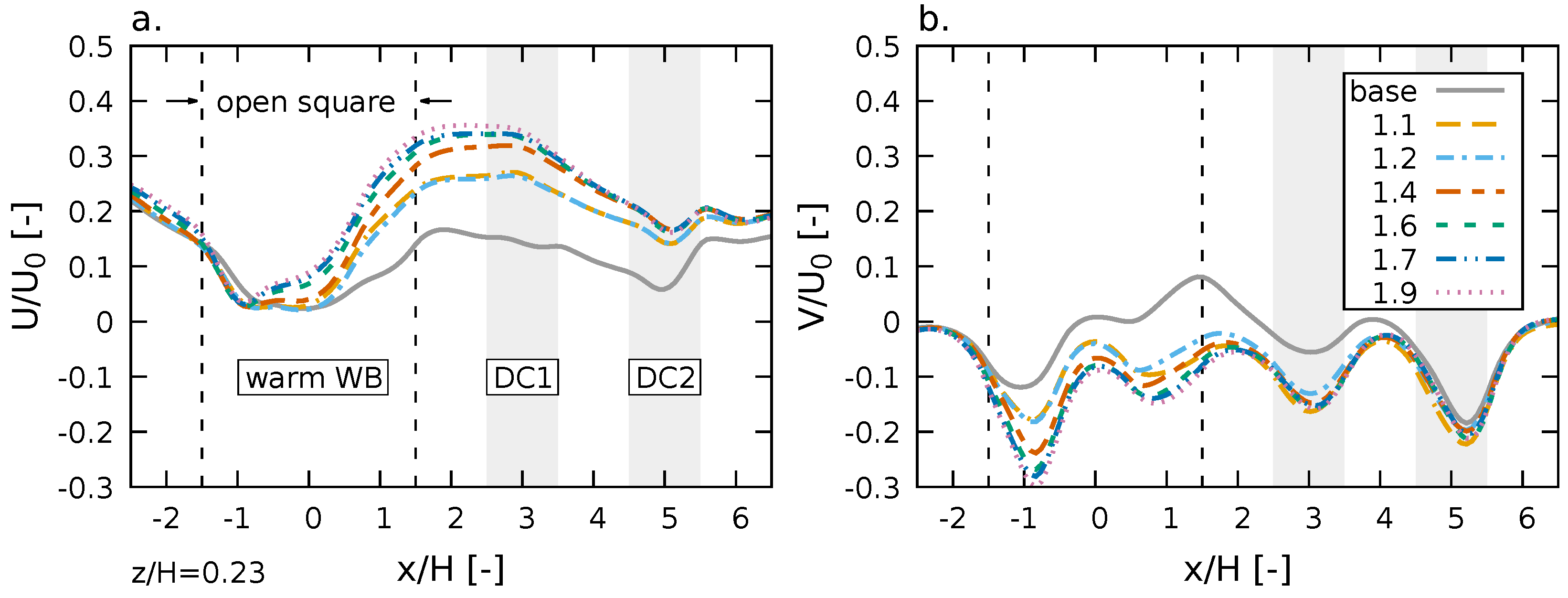
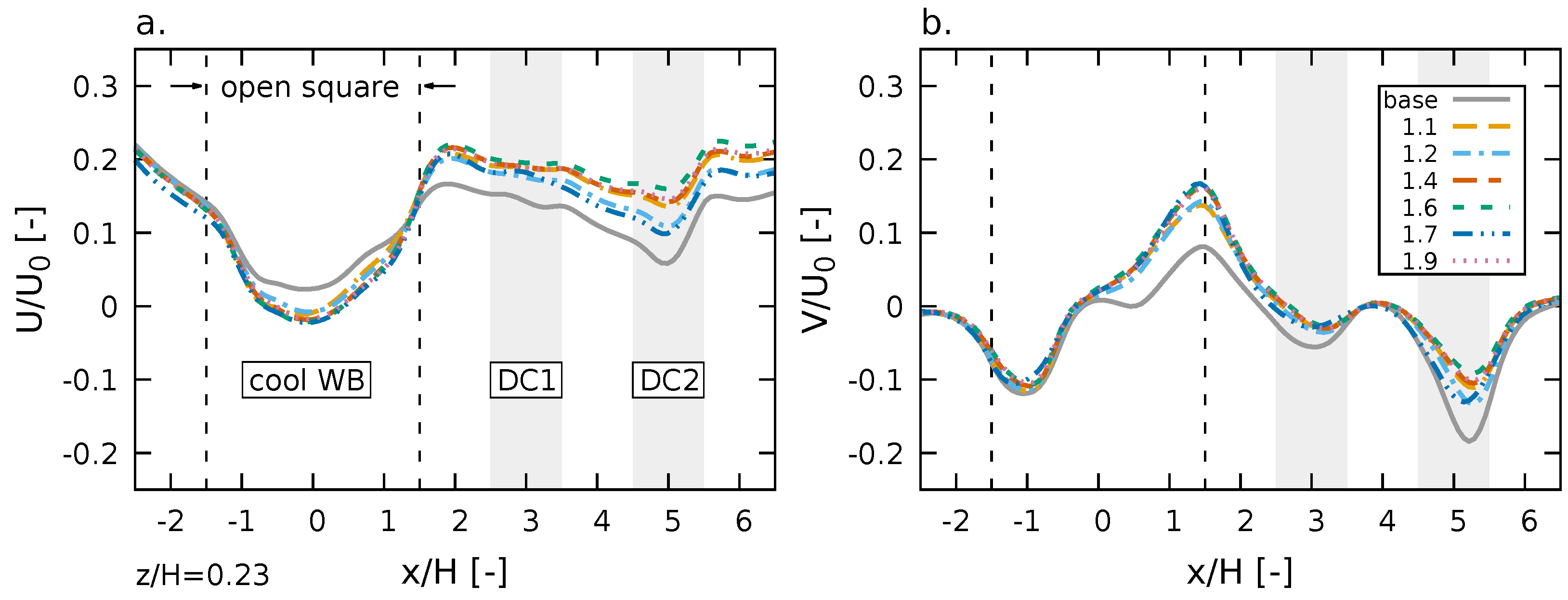
3.2. Varying Blue Space Shape

In this section, results for the cases with different shapes are presented and discussed. The six different configurations are shown in Figure 1c. For the sake of simplicity, the cases with different $LSI$ values are referred to as LSI_1.1 (original), LSI_1.2, LSI_1.4, LSI_1.6, LSI_1.7 and LSI_1.9, as reported in Table 1.

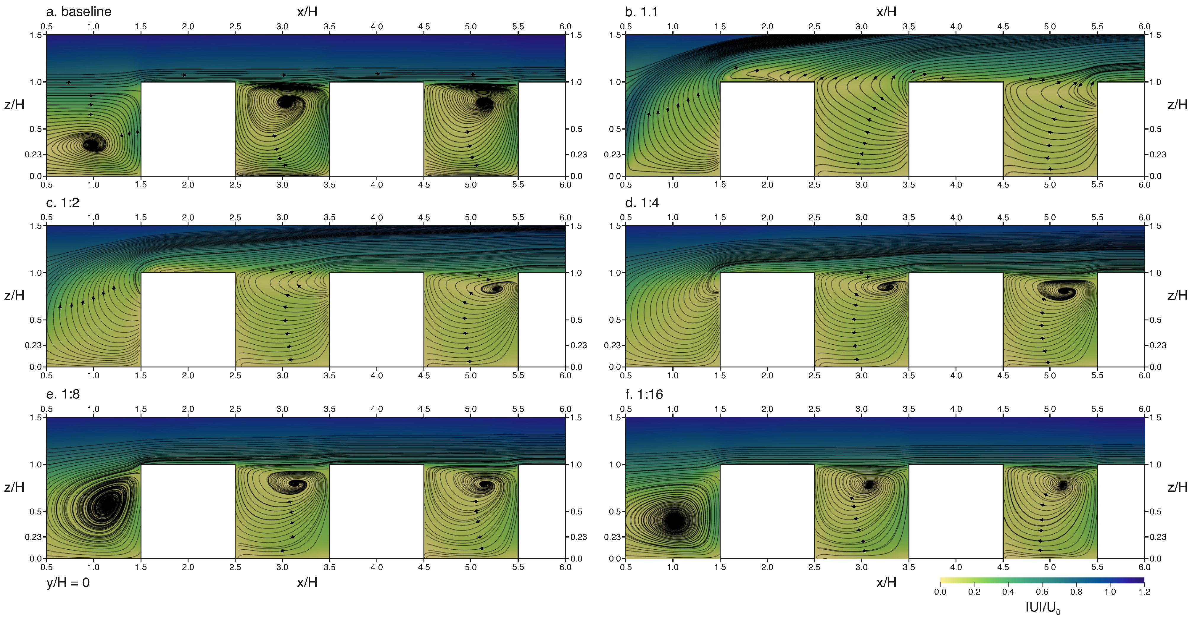
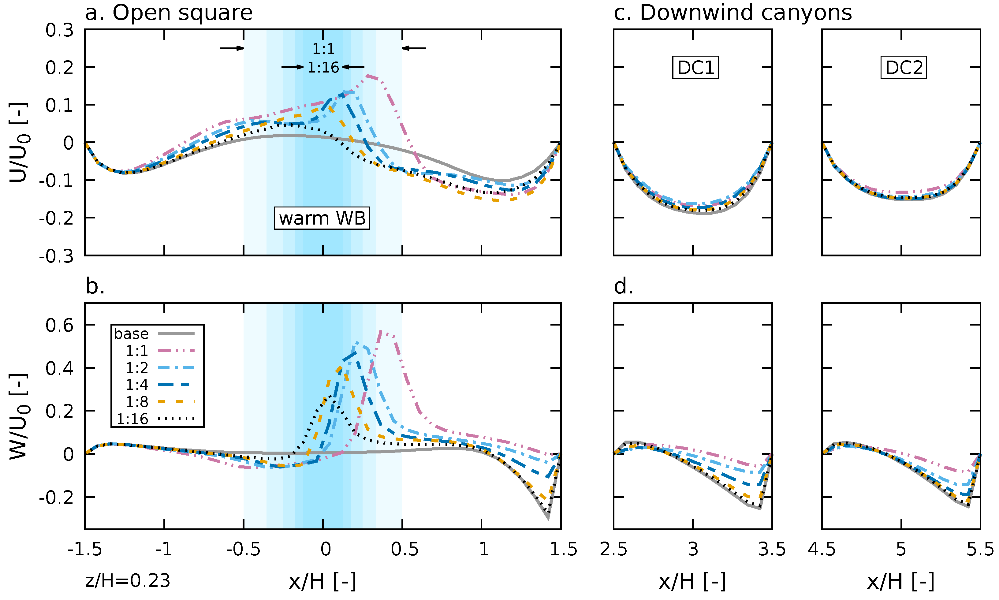
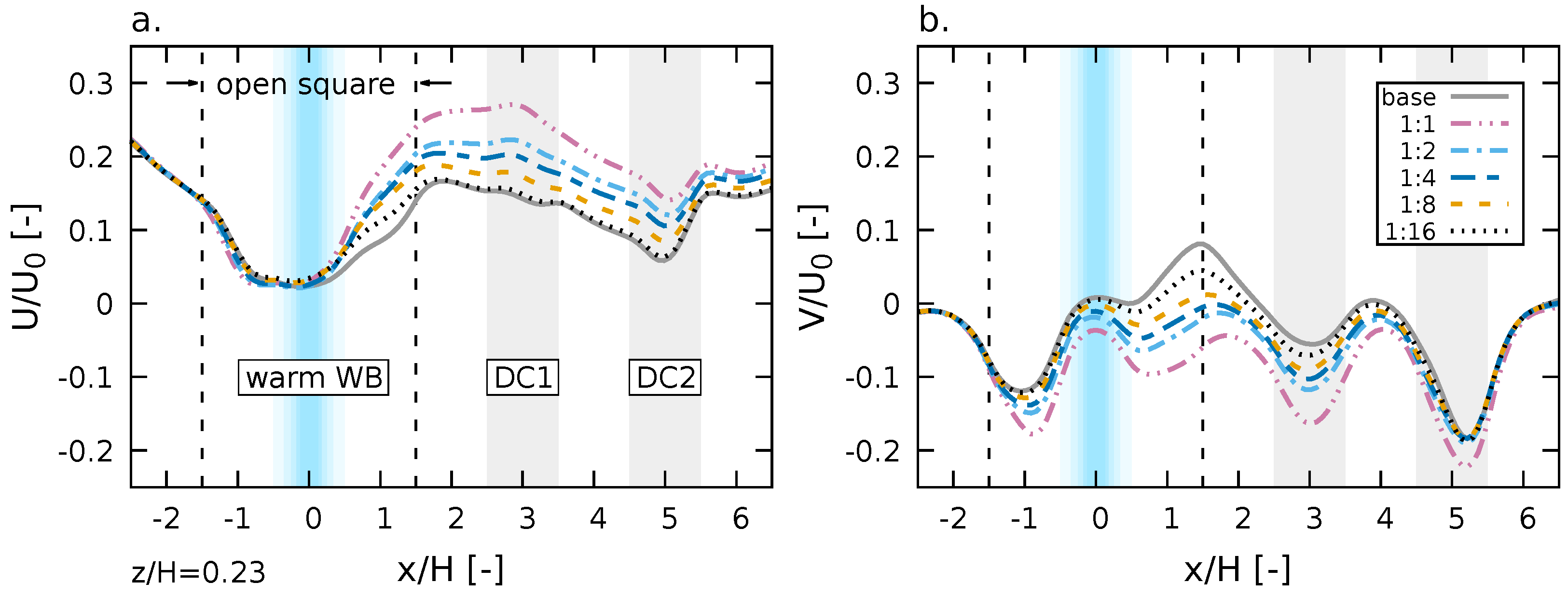
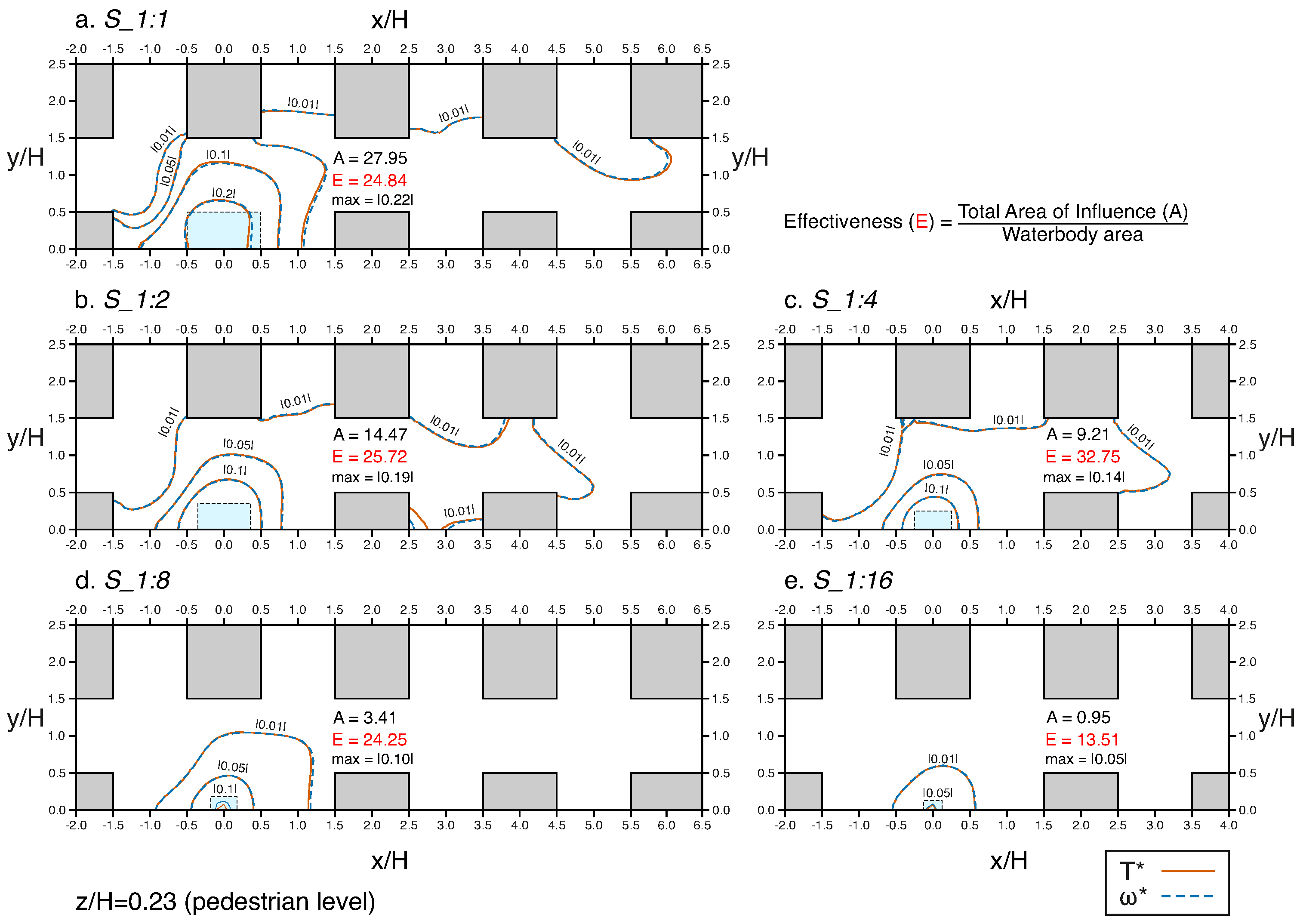
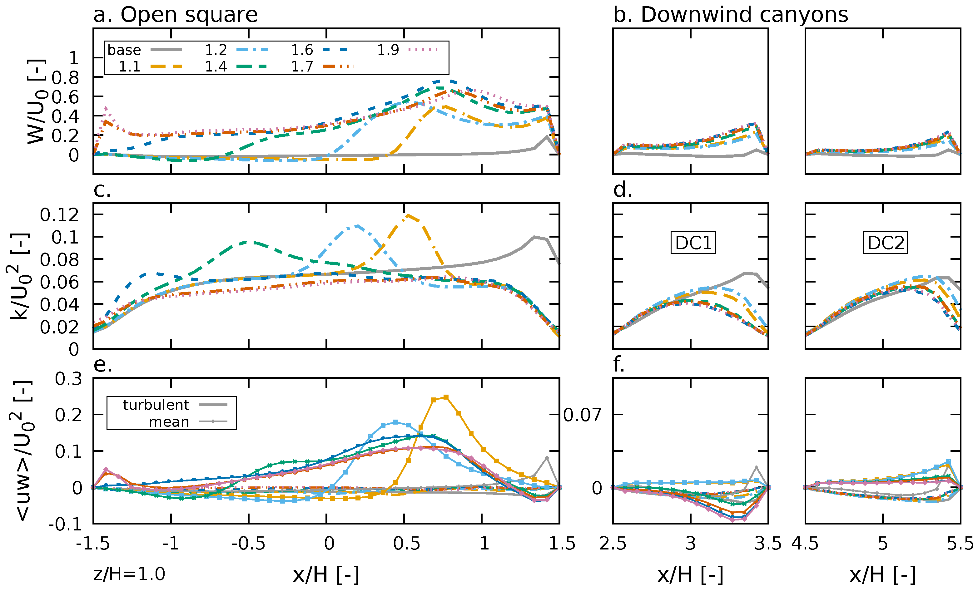
3.2.1. Mean Velocity Field

For the cases with a warmer water body, the flow structure is dominated by the upward buoyant flow that extends beyond roof level, similar to the original LSI_1.1 case (Figure 4b). The only difference in the flow structure over a vertical section at the middle of the open square ($y/H=0$) is that the wider the water body becomes, the larger the area the buoyant flux occupies within the open square. For instance, the LSI_1.9 case, where the water body occupies the entire length of the open square, leads to an upward vertical motion across the entire section.

Figure 14 shows the velocity streamlines and velocity magnitude for the cases with a cooler water body and different shapes. Results are shown only for the original LSI_1.1 water body and three additional shapes, namely LSI_1.2, LSI_1.4 and LSI_1.6, as no significant changes were observed for higher $LSI$ values. Contrary to the cases with a warmer water body, the variation in shape with a cooler water body alters the flow structure. As the water body becomes lengthier and narrower, the vortex at the bottom right of the open square becomes weaker and eventually disappears for the LSI_1.4 case. A further change in shape does not drastically alter the overall flow structure within the open square. In the downwind canyons, regardless of the shape, the disruption of the skimming flow persists (see Figure 5b) for the warm water body cases, whilst there is no alteration for the cool water body cases.

Figure 15 shows normalised streamwise and vertical velocity profiles in the middle of the open square and within the downwind canyons at pedestrian level for the warm water body cases and different shapes. The results suggest that higher $LSI$ values lead to increased streamwise velocities both within the open square and the downwind canyons (Figure 15a,c). More specifically, the LSI_1.2 case presents the highest streamwise velocity of about $U/U_0=0.25$ in the middle of the open square, whilst the LSI_1.7 and LSI_1.9 cases observe a large peak in negative values ($U/U_0\approx 0.2$) in the upwind and downwind water body areas. As expected, results in Figure 15b depict increased vertical velocities along the open square section as the $LSI$ values become higher. However, due to the fact that the larger the $LSI$, the narrower the water body and, thus, the smaller the fetch in the spanwise direction, peak vertical velocities are lower for the cases with a large $LSI$. The values of $W/U_0$ in the downwind canyons remain mostly unchanged (Figure 15d). The variation in shape for a cooler water body has minimal effect on $U/U_0$ and $W/U_0$ values in the open square and downwind canyons; thus, the results are not shown.

Figure 16 shows normalised streamwise and spanwise velocity profiles in the middle of the street canyon ($y/H=1$) at pedestrian level. In Figure 16a, and similar to what has been discussed for the original LSI_1.1 case in Figure 8, increased $U/U_0$ values are observed beyond approximately the middle of the open square at $x/H=0$. Nonetheless, it has been shown that the higher the $LSI$, the higher the streamwise velocity, e.g., for the LSI_1.9 case, values of about $U/U_0=0.35$ are observed downwind from the open square in the range $1.5\le x/H\le 2.5$. This feature can be explained by the fact that as the $LSI$ increases, the open space between the water body and the downwind building decreases. This means that the air drawn into the open square by the upward flow is squeezed into a smaller area as it is directed towards the street canyon and is thus accelerating. An analogous situation is true for the spanwise velocities within the open square, where the largest values are observed for the higher $LSI$ cases. The discrepancies become less prominent downwind from the open square.

For the cases with a cooler water body (Figure 17), the profiles of $U/U_0$ and $W/U_0$ mostly match the ones shown for the original LSI_1.1 case in Figure 9. Downwind from the open square, where the original case showed increased streamwise velocities, the LSI_1.6 case presents slightly higher values, whilst decreased $U/U_0$ values are observed for the LSI_1.2 and LSI_1.7 cases. Results for spanwise velocities present fewer discrepancies.

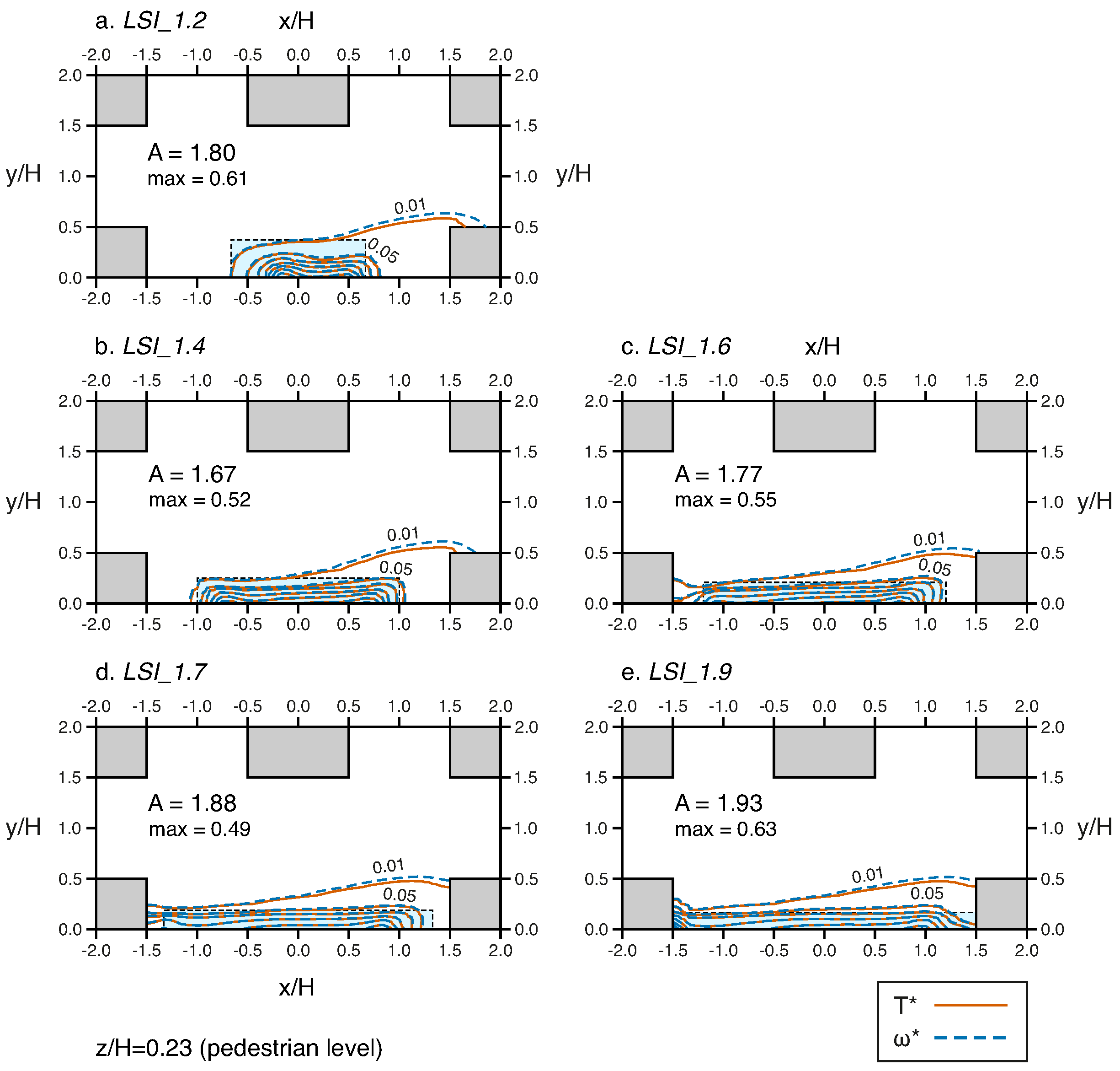
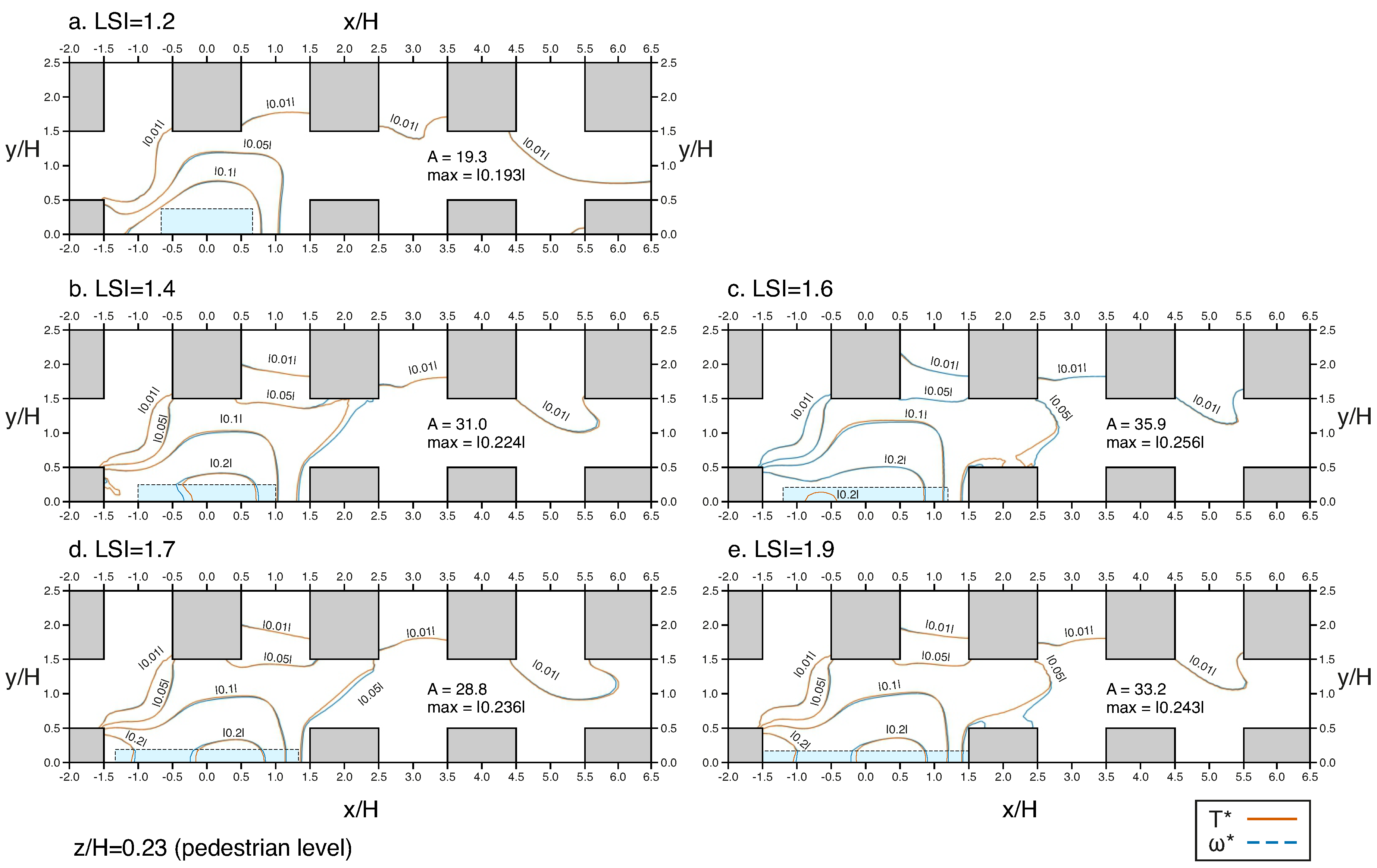
3.2.2. Temperature and Water Vapour Field

For the cases with different shapes, contours of temperature and water vapour over a vertical section in the middle of the open square share qualitatively similar profiles with the original LSI_1.1 case (e.g., Figure 10a). For the warm water body cases, the upward buoyant fluxes extend temperature and water vapour effects beyond roof level. The higher the $LSI$ is, the less intense the effects at a specific height, but they are more spread along the streamwise direction.

Figure 18 depicts contours of $T^{*}$ and ${\omega }^{*}$ over a horizontal plane at pedestrian level for the cases with a warmer water body and different shapes. The reader is referred to Figure 11a for the results of the original LSI_1.1 case. As the size of the water body is kept constant, the effectiveness is measured by simply comparing the total area within which blue space effects are felt. The original LSI_1.1 case of a square water body is the most effective, covering an area of 3.72 m${}^2$. The second most effective shape is the LSI_1.9 one, whose effects cover an area of 1.93 m${}^2$ (Figure 18e). This can be attributed to the fact that the lengthier a water body is, the larger its perimeter, leading to increased heat exchange with its urban surroundings [19]. This is the case for the LSI_1.4, LSI_1.6, LSI_1.7 and LSI_1.9 cases where the warming effectiveness gradually increases. Nonetheless, it is apparent that the LSI_1.2 case, as well as the original LSI_1.1, are wide enough that their effects reach the street canyon and are thus advected downwind, leading to increased effectiveness.

Figure 19 depicts contours of $T^{*}$ and ${\omega }^{*}$ over a horizontal plane at pedestrian level for the cases with a cooler water body and different shapes. The reader is referred to Figure 12a for the results of the original LSI_1.1 case. Similar to what has been discussed in Figure 12, temperature and water vapour effects under the presence of a cooler water body are spread across a larger area. What is striking about the results in Figure 19 is that out of the six configurations, including the original square water body (LSI_1.1), the most effective shape is the LSI_1.6, followed by the LSI_1.9. Despite the near-zero values of streamwise velocity in the open square for all cases (Figure 17a), the LSI_1.6 case presents higher values in the street canyon further downwind, meaning that scalars can be transported more effectively.

3.2.3. Interface Flux Budget

Figure 20 shows normalised profiles of vertical velocity, TKE and flux budget over a horizontal line at roof level across the domain’s centre line for the cases with a warmer water body and different shapes. The profiles for the cases with a cooler water body show minimal discrepancies and are not shown. In the open square (Figure 20a), and contrary to the situation at pedestrian level (Figure 15b), the original LSI_1.1 water body leads to the lowest vertical velocities at roof level. This can be attributed to the fact that along this specific sampling line, i.e., at $y/H=0$, more air is experiencing an upward motion enhancing the vertical velocities as it is directed downstream. The highest peak in $W/U_0$ at roof level is observed for the LSI_1.6 case in the downwind water body area, indicating that there does not exist a linear relationship between $W/U_0$ and $LSI$, as appeared to be the case at pedestrian level (Figure 15b). In the downwind canyons (Figure 20b), all cases present similar profiles, except with slightly decreased vertical velocities for the LSI_1.1 and LSI_1.2 cases.

In Figure 20c, the TKE profiles of all cases exhibit decreasing magnitude as the $LSI$ becomes bigger. In addition, the higher the $LSI$, the more upwind the peak in TKE is observed. In the downwind canyons (Figure 20d, the strong thermal plume reduces the shear leading to decreased TKE values, with the LSI_1.4, LSI_1.6, LSI_1.7 and LSI_1.9 exhibiting similar and further reduced values. In Figure 20e,f, the vertical momentum fluxes for all cases is presented. In the open square (Figure 20e), every variation in shape leads to a decreased vertical exchange compared to the original square water body. The peaks are mostly observed above and downwind from the water body area. In the downwind canyon DC1 (Figure 20f), the LSI_1.1 and LSI_1.2 cases exhibit weak positive mean values, whereas higher negative values are observed for the rest of the cases. This is an indication that the streamwise velocity for the LSI_1.4, LSI_1.6, LSI_1.7 and LSI_1.9 cases at roof level is negative, meaning that under the presence of lengthier water bodies, the flow is drawn upwards and towards the negative x-direction before it is re-directed towards the streamwise direction beyond roof level. In DC2, the mean vertical component is positive regardless of the shape, albeit with decreasing magnitude as the $LSI$ becomes higher. The turbulent components exhibit weak negative values for all cases.

3.3. Limitations and Recommendations for Future Work

A limitation of this study is the assumption of neutral atmospheric conditions, which can be representative of a nighttime situation but not typical of other instances during the day [51]. Future research is needed to examine the impact of atmospheric stability on blue space effects at different parts of the day. Radiation and the resulting varying surface temperatures of buildings, ground and water surfaces were also ignored. Therefore, the influence of the in-canyon surface temperature differences on the thermal interaction between blue spaces and their urban surroundings would be a fruitful area for further work. In addition, transient simulations will be beneficial for future work to better understand the dynamics of the system as this study only examines steady-state conditions. Finally, the reproduction of the internal dynamics of the water body and the heat exchange between water and air can be considered important advancements as they will help to better assess the heating and cooling mechanisms induced by water. Nonetheless, this would require the modification of the numerical approach and would increase the level of complexity of the models, a not-so-straightforward task.

4. Conclusions

This research examines the influence of size and shape on the UHI mitigation potential of an isothermal blue space in an idealised urban neighbourhood, using a numerical solver described in Ampatzidis et al. [22]. The parametrisation of size and shape has been conducted in such a way so that the water body remains always obstructed by the prevailing wind in order to minimise its effects in assisting downwind advection.

The simulations have been set up to approximate a range of possible situations over a diurnal cycle or across different seasons whereby a water body warms/cools at a different rate than the land surface and ambient air, creating a temperature difference. Results suggest that during late-summer nights when water is warmer than the surrounding air, inadequately sized water bodies promote overturning and increased temperature and humidity levels at pedestrian level, thereby worsening environmental conditions and increasing the risk of heat-related illness and mortality. Additionally, small water bodies—in our case smaller than a quarter of the original square $1.5\times 1.5$ water body—do not induce a thermal plume strong enough to disrupt the skimming flow regime of downwind canyons. This favourable feature of warm water bodies is only present under the influence of the original square water body (S_1:1) and the S_1:2 and S_1:4 ones.

This study has also shown that despite the fact that larger water bodies influence larger areas and lead to greater temperature and humidity changes, their effectiveness, i.e., the ratio between the total area within which their effects are felt and their size, is dependent on the local velocity field. For instance, we have shown that if the square water body is reduced in size by a quarter, its effectiveness increases by about 30%. This can have important implications in the design and implementation of blue spaces for areas with limited open space. The results imply a potential change in the use of water bodies of different sizes. Larger water bodies, which create a vertical plume and disrupt the skimming flow, are better suited to nocturnal transport of pollutants and accumulated warm air away from the urban surface, while smaller water bodies, which do not create a strong vertical plume, are better suited to providing localised evaporative cooling. Further research is required to investigate the influence of size when considering background atmospheric stability. It can be hypothesised that a large enough water body is required to promote vertical motion, but at the same time, its size must be small enough to minimise instances of excessive heat and humidity under a strongly stable atmosphere.

The cooler water body cases which would be expected in spring/early summer or during the morning do not present a strong vertical effect, but instead an enhanced horizontal advection. The S_1:4 size water body presents the greatest efficiency in terms of area of effect, indicating that networks of smaller water bodies spread throughout an urban area could be an effective measure to mitigate daytime extreme temperatures. This is in agreement with the numerical study of Theeuwes et al. [12] where networks of smaller water bodies provided cooling across a large area albeit with diminished potency compared to a single larger water body.

Contrary to what is usually thought regarding blue space shape, i.e., that the rounder the water body, the greater the cooling potential (e.g., in [11,15]), this research has demonstrated that more irregular water bodies may lead to both greater cooling effects and larger influencing areas. Although these findings seem to corroborate recent studies that argue that increased $LSI$ values lead to greater cooling potential [18,19,20], our results highlighted that there is no direct analogy between a blue space’s shape and the magnitude of its effects. For instance, we found that the case with $LSI=1.6$ is the most effective, whereas the more elongated water bodies lead to reduced effects. Our analysis showed that the main influencing factor is the local velocity field and the way the presence of the water body alters it. The $LSI=1.6$ water body was simultaneously wide enough for its effect to reach the street canyon and become advected downwind and narrow enough not to divert the prevailing flow and decrease streamwise velocities. Therefore, it seems that a width threshold, similar to what has been hypothesised by Sun and Chen [11] and Lin et al. [17] must exist that defines the optimum performance of blue spaces.

Cities have already been shown to pose a risk to human health and well-being during heat wave events due to the exacerbation of the UHI. As the climate warms due to anthropogenic climate change, the frequency and intensity of heat wave events are expected to increase. Furthermore, the changes in air temperatures, changes to rainfall patterns, resulting in less summertime cloud cover and increased solar gains, will lead to an even more prominent UHI effect. Using blue NBS to mitigate the UHI and cool the urban areas has the potential to be a powerful tool to combat the effects of climate change on the built environment. This paper contributes to recent debates regarding the efficiency of blue spaces to alleviate heat island effects and provides new insight to urban planners and practitioners regarding the implications of their design implementation.

References

1. IPCC. Summary for Policymakers. In Climate Change 2021: The Physical Science Basis. Contribution of Working Group I to the Sixth Assessment Report of the Intergovernmental Panel on Climate Change; Technical Report; Intergovernmental Panel on Climate Change (IPCC): Paris, France, 2021. [Google Scholar]
2. Perkins-Kirkpatrick, S.E.; Lewis, S.C. Increasing trends in regional heat waves. Nat. Commun. 2020, 11, 3357. [Google Scholar] [CrossRef] [PubMed]
3. Gasparrini, A.; Masselot, P.; Scortichini, M.; Schneider, R.; Mistry, M.N.; Sera, F.; Macintyre, H.L.; Phalkey, R.; Vicedo-Cabrera, A.M. Small-area assessment of temperature-related mortality risks in England and Wales: A case time series analysis. Lancet Planet. Health 2022, 6, e557–e564. [Google Scholar] [CrossRef] [PubMed]
4. Environmental Audit. Heatwaves: Adapting to Climate Change. 2018. Available online: https://publications.parliament.uk/pa/cm201719/cmselect/cmenvaud/826/82603.htm (accessed on 1 November 2022).
5. Howard, L. The Climate of London Deduced from Meteorological Observations Made in the Metropolis and at Various Places Around It; Harvey and Darton: London, UK, 1833. [Google Scholar]
6. Girardin, C.A.; Jenkins, S.; Seddon, N.; Allen, M.; Lewis, S.L.; Wheeler, C.E.; Griscom, B.W.; Malhi, Y. Nature-based solutions can help cool the planet—if we act now. Nature 2021, 593, 191–194. [Google Scholar] [CrossRef] [PubMed]
7. Frantzeskaki, N.; McPhearson, T.; Collier, M.J.; Kendal, D.; Bulkeley, H.; Dumitru, A.; Walsh, C.; Noble, K.; van Wyk, E.; Ordóñez, C.; et al. Nature-Based Solutions for Urban Climate Change Adaptation: Linking Science, Policy, and Practice Communities for Evidence-Based Decision-Making. BioScience 2019, 69, 455–466. [Google Scholar] [CrossRef] [Green Version]
8. Ampatzidis, P.; Kershaw, T. A review of the impact of blue space on the urban microclimate. Sci. Total Environ. 2020, 730, 139068. [Google Scholar] [CrossRef]
9. Gunawardena, K.; Wells, M.; Kershaw, T. Utilising green and bluespace to mitigate urban heat island intensity. Sci. Total Environ. 2017, 584–585, 1040–1055. [Google Scholar] [CrossRef]
10. Imam Syafii, N.; Ichinose, M.; Kumakura, E.; Jusuf, S.K.; Chigusa, K.; Wong, N.H. Thermal environment assessment around bodies of water in urban canyons: A scale model study. Sustain. Cities Soc. 2017, 34, 79–89. [Google Scholar] [CrossRef]
11. Sun, R.; Chen, L. How can urban water bodies be designed for climate adaptation? Landsc. Urban Plan. 2012, 105, 27–33. [Google Scholar] [CrossRef]
12. Theeuwes, N.E.; Solcerovà, A.; Steeneveld, G.J. Modeling the influence of open water surfaces on the summertime temperature and thermal comfort in the city. J. Geophys. Res. Atmos. 2013, 118, 8881–8896. [Google Scholar] [CrossRef] [Green Version]
13. Zhao, T.; Fong, K. Characterization of different heat mitigation strategies in landscape to fight against heat island and improve thermal comfort in hot–humid climate (Part I): Measurement and modelling. Sustain. Cities Soc. 2017, 32, 523–531. [Google Scholar] [CrossRef]
14. Zhao, T.; Fong, K. Characterization of different heat mitigation strategies in landscape to fight against heat island and improve thermal comfort in hot-humid climate (Part II): Evaluation and characterization. Sustain. Cities Soc. 2017, 35, 841–850. [Google Scholar] [CrossRef]
15. Li, C.; Yu, C.W. Mitigation of Urban Heat Development by Cool Island Effect of Green Space and Water Body. In Proceedings of the Proceedings of the 8th International Symposium on Heating, Ventilation and Air Conditioning; Li, A., Zhu, Y., Li, Y., Eds.; Springer: Berlin/Heidelberg, Germany, 2014; pp. 551–561. [Google Scholar]
16. Sun, R.; Chen, A.; Chen, L.; Lü, Y. Cooling effects of wetlands in an urban region: The case of Beijing. Ecol. Indic. 2012, 20, 57–64. [Google Scholar] [CrossRef]
17. Lin, Y.; Wang, Z.; Jim, C.Y.; Li, J.; Deng, J.; Liu, J. Water as an urban heat sink: Blue infrastructure alleviates urban heat island effect in mega-city agglomeration. J. Clean. Prod. 2020, 262, 121411. [Google Scholar] [CrossRef]
18. Du, H.; Cai, Y.; Zhou, F.; Jiang, H.; Jiang, W.; Xu, Y. Urban blue-green space planning based on thermal environment simulation: A case study of Shanghai, China. Ecol. Indic. 2019, 106, 105501. [Google Scholar] [CrossRef]
19. Xue, Z.; Hou, G.; Zhang, Z.; Lyu, X.; Jiang, M.; Zou, Y.; Shen, X.; Wang, J.; Liu, X. Quantifying the cooling-effects of urban and peri-urban wetlands using remote sensing data: Case study of cities of Northeast China. Landsc. Urban Plan. 2019, 182, 92–100. [Google Scholar] [CrossRef]
20. Tan, X.; Sun, X.; Huang, C.; Yuan, Y.; Hou, D. Comparison of cooling effect between green space and water body. Sustain. Cities Soc. 2021, 67, 102711. [Google Scholar] [CrossRef]
21. Yang, G.; Yu, Z.; Jørgensen, G.; Vejre, H. How can urban blue-green space be planned for climate adaption in high-latitude cities? A seasonal perspective. Sustain. Cities Soc. 2020, 53, 101932. [Google Scholar] [CrossRef]
22. Ampatzidis, P.; Cintolesi, C.; Petronio, A.; Di Sabatino, S.; Kershaw, T. Evaporating water body effects in a simplified urban neighbourhood: A RANS analysis. J. Wind. Eng. Ind. Aerodyn. 2022, 227, 105078. [Google Scholar] [CrossRef]
23. Cintolesi, C.; Petronio, A.; Armenio, V. Large-eddy simulation of thin film evaporation and condensation from a hot plate in enclosure: First order statistics. Int. J. Heat Mass Transf. 2016, 101, 1123–1137. [Google Scholar] [CrossRef] [Green Version]
24. Cintolesi, C.; Petronio, A.; Armenio, V. Large-eddy simulation of thin film evaporation and condensation from a hot plate in enclosure: Second order statistics. Int. J. Heat Mass Transf. 2017, 115, 410–423. [Google Scholar] [CrossRef]
25. Petronio, A. Numerical Investigation of Condensation and Evaporation Effects Inside a Tub. Ph.D. Thesis, School of Environmental and Industrial Fluid Mechanics, University of Trieste, Trieste, Italy, 2010. [Google Scholar]
26. Welty, J.; Wicks, C.; Rorrer, G.; Wilson, R. Fundamentals of Momentum, Heat and Mass Transfer; Wiley: Hoboken, NJ, USA, 2007. [Google Scholar]
27. Çengel, Y.A.; Ghajar, A.J. Heat and Mass Transfer: Fundamentals & Applications. Fifth Edition in SI Units; McGraw-Hill Education: New York, NY, USA, 2015; pp. 877–882.
28. Sosnowski, P.; Petronio, A.; Armenio, V. Numerical model for thin liquid film with evaporation and condensation on solid surfaces in systems with conjugated heat transfer. Int. J. Heat Mass Transf. 2013, 66, 382–395. [Google Scholar] [CrossRef]
29. ESI-OpenCFD. OpenFOAM®, OpenCFD Ltd Release Version 2006. 2006. Available online: https://www.openfoam.com/news/main-news/openfoam-v20-06 (accessed on 3 January 2022).
30. Yakhot, V.; Orszag, S.A. Renormalization group analysis of turbulence. I. Basic theory. J. Sci. Comput. 1986, 1, 3–51. [Google Scholar] [CrossRef]
31. Patankar, S.V. Numerical Heat Transfer and Fluid Flow, 1st ed.; CRC Press: Boca Raton, FL, USA, 1980; p. 214. [Google Scholar] [CrossRef]
32. Patankar, S.V.; Spalding, D.B. A calculation procedure for heat, mass and momentum transfer in three-dimensional parabolic flows. Int. J. Heat Mass Transf. 1972, 15, 1787–1806. [Google Scholar] [CrossRef]
33. Oke, T.R.; Mills, G.; Christen, A.; Voogt, J.A. Urban Climates; Cambridge University Press: Cambridge, UK, 2017. [Google Scholar] [CrossRef] [Green Version]
34. Chew, L.W.; Aliabadi, A.A.; Norford, L.K. Flows across high aspect ratio street canyons: Reynolds number independence revisited. Environ. Fluid Mech. 2018, 18, 1275–1291. [Google Scholar] [CrossRef]
35. Richards, P.J.; Hoxey, R.P. Appropriate boundary conditions for computational wind engineering models using the k-ε turbulence model. J. Wind. Eng. Ind. Aerodyn. 1993, 46-47, 145–153. [Google Scholar] [CrossRef]
36. Richards, P.; Norris, S. Appropriate boundary conditions for computational wind engineering models revisited. J. Wind. Eng. Ind. Aerodyn. 2011, 99, 257–266. [Google Scholar] [CrossRef]
37. Hargreaves, D.; Wright, N. On the use of the k–ε model in commercial CFD software to model the neutral atmospheric boundary layer. J. Wind. Eng. Ind. Aerodyn. 2007, 95, 355–369. [Google Scholar] [CrossRef]
38. Ricci, A.; Blocken, B. On the reliability of the 3D steady RANS approach in predicting microscale wind conditions in seaport areas: The case of the IJmuiden sea lock. J. Wind. Eng. Ind. Aerodyn. 2020, 207, 104437. [Google Scholar] [CrossRef]
39. Franke, J.; Hellsten, A.; Schlünzen, H.; Carissimo, B. Best Practice Guideline for the CFD Simulation of Flows in the Urban Environment; Technical Report; COST Action 732; COST Office: Brussels, Belgium, 2007. [Google Scholar]
40. Tominaga, Y.; Mochida, A.; Yoshie, R.; Kataoka, H.; Nozu, T.; Yoshikawa, M.; Shirasawa, T. AIJ guidelines for practical applications of CFD to pedestrian wind environment around buildings. J. Wind. Eng. Ind. Aerodyn. 2008, 96, 1749–1761. [Google Scholar] [CrossRef]
41. Blocken, B. Computational Fluid Dynamics for urban physics: Importance, scales, possibilities, limitations and ten tips and tricks towards accurate and reliable simulations. Build. Environ. 2015, 91, 219–245. [Google Scholar] [CrossRef] [Green Version]
42. Blocken, B.; Stathopoulos, T.; Carmeliet, J. CFD simulation of the atmospheric boundary layer: Wall function problems. Atmos. Environ. 2007, 41, 238–252. [Google Scholar] [CrossRef]
43. Roache, P.J. Perspective: A method for uniform reporting of grid refinement studies. J. Fluids-Eng.-Trans. ASME 1994, 116. [Google Scholar] [CrossRef]
44. Roache, P.J. Quantification of uncertainty in computational fluid dynamics. Annu. Rev. Fluid Mech. 1997, 29, 123–160. [Google Scholar] [CrossRef] [Green Version]
45. Moonen, P.; Defraeye, T.; Dorer, V.; Blocken, B.; Carmeliet, J. Urban Physics: Effect of the micro-climate on comfort, health and energy demand. Front. Archit. Res. 2012, 1, 197–228. [Google Scholar] [CrossRef] [Green Version]
46. Ramponi, R.; Blocken, B.; de Coo, L.B.; Janssen, W.D. CFD simulation of outdoor ventilation of generic urban configurations with different urban densities and equal and unequal street widths. Build. Environ. 2015, 92, 152–166. [Google Scholar] [CrossRef] [Green Version]
47. Coceal, O.; Thomas, T.G.; Castro, I.P.; Belcher, S.E. Mean Flow and Turbulence Statistics Over Groups of Urban-like Cubical Obstacles. Bound.-Layer Meteorol. 2006, 121, 491–519. [Google Scholar] [CrossRef]
48. Allegrini, J.; Dorer, V.; Carmeliet, J. Wind tunnel measurements of buoyant flows in street canyons. Build. Environ. 2013, 59, 315–326. [Google Scholar] [CrossRef]
49. Kim, J.J.; Baik, J.J. A Numerical Study of Thermal Effects on Flow and Pollutant Dispersion in Urban Street Canyons. J. Appl. Meteorol. 1999, 38, 1249–1261. [Google Scholar] [CrossRef]
50. Kim, J.J.; Baik, J.J. Physical experiments to investigate the effects of street bottom heating and inflow turbulence on urban street-canyon flow. Adv. Atmos. Sci. 2005, 22, 230–237. [Google Scholar] [CrossRef]
51. Di Sabatino, S.; Barbano, F.; Brattich, E.; Pulvirenti, B. The Multiple-Scale Nature of Urban Heat Island and Its Footprint on Air Quality in Real Urban Environment. Atmosphere 2020, 11, 1186. [Google Scholar] [CrossRef]
Figure 1. Overview of the case study geometry and computational grid: (a) schematic representation of the case geometry; (b) sketch of the computational grid; (c) sampling lines used for the analysis of the results.
Climate 11 00028 g001
Figure 2. Normalised profiles along a vertical sampling line in the middle of the open square ( y / H = 0 ) and up to a height of z / H = 1.5 above the water body: (a) streamwise velocity ( U / U 0 ); (b) temperature ( T * ); (c) turbulent kinetic energy ( k / U 0 2 ).
Climate 11 00028 g002
Figure 3. Normalised profiles along a horizontal sampling line in the middle of the open square ( y / H = 0 ) and at pedestrian level ( z / H = 0.23 ): (a) streamwise velocity ( U / U 0 ); (b) temperature ( T * ); (c) turbulent kinetic energy ( k / U 0 2 ).
Climate 11 00028 g003
Figure 4. Velocity streamlines for the cases with a warmer water body ( Δ T = + 2 K) of different size over a vertical plane at y / H = 0 in the open square ( 1.5 x / H 1.5 ). Normalised velocity magnitude is depicted spatially in the background: (a) baseline scenario; (b) original size (S_1:1); (c) half the original size (S_1:2); (d) a quarter of the original size (S_1:4); (e) one-eighth of the original size (S_1:8); (f) one-sixteenth of the original size (S_1:16).
Climate 11 00028 g004
Figure 5. Velocity streamlines for the cases with a warmer water body ( Δ T = + 2 K) of different sizes over a vertical plane at y / H = 0 in the downwind canyons ( 0.5 x / H 7.5 ). Normalised velocity magnitude is depicted spatially in the background: (a) baseline scenario; (b) original size (S_1:1); (c) half the original size (S_1:2); (d) a quarter of the original size (S_1:4); (e) one-eighth of the original size (S_1:8); (f) one-sixteenth of the original size (S_1:16).
Climate 11 00028 g005
Figure 6. Velocity streamlines for the cases with a cooler water body ( Δ T = 2 K) with different sizes over a vertical plane at y / H = 0 in the open square ( 1.5 x / H 1.5 ). Normalised velocity magnitude is depicted spatially in the background: (a) baseline scenario; (b) original size (S_1:1); (c) one-eighth of the original size (S_1:8); (d) one-sixteenth of the original size (S_1:16).
Climate 11 00028 g006
Figure 7. Profiles of normalised velocity ratios over a horizontal line across the middle of the domain ( y / H = 0 ) at pedestrian level ( z / H = 0.23 ) for the warm water body cases ( Δ T = + 2 K) and for different water body sizes: (a,b) results within the open square ( 1.5 x / H 1.5 ) for streamwise ( U / U 0 ) and vertical velocity ( W / U 0 ), respectively; (c,d) results within the downwind canyons (DC1: 2.5 x / H 3.5 , DC2: 4.5 x / H 5.5 ) for streamwise and vertical velocity, respectively.
Climate 11 00028 g007
Figure 8. Profiles of (a) normalised streamwise ( U / U 0 ) and (b) normalised spanwise ( V / U 0 ) velocity over a horizontal line in the middle of the street canyon ( y / H = 1 ) at pedestrian level ( z / H = 0.23 ) for the warm water body cases ( Δ T = + 2 K) and different water body sizes. The shaded areas denote the position of the water body (blue) and the downwind canyons DC1 and DC2 (grey). The location of the open square is shown with the vertical dotted lines.
Climate 11 00028 g008
Figure 9. Profiles of (a) normalised streamwise ( U / U 0 ) and (b) normalised spanwise ( V / U 0 ) velocity over a horizontal line in the middle of the street canyon ( y / H = 1 ) at pedestrian level ( z / H = 0.23 ) for the cool water body cases ( Δ T = 2 K) and different water body sizes. The shaded areas denote the position of the water body (blue) and the downwind canyons DC1 and DC2 (grey). The location of the open square is shown with the vertical dotted lines.
Climate 11 00028 g009
Figure 10. Contours of normalised temperature ( T * ) and water vapour concentration ( ω * ) over a vertical plane in the middle of the domain ( y / H = 0 ) for the warm water body cases ( Δ T = + 2 K) and different water body sizes: (a) original size (S_1:1). (b) half the original size (S_1:2). (c) a quarter of the original size (S_1:4); (d) one-eighth of the original size (S_1:8); (e) one-sixteenth of the original size (S_1:16).
Climate 11 00028 g010
Figure 11. Contours of normalised temperature ( T * ) and water vapour concentration ( ω * ) over a horizontal plane at pedestrian level ( z / H = 0.23 ) for the warm water body cases ( Δ T = + 2 K) and different water body sizes: (a) original size (S_1:1); (b) half the original size (s_1:2); (c) a quarter of the original size (S_1:4); (d) one-eighth of the original size (s_1:8); (e) one-sixteenth of the original size (S_1:16).
Climate 11 00028 g011
Figure 12. Contours of normalised temperature ( T * ) and water vapour concentration ( ω * ) over a horizontal plane at pedestrian level ( z / H = 0.23 ) for the cool water body cases ( Δ T = 2 K) and different water body sizes: (a) original size (s_1:1); (b) half the original size (s_1:2); (c) a quarter of the original size (s_1:4); (d) one-eighth of the original size (s_1:8); (e) one-sixteenth of the original size (S_1:16).
Climate 11 00028 g012
Figure 13. Profiles of non-dimensional (a,b) vertical velocity ( W / U 0 ), (c,d) TKE ( k / U 0 2 ) and (e,f) vertical flux budget ( u w / U 0 2 ) over a horizontal line at roof level ( z / H = 1 ) across the domain’s centre line ( y / H = 0 ) for the warm water body cases and different sizes. Results for (a,c,e) the open square and (b,d,f) the downwind canyons; In panels (e,f), single lines denote mean values, whilst lines with points denote turbulent values.
Climate 11 00028 g013
Figure 14. Velocity streamlines for the cases with a cooler water body ( Δ T = 2 K) and different shapes over a vertical plane at y / H = 0 in the open square ( 1.5 x / H 1.5 ). Normalised velocity magnitude is depicted spatially in the background: (a) original square water body (LSI_1.1); (b) LSI_1.2; (c) LSI_1.4; (d) LSI_1.6.
Climate 11 00028 g014
Figure 15. Profiles of normalised velocity ratios over a horizontal line across the middle of the domain ( y / H = 0 ) at pedestrian level ( z / H = 0.23 ) for the warm water body cases ( Δ T = + 2 K) and for different water body shapes: (a,b) results within the open square ( 1.5 x / H 1.5 ) for streamwise ( U / U 0 ) and vertical velocity ( W / U 0 ), respectively; (c,d) results within the downwind canyons (DC1: 2.5 x / H 3.5 , DC2: 4.5 x / H 5.5 ) for streamwise and vertical velocity, respectively.
Climate 11 00028 g015
Figure 16. Profiles of (a) normalised streamwise ( U / U 0 ) and (b) normalised spanwise ( V / U 0 ) velocity over a horizontal line in the middle of the street canyon ( y / H = 1 ) at pedestrian level ( z / H = 0.23 ) for the warm water body cases ( Δ T = + 2 K) and different water body shapes. The shaded areas denote the position of the downwind canyons DC1 and DC2. The location of the open square is shown with the vertical dotted lines.
Climate 11 00028 g016
Figure 17. Profiles of (a) normalised streamwise ( U / U 0 ) and (b) normalised spanwise ( V / U 0 ) velocity over a horizontal line in the middle of the street canyon ( y / H = 1 ) at pedestrian level ( z / H = 0.23 ) for the cool water body cases ( Δ T = 2 K) and different water body shapes. The shaded areas denote the position of the downwind canyons DC1 and DC2. The location of the open square is shown with the vertical dotted lines.
Climate 11 00028 g017
Figure 18. Contours of normalised temperature ( T * ) and water vapour concentration ( ω * ) over a vertical plane in the middle of the domain ( y / H = 0 ) for the warm water body cases ( Δ T = + 2 K) and different shapes: (a) LSI_1.2; (b) LSI_1.4; (c) LSI_1.6; (d) LSI_1.7; (e) LSI_1.9; results of the original L S I = 1.1 case can be found in Figure 11a.
Climate 11 00028 g018
Figure 19. Contours of normalised temperature ( T * ) and water vapour concentration ( ω * ) over a horizontal plane at pedestrian level ( z / H = 0.23 ) for the cool water body cases ( Δ T = 2 K) and different shapes: (a) L S I = 1.2 ; (b) L S I = 1.4 ; (c) L S I = 1.6 ; (d) L S I = 1.7 ; (e) L S I = 1.9 ; results of the original L S I = 1.1 case can be found in Figure 12a.
Climate 11 00028 g019
Figure 20. Profiles of non-dimensional (a,b) vertical velocity ( W / U 0 ); (c,d) TKE ( k / U 0 2 ); and (e,f) vertical flux budget ( u w / U 0 2 ) over a horizontal line at roof level ( z / H = 1 ) across the domain’s centre line ( y / H = 0 ) for the warm water body cases ( Δ T = + 2 K) and different shapes. Results for (a,c,e) the open square and (b,d,f) the downwind canyons. In panels (e,f), single lines denote mean values, whilst lines with points denote turbulent values.
Climate 11 00028 g020