Evaluation of Subseasonal Precipitation Simulations for the Sao Francisco River Basin, Brazil

Abstract

Water conflicts have been a significant issue in Brazil, especially in the Sao Francisco River basin. Subseasonal forecasts, up to a 60-day forecast range, can provide information to support decision-makers in managing water resources in the river basin, especially before drought events. This report aims to evaluate 5-year mean subseasonal simulations generated by the Eta regional model for the period from 2011 to 2016 and assess the usefulness of this information to support decision-making in water resource conflicts in the Sao Francisco River basin. The capability of the Eta model to reproduce the drought events that occurred between the years 2011 and 2016 was compared against the Climate Prediction Center Morphing (CMORPH) precipitation data. Two sets of 60-day simulations were produced: one started in September (SO) and the other in January (JF) of each year. These months were chosen to evaluate the model’s capability to reproduce the onset and the middle of the rainy seasons in central Brazil, where the upper Sao Francisco River is located. The SO simulations reproduced the observed spatial distribution of precipitation but underestimated the amounts. Precipitation errors exhibited large variability across the subbasins. The JF simulations also reproduced the observed precipitation distribution but overestimated it in the upper and lower subbasins. The JF simulations better captured the interannual variability in precipitation. The 60-day simulations were discretized into six 10-day accumulations to assess the intramonthly variability. They showed that the simulations captured the onset of the rainy season and the small periods of rainy months that occurred in these severe drought years. This research is a critical step to indicate subbasins where the model simulation needs to be improved and provide initial information to support water allocation in the region.

1. Introduction

The Sao Francisco River in Brazil plays an important socioeconomic role due to its long north–south extension and the high water demand for various activities in the basin. Major hydropower plants and intensive agriculture activities have been established in the basin. However, the basin is located in a region with remarkable climate variability, directly affecting its hydrological regime and water availability [1]. The occurrence of climatic extremes necessitates constant monitoring of the water levels in the basin and close management of water access. Accurate information on water availability is fundamental for implementing actions to reduce conflicts in water usage.

Numerical atmospheric models are essential for producing information for managing water resources. The use of these models at subseasonal ranges may provide information on factors such as precipitation, temperature, radiation, humidity, wind, and evapotranspiration, which is helpful in planning actions in various socioeconomic sectors, such as energy, agriculture, and water supply. However, these model simulations may have limitations related to their dependence on the boundary conditions. It is known that, after approximately two weeks, the predictability of individual weather systems is significantly reduced, and the predictability at the seasonal scale of average weather conditions can only increase in the presence of forcing from the boundary conditions [2]. Model simulations are more likely to have better outcomes in situations of high predictability.

Predictability at the subseasonal scale is a topic of research in various meteorological centers. Subseasonal forecasts for a 30- to 60-day range aim to cover the information gap between weather forecasts and seasonal climate forecasts. At this time scale, there are difficulties because subseasonal forecasts are far from the initial conditions and the effects of boundary conditions are not fully established to provide predictability for the climate system [3]. Therefore, investigating the accuracy of the forecasts is crucial to making the model information useful. It is necessary to evaluate the subseasonal forecasts so that they can be applied in research.

Atmospheric general circulation models (AGCMs) are generally used in weather and climate forecasts. However, they may need to be improved regarding their coarse grid and the discrepancy between climate and hydrological modeling. Information based on higher spatial resolution is more suitable for managing local problems [4]. Regional climate models (RCMs) aim to refine the coarse grid of the AGCMs for a specific region of interest. The Eta model [5,6,7,8] has been applied in weather forecasts, seasonal climate forecasts, paleoclimate studies, and climate change projections in Brazil, producing information for several applications.

Several studies have evaluated the Eta model in different configurations [4,9,10,11,12,13,14,15]. Some works have investigated the suitability for applying the Eta model on a seasonal scale over certain parts of the Sao Francisco River basin [16,17,18]. Research reported in [16] used the Eta model to produce seasonal forecasts for the period between November and February from 2001 to 2010. The authors concluded that the model presented difficulties in reproducing the interannual variability in precipitation in the upper SF basin. Other studies also evaluated the Eta model for southeast Brazil, which is known for its low predictability. A recent study [9] applied the Eta model to subseasonal forecasts. In this context, it is essential to evaluate the climatic variability in the Eta model’s predictions to promote management that considers climatic variability and its effects on water availability in the basin.

The results from the Eta model subseasonal forecast can assist in decision-making on water use allocation based on a 1- to 2-month lead time. Early knowledge of periods of deficit or excess rainfall allows for better planning on the use of water resources. Especially during dry-to-wet transition months, climate models usually have low capability in predicting precipitation, which could have several impacts on society, agriculture, and the energy sector, among others [19].

This report aims to evaluate 5-year mean subseasonal simulations generated by the Eta regional model for the period from 2011 to 2016 and assess the usefulness of this information to support decision-making in water resource conflicts in the Sao Francisco River basin.

2. Materials and Methods

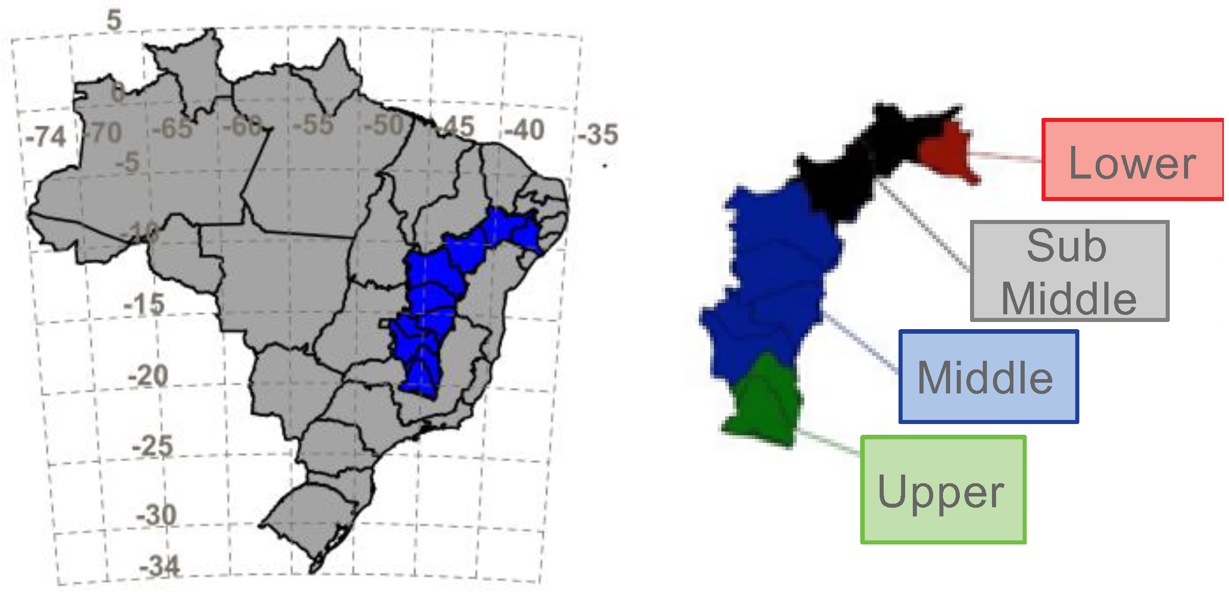
2.1. Study Area

The study area is the region of the Sao Francisco (SF) River basin (Figure 1). The SF River is one of Brazil’s major rivers. It is approximately 2700 km long and discharges an average flow of 2810 m³/s into the Atlantic Ocean [1]. Its watershed has an area of 639,219 km², characterized by different topographic and geomorphic features, and hosts a population of about 13 million people. This area is susceptible to droughts, which are recognized as potential environmental disasters and have attracted the attention of environmentalists, ecologists, hydrologists, meteorologists, geologists, and agricultural scientists [20]. By definition, droughts occur in virtually all climatic zones. They are mostly related to a reduction in the amount of precipitation received over an extended period, such as a season, a year, or multiple years [20].

The basin is commonly divided into four subbasins: upper, middle, submiddle, and lower (Figure 1). The lowest two river subbasins are located in Brazil’s semiarid “sertão” region, where dry periods can be prolonged and become droughts.

The Sao Francisco River basin allows multiple water uses, such as hydroelectricity, agriculture, navigation, fishing and aquaculture, human and industrial supply, flood control, recreation, and tourism. The wide variation in water availability throughout the basin and across the seasons, however, makes it difficult to plan efficient water allocation. Interannual variability in water availability may be partly related to climate variability, characterized by the occurrence of extremely rainy or dry years. There have been warnings concerning potential conflicts in this basin between the energy and agricultural sectors [21], such as the allocation of water from the Sobradinho reservoir for power generation and irrigation practices. The conflicts were aggravated, especially in the semiarid region, between 2011 and 2016, when rainfall in the basin was below normal amounts.

Although water availability in the basin is generally sufficient for multiple uses, the increasing demand for water resources leads to significant and occasional conflicts. According to Chiew (2006) [22], variability in river discharge and lake levels depends on variability in the intensity and accumulated volume of precipitation.

Different climate regimes are found in the Sao Francisco River basin (SF) due to its long north–south extension and topographic differences. In the upper SF, the climate varies from subtropical humid with dry winters and hot summers to temperate summers (Cwa and Cwb in Koppen’s classification). In the middle SF, a tropical climate with dry winters, Aw, predominates. The lower SF is predominately semiarid with some small patches of tropical, dry summers [4].

2.2. Eta Model

The Eta model is a grid-point limited-area model that represents the topography in steps, using the eta vertical coordinate [5]. The approximately horizontal surfaces of the eta coordinate reduce the errors in calculating horizontal derivatives near the topography, especially for the pressure gradient force. Such errors are commonly found in terrain-following coordinates in regions of steep topography. The Eta model is a comprehensive model with full dynamics and physics.

The model has received updates [6] to the operational version used initially at the National Centers for Environmental Prediction (NCEP) [7,8], which now include, for example, cut-cells. The model equations are solved on the Arakawa E-grid. The time integration is split explicit, using the forward–backward and Euler–backward schemes modified by Janjic (1979) [23]. The horizontal advection follows the Arakawa approach [24], and the vertical advection uses a piecewise linear scheme, which makes it a full finite-volume model. The model physics package of this version applies the Betts–Miller scheme [25] to produce convective precipitation and the Zhao scheme [26] for grid-scale precipitation. The longwave component of radiation is solved according to Schwarzkopf and Fels (1991) [27], and the shortwave component is solved according to Lacis and Hansen (1974) [28]. The surface layer is based on the Monin–Obukhov similarity theory and Paulson’s [29] stability functions. Land surface processes are treated using the NOAH scheme [30].

Eta model simulations on the subseasonal time range were generated for the 60-day integration, with a 20 km horizontal resolution. The model’s initial conditions were obtained from the Climate Forecast System Reanalysis (CFSR) [31]. The integrations started on 1 September and 1 January to evaluate the model’s accuracy at the onset and the middle of the rainy seasons in Brazil, respectively. These two simulation runs were referred to as the SO (September–October) and JF (January–February) runs. The first run contains the onset of the rainy season, and the second contains the middle of the rainy season.

2.3. Observational Data

As noted in Section 2.1, the SFRB is considered a large river basin. It is a challenge to obtain reliable and (temporally and spatially) consistent ground observations of the area for model evaluation. Therefore, remote sensing products are essential datasets for evaluating model performance. There are several remote sensing products that can be used to evaluate precipitation; the choice of the product to be used mainly depends on the study area and application of the data.

Lima et al. (2012) [32] showed the poor performance of satellite precipitation estimates over northeast Brazil, especially in estimating stratiform rainfall, which occurs frequently over northeast Brazil. Lima et al. (2012) [32] compared the Climate Prediction Center Morphing (CMORPH) products against other rainfall estimation methods for the summer periods (from December to February) between 2009 and 2011 in South America. They concluded that the models with the best performance were 3B42RT and CMORPH, mainly for south and southeast Brazil.

Laverde-Barajas et al. (2018) [33] evaluated the performance of near-real-time rainfall products to represent spatiotemporal characteristics of extreme events in a subtropical catchment in southeastern Brazil. CMORPH, PERSIANN-GCCS, TMPA-RT, and Hydro were compared against hourly rain gauge information during monsoon seasons from 2007 to 2014. The errors at different rainfall intensities, the performance in detecting different extreme events, and the sensitivity in the performance at different thresholds were analyzed, and the authors concluded that all products tended to overestimate rainfall within the study area, especially over elevated areas. CMORPH had the lowest quantitative error. The intensity of rainfall events has been found to strongly affect the performance of these products, as the bias increases with intensity.

In the analysis presented in this report, Eta precipitation simulations are compared against the CMORPH precipitation data. The CMORPH [34] data present a horizontal resolution of 8 km.

Despite the advantages of details provided by regional model simulations, systematic errors persist. These systematic errors may be associated with the forcing of the global climate model, in addition to errors inherent in the regional model’s representation of physical processes. The performance of subseasonal simulations is evaluated using metrics such as linear correlation, mean absolute error (MAE), and mean error (ME). These metrics are commonly used to evaluate climate models. The correlation describes the extent to which the simulation and the observed data are in agreement, so it is an important metric to take into account when analyzing the change in precipitation during the transitional months. The mean absolute error (MAE) provides the magnitude of departure in the simulation with respect to the observation, ignoring departure direction and not penalizing larger errors. Finally, the mean error (ME) provides what remains as a systematic error after cancellation between positive and negative errors. More information on these metrics can be found in the literature [35,36,37,38,39].

3. Results and Discussion

Simulations of precipitation variability over a 5-year mean were assessed. The mean of the 60-day simulation was discretized into 10-day simulations, referred to as periods D1, D2, D3, D4, D5, and D6, to evaluate intramonthly variations during the dry-to-wet transition (SO) and in the middle of the rainy season (JF).

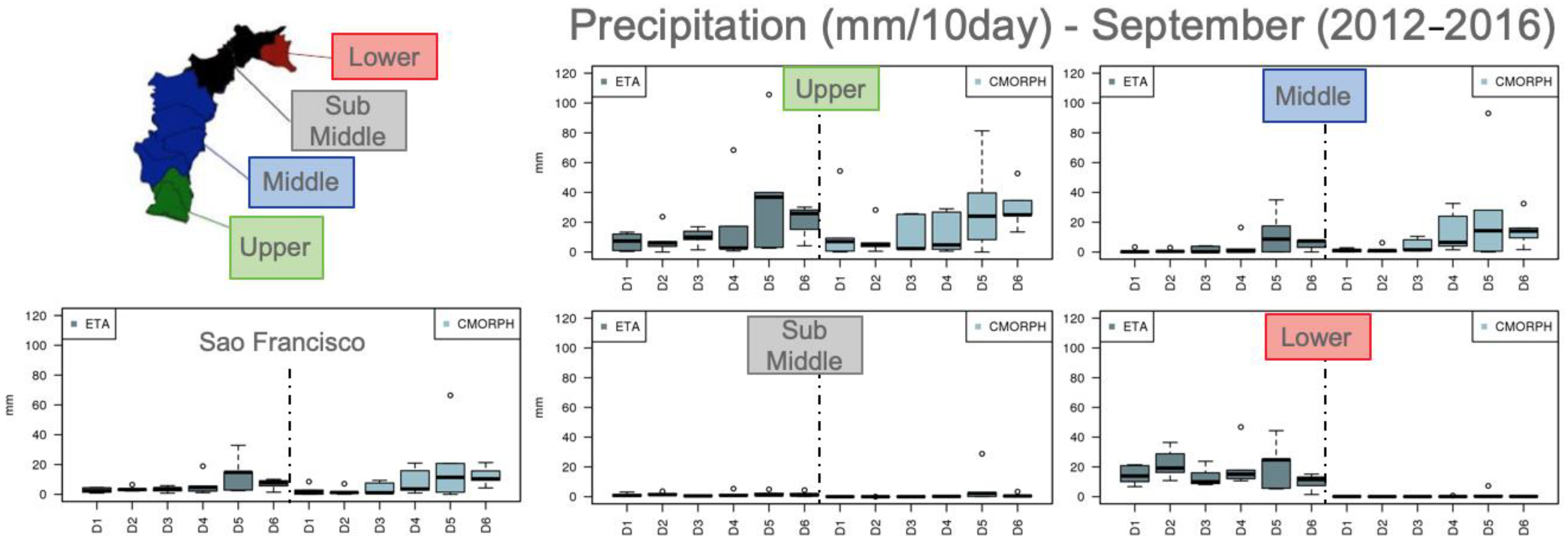
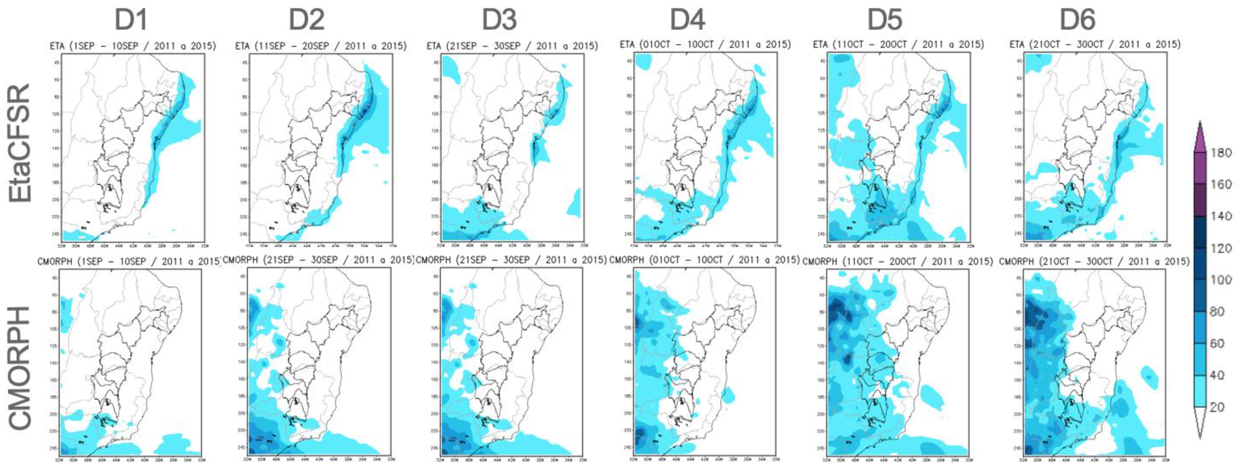
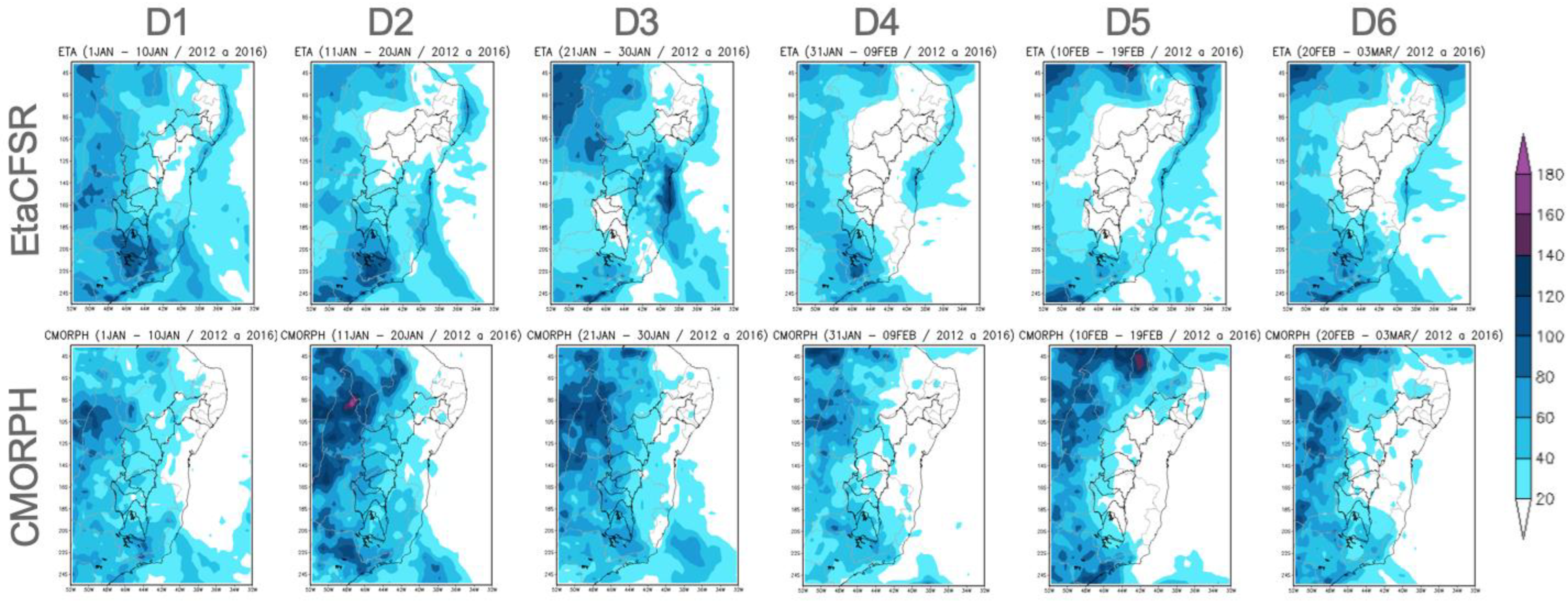
3.1. Precipitation Pattern

In SO, the Eta simulation results generally showed less precipitation when compared to CMORPH data for the SF River basin (Figure 2). However, in the lower SF, the Eta simulation showed precipitation in the northeastern Brazil coastal areas, where CMORPH data indicated little or no precipitation. This region is known as a region of high predictability. In the upper SF, the model introduced precipitation in D5, while CMORPH data showed precipitation from D2.

Over the Sao Francisco (SF) River basin, the JF simulations reproduced the CMORPH precipitation pattern, with larger accumulated amounts in the upper SF and lower SF (Figure 3). The JF simulation reproduced the precipitation pattern better than the SO simulation.

The presence in the simulation of precipitation on the northeast coast of Brazil may suggest an overestimation by the model. Owing to CMORPH’s limitations in estimating precipitation in northeast Brazil, other sources of data are considered for validating precipitation in this coastal area, especially for June and July, its rainy season.

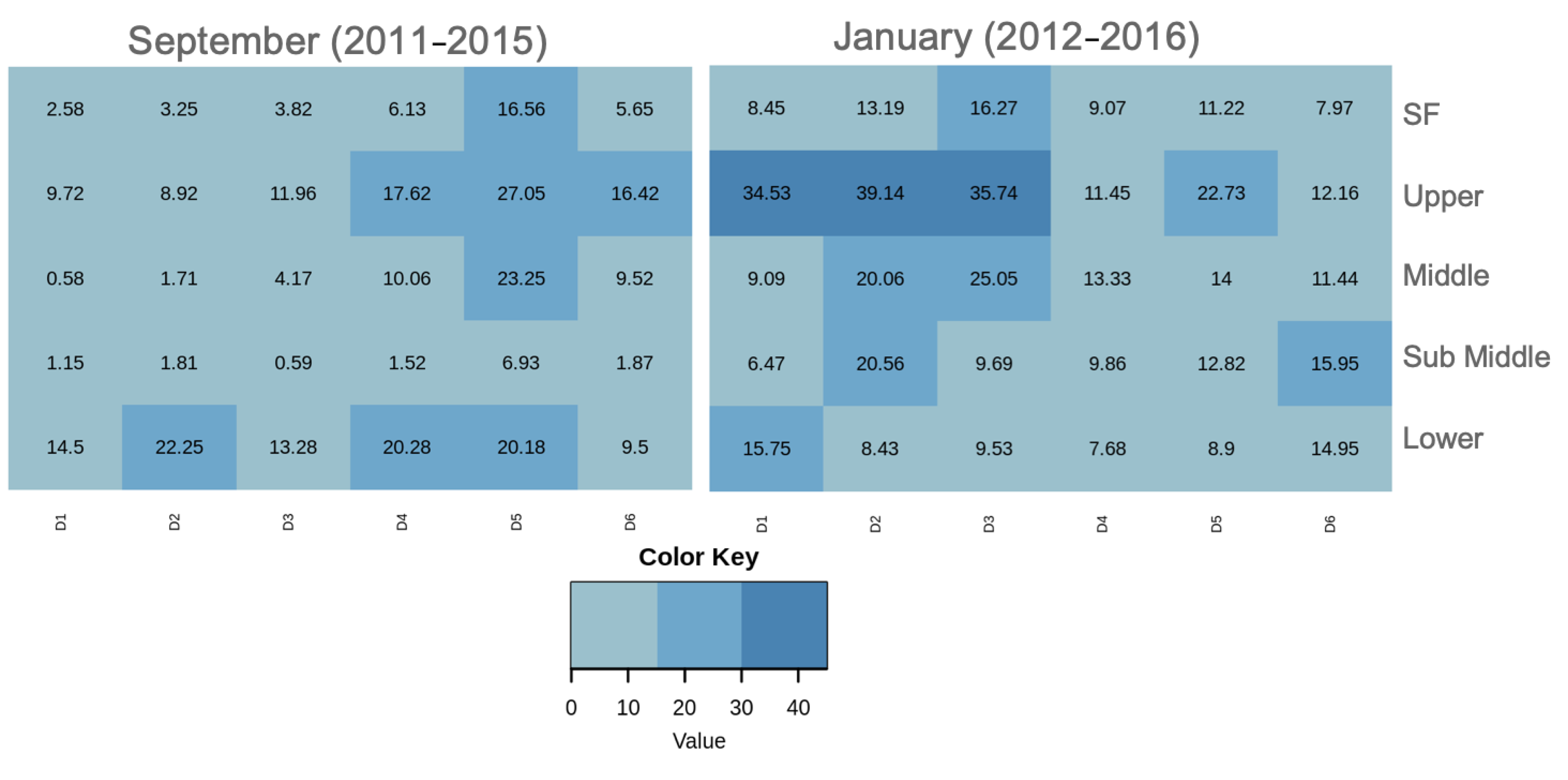
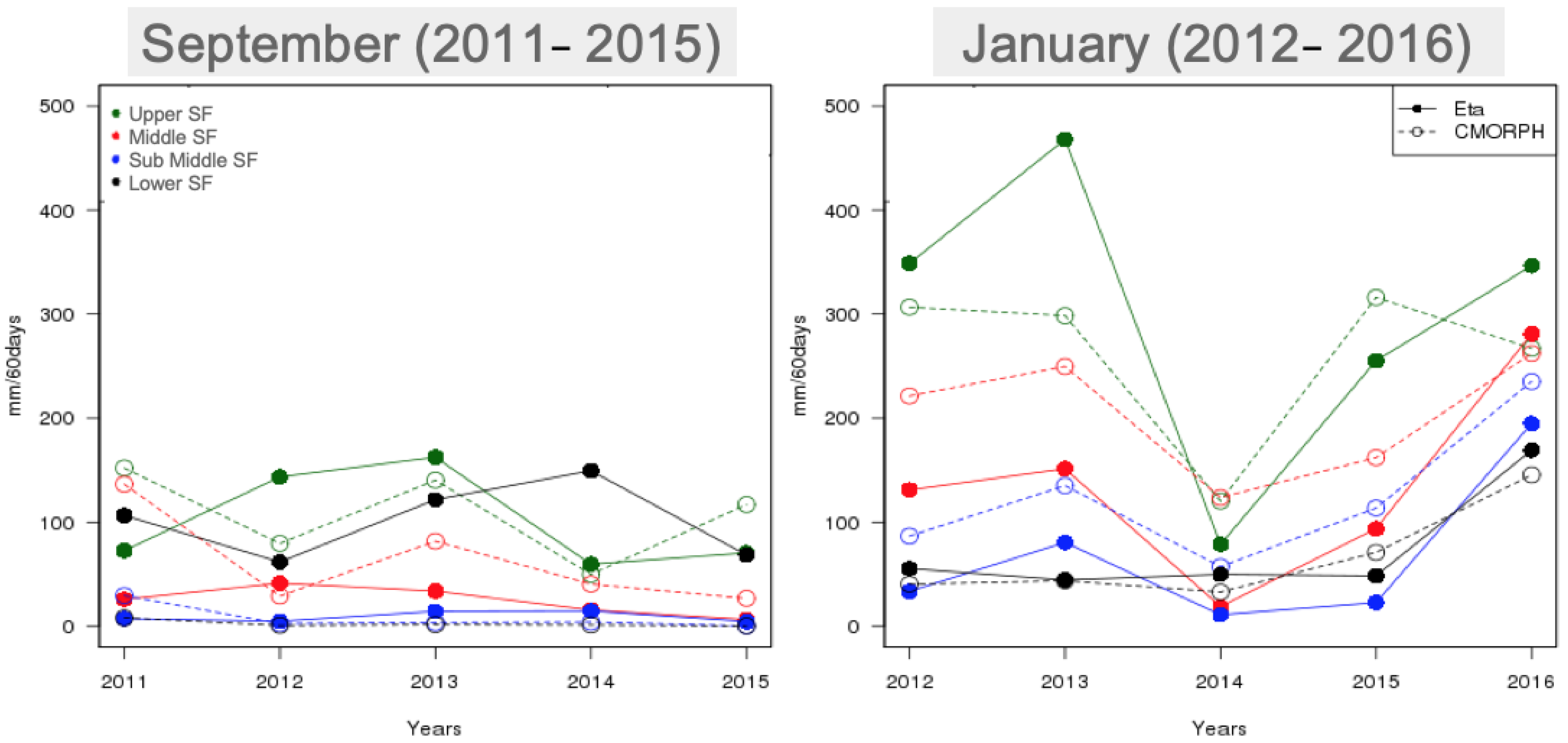
3.2. Interannual Variability

The performance of the Eta simulation was evaluated over the four major subbasins of the Sao Francisco (SF) river: the upper SF, middle SF, submiddle SF, and lower SF. Figure 4 shows the precipitation from the SO simulations, starting in September (2011 to 2015), and the JF simulations, starting in January (2012 to 2016).

In the SO simulations, the model approximately reproduced the decrease and increase in the magnitude of 60−day accumulated total precipitation. However, the simulation of the interannual variability was not well represented. The small amounts of precipitation in 2014 and 2015 hinted at the delay in the onset of the rainy season in these years. Both the Eta model and the CMORPH data indicated that the subbasin with the smallest rainfall volume was the submiddle SF. In the lower subbasin, CMORPH data showed no precipitation, but the model indicated amounts of about 100 mm/60 days. This overestimate is partly due to CMORPH’s limitations, as discussed in the previous section.

Both the SO runs and the CMORPH data indicated that the highest precipitation volumes occurred over the upper SF and the middle SF, and the lowest volumes occurred over the submiddle SF.

In the JF simulations, large precipitation volumes occurred during the middle of the rainy season. The JF simulations generally reproduced the interannual variability shown in the CMORPH estimates. The JF simulations captured the strong reduction in precipitation during 2014, when the rainfall was extremely far below the climatology rate [40,41]. The Eta simulations captured the precipitation decrease in 2014 and 2015 and the increase in 2016. The upper subbasin received the highest rainfall, while the submiddle received the lowest.

In the 60−day accumulations, the simulations performed better for the rainy months (JF) than for the transitional months from dry to wet (SO). In addition, the results showed the different precipitation regimes across the subbasins. These differences impose some difficulties on model simulations over the entire SF basin.

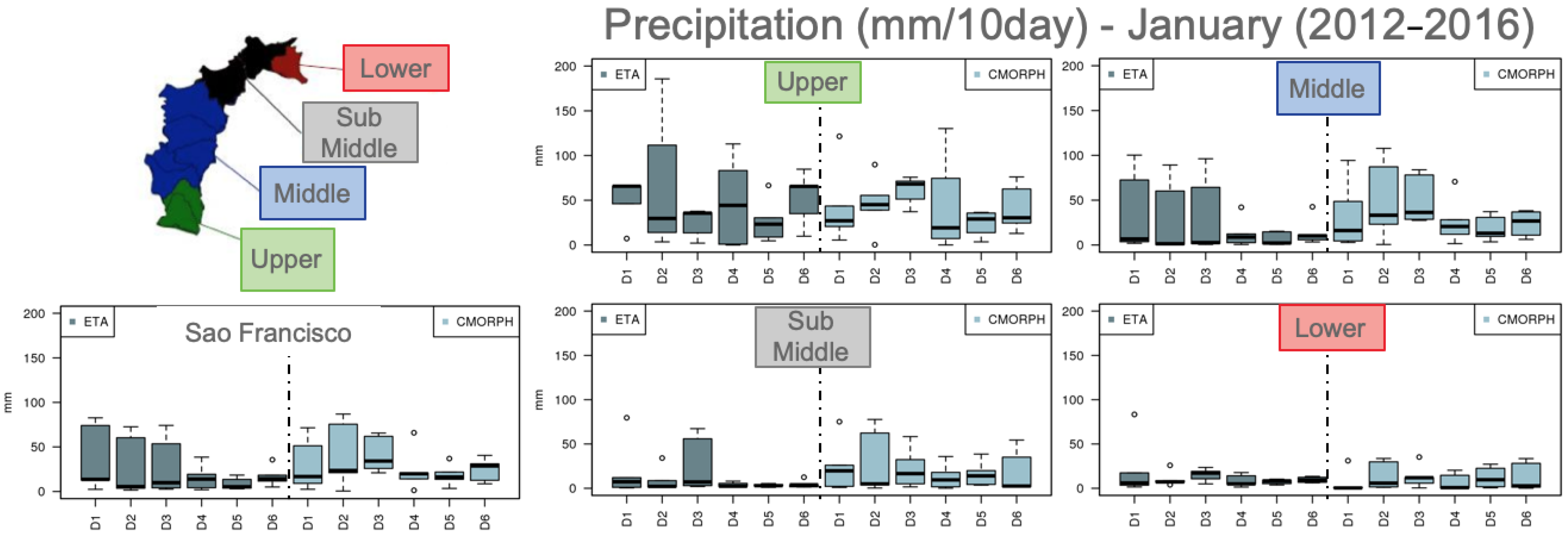
3.3. Intramonthly Variability

The intramonthly variability was observed through boxplots of accumulated precipitation for every 10−day period from the SO (Figure 5) and JF (Figure 6) simulations. Clearly, the JF simulations had higher precipitation amounts than the SO simulations.

In the upper SF, the SO simulations showed some limitations in representing the intramonthly variability in the first three 10−day simulations, D1, D2, and D3. On the other hand, these simulations correctly captured the variability in the last three 10−day simulations, D4, D5, and D6. The increase in the precipitation median in D5 and D6 in the upper and middle subbasins, shown by the CMORPH data, is the indication of the onset of the rainy season and was captured by the Eta simulations. The simulations also captured the lack of precipitation in all 10−day accumulations in the submiddle subbasin. However, for the lower subbasin, the simulation overestimated the precipitation, which may be a partial error from CMORPH data, as discussed previously.

In the middle SF, the JF simulations captured the large spread in precipitation between the 25th and 75th percentiles in D1–D3 and the decrease in the spread and amount of 10−day accumulated precipitation. However, in the submiddle SF, the simulations generally underestimated the accumulated precipitation, except for in D3, when the simulations overestimated the precipitation. The CMORPH data placed D2 as the rain peak, while the Eta simulations peaked in D3, which indicates a slight delay. Finally, despite underestimating the precipitation in the lower SF, the Eta simulations presented consistent values when compared to CMORPH data.

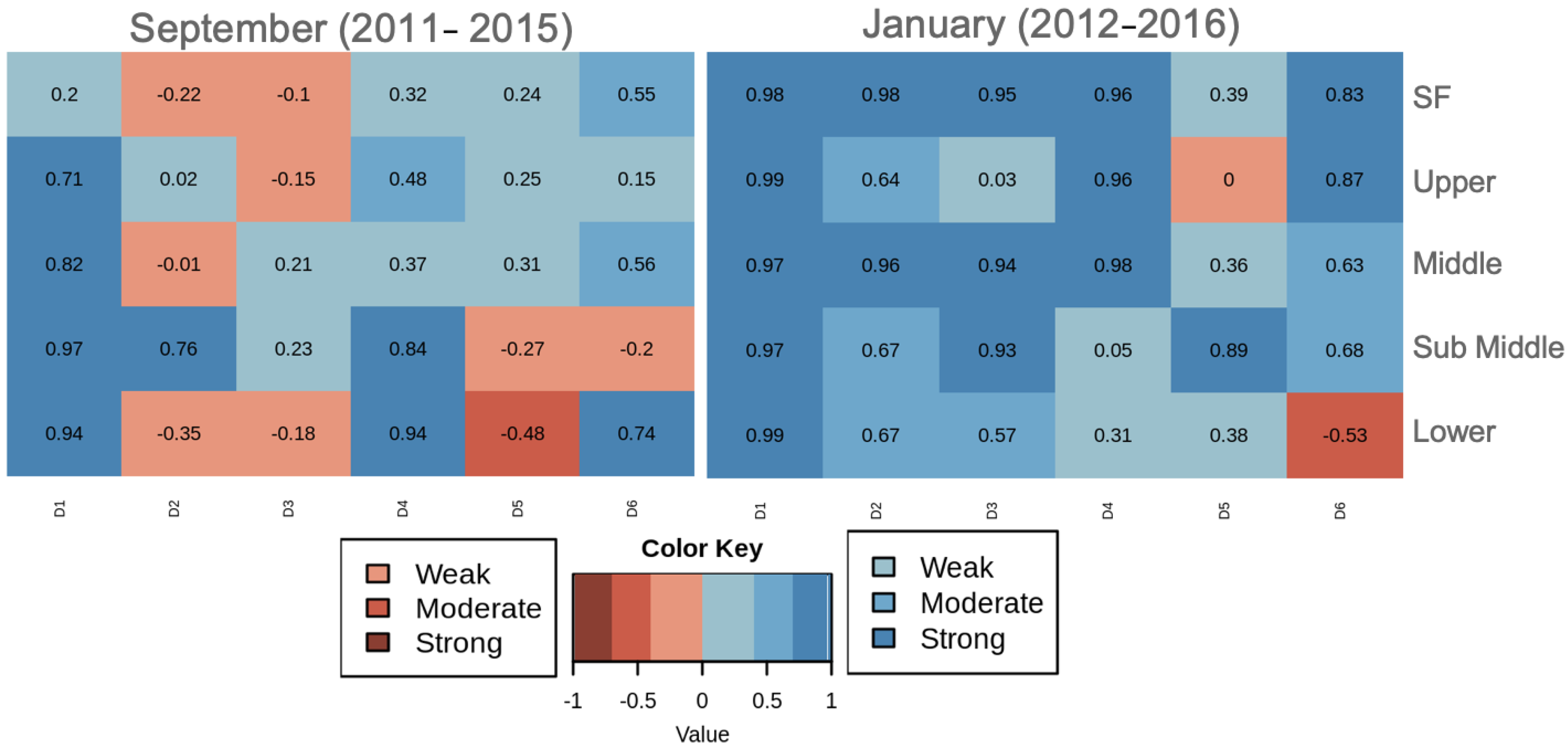
3.4. Simulation Accuracy

The Eta model’s capability to accurately simulate precipitation in the Sao Francisco basin was evaluated using the linear correlation (Figure 7), mean absolute error (Figure 8), and mean error (Figure 9).

The correlation between the Eta model results and CMORPH data can be classified as weak (0 to 0.4), moderate (0.4 to 0.7), or strong (0.7 to 1.0). The highest correlations between Eta and CMORPH precipitation were found in JF, rather than in SO (Figure 7). In SO, correlations became small or even negative from D2 onward. In the JF simulations, it was also observed that the Eta and CMORPH precipitation series were strongly to moderately correlated from D1 through D4. In both the SO and JF runs, the highest correlations were found in the middle SF. The model indicated difficulty in representing the lower SF, especially during the SO runs. This difficulty may be partly due to CMORPH’s limitations in this subbasin. The precipitation forecast accuracy is highly affected by the precipitation amount and by the size of the basin. Smaller basins generally present larger errors, as forecasts are more likely to miss the position of the precipitating system.

Although the correlation was low in SO simulations, the mean absolute error (MAE) values for precipitation were smaller in SO than in JF, given that the accumulated precipitation was smaller in SO than in JF (Figure 8). D5 was the 10−day simulation period with the highest MAE and the most significant rainfall in most of the subbasins. The MAE during D5 was 16.56 mm for the entire SF basin and up to 27.05 mm for the upper SF. In JF, the highest MAE values were found in D2 and D3, the periods with the most significant rainfall. For example, the highest MAE was 39.14 mm for the upper SF in D2.

Mean error (ME) estimates were assessed to indicate whether simulations overestimated or underestimated precipitation in each subbasin and across different simulations (Figure 9).

Considering the entire SF basin, the SO simulations overestimated precipitation in D1 and D2 and underestimated it in D3, D4, D5, and D6. The precipitation simulations for the middle SF contributed mostly to the underestimation for the entire SF basin. In contrast, the precipitation simulations for the submiddle and lower SF contributed to overestimation for the entire basin from D1 to D6, generally. Overall, the largest ME in the SO simulation occurred in D5 for the submiddle SF. However, in D6, errors decreased, indicating usefulness in this range of the simulation.

In the JF simulations, the ME indicated an underestimation of precipitation over the SF basin, except in D1. As in SO, in JF, the middle SF contributed significantly to the overall underestimation. For the upper SF, precipitation was generally overestimated, especially in D1, with errors reaching 34.53 mm. Precipitation was mostly underestimated for the submiddle subbasin and slightly less so for the lower SF.

In the results presented, subseasonal simulations for the SF basin showed limitations in the transitional months. Some aspects that may contribute to these model errors are the complex topography, heterogeneous vegetation, and general climate conditions in the river basin. Generally, precipitation in the upper and middle SF subbasins was better simulated, although it still exhibited relatively large errors.

The accuracy of a forecast is highly associated with the season, the amount of precipitation, and the size of the subbasin. Because of the relatively small size of the lower and upper subbasins, these were also the subbasins with higher errors in the simulation. On the other hand, as the upper subbasin experiences more precipitation in JF, this tended to be the subbasin with larger errors.

4. Conclusions

Five−year mean subseasonal simulations were generated using the Eta model driven by CFSR conditions. The simulated 60−day periods started in September (SO, averaged over 2011 to 2015) and January (JF, averaged over 2012 to 2016), and they were assessed by discretization into six 10−day precipitation outputs.

In the SO runs, the precipitation volumes in the Eta model simulations were lower than those in the CMORPH data. However, Eta simulations indicated precipitation in the lower SF, a coastal region, where CMORPH data indicated little or no precipitation. In the upper SF, the Eta model showed rain from D3, while CMORPH data showed rain from D1, which revealed the model’s difficulty in representing precipitation in the transitional months. As expected, the SO runs showed the model’s limited ability to reproduce precipitation during this transitional period.

In the 10−day simulations, the Eta model produced higher precipitation rates in the upper and lower SF, while CMORPH data showed higher precipitation rates in the upper and middle SF. Both Eta and CMORPH data showed maximum rainfall at D5 as an indication of the onset of the rainy season. Considering the entire SF basin, the simulations reproduced the rainfall distribution over the 60−day simulated period.

Despite the low correlation, the SO runs had a small MAE due to the small precipitation volume. Considering the entire SF basin, the Eta model overestimated rainfall in D1 and D2 and underestimated it in D3, D4, D5, and D6. However, errors varied strongly across the basin. In the middle SF, precipitation was underestimated, while it was overestimated in the lower SF.

In the JF simulations, precipitation was overestimated in the lower SF, on the northeast coast, while CMORPH showed no precipitation. However, in the upper SF, the Eta simulations showed a similar rainfall distribution to CMORPH, with higher precipitation values. The JF simulations reproduced the annual variability better than the SO simulations.

Both Eta and CMORPH data indicated that, in the SF basin, the highest rainfall occurred in the first three 10−day simulations, D1, D2, and D3. In the upper SF, the model showed limitations in the first three 10-day simulations but then showed good simulation capability for the last three. In the middle SF, the Eta model reproduced the CMORPH precipitation distribution pattern well, with the highest precipitation values occurring in the first three 10-day simulations. In the lower SF, although underestimated, the precipitation simulated by the Eta model was consistent with that from CMORPH data. The highest correlation values were found in the JF simulations. The highest correlations and the smallest MAE were generally found in D1 and D4. A variable error pattern was identified for the upper SF, with overestimation and underestimation according to the 10-day simulations, while in the other three subbasins, underestimation was identified. The largest ME was found in the JF simulations, which correspond to months of higher rainfall compared to the SO simulations.

The present research contributed an assessment of subseasonal-scale simulations using a regional climate model. This type of assessment has been more extensively applied to global climate models. The Eta model simulations showed good performance at this scale. However, there were some limitations in the assessment that should be kept in mind. The evaluation was based on CMORPH data, which have a higher resolution than the simulation model. For this reason, some extreme events may not have been properly simulated. In addition, the study region where the SF basin is located has low predictability.

Further modeling studies are required, including updated soil maps, vegetation, and adjustments to rainfall production. Future studies will incorporate these improvements, and bias removal may also be included. Therefore, this research is a critical step to indicate subbasins where the model simulation needs to be improved and provide initial information to support water allocation in the region.

References

1. Filho, J.G.G.; Formiga, K.T.; Duarte, R.X.; Sugai, M.R. Análise da Cheia de 2004 na Bacia do Rio São Francisco. In Proceedings of the Simpósio Brasileiro de Desastres Naturais, Florianopolis, Brazil, 27–30 September 2004. [Google Scholar]
2. Rodwell, M.J.; Doblas-Reyes, F.J. Medium-range, monthly, and seasonal prediction for Europe and the use of forecast information. J. Clim. 2006, 19, 6025–6046. [Google Scholar] [CrossRef]
3. Vitart, F.; Ardilouze, C.; Bonet, A.; Brookshaw, A.; Chen, M.; Codorean, C.; Déqué, M.; Ferranti, L.; Fucile, E.; Fuentes, M.; et al. The subseasonal to seasonal (S2S) prediction project database. Bull. Am. Meteorol. Soc. 2017, 98, 163–173. [Google Scholar] [CrossRef]
4. Alvares, C.A.; Stape, J.L.; Sentelhas, P.C.; Gonçalves, J.L.M.; Sparovek, G. Köppen’s climate classification map for Brazil. Meteorol. Z. 2013, 22, 711–728. [Google Scholar] [CrossRef] [PubMed]
5. Mesinger, F. A blocking technique for representation of mountains in atmospsheric models. Riv. Meteor. Aeronaut. 1984, 44, 195–202. [Google Scholar]
6. Mesinger, F.; Chou, S.; Gomes, J.; Jovic, D.; Lazic, L.; Lyra, A.; Ristic, I. An Upgraded Version of the Eta Model; European Geosciences Union (EGU) General Assembly: Munich, Germany, 2011; p. 2011. [Google Scholar]
7. Black, T.L. The new NMC mesoscale Eta model: Description and forecast examples. Weather. Forecast. 1994, 9, 265–278. [Google Scholar] [CrossRef]
8. Mesinger, F.; Janjić, Z.I.; Ničković, S.; Gavrilov, D.; Deaven, D.G. The step-mountain coordinate: Model description and performance for cases of Alpine lee cyclogenesis and for a case of an Appalachian redevelopment. Mon. Weather. Rev. 1988, 116, 1493–1518. [Google Scholar] [CrossRef]
9. Chou, S.C.; Ferreira, N.C.R.; Rocha, M.L.; Gomes, J.L.; Dereczynski, C.; Sueiro, G. From subseasonal to seasonal forecasts over South America using the Eta Model. In Numerical Weather and Climate Modeling: Beginning, Now, and Vision of the Future; Cambridge University Press: Cambridge, UK, 2018. [Google Scholar]
10. Seluchi, M.E.; Chou, S.C. Evaluation of two Eta Model versions for weather forecast over South America. Geofísica Int. 2001, 40, 219–237. [Google Scholar] [CrossRef]
11. Seluchi, M.E.; Chou, S.C. Synoptic patterns associated with landslide events in the Serra do Mar, Brazil. Theor. Appl. Clim. 2009, 98, 67–77. [Google Scholar] [CrossRef]
12. Seluchi, M.E.; Chou, S.C.; Gramani, M. A case study of a winter heavy rainfall event over the Serra do Mar in Brazil. Geofísica Int. 2011, 50, 41–56. [Google Scholar] [CrossRef]
13. Siqueira, V.A.; Collischonn, W.; Fan, F.M.; Chou, S.C. Ensemble flood forecasting based on operational forecasts of the regional Eta EPS in the Taquari-Antas basin. Rev. Bras. Recur. Hídricos 2016, 21, 587–602. [Google Scholar] [CrossRef]
14. Pilotto, I.L.; Chou, S.C.; Nobre, P. Seasonal climate hindcasts with Eta model nested in CPTEC coupled ocean–atmosphere general circulation model. Theor. Appl. Clim. 2012, 110, 437–456. [Google Scholar] [CrossRef]
15. Bustamante, J.F.; Gomes, J.L.; Chou, S.C. 5-Years Eta Model Seasonal Forecast Climatology over South America; CSHMO: Foz do Iguaçu, Brazil, 2006. [Google Scholar]
16. Weber, T.M.; Dereczynski, C.P.; dos Santos Souza, R.H.; Chou, S.C.; Bustamante, J.F.; de Paiva Neto, A.C. Investigação da Previsibilidade Sazonal da Precipitação na Região do Alto São Francisco em Minas Gerais. Anuário Inst. Geociências 2016, 38, 24–36. [Google Scholar] [CrossRef]
17. Resende, N.; Chou, S.C. Influência das condições do solo na climatologia da previsão sazonal do modelo ETA. Rev. Bras. Climatol. 2015, 15. [Google Scholar] [CrossRef]
18. Ferreira, N.C.R.; Chou, S.C. Influência do tipo de textura e umidade inicial do solo sobre a simulação da precipitação sazonal e de extremos de precipitação no sudeste do Brasil. Anuário Inst. Geociências 2018, 41, 680–689. [Google Scholar] [CrossRef]
19. Bombardi, R.J.; Moron, V.; Goodnight, J.S. Detection, variability, and predictability of monsoon onset and withdrawal dates: A review. Int. J. Clim. 2019, 40, 641–667. [Google Scholar] [CrossRef]
20. Mishra, A.K.; Singh, V.P. review of drought concepts. J. Hydrol. 2010, 391, 202–216. [Google Scholar] [CrossRef]
21. ANA. PAE: Programa de Ações Estratégicas Para O Gerenciamento Integrado da Bacia do Rio São Francisco e da Sua Zona Costeira; GEF São Francisco: Relatório Final, Brasília, 2004. [Google Scholar]
22. Chiew, F.H. Estimation of rainfall elasticity of streamflow in Australia. Hydrol. Sci. J. 2006, 51, 613–625. [Google Scholar] [CrossRef]
23. Janjic, Z.I. Forward-backward scheme modified to prevent two-grid-interval noise and its application in sigma coordinate models. Contrib. Atmos. Phys. 1979, 52, 69–84. [Google Scholar]
24. Janjić, Z.I. Nonlinear advection schemes and energy cascade on semi-staggered grids. Mon. Weather. Rev. 1984, 112, 1234–1245. [Google Scholar] [CrossRef]
25. Betts, A.K.; Miller, M.J. A new convective adjustment scheme. Part II: Single column tests using GATE wave, BOMEX, ATEX and arctic air-mass data sets. Q. J. R. Meteorol. Soc. 1986, 112, 693–709. [Google Scholar]
26. Zhao, Q.; Carr, F.H. A prognostic cloud scheme for operational NWP models. Mon. Weather. Rev. 1997, 125, 1931–1953. [Google Scholar] [CrossRef]
27. Schwarzkopf, M.D.; Fels, S.B. The simplified exchange method revisited: An accurate, rapid method for computation of infrared cooling rates and fluxes. J. Geophys. Res. Atmos. 1991, 96, 9075–9096. [Google Scholar] [CrossRef]
28. Lacis, A.A.; Hansen, J. A parameterization for the absorption of solar radiation in the earth’s atmosphere. J. Atmospheric Sci. 1974, 31, 118–133. [Google Scholar] [CrossRef]
29. Paulson, C.A. The mathematical representation of wind speed and temperature profiles in the unstable atmospheric surface layer. J. Appl. Meteorol. 1970, 9, 857–861. [Google Scholar] [CrossRef]
30. Ek, M.B.; Mitchell, K.E.; Lin, Y.; Rogers, E.; Grunmann, P.; Koren, V.; Gayno, G.; Tarpley, J.D. Implementation of Noah land surface model advances in the National Centers for Environmental Prediction operational mesoscale Eta model. J. Geophys. Res. Atmos. 2003, 108. [Google Scholar] [CrossRef]
31. Saha, S.; Moorthi, S.; Pan, H.L.; Wu, X.; Wang, J.; Nadiga, S.; Tripp, P.; Kistler, R.; Woollen, J.; Behringer, D.; et al. The NCEP climate forecast system reanalysis. Bull. Am. Meteorol. Soc. 2010, 91, 1015–1058. [Google Scholar] [CrossRef]
32. Lima, W.F.; Vendrasco, E.P.; Vila, D. Desempenho dos Modelos de Estimativa de Precipitação Por Satélite No Inverno/Verão no América do Sul. 2012. Available online: https://www.researchgate.net/profile/Wagner-Lima-6/publication/281824477_Desempenho_dos_Modelos_de_Estimativa_de_Precipitacao_por_Satelite_no_InvernoVerao_na_America_do_Sul/links/55f9a47308aeafc8ac26ef38/Desempenho-dos-Modelos-de-Estimativa-de-Precipitaca (accessed on 10 August 2023).
33. Laverde-Barajas, M.; Perez, G.C.; Filho, J.D.; Solomatine, D. Assessing the performance of near real-time rainfall products to represent spatiotemporal characteristics of extreme events: Case study of a subtropical catchment in south-eastern Brazil. Int. J. Remote. Sens. 2018, 39, 7568–7586. [Google Scholar] [CrossRef]
34. Joyce, R.J.; Janowiak, J.E.; Arkin, P.A.; Xie, P. CMORPH: A method that produces global precipitation estimates from passive microwave and infrared data at high spatial and temporal resolution. J. Hydrometeorol. 2004, 5, 487–503. [Google Scholar] [CrossRef]
35. Nice, K.A.; Coutts, A.M.; Tapper, N.J. evelopment of the VTUF-3D v1. 0 urban micro-climate model to support assessment of urban vegetation influences on human thermal comfort. Urban Clim. 2018, 24, 1052–1076. [Google Scholar] [CrossRef]
36. Lorenz, C.-L.; Packianather, M.; Spaeth, A.B.; De Souza, C.B. Artificial Neural Network-Based Modelling for Daylight Evaluations; SimAUD: Delft, The Netherlands, 2018. [Google Scholar]
37. Shu, C.; Gaur, A.; Wang, L.; Bartko, M.; Laouadi, A.; Ji, L.; Lacasse, M. Added value of convection permitting climate modelling in urban overheating assessments. Build. Environ. 2022, 207, 108–415. [Google Scholar] [CrossRef]
38. Chakraborty, D.; Dobor, L.; Zolles, A.; Hlásny, T.; Schueler, S. High-resolution gridded climate data for Europe based on bias-corrected EURO-CORDEX: The ECLIPS dataset. Geosci. Data J. 2021, 8, 121–131. [Google Scholar] [CrossRef]
39. Resende, N.C.; Miranda, J.H.; Cooke, R.; Chu, M.L.; Chou, S.C. Impacts of regional climate change on the runoff and root water uptake in corn crops in Parana, Brazil. Agric. Water Manag. 2019, 221, 556–565. [Google Scholar] [CrossRef]
40. Marengo, J.A.; Cunha, A.P.; Alves, L.M. A seca de 2012-15 no semiárido do Nordeste do Brasil no contexto histórico. Rev. Climanálise 2016, 3, 49–54. [Google Scholar]
41. Marengo, J.A.; Alves, L.M. Crise hídrica em São Paulo em 2014: Seca e desmatamento. GEOUSP Espaço Tempo (Online) 2015, 19, 485–494. [Google Scholar] [CrossRef]
Figure 1. São Francisco River basin (Brazil) and its four subbasins: upper, middle, submiddle, and lower.
Climate 11 00213 g001
Figure 2. Ten-day accumulated precipitation, starting from 1 September, averaged over 2011 to 2015: Eta model simulation (top row); and CMORPH observed data (bottom). The 60-day simulations were discretized into 10-day periods, referred to as D1, D2, D3, D4, D5, and D6.
Climate 11 00213 g002
Figure 3. Ten-day accumulated precipitation, starting from 1 January, averaged over 2012 to 2016: Eta model simulation (top row); and CMORPH observed data (bottom). The 60-day simulations were discretized into 10-day periods, referred to as D1, D2, D3, D4, D5, and D6.
Climate 11 00213 g003
Figure 4. Sixty−day accumulated precipitation (mm/60 days) starting in September (left) and starting in January (right). The Eta simulations are shown as solid lines and full dots. The CMORPH data are shown as dotted lines. Average rainfall is indicated by green lines for the upper SF subbasin, red for the middle subbasin, blue for the submiddle subbasin, and black for the lower Sao Francisco subbasin.
Climate 11 00213 g004
Figure 5. Boxplots showing the 10−day accumulated precipitation (D1, D2, D3, D4, D5, and D6) for the September and October period, averaged over 2011–2016, in the different subbasins of the Sao Francisco River. The Eta simulations are the six leftmost bars in gray, and the CMORPH data are the six rightmost bars in blue.
Climate 11 00213 g005
Figure 6. Boxplots showing the 10−day accumulated precipitation (D1, D2, D3, D4, D5, and D6) for the January and February period, averaged over 2011–2016, in the different subbasins of the Sao Francisco River. The Eta simulations are the six leftmost bars in gray, and the CMORPH data are the six rightmost bars in blue.
Climate 11 00213 g006
Figure 7. Linear correlations between the Eta model simulations and CMORPH precipitation in each subbasin of the SF basin and for each 10−day period. Red indicates negative correlations, and blue indicates positive correlations. Correlations are divided into weak (0 to 0.4), moderate (0.4 to 0.7), and strong (0.7 to 1).
Climate 11 00213 g007
Figure 8. Mean absolute error (MAE) values for the Eta model precipitation simulations in each subbasin of the SF basin and for every 10−day period.
Climate 11 00213 g008
Figure 9. Mean error (ME) for the Eta model simulations in each subbasin of the Sao Francisco River basin. Red indicates negative biases, and blue indicates positive biases.
Climate 11 00213 g009
Disclaimer/Publisher’s Note: The statements, opinions and data contained in all publications are solely those of the individual author(s) and contributor(s) and not of MDPI and/or the editor(s). MDPI and/or the editor(s) disclaim responsibility for any injury to people or property resulting from any ideas, methods, instructions or products referred to in the content.