Article

A Methodology for Bridging the Gap between Regional- and City-Scale Climate Simulations for the Urban Thermal Environment

by
Konstantina Koutroumanou-Kontosi
,
Constantinos Cartalis
*,
Kostas Philippopoulos
,
Ilias Agathangelidis
and
Anastasios Polydoros
Department of Physics, National and Kapodistrian University of Athens, 15784 Athens, Greece
*
Author to whom correspondence should be addressed.
Climate 2022, 10(7), 106; https://doi.org/10.3390/cli10070106
Submission received: 29 May 2022 / Revised: 3 July 2022 / Accepted: 11 July 2022 / Published: 13 July 2022
(This article belongs to the Topic Urban Mitigation and Adaptation to Climate Change)

Abstract

:
The main objective of this study is to bridge the gap between regional- and city-scale climate simulations, with the focus given to the thermal environment. A dynamic-statistical downscaling methodology for defining daily maximum (Tmax) and minimum (Tmin) temperatures is developed based on artificial neural networks (ANNs) and multiple linear regression models (MLRs). The approach involves the use of simulations from two EURO-CORDEX regional climate models (RCMs) (at approximately 12 km × 12 km) that are further downscaled to a finer resolution (1 km × 1 km). A feature selection methodology is applied to select the optimum subset of parameters for training the machine learning models. The downscaling methodology is initially applied to two RCMs, driven by the ERA-Interim reanalysis (2008–2011) and high-resolution urban climate model simulations (UrbClims). The performance of the relationships is validated and found to successfully simulate the spatiotemporal distribution of Tmax and Tmin over Athens. Finally, the relationships that were extracted by the models are further used to quantify changes for Tmax and Tmin in high resolution, between the historical period (1971–2000) and mid-century (2041–2071) climate projections for two different representative concentration pathways (RCP4.5 and RCP8.5). Based on the results, both mean Tmax and Tmin are estimated to increase by 1.7 °C and 1.5 °C for RCP4.5 and 2.3 °C and 2.1 °C for RCP8.5, respectively, with distinct spatiotemporal patterns over the study area.

1. Introduction

Long-term observational records provide ample evidence of an increase in the mean global air temperature due to anthropogenic climate change [1]. Additionally, in recent years an unusual frequent number of record-shattering temperature extremes, often accompanied by heat-related mortality [2], have been observed. These extreme weather events are projected to increase in intensity and recurrence [3,4], becoming up to seven times more probable within the next 30 years [5]. The impact of excessive heat is expected to be more severe in urban areas as it adds to the existing warming from the urban heat island (UHI) effect [6]. The lack of appropriate frameworks and high-quality data is a crucial aspect that limits climate-informed decision-making. The urban environment is characterized by high heterogeneity with different types of land use. High-frequency and complex transitions of urban characteristics (e.g., building height, imperviousness density, canyon aspect ratio) pose the need for high-resolution data in order to define the intra-urban vulnerability to climate change and, subsequently, to introduce spatially focused adaptation and mitigation measures. For instance, although urban flooding is an inevitable natural hazard [7], climate information can provide the required level of scientific evidence for drafting flood adaptation/mitigation measures that can lead to efficient management. Furthermore, high ambient temperatures and heat waves cause adverse impacts on human health [8]; however, their intra-urban variability introduces different magnitudes of exposure and, hence, the lack of high-resolution data leads to insufficient public decision measures. Moreover, excessive urban heat influences the energy demand of buildings (increased for cooling and decreased for heating) [9]. Thus, solutions such as building renovations and retrofitting can contribute to reducing energy consumption through energy efficiency upgrades, but without data at a finer resolution, their prioritization would not be optimum.
Hence, cities are characterized as hotspots of climate change impacts and risks and the proposed methodology can contribute to limiting the uncertainties related to the intra-urban variability of air temperature. Improved high-resolution climate projections for the urban thermal environment are of great relevance, taking into account the need for developing adaptation measures.
Global circulation models (GCMs) simulate the Earth’s climate via mathematical equations that describe atmospheric, oceanic, and biotic processes, interactions, and their feedbacks [10]. GCMs provide future climate scenarios at a coarse spatial and temporal resolution, and, therefore, their results are inadequate for use in climate impact models. As a consequence, the need for higher-resolution data that can be used for regional and local studies led to the development of different downscaling methods [11]. There are mainly two downscaling approaches, the “dynamic” and the “statistical”.
The first approach relies on the use of a regional climate model (RCM), which is nested within a GCM and covers a limited spatial domain. The reduction of the simulated area allows the introduction of more detailed descriptions of physical processes and surface topography and, hence, generates more realistic climate information [12]. Since the RCM is driven by the GCM output, its overall quality is directly related to the biases of the latter one (Storch and Chen, 2001). A single RCM will probably not provide “accurate” results and, thus, projects that utilize various RCMs driven by multiple GCMs from the Coupled Model Intercomparison Project Phases have been developed to produce multi-model ensembles of regional-scale projections. The EURO-CORDEX framework oversees the design and coordination of ongoing ensembles of climate projections for the region of Europe at a spatial resolution of 0.11° (EUR-11) and 0.44° (EUR-44) [13].
Even though RCMs have a significantly finer resolution than GCMs, locally focused studies, such as species distribution, forest growth, and ecosystem modeling studies, require higher-resolution data [14,15]. However, local factors are not resolved by even the finest RCMs [16] and, consequently, further downscaling is necessary to include more detailed information about coastal, orographic, and land-use features to capture local-scale processes.
As far as urban areas are concerned, their specific characteristics such as the high heterogeneity of the surfaces in combination with their size require the performance of high-resolution models since the detailed representation of the land cover and its physical properties are crucial for impact studies [17]. Downscaling RCM outputs to an urban scale provides useful information on climate change scenarios and, therefore, contributes to the development of adaptation planning and mitigation strategies by the city planners.
The second approach includes statistical downscaling (SD) methods [18] aiming to bridge the gap between large and local scales and establish empirical relations between coarse-resolution predictors and smaller-scale historical observations of the climate variable of interest (predictand). A vast number of SD techniques have been developed [19]; a common assumption for all is that the currently observed relationships will be upheld in the future, i.e., that a stationary statistical relationship exists. Depending on the nature of predictors, observed or simulated, SD is divided into two further subcategories: (a) perfect prognosis (PP) [20,21,22] and (b) model output statistics (MOS) [18,23,24].
Under PP, the statistical link is typically calibrated between daily quasi-observed data from reanalysis datasets (predictors) and the simultaneously observed predictand. To infer the statistical relationship, a suitable choice of predictors should include large-scale variables that account for a high proportion of the variability of the predictand and are well presented by both reanalysis and climate models [19,25].
Conversely to PP, MOS derives local-scale climatic information linking model-simulated features to the target variable. An important advantage of MOS is the ability to explicitly account for model-inherent biases and errors [26]. As most simulation outputs are typically generated with a free-running GCM or a GCM-driven RCM experiment, MOS methods are usually limited to calibrations based on long-term distributions of the climate variables [27]. Nevertheless, using GCM outputs nudged to reanalysis [25] or reanalysis-driven historical RCM simulations, MOS can also be applied in an event-wise context similar to that of PP [26,28]. For both distribution-wise and event-wise cases, MOS relations are specific only to the climate model upon which they have been established.
For urban areas, a wide range of downscaling methodologies were recently proposed in order to derive future climatic conditions with improved detail and accuracy. Dynamical downscaling of GCMs through nested RCMs was found to provide added value to urban areas, especially for coastal cities; however, important urban thermal dynamic processes are not sufficiently captured [29,30]. A full dynamical approach from the global scale down to the urban scale [31], albeit the most physically valid and consistent methodology, is usually not preferred, given its considerable computational cost [32].
Hence, both SD methods of PP [33,34] and MOS [35,36,37,38] are widely common for urban areas, with the latter typically applied as a quantile mapping bias correction. Simple SD methods largely lack, however, the ability to represent the intra-urban variability of urban areas or to capture complex interactions [32]. Therefore, a hybrid statistical-dynamical downscaling (SDD) scheme is increasingly being employed in order to make best use of the respective benefits of each individual approach [17,32,39,40,41,42]. To accomplish this, a fine-scale simulation is initially conducted for the urban area under consideration, commonly for a relative short temporal period, the output of which is subsequently combined with large-scale GCM or RCM projections to provide downscaled urban climatic information.
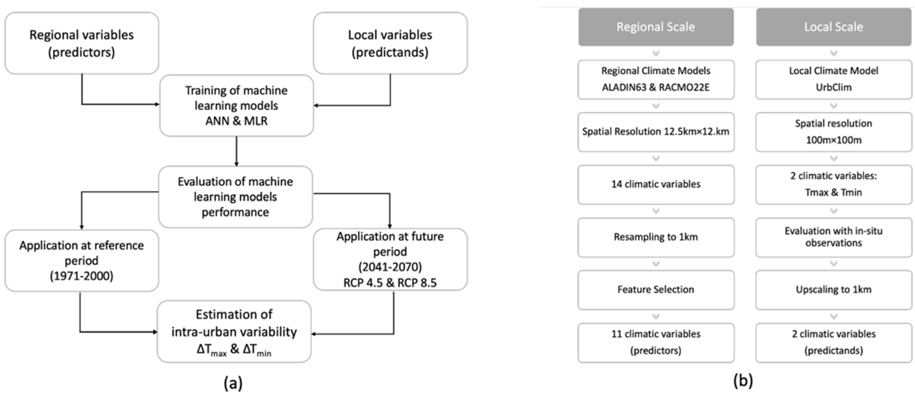
This paper aims to bridge the gap between the regional climate model resolution (approximately 12 km) and the respective one at the local scale for improving the climate projections of the urban thermal environment. This work proposes an easily replicable data-driven workflow and a hybrid dynamical-statistical downscaling methodology that was developed for the Tmax and Tmin using both linear and nonlinear machine learning methods. Our aim is to provide a ready-to-use, high-resolution climate data product for decision support, adaptation planning, and mitigation policies. The methodology was applied in Athens and was used as a case study for identifying its predictive ability using both linear and nonlinear models in an area characterized by complex topographical features.

2. Materials and Methods

2.1. Data

In this study, two EURO-CORDEX RCM simulations were used (Table 1). The data were extracted from the Centre for Environmental Data Analysis (CEDA) database (https://esgf-index1.ceda.ac.uk/search/esgf-ceda/ (accessed on 3 April 2022)) that covers the European domain (EUR-11 product) with a horizontal spatial resolution of 0.11° × 0.11° (approximately 12 km × 12 km over Europe). The data were divided into three subperiods, 1971–2000 (historical), 2008–2012 (evaluation), and 2041–2070 (future). For the historical and future subperiods, the RCMs were driven by CNRM-CERFACS-CNRM-CM5 GCM, and for the evaluation period by reanalysis-driven (ECMWF-ERAINT) output. Daily simulations under two different representative concentration pathway (RCP) scenarios (RCP4.5 and RCP8.5) were selected.
Multiple climate variables were extracted from the EURO-CORDEX simulations that include critical parameters of the urban thermal environment such as air and surface temperature, air and soil humidity, atmospheric pressure, longwave and shortwave radiation, and heat fluxes. In this study, the downscaling predictands were provided in high spatial resolution from urban climate model (UrbClim) simulations. UrbClim solves a set of simplified prognostic flow equations for the atmospheric boundary layer and contains detailed urban surface physics [43]. The Copernicus Climate Change Service provides hourly UrbClim simulations for 100 European cities at a spatial resolution of 100 m × 100 m (https://cds.climate.copernicus.eu/cdsapp#!/dataset/sis-urban-climate-cities?tab=overview (accessed on 3 April 2022)). From the available meteorological parameters, the air temperature at the height of 2 m above the surface was selected for the 2008–2012 (statistical downscaling; 2008–2011 for training and 2012 for validation) and 2016–2017 (UrbClim assessment) periods. The study area (the wider Athens urban area) was defined from the simulated UrbClim domain (Figure 1).
The suitability of the UrbClim model was evaluated for multiple European cities such as Toulouse (France), Ghent and Antwerp (Belgium), and Bilbao (Spain) [43], and in Athens (Greece) for a heatwave episode [44]. Hence, to gain useful insights about the limitations and errors of the urban model, it was evaluated against station-based observations provided by the National Observatory of Athens (https://meteosearch.meteo.gr/ (accessed on 3 April 2022)) [45] for a two-year period (2016–2017). Representative stations were selected according to the following criteria: (a) their spatial extent covers the study area, and (b) the sites are characterized by various land-use types. Their geographical location is provided in Table 2 and in Figure 1.

2.2. Methodology

The applied methodology is a fully data-driven approach that can be easily replicated in other urban areas and consists of the following steps, as illustrated in Figure 2a,b:
  • Development of a comprehensive database that consists of RCM, urban climate model simulations and observations from a surface weather monitoring network.
  • Assessment of the urban climate model output for the selected domain.
  • Feature selection for selecting an optimum subset of predictor variables.
  • Development of statistical downscaling transfer functions using machine learning algorithms (e.g., artificial neural networks (ANNs) and multiple linear regression (MLRs)).
  • Evaluation of downscaling results for the reference period.
  • Estimation of future changes in critical thermal environment climate parameters (e.g., Tmax and Tmin) for urban impact studies.
For the evaluation of the Tmax and Tmin UrbClim model simulations, the observed station values were compared to the UrbClim output for the 2016–2017 period. This two-year period was selected due to the availability of station data records. The UrbClim data were initially upscaled to a 1 km × 1 km spatial resolution via weighted average resampling (30 × 30 grid cells). To determine the statistical relationship between the regional and local scale, the selected reanalysis-driven RCM output was used for the 2008–2012 period. The RCM output was reprojected to the UrbClim coordinate system (ETRS89-extended/LAEA Europe), using the study area subset aligned to the same 1 km × 1 km grid. An initial subset of RCM output was selected (14 climate variables) as potential predictors and a filter-type supervised machine learning feature selection method based on a neighborhood component analysis (NCA) was applied to assess which variables contribute more to predicting the Tmax and Tmin at a local scale. Such methods are used as a pre-processing step to reduce the number of input variables in machine learning models for both reducing the computational cost of modeling and improving the prediction performance. In this study, the filter supervised technique was used because (a) it is faster as it chooses the relevant variables by computing statistical measures of the correlation between input and output variables, and (b) selecting a subset of variables with this method makes the model less prone to overfitting. The procedure was performed separately for Tmax and Tmin and the selected variables were the same for both Tmax and Tmin. In Figure 3, the aforementioned feature selection procedure is presented.
In this study, ANN and MLR models are examined to determine and assess their suitability for providing the relationship between the regional- and the local-scale data. In both cases, during the training (2008–2011) for each grid cell the selected variables from the feature selection procedure were used as inputs (regional scale) and the respective UrbClim model as outputs, namely, Tmax and Tmin (local scale) as predictands. Regarding ANN models, the optimum architecture (number of hidden-layer neurons) is based on an automated trial and error procedure using the mean absolute error (MAE) performance metric on the validation set. The Levenberg–Marquardt backpropagation algorithm was used for training the ANN models, and for every grid cell, 40 different ANNs were trained and tested. A single ANN was selected in each case and the overall downscaling procedure consisted of an ensemble of 900 ANN models. Similarly, MLR models were trained and tested for their ability to associate regional and local scales. The least-squares algorithm was used to fit the linear model to the data and the k-fold cross-validation technique for assessing their predictive ability. For both ANN and MLR, the procedure was applied for each RCM independently, using simulations for 2012 as an overall validation dataset of the downscaling procedure (i.e., the downscaling results were compared with the respective Tmax and Tmin high-resolution fields of the UrbClim model). Upon the successful evaluation of the overall downscaling procedure, the trained models could be used for future projections, providing suitable results for urban impact studies.

3. Results

3.1. Evaluation of High-Resolution Urban Climate Model Simulations

Daily Tmax and Tmin were initially computed from the hourly UrbClim time series. The nearest grid cell to each meteorological station (listed in Table 2) was used to validate the UrbClim simulations with observations. In more detail, each meteorological station was allocated to a single UrbClim grid cell, and based on its geographical location (latitude-longitude coordinates) the corresponding pairs of “meteorological stations/UrbClim grid cells” were identified. The statistical errors, including the mean absolute error (MAE), mean absolute relative error (MARE), root mean square error (RMSE), mean bias error (BIAS), and correlation coefficient (R), were calculated for both Tmax and Tmin and the results are shown in Table 3. Following the results of Table 3, a good overall agreement was observed in all cases; the MAE ranged from 0.91 °C to 1.74 °C and from 1.36 °C to 1.94 °C for Tmax and Tmin, respectively. It should be noted that a higher accuracy was observed for Tmax as all the statistical metrics indicated a superior performance compared to Tmin (higher R and lower BIAS, RMSE, and MAE). The lower overall UrbClim performance was observed for the coastal Alimos station. According to our findings, all coastal stations exhibited a lower R value and higher MAE and RMSE values for Tmax compared to all other sites. This could be attributed to a slight underestimation of the cooling effect of different local circulations, such as the sea breeze. The UrbClim simulations are considered to simulate adequately the spatiotemporal variations of Tmax and Tmin over Athens and, therefore, they could be used as a reference for the downscaling procedure. For greater accuracy, we evaluated the UrbClim simulations at the spatial resolution of 100 m prior to the upscaling to 1 km.

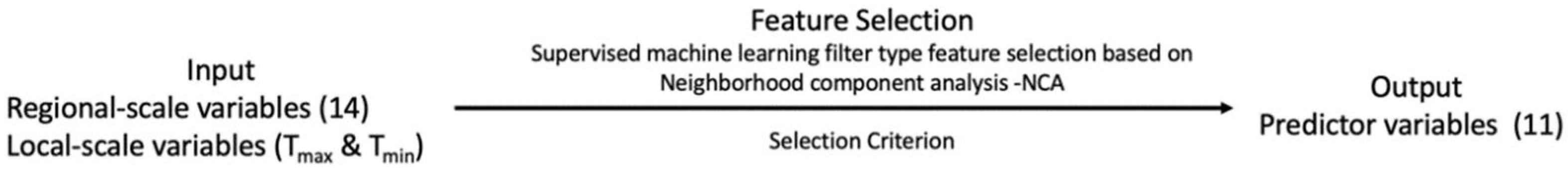
3.2. Feature Selection

The optimal predictor subset of climatic variables was determined using the NCA-based feature selection method, which assigns weights for each of the possible input variables (after standardization). The relative percentage weights for Tmax and Tmin are presented in Table 4 for the initial subset of 14 climatic variables.
The number of input variables was reduced based on two criteria: (a) the weights of the selected variables that had the largest relative contribution, and (b) they represented 85% of the total weight. The 11 final selected variables were common for both Tmax and Tmin, even though they exhibit different relative contributions (i.e., weights), and are shown in bold in Table 4.

3.3. Evaluation of Machine Learning Model Performance

The trained machine learning models that link the regional and local scales for each grid cell of the study area were applied for evaluation of the available data during 2012. More specifically, the values of the RCM variables were inserted in the models as predictors, and the obtained Tmax and Tmin results were compared with the corresponding UrbClim model simulations. This process was performed separately for each RCM model and each method (i.e., ANN and MLR).
The average annual results are presented in Figure 4, Figure 5, Figure 6 and Figure 7. Moreover, for a better comparison of the final (local) and initial (regional) scale, the temperature data of the regional models are also presented. It should be noted that for better visualization of the results, the temperature scale is the same for Tmax and Tmin.
Table 5, Table 6 and Table 7 below exhibit the average seasonal and annual MAE and BIAS statistical metrics, along with the R between the downscaling results and the UrbClim model simulations for both Tmax and Tmin and methods during 2012. The BIAS metric was calculated by subtracting the UrbClim values from the downscaling results; hence, positive values of BIAS exhibited overestimation of the temperature from the downscaling procedure. It should be also noted that the statistical errors were first calculated for each day and, subsequently, aggregated to their seasonal and annual values.
Table 5 shows that both methods exhibited similar results and that the MLR model was associated with slightly lower MAEs compared to the ANN in all cases. In general, the RACMO22E RCM exhibited lower MAEs than the ALADIN63 RCM and Tmin had lower MAEs compared to Tmax, except for in the winter. Regarding the seasonality of MAEs, the method exhibited a higher predictive ability during the summer (1.58 °C on average) and autumn (1.72 °C on average), indicating that the approach is very useful for the study of the urban thermal environment during the summer period when most of the heatwaves occur. The average MAE was 1.75 °C, which is sufficient for city-scale applications. It is worth noting that the values of MAE in each method and RCM were lower for Tmin in the spring, summer, and autumn, whereas this was reversed in the winter where the lower values corresponded to Tmax.
Regarding the overall BIAS error results, Tmax was found to have a negative BIAS in contrast with Tmin, which had mainly a positive BIAS. When focusing on seasonal BIAS, the ALADIN63 model had the lowest BIAS errors when the MLR method was applied from the spring to autumn, compared to the ANN method which had a lower BIAS in the winter. For the RACMO22E model, the BIAS errors for Tmin in the spring were lower with the ANN method; however, for the rest of the seasons, no specific pattern was evident, neither for the ANN nor MLR methods.
The correlation analysis results indicated that a strong correlation exists in all cases, especially for the RACMO22E RCM. Regarding the correlation coefficient of Tmax, higher values were found for the MLR method when the ALADIN63 RCM was used, contrary to the RACMO22E RCM which exhibited the same high values of R regardless of the applied methodology.
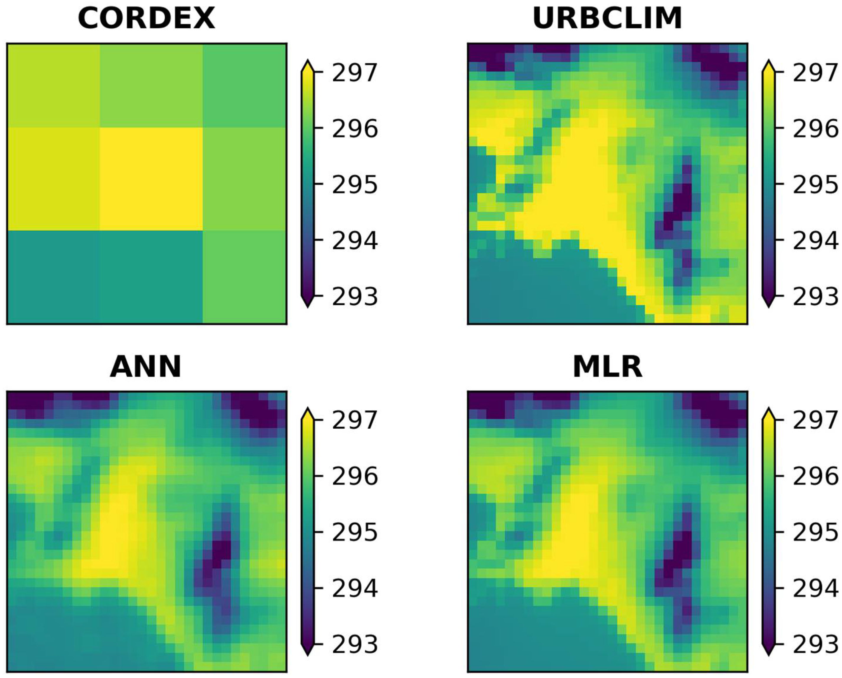
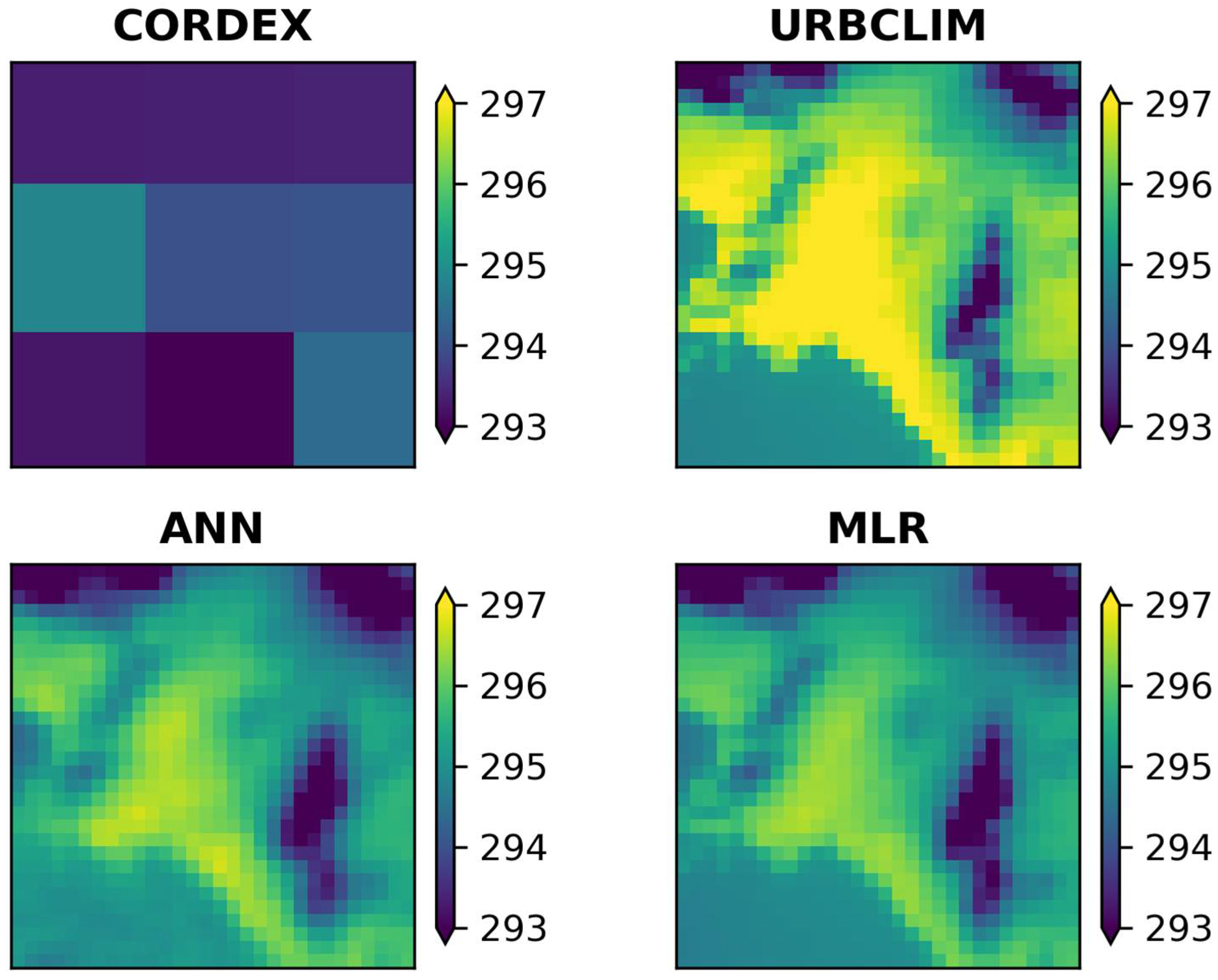
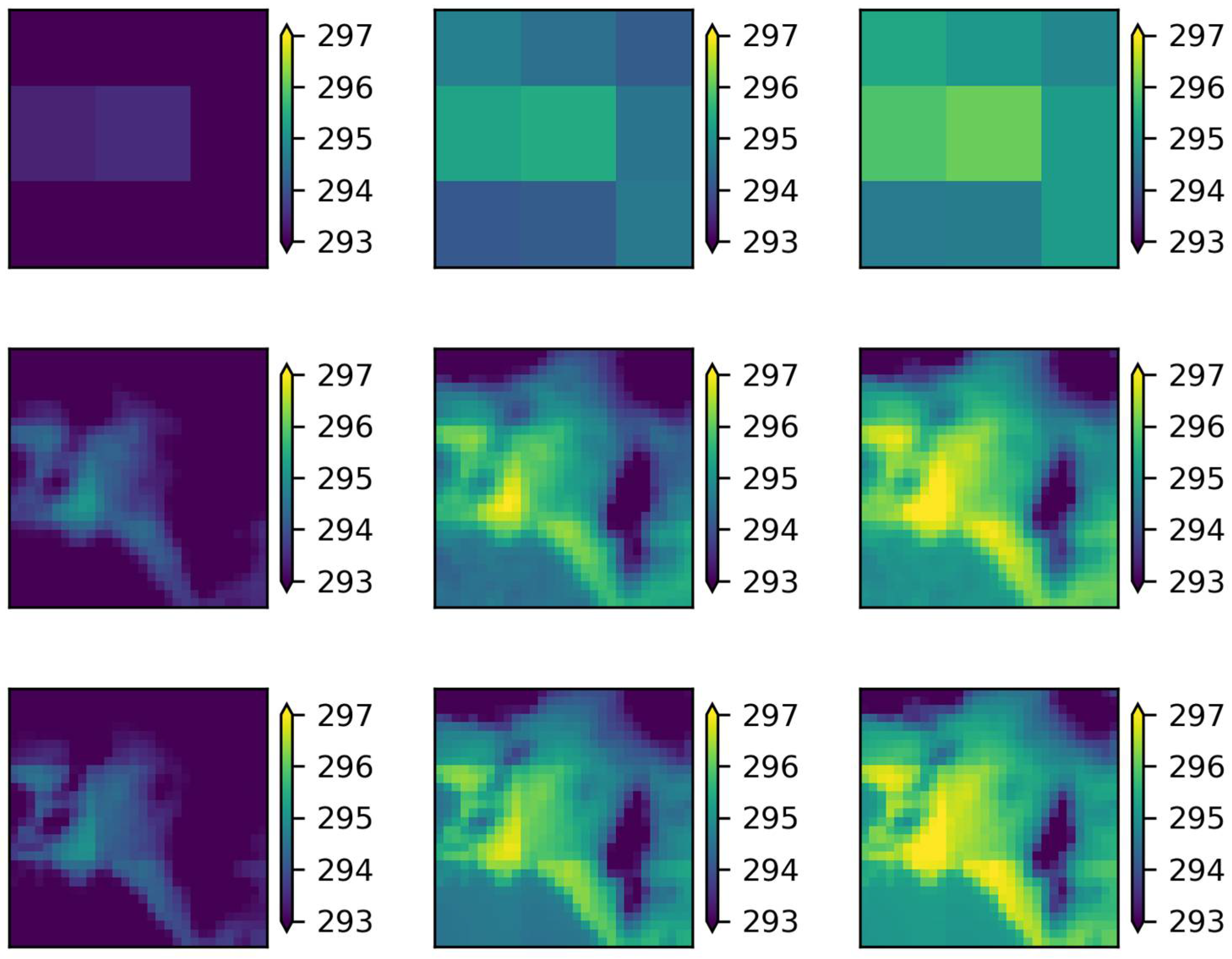
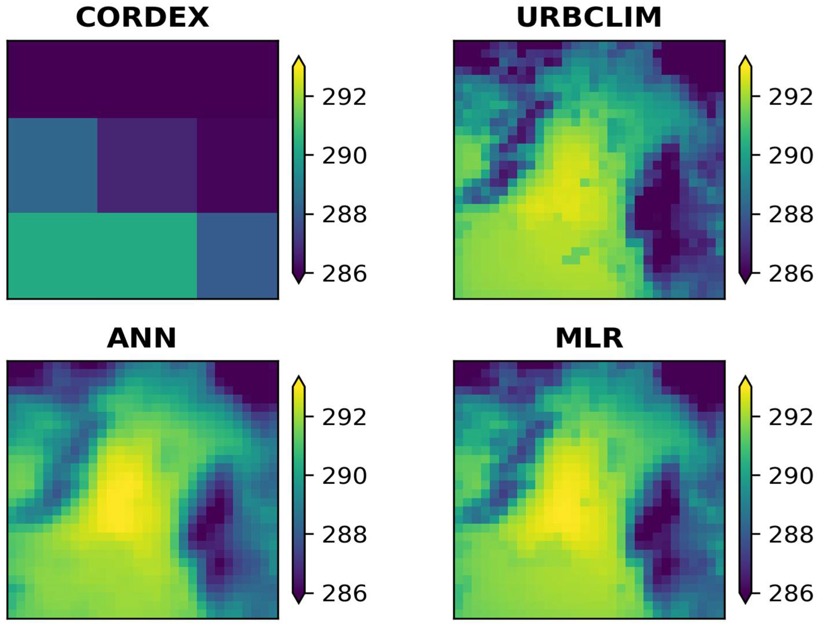
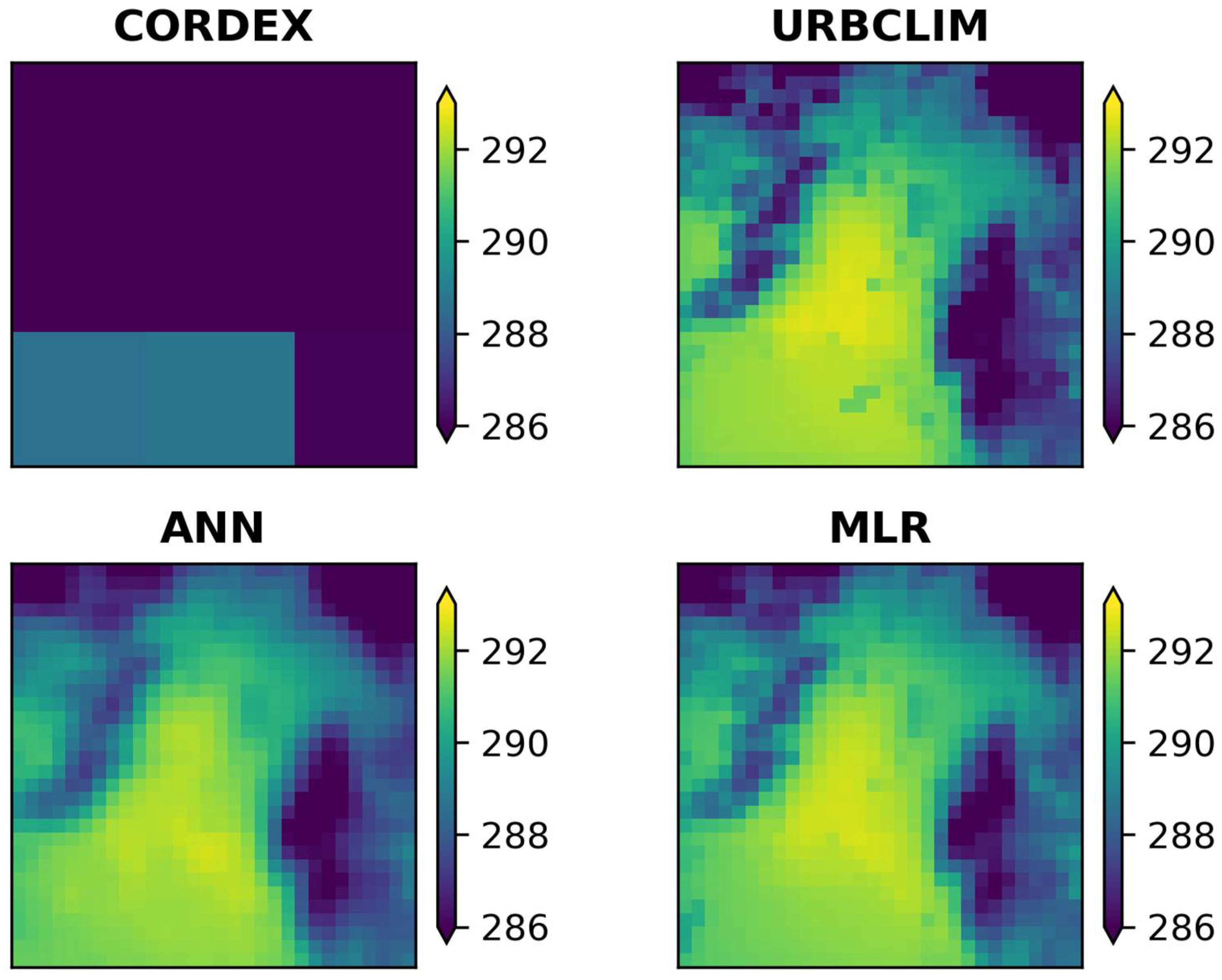
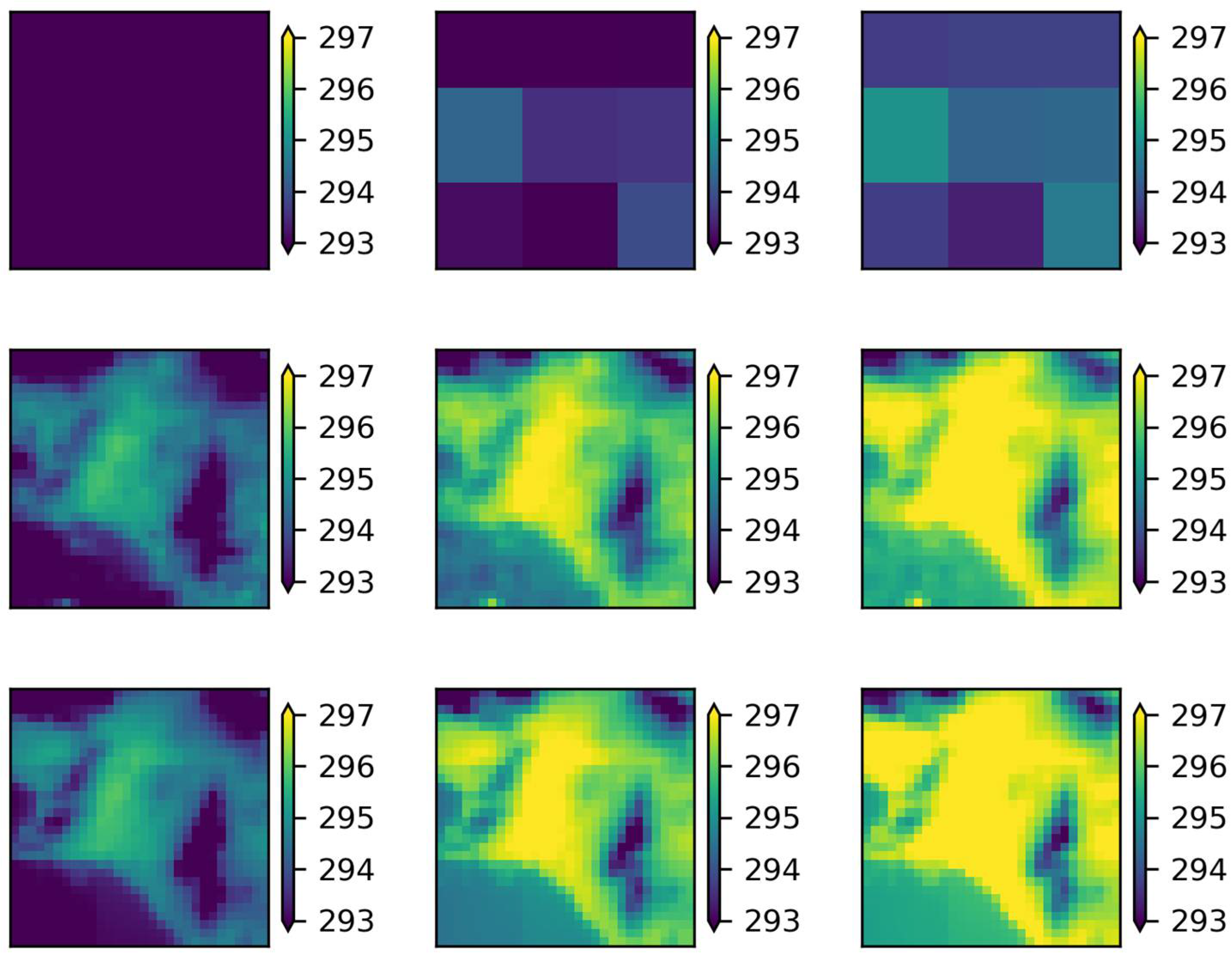
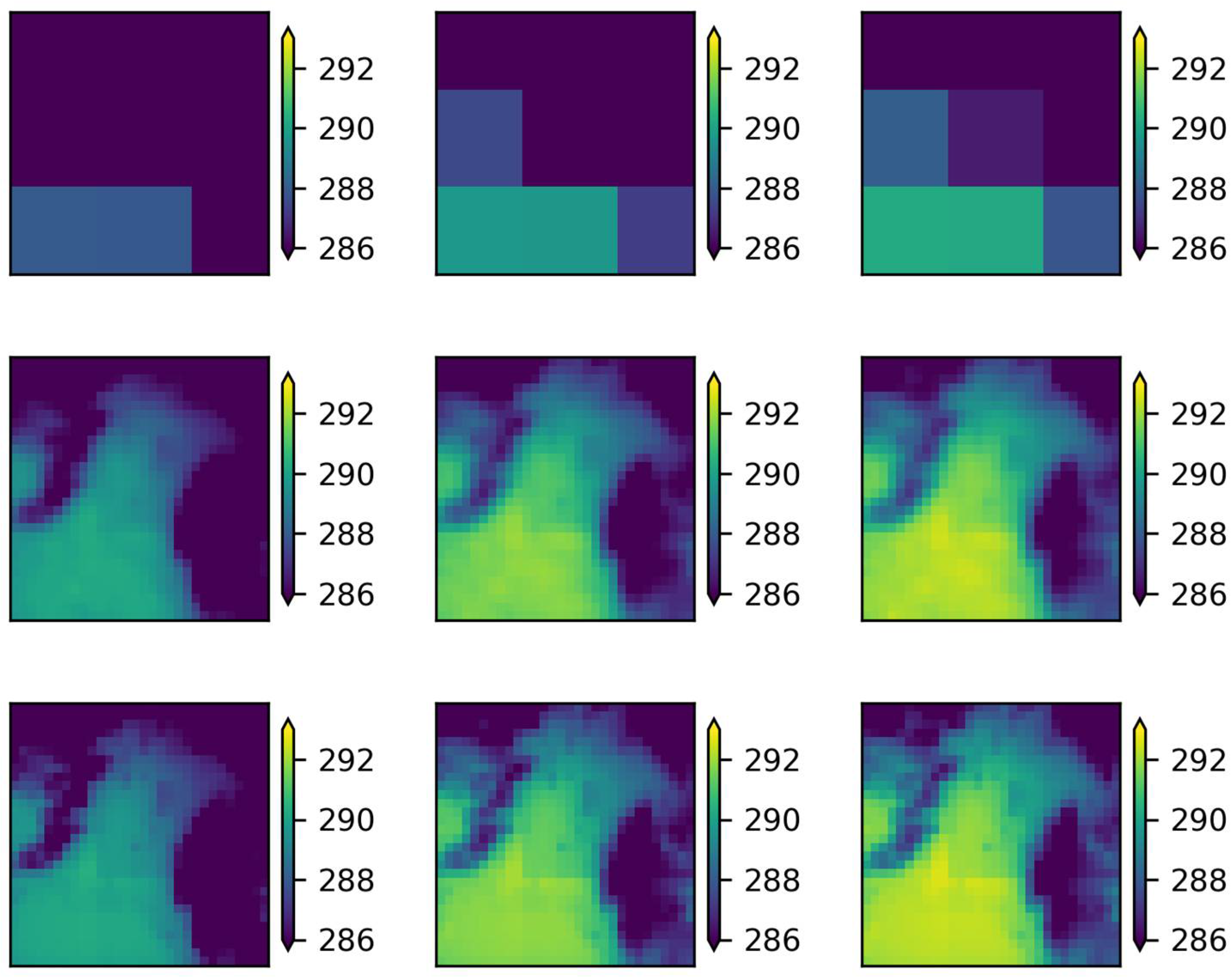
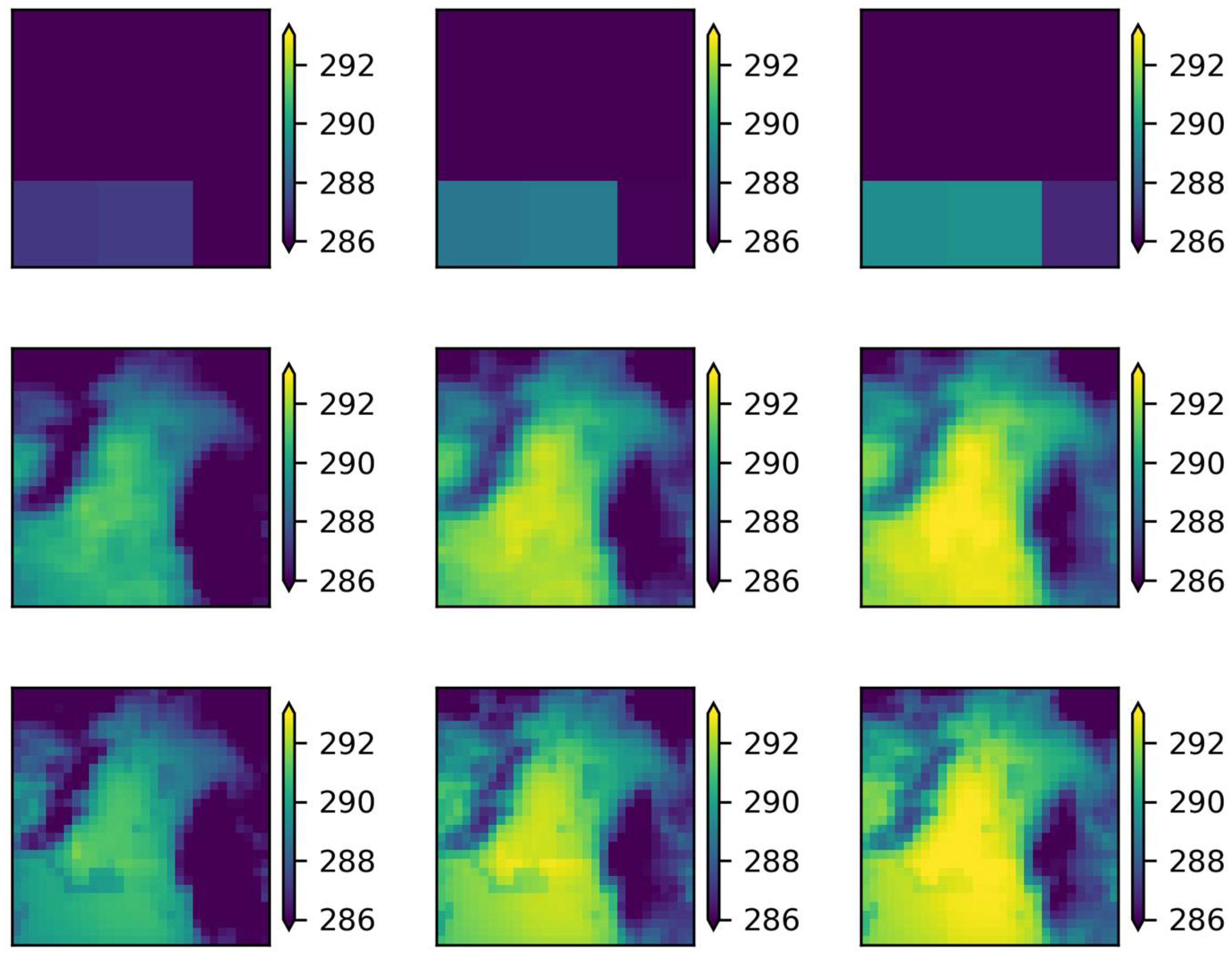
Analyzing the corresponding maps in Figure 4, Figure 5, Figure 6 and Figure 7, it was observed that both RCMs and the two methods successfully simulated the spatial patterns of temperature for the study area as they highlight the differences between the mountainous and urban areas, which were not distinguished at the regional scale, and approach, to a large extent, the scale of the UrbClim model (e.g., intra-urban temperature differences). Focusing on the annual average spatial Tmax distribution (Figure 4 and Figure 5), it was clearly observed that for both methods the mountainous and warmer urban areas of the western suburbs were accurately identified. Concerning the Tmin results, for the ALADIN63 model (Figure 6), the urban and mountainous areas’ temperature differences were well-identified; however, there was an underestimation of the Tmin in the western part of the domain and an overestimation in its central area for both methods. The same applies in the case of the RACMO22E model (Figure 7).
In conclusion, the relationships extracted from the ANN and MLR methods for the statistical downscaling of Tmax and Tmin to 1 km provided satisfactory results. This conclusion emerges both from the evaluation of the statistical analysis, since the R ranged from 0.93–0.97 and the MAE from 1.39–2.10 °C, as well as from the interpretation of the spatial temperature patterns over the domain under study.

3.4. Application of the Models at Historical and Future Periods

The ensemble of each grid-cell-trained ANN and MLR models were applied both in the historical 1971–2000 and in the future 2041–2070 periods. The application in the future period was applied for two different scenarios: the moderate RCP4.5 and the adverse RCP8.5. In addition, the methodology was applied separately for each RCM, initially for Tmax and subsequently for Tmin. The RCM results and projections of the 11 selected variables (predictors) were used to generate daily high-resolution maps of both Tmax and Tmin for the study area. Average monthly, seasonal, and 30-year climatological period maps were generated and compared in terms of the effect of climate change on the spatiotemporal distribution of Tmax and Tmin in high resolution over the study area. In Figure 8, Figure 9, Figure 10 and Figure 11, the average 30-year climatological period maps are presented for Tmax and Tmin of both RCMs upon the application of the ANN and the MLR downscaling methods. In Table 8 and Table 9, the results of the seasonal temperature differences between the reference historical and future periods for the two RCP scenarios are presented for both the ANN and the MLR methods.
Regarding Tmax, similar increases were identified for both models per scenario. More specifically, in the ALADIN63 model, both methods estimated that the largest increase will be observed during the summer season (approximately 2.2 °C for RCP4.5 and 2.5 °C for RCP8.5), and the smallest during the winter (approximately 1.5 °C and 2.1 °C for RCP4.5 and RCP8.5, respectively). Furthermore, the increased differences between the two scenarios for Tmax were estimated to be lower during the summer compared to the other seasons. Regarding the transitional periods, a stronger thermal signal was identified upon the application of both downscaling methods during the autumn as compared to spring for both RCMs under both RCPs. Looking at the RACMO22E model in more detail, the temperature increase was found to be approximately 1.8 °C for RCP4.5 and 2.55 °C for RCP8.5 for the ANN downscaling method during the autumn. An overall agreement was found for the spring, when the lowest Tmax increases were identified (1.3 °C for the moderate scenario and 2 °C for the adverse).
Regarding the seasonal variation of the average Tmin, the increase identified by each method was also very similar. For the ALADIN63 model, it was observed that the results obtained from the MLR method were about 0.15 °C higher than those from the ANNs. Furthermore, both methods in both scenarios predicted a larger increase in the summer of approximately 1.9 °C and 2.3 °C for RCP4.5 and RCP8.5. The smallest increase was predicted for the winter period, about 1.2 °C and 1.7 °C for the moderate and adverse scenarios, respectively. In the RACMO22E model, the results of the two methods were almost identical. In any case, the largest increase corresponded to summer and the smallest to spring. In the RCP4.5 scenario, the increase in the summer was about 1.9 °C and in the spring 1.1 °C, whereas in RCP8.5 it was 2.4 °C and 2 °C, respectively.
Furthermore, the results showed that, in general, the increase in the average Tmin is predicted to be smaller compared to Tmax. The only case this is reversed is in the summer period for the RACMO22E model, for the ANN method in both scenarios, and, also, in the spring for the RCP8.5 scenario.

4. Discussion and Conclusions

The present study focused on the statistical downscaling of two RCMs using two different methods, ANN and MLR. The aim was to identify the relationships between the regional and the local scale in order to improve the climate projections of the daily Tmax and Tmin in urban areas.
The developed models achieved a significant improvement for both the Tmax and Tmin projections compared to those of the initial RCMs and closely approached the local-scale spatiotemporal patterns of the UrbClim model simulations (e.g., the influence of the urban and the mountainous areas in Tmax and Tmin that could not be distinguished in the RCM simulations, but which stand out after downscaling the projections at 1 km).
In general, by comparing the two methods, it was observed that both the ANN and MLR performed reasonably well and were able to adequately reproduce both the Tmax and Tmin. The errors indicated that the two methods exhibited slight differences in accuracy. The MLR method had lower MAE values, whereas the ANN was associated with systematically lower BIAS. Considering the Tmax and Tmin spatial distribution, it was observed that the MLR had more uniform temperature fields, and the influence of the RCMs seemed to be greater. On the other hand, this effect was eliminated in the ANN.
Regarding the evaluation results of the dynamical-statistical downscaling method (simulations for 2012), it was observed that the Tmin was better approximated by both methods in the spring, summer, and autumn, whereas the opposite was observed for the winter season. Moreover, the values of the statistical metrics and the differences in their spatial distributions when compared to the UrbClim simulations (i.e., map comparison), showed that the best results were found during the summer, followed by spring and autumn.
In addition, the application of the models for the reference historical and future periods showed that, even though each RCM temperature projections differed, the differences that arose between the two time periods converged to almost the same values. This agrees with the fact that RCMs are more capable of predicting temperature change in the future than their absolute value. The change in the average Tmax and Tmin between the two methods was similar, and larger increases were observed for Tmax and Tmin during the summer.
In agreement with previous studies, this study concludes that there is no one single satisfactory solution for downscaling Tmax and Tmin, since both the ANN and the MLR methods had both advantages and disadvantages. In the present study, the two methods were used to establish transfer functions with different levels of complexity between the associated scales. An inherent advantage of using ANN models is their ability to model nonlinear relationships, whereas the MLR models can be used upon training to establish linear transfer functions. A drawback of using the ANN in the context of downscaling climate information in the urban environment is the requirement of a representative long-term training dataset. On the other hand, MLR methods follow a simpler training procedure that could provide sufficient results with significantly lower demands in terms of training. Upon availability, both approaches can be further enhanced through the use of auxiliary variables such as urban morphological characteristics. ANNs compared to MLR models can be used more efficiently to model extreme values through optimizing the training process and solving the overfitting issue effectively. Therefore, the appropriate choice of the downscaling method is related to both the complexity of the relationship between the two scales and the availability of high-resolution urban climate information. However, it should be noted that in the case of scarce data availability, the approach of a fully dynamical downscaling process through cascade modeling could be the optimum solution for urban impact studies. The choice of the appropriate method should be investigated each time and should be based on the spatial and temporal requirements of each study.
In a future study, the selection of different predictor variables for each method and/or each regional model could be investigated. An upper-atmospheric predictor could be used, such as the thickness layer between 1000–500 hPa or the 500 hPa geopotential in order to provide the models with more information from the general atmospheric circulation. In addition, an ensemble of regional climate models could also be used which would improve the accuracy of the estimates and reduce uncertainty. Moreover, the number of downscaling methods could be increased by applying, for example, the delta method or weather type classification. The overall framework could be applied to an even finer spatial resolution and simulations with the atmospheric WRF (Weather Research and Forecasting) model could be performed to generate and use high spatial resolution data in urban areas.
The urban climate depends on urban morphology parameters such as land cover and building height, among others, which are not directly considered in this study but have a direct influence on the meteorological parameters that were used for the downscaling techniques. To this end, the results of this work are useful for the assessment of the intra-urban spatial and temporal variability of the urban thermal environment and, therefore, could contribute to the identification of specific areas where adaptation plans should be prioritized.
In addition, the results are valuable for addressing urban climate change, and provide a methodology for practically assessing the state of the urban thermal environment at a finer scale in future climate scenarios. Accordingly, they serve as scientific evidence with respect to the strong need for the strengthening of the adaptive capacity and resilience of cities to climate change.

Author Contributions

All authors designed the methodology. K.K.-K. implemented the methodology and performed the statistical analysis; all authors contributed to the analysis of the data, interpretation of the results, and the writing of the paper. All authors have read and agreed to the published version of the manuscript.

Funding

This research was funded by the project “National Network for Climate Change and its Impacts–CLIMPACT”, which is implemented under the action “National Research Networks Infrastructures in the Fields of Medical Precision, Quantum Technologies and Climate Change” (code no. 2018ΣΕ01300001) financed by the Public Investments Program of Greece.

Data Availability Statement

The EURO-CORDEX datasets are available from Centre for Environmental Data Analysis (CEDA) (https://esgf-index1.ceda.ac.uk/search/esgf-ceda/ (accessed on 3 April 2022)). The UrbClim simulations were accessed from the Copernicus Climate Change Service (https://cds.climate.copernicus.eu/cdsapp#!/dataset/sis-urban-climate-cities?tab=overview (accessed on 3 April 2022)). The meteorological time series were accessed from the National Observatory of Athens (https://meteosearch.meteo.gr/ (accessed on 3 April 2022)).

Conflicts of Interest

The authors declare no conflict of interest.

References

  1. Masson-Delmotte, V.; Zhai, P.; Pörtner, H.-O.; Roberts, D.; Skea, J.; Shukla, P.R.; Pirani, A.; Moufouma-Okia, W.; Péan, C.; Pidcock, R.; et al. Global Warming of 1.5 °C—An IPCC Special Report on the Impacts of Global Warming of 1.5 °C; Intergovernmental Panel on Climate Change (IPCC): Geneva, Switzerland, 2018; Volume 1. [Google Scholar]
  2. Coumou, D.; Rahmstorf, S. A Decade of Weather Extremes. Nat. Clim. Chang. 2012, 2, 491–496. [Google Scholar] [CrossRef]
  3. Fischer, E.M.; Beyerle, U.; Knutti, R. Robust Spatially Aggregated Projections of Climate Extremes. Nat. Clim. Chang. 2013, 3, 1033–1038. [Google Scholar] [CrossRef]
  4. Mueller, B.; Zhang, X.; Zwiers, F.W. Historically Hottest Summers Projected to Be the Norm for More than Half of the World’s Population within 20 Years. Environ. Res. Lett. 2016, 11, 044011. [Google Scholar] [CrossRef]
  5. Fischer, E.M.; Sippel, S.; Knutti, R. Increasing Probability of Record-Shattering Climate Extremes. Nat. Clim. Chang. 2021, 11, 689–695. [Google Scholar] [CrossRef]
  6. Rosenzweig, C.; Solecki, W.D.; Hammer, S.A.; Mehrotra, S. Climate Change and Cities: First Assessment Report of the Urban Climate Change Research Network; Cambridge University Press: Cambridge, UK, 2011. [Google Scholar]
  7. Rahmati, O.; Darabi, H.; Panahi, M.; Kalantari, Z.; Naghibi, S.A.; Ferreira, C.S.S.; Kornejady, A.; Karimidastenaei, Z.; Mohmadi, F.; Stefanidis, S.; et al. Development of novel hybridized models for urban flood susceptibility mapping. Sci. Rep. 2020, 10, 12937. [Google Scholar] [CrossRef]
  8. Paravantis, J.; Santamouris, M.; Cartalis, C.; Efthymiou, C.; Kontoulis, N. Mortality Associated with High Ambient Temperatures, Heatwaves, and the Urban Heat Island in Athens, Greece. Sustainability 2017, 9, 606. [Google Scholar] [CrossRef] [Green Version]
  9. Santamouris, M. On the energy impact of urban heat island and global warming on buildings. Energy Build. 2014, 82, 100–113. [Google Scholar] [CrossRef]
  10. Trzaska, S.; Schnarr, E. A Review of Downscaling Methods for Climate Change Projections; The United States Agency for International Development by Tetra Tech ARD: Los Angeles, CA, USA, 2014; p. 56. [Google Scholar]
  11. Ayar, P.V.; Vrac, M.; Bastin, S.; Carreau, J.; Déqué, M.; Gallardo, C. Intercomparison of Statistical and Dynamical Downscaling Models under the EURO-and MED-CORDEX Initiative Framework: Present Climate Evaluations. Clim. Dyn. 2016, 46, 1301–1329. [Google Scholar] [CrossRef] [Green Version]
  12. Torma, C.; Giorgi, F.; Coppola, E. Added Value of Regional Climate Modeling over Areas Characterized by Complex Terrain—Precipitation over the Alps. J. Geophys. Res. Atmos. 2015, 120, 3957–3972. [Google Scholar] [CrossRef]
  13. Jacob, D.; Teichmann, C.; Sobolowski, S.; Katragkou, E.; Anders, I.; Belda, M.; Benestad, R.; Boberg, F.; Buonomo, E.; Cardoso, R.M.; et al. Regional Climate Downscaling over Europe: Perspectives from the EURO-CORDEX Community. Reg. Environ. Chang. 2020, 20, 51. [Google Scholar] [CrossRef]
  14. McSHEA, W.J. What Are the Roles of Species Distribution Models in Conservation Planning? Environ. Conserv. 2014, 41, 93–96. [Google Scholar] [CrossRef] [Green Version]
  15. Senay, S.D.; Worner, S.P. Multi-Scenario Species Distribution Modeling. Insects 2019, 10, 65. [Google Scholar] [CrossRef] [PubMed] [Green Version]
  16. Lim, Y.-K.; Shin, D.W.; Cocke, S.; LaRow, T.E.; Schoof, J.T.; O’Brien, J.J.; Chassignet, E.P. Dynamically and Statistically Downscaled Seasonal Simulations of Maximum Surface Air Temperature over the Southeastern United States. J. Geophys. Res. Atmos. 2007, 112. [Google Scholar] [CrossRef] [Green Version]
  17. Le Roy, B.; Lemonsu, A.; Schoetter, R. A Statistical–Dynamical Downscaling Methodology for the Urban Heat Island Applied to the EURO-CORDEX Ensemble. Clim. Dyn. 2021, 56, 2487–2508. [Google Scholar] [CrossRef]
  18. Maraun, D.; Wetterhall, F.; Ireson, A.; Chandler, R.; Kendon, E.; Widmann, M.; Brienen, S.; Rust, H.; Sauter, J.; Themel, M.; et al. Precipitation Downscaling under Climate Change: Recent Developments to Bridge the Gap between Dynamical Models and the End User. Rev. Geophys. 2010, 48, RG3003. [Google Scholar] [CrossRef]
  19. Gutiérrez, J.M.; Maraun, D.; Widmann, M.; Huth, R.; Hertig, E.; Benestad, R.; Roessler, O.; Wibig, J.; Wilcke, R.; Kotlarski, S.; et al. An Intercomparison of a Large Ensemble of Statistical Downscaling Methods over Europe: Results from the VALUE Perfect Predictor Cross-Validation Experiment. Int. J. Climatol. 2019, 39, 3750–3785. [Google Scholar] [CrossRef]
  20. Fowler, H.J.; Blenkinsop, S.; Tebaldi, C. Linking Climate Change Modelling to Impacts Studies: Recent Advances in Downscaling Techniques for Hydrological Modelling. Int. J. Climatol. J. R. Meteorol. Soc. 2007, 27, 1547–1578. [Google Scholar] [CrossRef]
  21. Hertig, E.; Seubert, S.; Paxian, A.; Vogt, G.; Paeth, H.; Jacobeit, J. Statistical Modelling of Extreme Precipitation Indices for the Mediterranean Area under Future Climate Change. Int. J. Climatol. 2014, 34, 1132–1156. [Google Scholar] [CrossRef]
  22. Timbal, B.; Dufour, A.; McAvaney, B. An Estimate of Future Climate Change for Western France Using a Statistical Downscaling Technique. Clim. Dyn. 2003, 20, 807–823. [Google Scholar] [CrossRef]
  23. Piani, C.; Haerter, J.; Coppola, E. Statistical Bias Correction for Daily Precipitation in Regional Climate Models over Europe. Theor. Appl. Climatol. 2010, 99, 187–192. [Google Scholar] [CrossRef] [Green Version]
  24. Turco, M.; Llasat, M.C.; Herrera, S.; Gutiérrez, J.M. Bias Correction and Downscaling of Future RCM Precipitation Projections Using a MOS-Analog Technique. J. Geophys. Res. Atmos. 2017, 122, 2631–2648. [Google Scholar] [CrossRef] [Green Version]
  25. Wilby, R.L.; Charles, S.P.; Zorita, E.; Timbal, B.; Whetton, P.; Mearns, L.O. Guidelines for Use of Climate Scenarios Developed from Statistical Downscaling Methods; Intergovernmental Panel on Climate Change (IPCC): Geneva, Switzerland, 2004; Volume 27. [Google Scholar]
  26. Eden, J.M.; Widmann, M. Downscaling of GCM-Simulated Precipitation Using Model Output Statistics. J. Clim. 2014, 27, 312–324. [Google Scholar] [CrossRef]
  27. Maraun, D.; Widmann, M. Structure of Statistical Downscaling Methods. In Statistical Downscaling and Bias Correction for Climate Research; Cambridge University Press: Cambridge, UK, 2018; pp. 135–140. [Google Scholar]
  28. Eden, J.M.; Widmann, M.; Grawe, D.; Rast, S. Skill, Correction, and Downscaling of GCM-Simulated Precipitation. J. Clim. 2012, 25, 3970–3984. [Google Scholar] [CrossRef] [Green Version]
  29. Careto, J.A.M.; Soares, P.M.M.; Cardoso, R.M.; Herrera, S.; Gutiérrez, J.M. Added Value of EURO-CORDEX High-Resolution Downscaling over the Iberian Peninsula Revisited—Part 2: Max and Min Temperature. Geosci. Model Dev. 2022, 15, 2653–2671. [Google Scholar] [CrossRef]
  30. Langendijk, G.S.; Rechid, D.; Jacob, D. Urban Areas and Urban–Rural Contrasts under Climate Change: What Does the EURO-CORDEX Ensemble Tell Us?—Investigating near Surface Humidity in Berlin and Its Surroundings. Atmosphere 2019, 10, 730. [Google Scholar] [CrossRef] [Green Version]
  31. Hamdi, R.; Van de Vyver, H.; De Troch, R.; Termonia, P. Assessment of Three Dynamical Urban Climate Downscaling Methods: Brussels’s Future Urban Heat Island under an A1B Emission Scenario. Int. J. Climatol. 2014, 34, 978–999. [Google Scholar] [CrossRef]
  32. DuchÊne, F.; Schaeybroeck, B.V.; Caluwaerts, S.; Troch, R.D.; Hamdi, R.; Termonia, P. A Statistical—Dynamical Methodology to Downscale Regional Climate Projections to Urban Scale. J. Appl. Meteorol. Climatol. 2020, 59, 1109–1123. [Google Scholar] [CrossRef]
  33. Hoffmann, P.; Krueger, O.; Schlünzen, K.H. A Statistical Model for the Urban Heat Island and Its Application to a Climate Change Scenario. Int. J. Climatol. 2012, 32, 1238–1248. [Google Scholar] [CrossRef]
  34. Wilby, R.L. Constructing Climate Change Scenarios of Urban Heat Island Intensity and Air Quality. Environ. Plan. B Plan. Des. 2008, 35, 902–919. [Google Scholar] [CrossRef] [Green Version]
  35. Burgstall, A.; Kotlarski, S.; Casanueva, A.; Hertig, E.; Fischer, E.; Knutti, R. Urban Multi-Model Climate Projections of Intense Heat in Switzerland. Clim. Serv. 2021, 22, 100228. [Google Scholar] [CrossRef]
  36. Rajczak, J.; Kotlarski, S.; Salzmann, N.; Schär, C. Robust Climate Scenarios for Sites with Sparse Observations: A Two-Step Bias Correction Approach. Int. J. Climatol. 2016, 36, 1226–1243. [Google Scholar] [CrossRef] [Green Version]
  37. Shin, Y.; Yi, C. Statistical Downscaling of Urban-Scale Air Temperatures Using an Analog Model Output Statistics Technique. Atmosphere 2019, 10, 427. [Google Scholar] [CrossRef] [Green Version]
  38. van der Schriek, T.; Varotsos, K.V.; Giannakopoulos, C.; Founda, D. Projected Future Temporal Trends of Two Different Urban Heat Islands in Athens (Greece) under Three Climate Change Scenarios: A Statistical Approach. Atmosphere 2020, 11, 637. [Google Scholar] [CrossRef]
  39. Früh, B.; Becker, P.; Deutschländer, T.; Hessel, J.-D.; Kossmann, M.; Mieskes, I.; Namyslo, J.; Roos, M.; Sievers, U.; Steigerwald, T.; et al. Estimation of Climate-Change Impacts on the Urban Heat Load Using an Urban Climate Model and Regional Climate Projections. J. Appl. Meteorol. Climatol. 2011, 50, 167–184. [Google Scholar] [CrossRef]
  40. Hoffmann, P.; Schoetter, R.; Schlünzen, K.H. Statistical-Dynamical Downscaling of the Urban Heat Island in Hamburg, Germany. Meteorol. Z. 2018, 27, 89–109. [Google Scholar] [CrossRef]
  41. Schoetter, R.; Hidalgo, J.; Jougla, R.; Masson, V.; Rega, M.; Pergaud, J. A Statistical–Dynamical Downscaling for the Urban Heat Island and Building Energy Consumption—Analysis of Its Uncertainties. J. Appl. Meteorol. Climatol. 2020, 59, 859–883. [Google Scholar] [CrossRef] [Green Version]
  42. Walton, D.B.; Sun, F.; Hall, A.; Capps, S. A Hybrid Dynamical–Statistical Downscaling Technique. Part I: Development and Validation of the Technique. J. Clim. 2015, 28, 4597–4617. [Google Scholar] [CrossRef]
  43. De Ridder, K.; Lauwaet, D.; Maiheu, B. UrbClim—A Fast Urban Boundary Layer Climate Model. Urban Clim. 2015, 12, 21–48. [Google Scholar] [CrossRef] [Green Version]
  44. Kourtidis, K.; Georgoulias, A.K.; Rapsomanikis, S.; Amiridis, V.; Keramitsoglou, I.; Hooyberghs, H.; Maiheu, B.; Melas, D. A Study of the Hourly Variability of the Urban Heat Island Effect in the Greater Athens Area during Summer. Sci. Total Environ. 2015, 517, 162–177. [Google Scholar] [CrossRef] [Green Version]
  45. Lagouvardos, K.; Kotroni, V.; Bezes, A.; Koletsis, I.; Kopania, T.; Lykoudis, S.; Mazarakis, N.; Papagiannaki, K.; Vougioukas, S. The Automatic Weather Stations NOANN Network of the National Observatory of Athens: Operation and Database. Geosci. Data J. 2017, 4, 4–16. [Google Scholar] [CrossRef]
Figure 1. Study area and locations of the meteorological stations.
Climate 10 00106 g001
Figure 2. Methodology (a) and data stream flow (b).
Climate 10 00106 g002
Figure 3. Feature selection methodology.
Climate 10 00106 g003
Figure 4. Annual average Tmax (in K) during 2012 for ALADIN63 RCM (up left), UrbClim model (up right), ANN (bottom left), and MLR (bottom right) downscaling of the ALADIN63 simulations.
Climate 10 00106 g004
Figure 5. Annual average Tmax (in K) during 2012 for RACMO22E RCM (up left), UrbClim model (up right), ANN (bottom left), and MLR (bottom right) downscaling of the RACMO22E simulations.
Climate 10 00106 g005
Figure 6. Annual average Tmin (in K) during 2012 for ALADIN63 RCM (up left), UrbClim model (up right), ANN (bottom left), and MLR (bottom right) downscaling of the ALADIN63 simulations.
Climate 10 00106 g006
Figure 7. Annual average Tmin (in K) during 2012 for RACMO22E RCM (up left), UrbClim model (up right), ANN (bottom left), and MLR (bottom right) downscaling of the RACMO22E simulations.
Climate 10 00106 g007
Figure 8. Average Tmax (in K) of the historical period (1st column) and of the two future climate scenarios, RCP4.5 (2nd column) and RCP8.5 (3rd column), as obtained by ALADIN63 RCM (first row), and by downscaling with the ANN (second row) and MLR (third row) methods.
Climate 10 00106 g008
Figure 9. Average Tmax (in K) of the historical period (first column) and of the two future climate scenarios, RCP4.5 (second column) and RCP8.5 (third column), as obtained by RACMO22E RCM (first row), and by downscaling with the ANN (second row) and MLR (third row) methods.
Climate 10 00106 g009
Figure 10. Average Tmin (in K) of the historical period (first column) and of the two future climate scenarios, RCP4.5 (second column) and RCP8.5 (third column), as obtained by ALADIN63 RCM (first row), and by downscaling with the ANN (second row) and MLR (third row) methods.
Climate 10 00106 g010
Figure 11. Average Tmin (in K) of the historical period (first column) and of the two future climate scenarios, RCP4.5 (second column) and RCP8.5 (third column), as obtained by RACMO22E RCM (first row), and by downscaling with the ANN (second row) and MLR (third row) methods.
Climate 10 00106 g011
Table 1. List of EURO-CORDEX RCM simulations and driving experiments for each studied period.
PeriodRCMsExperiment
Historical (1971–2000)ALADIN63, RACMO22ECNRM-CERFACS-CNRM-CM5
Evaluation (2008–2012)ALADIN63, RACMO22EECMWF-ERAINT
Future (2041–2070)ALADIN63, RACMO22ECNRM-CERFACS-CNRM-CM5
Table 2. Representative meteorological stations and characteristics.
Meteorological StationLand-Use TypeLatitude (°)Longitude (°)
1. AlimosCoastal37.917523.7107
2. KantzaLow-Density Urban37.979323.8656
3. KifissiaHigh percentage of vegetation38.066123.8200
4. Neos KosmosHigh-Density Urban37.959023.7325
5. PalliniLow-Density Urban37.997823.8928
6. PatisiaHigh-Density Urban38.022023.7298
7. FaliroCoastal37.929423.6930
8. PsychikoHigh percentage of vegetation38.017623.7806
Table 3. Statistical metrics (R, MAE, MARE, RMSE, and BIAS) between UrbClim-simulated and -observed Tmax and Tmin values from 2016 to 2017 for selected stations.
RΜAΕ (°C)MARERMSE (°C)BIAS (°C)
TmaxTminTmaxTminTmaxTminTmaxTminTmaxTmin
Neos Kosmos0.990.981.081.450.050.121.391.90−0.031.17
Patisia0.980.951.411.940.070.191.722.55−0.621.40
Alimos0.970.981.741.680.080.142.432.141.181.51
Faliro0.980.971.431.510.060.131.942.030.431.20
Kifissia0.990.980.921.620.050.161.191.970.27−1.38
Psychiko0.990.970.911.360.050.171.181.78−0.300.81
Kantza0.990.961.271.820.070.291.632.36−0.03−1.13
Pallini0.990.971.281.260.060.171.681.580.50−0.10
Table 4. Relative percentage weights of contribution corresponding to each input variable to predict Tmax and Tmin as derived from the feature selection procedure (the optimal subset of variables is denoted in bold).
Climatic VariableWeight for Tmax (%)Weight for Tmin (%)
Evaporation5.14%5.39%
Relative Humidity8.15%7.98%
Sea-level Pressure7.24%6.15%
Surface Pressure6.75%6.90%
Downwelling Longwave Radiation7.79%7.53%
Downwelling Shortwave Radiation5.13%3.72%
Surface Temperature7.03%6.90%
Upwelling Latent Heat Flux5.13%5.38%
Downwelling Latent Heat Flux6.51%7.13%
Upwelling Longwave Radiation6.66%6.72%
Upwelling Shortwave Radiation6.40%6.65%
Maximum Temperature9.62%8.49%
Minimum Temperature8.99%8.91%
Soil Moisture9.46%12.16%
Table 5. Average seasonal and annual MAE (°C) between the downscaling results and the UrbClim model simulations during 2012 for Tmax and Tmin for both methods (i.e., MLR and ANN), and RCMs (i.e., ALADIN63 and RACMO22E).
ALADIN63RACMO22E
TmaxTminTmaxTmin
ANNMLRANNMLRANNMLRANNMLR
Winter2.151.982.342.281.771.561.901.57
Spring2.031.741.821.602.061.851.531.55
Summer1.891.751.481.301.831.681.511.23
Autumn2.342.001.921.761.691.501.401.21
20122.101.871.891.731.841.651.581.39
Table 6. Average seasonal and annual BIAS (°C) between the downscaling results and the UrbClim model simulations during 2012 for Tmax and Tmin for both methods (i.e., MLR and ANN) and RCMs (i.e., ALADIN63 and RACMO22E).
ALADIN63RACMO22E
TmaxTminTmaxTmin
ANNMLRANNMLRANNMLRANNMLR
Winter−0.35−0.660.770.61−0.53−0.980.640.28
Spring0.570.501.351.22−0.46−0.300.400.84
Summer−0.81−0.67−0.01−0.02−0.74−0.92−0.61−0.09
Autumn−0.37−0.220.170.11−0.91−0.93−0.63−0.17
2012−0.24−0.260.570.48−0.66−0.78−0.050.22
Table 7. Average seasonal and annual R between the downscaling results and the UrbClim model simulations during 2012 for Tmax and Tmin for both methods (i.e., MLR and ANN) and RCMs (i.e., ALADIN63 and RACMO22E).
ALADIN63RACMO22E
TmaxTminTmaxTmin
ANNMLRANNMLRANNMLRANNMLR
Winter0.700.720.660.520.880.880.760.82
Spring0.820.900.910.920.900.900.920.93
Summer0.710.760.740.820.760.770.730.85
Autumn0.750.860.740.760.940.940.880.89
20120.930.960.940.950.970.970.960.97
Table 8. Seasonal temperature differences for Tmax (°C) between the historical and future periods for both models and scenarios for the ANN and the MLR methods.
RCP4.5RCP8.5
ALADIN63RACMO22EALADIN63RACMO22E
ANNMLRANNMLRANNMLRANNMLR
Winter1.451.491.351.352.122.152.302.18
Spring1.561.601.221.342.402.381.822.15
Summer2.142.281.792.062.472.552.442.51
Autumn1.821.781.801.722.412.332.552.42
Table 9. Seasonal temperature differences for Tmin (°C) between the historical and future periods for both models and scenarios for the ANN and the MLR methods.
RCP4.5RCP8.5
ALADIN63RACMO22EALADIN63RACMO22E
ANNMLRANNMLRANNMLRANNMLR
Winter1.081.251.151.231.581.862.132.06
Spring1.211.321.091.231.912.071.882.05
Summer1.762.031.851.892.202.372.482.39
Autumn1.501.561.731.612.132.152.372.28
Publisher’s Note: MDPI stays neutral with regard to jurisdictional claims in published maps and institutional affiliations.

