Evaluation of Long-Term Trends of Rainfall in Perak, Malaysia

Abstract

This study aimed to examine the spatiotemporal seasonal and annual trends of rainfall indices in Perak, Malaysia, during the last 35 years, as any seasonal or spatial variability in rainfall may influence the regional hydrological cycle and water resources. Mann–Kendall and Sequential Mann–Kendall (SMK) tests were used to assess seasonal and annual trends. Precipitation concentration index was used to estimate variations in rainfall concentration, and Theil–Sen’s slope estimator was used to determine the spatial variability of rainfall. It was found that most of the rainfall indices are showing decreasing trends, and it was most prominent for the southwest monsoon season with a decreasing rate of 2.20 mm/year. The long-term trends for seasonal rainfall showed that rainfall declined by 0.29 mm/year during the southwest monsoon. In contrast, the northeast and the inter-monsoon seasons showed slight increases. Rainfall decreased gradually from 1994 to 2008, and the trend became more pronounced in 2008. On a spatial basis, rainfall trends have shifted from the western regions (i.e., −19 mm/year) to the southeastern regions (i.e., 10 mm/year). Overall, slightly decreasing trends in rainfall were observed in Perak Malaysia.

1. Introduction

Over the past few decades, greenhouse gas concentration has increased rapidly. The result of this increase has been global energy imbalance and global warming [1,2]. In its sixth assessment report, the Intergovernmental Panel on Climate Change (IPCC) predicted that global temperatures will rise by 1.5 °C by 2040 [3]. Climate change has been documented to play a key role in regulating the global as well as the regional hydrological cycle [4]. Rainfall is one of the major components of the hydrological cycle, and recent research indicates that a change in the global climate disrupts the natural rainfall cycle [5,6,7]. Rainfall provides the necessary understanding to quantify the intensity and severity of different hydrological phenomena, such as floods, droughts, and river discharge, etc. The estimation of seasonal and spatial trends of rainfall can provide valuable information not only to climatologists but also to weather forecasters, hydrologists, and decision-makers.

Previously, climate change research has been focused on detecting trends in hydroclimatic variables such as precipitation, evapotranspiration, and temperature [8]. An assessment of changes in the characteristics and patterns of these variables can provide a better understanding of how climate has changed over time. Since rainfall is highly stochastic in nature and because it varies on both a seasonal and spatial scale, there has been renewed interest in measuring rainfall trends to identify climate change [9]. In this regard, the working group of IPCC investigated the variations in spatiotemporal trends of rainfall from 1900 to 2005 over different regions of the world. Their results indicated a significant increase in rainfall over the central and northern regions of Asia [10]. Several studies have demonstrated a significant correlation between flooding and changes in the natural pattern of rainfall [11,12].

Flooding is regarded as the most destructive natural calamity in Malaysia. There are more than 29,000 km² exposed to flooding, which consequently affects approximately 4.82 million people with an estimated economic loss of USD 299 million [13,14]. Flooding in Malaysia is primarily caused by intense and frequent monsoons and convective rains [15]. Flooding in Pahang, Perak, and Kelantan between 20 December 2014, and 1 January 2015, has raised many uncertainties regarding future flooding risk. The predominant cause of this calamity, according to the Dartmouth Flood Observatory, was monsoon rainfall, which affected more than 215,000 people [16]. Therefore, owing to the stochastic and uncertain nature of rainfall, information about its spatial and temporal variability is essential for early flood warning and future planning.

In the recent past, several studies investigating trends and variability in hydroclimatic parameters have been conducted around the globe using different statistical methods [17,18,19,20]. Current research on rainfall analysis employs two basic statistical approaches; parametric and non-parametric tests. Both approaches have their advantages and disadvantages. Parametric tests suffer from a serious limitation, which is that they require normally distributed data for testing. However, hydro-climatic datasets rarely meet this requirement. As opposed to parametric tests, non-parametric tests are less sensitive to normally distributed data, and their ability to handle sudden breaks makes them more suitable for detecting trends in hydro-climatic variables. The Mann–Kendall (MK) test is a non-parametric test that has been used in many investigations into hydro-climatic trend analysis [7,21,22].

Peninsular Malaysia is situated in the tropical region and is located between 1° and 6° N on the northern latitude and 100° to 103° E on the eastern longitude. Due to its proximity to the equator, the country experiences humid and hot weather throughout the year, and the distribution of the rainfall is uneven. A study analysed the rainfall trends over Peninsular Malaysia on a seasonal and temporal basis using Spearman’s rank correlation test [23]. The entire region was divided into three distinct sections: the central, east, and west coasts. Study results showed significant increasing trends in annual precipitation over the west coast with significant spatial variability. Another study measured the intensity and concentration of daily rainfall on a spatial basis over Peninsular Malaysia in 2012 using an ordinary kriging approach. They also found a high irregularity in the distribution of diurnal rainfall over the eastern regions [24].

Research to date has centred mostly on the analysis of trends in Peninsular Malaysia. Quite a few studies, such as [25], investigated the long-term rainfall trends at the Langat River Basin, Selangor Malaysia, from 1980 to 2010 to explain the mechanisms behind spatially and temporally variable rainfall on a small scale. The study concluded the significant increasing trends in the annual rainfall and highlighted the need for the spatiotemporal trends detection in different rainfall indices on a comparatively small scale than entire Peninsular Malaysia. Perak is the fourth largest state in entire Malaysia, with an area of 21,035 km² and a population of 2.46 million. The past few decades have seen an increasing trend of flooding in the state [15]. Despite huge investments in flood management, the recurring nature of floods poses a serious threat to the state’s economy and the lives of its citizens. Some studies have concluded that increased rainfall trends on a spatiotemporal basis may contribute to frequent flooding [26].

However, the causes of intense flooding remain speculative. Therefore, to comprehend the underlying factors of frequent flooding, the assessment of spatial and temporal trends of rainfall can provide better insight. However, it appears that no study has been conducted for the assessment of spatiotemporal trends in rainfall over Perak, Malaysia. Consequently, the main objective of the study was to assess the spatiotemporal trends of rainfall in Perak, Malaysia. The specific objectives were (i) to examine the temporal variability and unexpected trend changes in rainfall indices; and (ii) to ascertain the spatial fluctuations in the seasonal and annual rainfall trends.

2. Study Area and Data Source

2.1. Description of the Study Area

Perak is located in the western region of Peninsular Malaysia covers an area of 21,035 km², which makes it the second-largest state in Peninsular Malaysia. Geographically, it is situated between the 100°0′ E to 102°0′ E latitude and 3°30′ N to 6°0′ N longitude (Figure 1). Agriculture is the major land use of the state that covers 41% area of the state followed by forest (28%), and urban lands encompass 22% area, respectively [27].

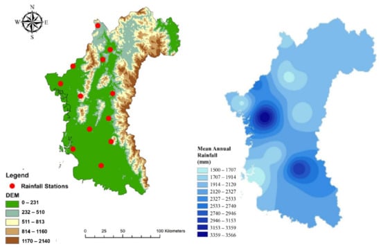
Figure 1. Characteristics of study area and distribution of mean annual rainfall over Perak, Malaysia.

The climate of the state can be described by four seasons; two monsoons, and two Inter-monsoon seasons. The first monsoon season, known as the Southwest monsoon (SWM), is comprised of four months from May to August. Whereas the second monsoon, i.e., the Northeast monsoon (NEM), spans from November to February. NEM brings high-intensity rainfall of 200–300 mm/season over the eastern parts of Peninsular Malaysia. However, the SWM is regarded as the drier season of Malaysia. In the case of inter-monsoonal seasons, they often receive intensive convective rainfalls [24].

2.2. Data Acquisition and Preliminary Analysis

Daily rainfall data from twelve (12) automatic rain gauges were acquired from the Department of Irrigation and Drainage, Malaysia, from 1980 to 2014. A plethora of factors was taken into account in choosing rainfall stations, including the availability of data, uniformity of data, environment, and other ancillary factors. The area-weighted daily rainfall for the Perak was prepared from the fixed network of the rain gauges and then monthly, seasonal, and annual rainfall values were extracted. In order to obtain uniform data, ArcGIS 10.3 was used to extrapolate precipitation using the ordinary kriging method. It is a geostatistical approach for measuring values at unsampled locations and is already used in various climatological and hydrological applications [28,29,30]. Moreover, due to the data constraints in the mountainous region, this research was unable to comprehend the full extent of rainfall coverage in the mountainous regions. Figure 1 provides the geographical location of all rainfall stations, whereas Table 1 presents the details of rainfall stations.

Table 1. Description of automatic rainfall stations with geographic coordinates in Perak, Malaysia (1980–2014).

Station ID	Location	Longitude	Latitude	Avg. Annual Rainfall
				(mm)
5710061	Dispensari Keroh	101.00	5.71	1881
5411066	Kuala Kenderong	101.15	5.42	1961
5210069	Stesen Pem. Hutan Lawin	101.06	5.30	1606
5207001	Kolam Air JKR Selama	100.70	5.22	2632
5005003	Jln. Mtg. Buloh Bgn Serai	100.55	5.01	1682
4811075	Rancangan Belia Perlop	101.18	4.89	1728
4807016	Bukit Larut Taiping	100.79	4.86	3566
4511111	Politeknik Ungku Umar	101.13	4.59	2178
4409091	Rumah Pam Kubang Haji	100.90	4.46	1730
4311001	Pejabat Daerah Kampar	101.16	4.31	3131
4207048	JPS Setiawan	100.70	4.22	1501
4010001	JPS Teluk Intan	101.04	4.02	2133

Table 2 presents the summary statistics of the monthly-, seasonal-, and annual rainfall over the state from 1980 to 2014. The average annual rainfall was observed as 2156 mm (SD = 337 mm) with a maximum of 2735 mm in 1999 and a minimum of 1353 mm in 2006. However, the relatively low value of the coefficient of variance (CV), i.e., 16%, indicated the low inter-annual variability of rainfall. On a monthly basis, November and October contribute the maximum share of annual rainfall by 13% and 12%, respectively, followed by April (10%) and September (9%). The least amount of rainfall falls in January (4%) and June (5%). Further analysis of CV for monthly values revealed the rainfall variability in February (45%), August (40%), and March (39%) were high compared with November (25%) and October (30%). It can be seen from Table 2 that inter-monsoon seasons receive the higher rainfall as inter-monsoon 2 (IM 2) shares 30% in the annual rainfall followed by inter-monsoon 1 (IM 1) by 26%. The contribution of NEM towards the annual rainfall share is 22%, followed by the SWM by 20%. Despite the small inter-annual variability in the annual rainfall, the NEM shows a comparably high value of CV (i.e., 48%), which implies the higher rainfall variations in seasonal rainfall over the years.

Table 2. Preliminary analysis of monthly, seasonal, and annual rainfall over Perak, Malaysia (1980–2014).

Months	Min.	Max.	SD.	Avg.	Coeff. of Var.	Share
	(mm)	(mm)	(mm)	(mm)	(%)	(%)
Jan	38.10	204.43	42.30	115.94	36	5.38
Feb	23.41	242.36	56.40	125.04	45	5.80
Mar	21.89	353.50	69.54	180.24	39	8.36
Apr	71.66	355.62	67.82	217.45	31	10.08
May	52.69	302.74	59.74	189.40	32	8.78
Jun	50.50	191.32	39.05	124.92	31	5.79
Jul	60.63	256.34	56.04	142.51	39	6.61
Aug	6.48	265.75	64.32	161.35	40	7.48
Sep	77.66	363.70	66.48	207.09	32	9.60
Oct	126.92	426.38	75.87	248.96	30	11.55
Nov	111.53	469.57	66.74	262.38	25	12.17
Dec	56.26	354.67	63.04	181.13	35	8.40
Annual	1352.93	2735.49	337.05	2156.41	16	100.00
NEM	23.41	469.57	81.86	171.12	48	22.74
IM 1	21.89	355.62	70.72	198.84	36	26.42
SWM	6.48	302.74	60.01	154.55	39	20.54
IM 2	77.66	426.38	73.88	228.03	32	30.30

3. Methodology

3.1. Rainfall Indices

This study utilized the rainfall indices for the detection of possible trends in daily rainfall. For assessing the impact of climate change on weather extremes, the Joint Technical Commission for Oceanography and Marine Meteorology (JCOMM) and Climate and Ocean-Variability, Predictability, and Change (CLIVAR) developed 27 indices using rainfall and temperature data on a daily basis. In this research, only the extreme indices that can be extracted from daily rainfall were chosen for the analysis. Altogether, ten indices were selected (Table 3). An R-environment program, RClimDexV3, developed by the Climate Research Branch of the Meteorological Service of Canada, was used to calculate the indices. This program was accessed from the ETCCDI’s website.

Table 3. Description of extreme rainfall indices.

Indices	Description	Units
RX1Day	Monthly maximum 1-day rainfall	mm
RX5Day	Monthly maximum consecutive 5-day rainfall	mm
R95p	Annual total rainfall when RR > 95p	mm
R99p	Annual total rainfall when RR > 99p	mm
PRCPTOT	Annual total rainfall in wet days	mm
R10mm	Annual count of days when Rainfall ≥ 10 mm	days
R20mm	Annual count of days when Rainfall ≥ 20 mm	days
CDD	Maximum length of dry spell, maximum number of consecutive days with RR < 1 mm	days
CWD	Maximum length of wet spell, maximum number of consecutive days with RR ≥ 1 mm	days
SDII	Simple precipitation intensity index	mm/day
NEM	Northeast Monsoon occurs from November to February	mm
IM 1	Inter-monsoon 1 occurs from March to April	mm
SWM	Southwest Monsoon occurs from May to August	mm
IM 2	Inter-monsoon 2 occurs from September to October	mm
Monthly	Monthly Rainfall	mm
Annual	Annual Rainfall	mm

Furthermore, before selecting the test to perform the trend analysis on the rainfall time series, it was proposed to confirm the normality of the data series. The Shapiro–Wilk (SW) test was used for this purpose. Based on the results of the SW test, Mann–Kendall (MK) test was chosen to identify monotonic trends in rainfall time series as it was evident that data sets were not normally distributed on a 95% confidence interval (Table 4). Sequential Mann–Kendall (SMK) test was used to identify abrupt changes in rainfall indices. The TSS estimator has been used to assess the spatial variability of rainfall at individual stations. A brief description of all methods is described in the following text.

Table 4. Results of Shapiro–Wilk test.

Indices	SW Test	p-Value
RX1Day	0.99	0.90
RX5Day	0.97	0.54
R95p	0.97	0.45
R99p	0.95	0.16
PRCPTOT	0.94	0.07
R10mm	0.93	0.03
R20mm	0.96	0.17
CDD	0.92	0.07
CWD	0.87	0.06
SDII	0.97	0.51
NEM	0.96	0.57
IM 1	0.99	0.63
SWM	0.99	0.31
IM 2	0.98	0.39
Monthly	0.98	0.10
Annual	0.94	0.07

Bold shows the significance.

3.2. Precipitation Concentration Index (PCI)

The Precipitation Concentration Index (PCI) was developed by Oliver (1980) [31] and has been used in various studies as the indicator for change in rainfall concentrations [32,33]. PCI was calculated at each station on an annual basis to analyse the trends and variability in the concentration of rainfall. It can be explained using Equation (1).

$$PC{I}_{annual}=\frac{{\sum }_{i=1}^{12} p_i^2}{{\left({\sum }_{i=1}^{12} p_i\right)}^2}\ast 100$$

(1)

Where p_i represents the monthly rainfall for the ith month, the minimum theoretical value of PCI is 8.3, demonstrating the uniform distribution of rainfall among all months [31]. However, the values of PCI larger than 16.7 indicate the irregular precipitation distribution and the values greater than 20 represent the strong irregular precipitation distribution.

3.3. Autocorrelation Analysis

Serial dependence is a major problem while testing the trends in time series. Application of any non-parametric tests on time series data without prior calculation of the serial dependence can result in significantly biased results. Therefore, before trend analysis, the lag-1 autocorrelation coefficient ($r_1$) was sought by using a two-tailed test. The calculation of $r_1$ was made by Equation (2).

$$r_1=\frac{\frac{1}{\left(n-1\right)}{\sum }_{i=1}^{n-1} \left(X_i-\overline{X}\right)\left(X_{i+1}-\overline{X}\right)}{{\sum }_{i=1}^n {\left(X_i-\overline{X}\right)}^2}$$

(2)

where X_i is the ith observation, $\stackrel{\_}{X}$ is the mean and n is the sample size. After testing the presence of$r_1$, the null hypothesis was tested on 0.05 significance using a two-tailed test by Equation (3).

$$r_1 \left(95\%\right)=\frac{-1\pm 1.96\sqrt{\left(n-2\right)}}{n-1}$$

(3)

It has been mentioned that if the value of $r_1$ is between the upper and lower bounds of the significance level, the time series is not serially correlated and the MK test can be applied directly to the time series [34]. The results obtained from the analysis of $r_1$ displayed a high correlation amongst the different rainfall indices’ datasets, e.g., PRCPTOT, R20mm, and IM 1 (Figure 2a,b). Therefore, the trend-free-pre-whitening (TFPW) approach was used to obtain the serially independent time series.

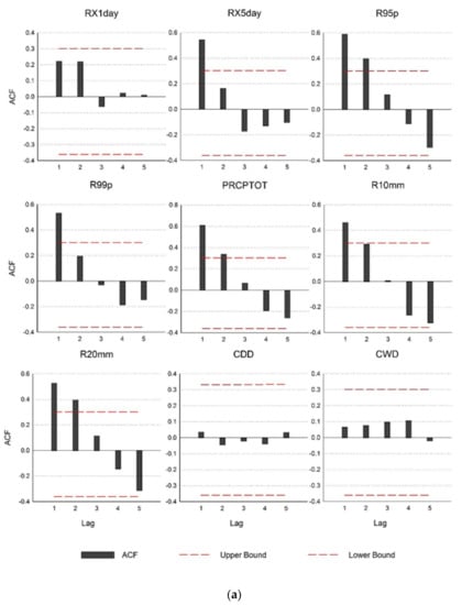
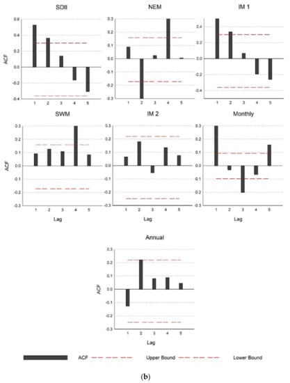
Figure 2. (a) Autocorrelation Function (ACF) analysis of rainfall indices. The red-dotted lines depict the 0.05 significance level and the x-axis shows the lag in the time series. (b) Autocorrelation Function (ACF) analysis of rainfall. The red dotted lines depict the 0.05 significance level, and the x-axis shows the lag in the time series.

3.4. Trend Free Pre-Whitening Analysis

This approach is used to resolve the issue of serial dependence in time series data sets [35] and has been used extensively in recent studies [36]. The steps involved in this approach are:

(1)

Estimation of the Theil–Sen slope (TSS) of the time series.

(2)

De-trend the time series by implementing Equation (4):

$$X_t^{’}=X_t-TSS\left(t\right)$$

(4)

Where $X_t^{’}$ shows the de-trended series, X_t is the values of the time series at time t, and TSS(t) is the Theil–Sen slope.

(3)

Test the $r_1$ again for the detrended time series; if the value of the $r_1$ does not reflect a serial correlation, then the MK test can be applied to the original time series data set. Contrary to this, if the $r_1$ shows the correlation, pre-whiten the de-trended series using Equation (5):

$$Y_t^{’}=X_t^{’}-\left(r_1 X_{t-1}\right)$$

(5)

where $Y_t^{’}$ shows the pre-whitened time series.

(4)

The monotonic trend is then added back to the pre-whitened time series as mentioned in Equation (6):

$$Y_t^{”}=Y_t^{’}+TSS\left(t\right)$$

(6)

where $Y_t^{”}$ represents the trend free pre-whitened time series.

3.5. Trend Analysis

The Mann–Kendall (MK) test has been utilized in many hydrological trend analysis studies, for instance, the analysis of rainfall, water quality, and streamflow data [21,22]. The MK test develops two hypotheses while testing the data; null (H_o) and alternative hypotheses (H₁). H_o describes the no trend in time series, whereas the H₁ depicts the monotonic trend in the data. The test statistics S of MK can be calculated as described by Equation 7 [37,38]:

$$S=\sum _{k=1}^{n-1} \sum _{j=k+1}^n sgn\left(x_j-x_k\right)$$

(7)

where n is the length of the data, x_j and x_k are the consecutive data values, and sgn(θ) is the sign function which can be calculated as:

$$Sgn \left(x\right)=\left\{\begin{array}{c}1 if x>0\\ 0 if x=0\\ -1 if x<0 \end{array}\right.$$

(8)

If the variables are randomly distributed along with the independent hypotheses, the statistics S illustrates the normal distribution. In that case, the Var(S) can be calculated using Equation (9).

$$Var \left(S\right)=\frac{n\left(n-1\right)\left(2n+5\right)-{\sum }_t^n t\left(t-1\right)\left(2t+5\right)}{18}$$

(9)

where n is the sample size, t is the extent of any ties, and sigma t is the sum of all tied groups. A tied group represents the number of sample points having the same values. The standardized test statistics Z can be determined by Equation (10):

$$Z=\left\{\begin{array}{c}\frac{S-1}{\sqrt{Var \left(S\right)}} for S>0, \\ 0 for S=0,\\ \frac{S+1}{\sqrt{Var \left(s\right)}} for S<0 \end{array}\right.$$

(10)

The value of Z defines the presence of trends. If the values are positive, it describes the positive trends, whereas the negative values depict the negative trends.

3.6. Abrupt Change Analysis

The application of the MK test provides the overall positive (negative) trends; however, in order to identify the abrupt changes in rainfall indices, the sequential Mann–Kendall (SMK) test was applied.

The first step in the SMK test is to calculate the sequence statistic S_k for a time series x_i where (1 ≤ i ≤ n), using Equation (11):

$$S_k=\sum _{i-1}^k r_i\left(k=2, 3, \dots , n\right)$$

(11)

$$r_i=\left\{+1 if x_i>x_j, 0 if x_i\le x_j\right\} \left(j=1,2,\dots ,i\right)$$

(12)

where S_k represents the rank series; x_i, x_j are the data values at the time i and j, respectively; r_i, on the other hand, is the rank statistics for data pairs (x_i, x_j) and n shows the length of the data series.

Like the MK test, the SMK test also draws two hypotheses, so under the null hypothesis, the statistics S_k is distributed as a normal distribution. Therefore, the expected value of rank statistics and variance can be calculated as:

$$E\left(S_k\right)=\frac{n\left(n+1\right)}{4}$$

(13)

$$VAR\left(S_k\right)=\frac{n\left(n-1\right)\left(2n+5\right)}{72}$$

(14)

In light of the assumption made above, the statistics index can be calculated as:

$$U{F}_k=\frac{\left[S_k-E\left(S_k\right)\right]}{\sqrt{VAR\left(S_k\right)}} \left(k=1,2,3,\dots ,n\right)$$

(15)

where UF_k represents a progressive or standardized variable that has zero mean value with unit standard deviation. Therefore, its value varies around zero and the values above zero indicate positive trends in the dataset and vice versa.

Likewise, retrograde or UB_k values can be estimated in a backward manner with the time series starting from the end of the series. Once the progressive and retrograde series have been computed, the plot of UF_k and UB_k can provide the abrupt change in the time series. Abrupt changes can be defined as the change in the climatic data other than the normal variations. If the trends are significant, the abrupt change can be attributed to the graphical representation when both curves intersect each other. Furthermore, it can also provide the location of the year when the trend started. However, if the trends are not statistically significant, the curves will intersect each other up to the end of the time series [39].

3.7. Spatial Analysis

In most recent studies, the Theil–Sen slope (TSS) has been used to determine the magnitude of change in climatic variables [40,41]. In this study, this method was used to derive the rainfall variations on a spatial basis. The TSS was applied on monthly, seasonal, and annual values obtained from individual stations. The obtained values were then interpolated over the entire state to assess the long-term changes in the spatial distribution of rainfall. This method provides robust results as it can handle the effect of outliers [35]. The TSS first calculates the N pairs of data by following Equation (16):

$$Q_i=\frac{\left(x_j-x_k\right)}{\left(j-k\right)} for i=1,\dots ,N$$

(16)

where x_j and x_k represent the data values at time j and k and (j > k). The median of the N pairs of Q_i is the Sen’s estimator and can be determined by Equation (17):

$$N=\frac{n\left(n-1\right)}{2}$$

(17)

4. Results

4.1. Temporal Trends in Rainfall Series

Results of MK and TSS tests are shown in Table 5, at a 5% level of significance. Positive values of Z suggest an increasing trend, whereas negative values indicate a decreasing trend. From Table 5, it can be seen that most rainfall indices show weak and insignificant downward trends. Even though during testing under the MK test, RX1Day, RX5Day, R95p, R99p, and PRCPTOT displayed insignificant trends, the rate of change was quite high while testing under the TSS. R95p recorded a negative growth rate of −2.30 mm/year, followed by PRCPTOT with a decline of −1.99 mm/year and R99p with a decline of −0.69 mm/year. In Perak, Malaysia, the decrease of wet spells was reflected in the negative value of Z for the CWD. The positive MK test values for CDD, i.e., Z = 1.28 and Sen’s Slope value 0.1 mm/year, indicated a rise in the number of dry spells.

Table 5. Results of MK test on rainfall indices and time series.

Indices	Z	p-Value	Sen’s Slope (mm)
RX1Day	−1.80	0.0713	−0.3067
RX5Day	0.00	0.9773	0.0172
R95p	−0.70	0.4955	−2.3000
R99p	−0.60	0.5403	−0.6947
PRCPTOT	−0.40	0.6701	−1.9933
R10mm	0.10	0.8982	0.0312
R20mm	−0.20	0.8754	0.0000
CDD	1.80	0.0759	0.1000
CWD	−0.60	0.5218	−0.0909
SDII	−0.40	0.6902	−0.0071
NEM	1.10	0.2695	0.2038
IM 1	0.10	0.9515	0.0246
SWM	−2.20	0.0299	−0.2942
IM 2	−0.80	0.4410	−0.3196
Monthly	−0.70	0.4661	−0.0235
Annual	−0.40	0.6701	−1.8293

Bold values show significance.

The bottom half of Table 5 shows the results of the MK test on the seasonal, monthly, and annual rainfall. The obtained results revealed the significant decreasing trends in the SWM at 0.05 significant level (Table 5; p = 0.0299). However, the NEM and IM 1 depicted insignificant increasing trends. Overall, the results of annual rainfall depicted weak but decreasing trends with the annual decrease of 1.8 mm in rainfall over Perak, Malaysia. These outcomes are contrary to that of [42], who found that there were no significant trends in rainfall indices over Peninsular Malaysia. Further, in our case, the study was extended to the seasonal evaluation as well, which depicted the decreasing trends in rainfall during the SWM season.

4.2. Sudden Changes in Rainfall Series

Figure 3a provides the results obtained from the SMK analysis of rainfall indices with a significance level of 5% (i.e., α = 0.05). The progressive or UF_k curve of the RX1Day indicated a relatively constant trend from 1980 to 1999 when it crossed the retrograded or UB_k curve indicating the trend. While a steadily decreasing trend was observed after 1999 up to 2007 when it crossed the critical limit indicating the significant decreasing trend. The UF_k curve of RX5Day initially portrayed the increasing trend while intersecting the UB_k curve in 1984, representing the start of a trend with some fluctuations up to 2001. It then started to decrease from 2001 and crossed the critical line, which confirmed the decreasing trends in the RX5Day index after 2006. For R95p, the UF_k showed the increasing trend from 1985 to 1990 but started to decrease gradually after 1990. It intersected the critical value in 1995 the decreasing trends were more obvious in the year of 2008. The extreme indices of R99p and PRCPTOT illustrated somewhat the same trend during the period of 35 years with decreasing trend at the start of the 21st century and became significant in 2007.

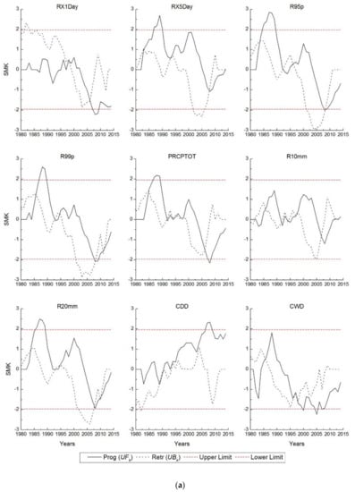
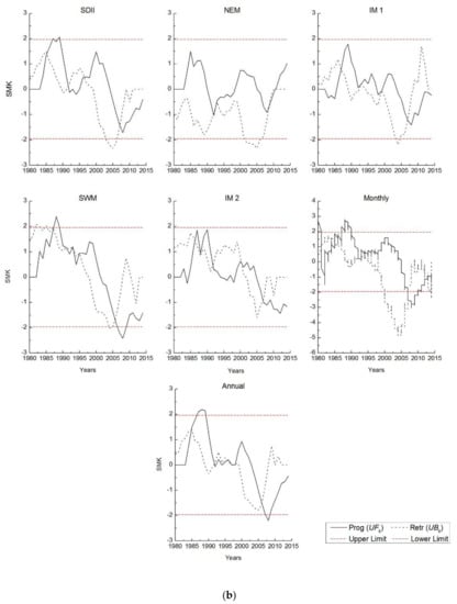
Figure 3. (a) Results of sequential Mann–Kendall test on rainfall indices. (b) Results of sequential Mann–Kendall test on rainfall indices.

The UF_k curves showed the increasing trends for the late 80′s but then started to decrease after 1994–2014. The R10mm did not portray any significant trend as the progressive and retrograded curves cross each other inside the upper and lower limit. It has been mentioned by [43] that if both curves cross each other inside the critical limit, then there is no significant change in the time series. The R20mm also depicted the same trends as R99p, i.e., increasing in the late 1980s and then decreasing trend up to 2014. The results of SMK for CDD, as shown in Figure 3a, indicate the increasing trends of dry spells during the study period with a start from 1989, and the change was significant in 2006. In contrast, the analysis of wet spells has shown declining trends over the state.

Figure 3b presents the results of the SMK test on the seasonal, monthly, and annual rainfall. The analysis of SDII has shown decreasing trends in the precipitation intensity during the entire study period. For NEM, the rainfall trends were increasing in the 80′s; however, they decreased slightly in 1994 and then followed a fairly constant pattern. The same phenomena were observed for IM 1, IM2. However, the UF_k curve of SWM showed the increasing trends from 1980 to 1989, but then it started to decline. The curve crossed the critical value in 2006 and then decreased significantly. For monthly time series, it is evident that a significant increasing trend occurred during the 80s; however, at the end of the twentieth century, the trends started to decrease since 2005. The same phenomenon was observed for annual rainfall as well, which showed the increasing trend in 1986 and then followed the constant pattern. Later, it depicted the decreasing trend in 2007–2008. As for the analysis of all these indices, the abrupt change point was detected at the intersection of UF_k and UB_k curves. It can be observed that almost all the change points have a similar starting time. The change was started in the late 90s over the Perak, and then it started to decrease. With the start of the twenty-first century, the decrease was more obvious in all rainfall indices.

4.3. Variations in the Concentration of Annual Rainfall

Figure 4 compares the results obtained from the PCI analysis of annual rainfall on a decadal basis. The values of PCI vary from 7 to 20 in different regions of Perak over different time spans. As mentioned by the Oliver (1980), the PCI values less than 10 correspond to low rainfall concentration, while the values ranging from 11–15 represent moderate rainfall concentration, and the values from 16–20 indicate the irregular rainfall concentration. Conversely, the values of PCI greater than 20 exhibits a high irregularity in rainfall concentration. As for the explanation, the low concentration of rainfall depicts the uniformity in the rainfall distribution, where the moderate and irregular rainfall concentration represents the seasonality in the rainfall.

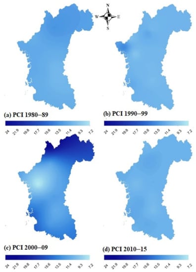
Figure 4. Annual rainfall concentration index on Perak, Malaysia.

As can be seen from Figure 4, the values of PCI from 1980–1989 fluctuated from 10.5–13.1. The lower values were observed over the southeastern regions (i.e., 10.6), while higher values were observed over the northwestern regions, i.e., 13.1 (Figure 4). The same trends were observed for the years 1990–1999. The high concentration values were observed in the western regions, and the lower values were recorded in the southeastern regions. However, the lower values of rainfall concentration were observed over the western regions of Perak for the years 2000–2009. Furthermore, the high irregularity over the northern areas was observed as the recorded value of PCI was 24 (Figure 4). For the last period, PCI values were detected for the half-decade (i.e., 2010–2014) due to the limitation of data. The values of annual PCI stretched from 10 to 11.5 over the western to eastern regions. It can be observed from the figure that the rainfall concentration has gradually shifted from the southeastern regions towards the western regions. The areas of the northeast showed moderate irregularity in rainfall during the entire study period.

4.4. Spatial Distribution of Annual Rainfall

Figure 5 presents the results of the spatial distribution of long-term monthly, seasonal, and annual rainfall over the state from 1980 to 2014. In the case of NEM, the western areas have observed the declination in rainfall with the rate of 0.19 mm/year, while the southeastern areas have experienced an increase in monsoonal rainfall at the rate of 0.56 mm (Figure 5a). The same phenomenon was noted for the IM 1 with the increase in rainfall 1.03 mm (Figure 5b). However, in the case of SWM and IM 2, a decreased rainfall trend was discovered over the entire state. The rate of decrease was higher for the western regions (i.e., 0.45 mm) as compared to the southern regions (i.e., 0.12 mm) for SWM (Figure 5c). Whereas, for IM 2, the rate of decrease was more (i.e., 2.12 mm) from the western regions (Figure 5d). The spatial variability of monthly rainfall has also portrayed the decreased rainfall for the western regions and increased for the southeastern regions (Figure 5e). On an annual basis, again, the trends were similar, and the rate of decrease in annual rainfall was 19 mm for the western regions. On the other hand, the southern regions that are happened to be situated on flat grounds have experienced an increase in rainfall at the rate of 10 mm (Figure 5f).

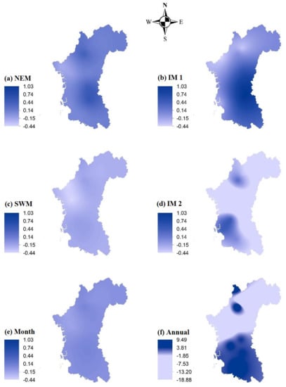
Figure 5. Spatial distribution of long-term (1980–2014) seasonal, monthly, and annual rainfall rates over Perak, Malaysia. The sub-figures (a–d) represents the NEM, IM 1, SWM, and IM2 respectively. The rate of change in seasonal rainfalls are as per the definition given in Table 3, while the sub-figures (e,f) have the units in mm/month and mm/year, respectively.

5. Discussion

Rainfall provides the necessary understanding to quantify the intensity and severity of different hydrological phenomena, such as floods, droughts, river discharge, etc. Estimation of the seasonal and spatial trends of rainfall can offer valuable information not only to the climatic scientists but also to the weather forecasters, hydrologists, and decision-makers. Therefore, the objective of this research was to assess the spatiotemporal trends of rainfall to analyze the problem of recurrent flooding in Perak, Malaysia. The specific objectives were (i) to examine the temporal variability and unexpected trend changes in rainfall indices; and (ii) to ascertain the spatial fluctuations and periodicity in the seasonal and annual rainfall trends.

The purpose of the study was to examine the long-term trends of rainfall on a spatiotemporal scale, but some conclusions can be drawn based on previous research about seasonal and temporal variations in rainfall. Variations in rainfall trends can be related to ambient air temperatures due to the fact that the warmer air holds more moisture than cooler air. Studies have shown a linear relationship between surface air temperature and rainfall. A study found that an increase in surface air temperature due to an increase in the emission of greenhouse gasses (GHGs), ultimately intensified the rainfall pattern over the northern hemisphere during the period from 1950 to 1999 [44]. In this context, another study stated that a change in atmospheric temperature by 7% can significantly increase global rainfall [45]. Despite the fact that these studies were conducted at a global level, some of their effects can be found at the regional level, as observed by other researchers [46].

An increase in dry spells can be explained by the urban heat island (UHI) effect caused by intensive land cover changes. In a previous study, the UHI effect has been shown to cause an increase in atmospheric temperature, particularly in highly populated areas [47]. A recent study analyzing the rate of land-use changes in Perak has mentioned that during the last decade, the land cover has been altered extensively in Perak, Malaysia [27]. The fluctuations in local atmospheric temperatures because of the UHI effect can alter the rainfall over that particular area. This can also be explained by a study done to examine the interannual variation in temperature over entire Malaysia. Their results found that increase in temperature over entire Malaysia is constant because of the El Niño-Southern Oscillation (ENSO) cycle [47]. The ENSO cycle defines the temperature variations of the atmosphere and ocean across the East-central Equatorial Pacific. The variation ultimately directly influences the world’s weather. Another recent study has also indicated that the frequency of wet spells has been decreased significantly from 1971–2010 over entire Peninsular Malaysia because of El Niño events of 1982–1983 and 1997–1998 [48].

Furthermore, a gradually increasing trend in the daily minimum temperature has also been observed by the Malaysian Meteorological department over the entire of Malaysia. A study has directly coincided with the increased trends in temperature with the El Niño events, which occurred in 1972, 1982 and 1997 [49]. On the spatial basis, the variations can be observed over the western regions where rainfall showed decreasing trends and increasing trends over the southeastern regions of the state on a seasonal and annual basis. Recent research has suggested that El Niño and La Niña events affect the rainfall patterns on spatial as well as temporal patterns [50]. The same phenomenon was observed in the analysis of the precipitation concentration index that revealed the convergence of rainfall towards the southeastern regions of Perak from the western regions.

Other studies, such as Manton et al. (2001) and a study by Asian Development Bank have also stated the increase in the sea–level from 1–3 mm/year and a decrease in rainfall since 1960–2000 because of climate change [42]. Even though the results of these studies indicated the decrease in rainfall, their results revealed the increase in hydrological hazards, for instance, floods, droughts, etc., over the Southeast Asian countries. Apart from climate changes, the basic physical properties altered by human activities are also influential in increasing the runoff generation within a watershed. Studies have indicated that factors such as anthropogenic changes also play an important role in flood intensification [51]. Anthropogenic changes can be attributed to deforestation, expansion of croplands, industrialization, and urbanization that consequently disrupts the river hydrology by reducing the infiltration and water holding capacity of the river plain. World Meteorological Organization has also stated that human activities, for instance, deforestation and urbanization have strongly influenced the biotic diversity of the globe. These changes in the ecosystem would subsequently lead to increased precipitation, which will result in more severe flooding [52]. The results obtained from the analysis of rainfall indices over Perak have revealed that the recent flooding was not solely due to climatic changes. Therefore, for sustainable spatial future planning, consideration of other factors such as deforestation, dam breakage, etc., will also help to identify the root causes of flood intensification.

6. Conclusions

This study aimed to evaluate the spatiotemporal trends of rainfall over the state of Perak Malaysia during the last 35 years. Trends in extreme rainfall indices along with the seasonal and annual rainfall were examined. The most obvious finding to emerge from the study was significant decreasing trends in the Southwest Monsoon (SWM) rainfall during the study period of 1980–2014. The study has also shown that most of the rainfall indices are following insignificant decreasing trends. From the results, it was evident that the decreasing point extreme indices were observed starting from 2005. On the spatial level, the rainfall depicted the convergence from the western regions towards the north-eastern regions that are highly populated areas. The analysis of threshold rainfall indices (R99p and R95p) for flooding intensification did not portray any significant increasing trends, which imply the possibility of other factors in flood intensification. In general, it can be concluded that rainfall over Perak, Malaysia, is following a slightly decreasing trend. The results of this study can be extended to understand the regional flooding over the Perak. A further study with more rainfall datasets focusing on the impact assessment of El Niño, global warming, and land-use changes on regional climate and the hydrological cycle is therefore suggested.

References

- Treloar, N.C. Deconstructing Global Temperature Anomalies: An Hypothesis. Climate 2017, 5, 83. [Google Scholar] [CrossRef] [Green Version]
- Mahmood, R.; Babel, M.S. Evaluation of SDSM developed by annual and monthly sub-models for downscaling temperature and precipitation in the Jhelum basin, Pakistan and India. Theor. Appl. Climatol. 2013, 113, 27–44. [Google Scholar] [CrossRef]
- Masson-Delmotte, V.P.; Zhai, A.; Pirani, S.L.; Connors, C.; Péan, S.; Berger, N.; Caud, Y.; Chen, L.; Goldfarb, M.I.; Gomis, M.; et al. (Eds.) IPCC, 2021: Climate Change 2021: The Physical Science Basis. Contribution of Working Group I to the Sixth Assessment Report of the Intergovernmental Panel on Climate Change; Cambridge University Press: Cambridge, UK, 2021. [Google Scholar]
- Yang, S.; Kang, T.; Bu, J.; Chen, J.; Gao, Y. Evaluating the Impacts of Climate Change and Vegetation Restoration on the Hydrological Cycle over the Loess Plateau, China. Water 2019, 11, 2241. [Google Scholar] [CrossRef] [Green Version]
- Tanteliniaina, M.F.R.; Chen, J.; Adyel, T.M.; Zhai, J. Elevation Dependence of the Impact of Global Warming on Rainfall Variations in a Tropical Island. Water 2020, 12, 3582. [Google Scholar] [CrossRef]
- Huang, P.; Xie, S.-P.; Hu, K.; Huang, G.; Huang, R. Patterns of the seasonal response of tropical rainfall to global warming. Nat. Geosci. 2013, 6, 357–361. [Google Scholar] [CrossRef]
- Liaqat, M.U.; Grossi, G.; Hasson, S.u.; Ranzi, R. Characterization of interannual and seasonal variability of hydro-climatic trends in the Upper Indus Basin. Theor. Appl. Climatol. 2022, 147, 1163–1184. [Google Scholar] [CrossRef]
- Nalley, D.; Adamowski, J.; Khalil, B. Using discrete wavelet transforms to analyze trends in streamflow and precipitation in Quebec and Ontario (1954–2008). J. Hydrol. 2012, 475, 204–228. [Google Scholar] [CrossRef]
- Stocker, T. Climate Change 2013: The Physical Science Basis: Working Group I Contribution to the Fifth Assessment Report of the Intergovernmental Panel on Climate Change; Cambridge University Press: Cambridge, UK, 2014. [Google Scholar]
- Solomon, S.; Manning, M.; Marquis, M.; Qin, D. Climate Change 2007—The Physical Science Basis: Working Group I Contribution to the Fourth Assessment Report of the IPCC; Cambridge University Press: Cambridge, UK, 2007; Volume 4. [Google Scholar]
- Lau, C.L.; Smythe, L.D.; Craig, S.B.; Weinstein, P. Climate change, flooding, urbanisation and leptospirosis: Fuelling the fire? Trans. R. Soc. Trop. Med. Hyg. 2010, 104, 631–638. [Google Scholar] [CrossRef]
- Hirabayashi, Y.; Mahendran, R.; Koirala, S.; Konoshima, L.; Yamazaki, D.; Watanabe, S.; Kim, H.; Kanae, S. Global flood risk under climate change. Nat. Clim. Chang. 2013, 3, 816–821. [Google Scholar] [CrossRef]
- Kia, M.B.; Pirasteh, S.; Pradhan, B.; Mahmud, A.R.; Sulaiman, W.N.A.; Moradi, A. An artificial neural network model for flood simulation using GIS: Johor River Basin, Malaysia. Environ. Earth Sci. 2012, 67, 251–264. [Google Scholar] [CrossRef]
- Pradhan, B. Flood susceptible mapping and risk area delineation using logistic regression, GIS and remote sensing. J. Spat. Hydrol. 2010, 9, 1–18. [Google Scholar]
- Chan, N.W. Impacts of disasters and disaster risk management in Malaysia: The case of floods. In Resilience and Recovery in Asian Disasters; Springer: Berlin/Heidelberg, Germany, 2015; pp. 239–265. [Google Scholar]
- Brakenridge, G.; Anderson, E. Satellite-Based Inundation Vectors; Dartmouth Flood Observatory, Dartmouth College: Hanover, LS, USA, 2004. [Google Scholar]
- Pathak, P.; Kalra, A.; Ahmad, S. Temperature and precipitation changes in the Midwestern United States: Implications for water management. Int. J. Water Resour. Dev. 2017, 33, 1003–1019. [Google Scholar] [CrossRef]
- Pérez-Zanón, N.; Casas-Castillo, M.C.; Rodríguez-Solà, R.; Peña, J.C.; Rius, A.; Solé, J.G.; Redaño, Á. Analysis of extreme rainfall in the Ebre Observatory (Spain). Theor. Appl. Climatol. 2016, 124, 935–944. [Google Scholar] [CrossRef] [Green Version]
- Liu, Z. Evaluation of precipitation climatology derived from TRMM Multi-Satellite Precipitation Analysis (TMPA) monthly product over land with two gauge-based products. Climate 2015, 3, 964–982. [Google Scholar] [CrossRef] [Green Version]
- Ahmad, I.; Zhang, F.; Tayyab, M.; Anjum, M.N.; Zaman, M.; Liu, J.; Farid, H.U.; Saddique, Q. Spatiotemporal analysis of precipitation variability in annual, seasonal and extreme values over upper Indus River basin. Atmos. Res. 2018, 213, 346–360. [Google Scholar] [CrossRef]
- Krebs, G.; Camhy, D.; Muschalla, D. Hydro-Meteorological Trends in an Austrian Low-Mountain Catchment. Climate 2021, 9, 122. [Google Scholar] [CrossRef]
- Obubu, J.P.; Mengistou, S.; Fetahi, T.; Alamirew, T.; Odong, R.; Ekwacu, S. Recent Climate Change in the Lake Kyoga Basin, Uganda: An Analysis Using Short-Term and Long-Term Data with Standardized Precipitation and Anomaly Indexes. Climate 2021, 9, 179. [Google Scholar] [CrossRef]
- Wong, C.; Venneker, R.; Uhlenbrook, S.; Jamil, A.; Zhou, Y. Variability of rainfall in Peninsular Malaysia. Hydrol. Earth Syst. Sci. Discuss. 2009, 6, 5471–5503. [Google Scholar]
- Suhaila, J.; Jemain, A.A. Spatial analysis of daily rainfall intensity and concentration index in Peninsular Malaysia. Theor. Appl. Climatol. 2012, 108, 235–245. [Google Scholar] [CrossRef]
- Amirabadizadeh, M.; Huang, Y.F.; Lee, T.S. Recent trends in temperature and precipitation in the Langat River Basin, Malaysia. Adv. Meteorol. 2015, 2015, 579437. [Google Scholar] [CrossRef] [Green Version]
- Chabala, L.M.; Kuntashula, E.; Kaluba, P. Characterization of temporal changes in rainfall, temperature, flooding hazard and dry spells over Zambia. Univers. J. Agric. Res. 2013, 1, 134–144. [Google Scholar] [CrossRef]
- Hanif, M.F.; ul Mustafa, M.R.; Hashim, A.M.; Yusof, K.W. Spatio-temporal change analysis of Perak river basin using remote sensing and GIS. In Proceedings of the 2015 International Conference on Space Science and Communication (IconSpace), Langkawi, Malaysia, 10–12 August 2015; pp. 225–230. [Google Scholar]
- Bargaoui, Z.K.; Chebbi, A. Comparison of two kriging interpolation methods applied to spatiotemporal rainfall. J. Hydrol. 2009, 365, 56–73. [Google Scholar] [CrossRef]
- Verdin, A.; Funk, C.; Rajagopalan, B.; Kleiber, W. Kriging and local polynomial methods for blending satellite-derived and gauge precipitation estimates to support hydrologic early warning systems. IEEE Trans. Geosci. Remote Sens. 2016, 54, 2552–2562. [Google Scholar] [CrossRef]
- Stefanidis, S.; Stathis, D. Spatial and temporal rainfall variability over the Mountainous Central Pindus (Greece). Climate 2018, 6, 75. [Google Scholar] [CrossRef] [Green Version]
- Oliver, J.E. Monthly precipitation distribution: A comparative index. Prof. Geogr. 1980, 32, 300–309. [Google Scholar] [CrossRef]
- de Luis, M.; Gonzalez-Hidalgo, J.; Brunetti, M.; Longares, L. Precipitation concentration changes in Spain 1946–2005. Nat. Hazards Earth Syst. Sci. 2011, 11, 1259–1265. [Google Scholar] [CrossRef] [Green Version]
- Thomas, J.; Prasannakumar, V. Temporal analysis of rainfall (1871–2012) and drought characteristics over a tropical monsoon-dominated State (Kerala) of India. J. Hydrol. 2016, 534, 266–280. [Google Scholar] [CrossRef]
- Sayemuzzaman, M.; Jha, M.K. Seasonal and annual precipitation time series trend analysis in North Carolina, United States. Atmos. Res. 2014, 137, 183–194. [Google Scholar] [CrossRef]
- Yue, S.; Pilon, P.; Cavadias, G. Power of the Mann–Kendall and Spearman’s rho tests for detecting monotonic trends in hydrological series. J. Hydrol. 2002, 259, 254–271. [Google Scholar] [CrossRef]
- Önöz, B.; Bayazit, M. Block bootstrap for Mann–Kendall trend test of serially dependent data. Hydrol. Processes 2012, 26, 3552–3560. [Google Scholar] [CrossRef]
- Kendall, M.G. Rank Correlation Methods; University of Michigan: Ann Arbor, MI, USA, 1948. [Google Scholar]
- Mann, H.B. Nonparametric tests against trend. Econom. J. Econom. Soc. 1945, 13, 245–259. [Google Scholar] [CrossRef]
- Mohsin, T.; Gough, W.A. Trend analysis of long-term temperature time series in the Greater Toronto Area (GTA). Theor. Appl. Climatol. 2010, 101, 311–327. [Google Scholar] [CrossRef]
- Quansah, J.E.; Naliaka, A.B.; Fall, S.; Ankumah, R.; Afandi, G.E. Assessing Future Impacts of Climate Change on Streamflow within the Alabama River Basin. Climate 2021, 9, 55. [Google Scholar] [CrossRef]
- Amarouche, K.; Akpınar, A. Increasing Trend on Storm Wave Intensity in the Western Mediterranean. Climate 2021, 9, 11. [Google Scholar] [CrossRef]
- Manton, M.J.; Della-Marta, P.M.; Haylock, M.R.; Hennessy, K.; Nicholls, N.; Chambers, L.; Collins, D.; Daw, G.; Finet, A.; Gunawan, D. Trends in extreme daily rainfall and temperature in Southeast Asia and the South Pacific: 1961–1998. Int. J. Climatol. 2001, 21, 269–284. [Google Scholar] [CrossRef]
- Guo, L.; Xia, Z. Temperature and precipitation long-term trends and variations in the Ili-Balkhash Basin. Theor. Appl. Climatol. 2014, 115, 219–229. [Google Scholar] [CrossRef]
- Min, S.-K.; Zhang, X.; Zwiers, F.W.; Hegerl, G.C. Human contribution to more-intense precipitation extremes. Nature 2011, 470, 378–381. [Google Scholar] [CrossRef]
- Westra, S.; Alexander, L.V.; Zwiers, F.W. Global increasing trends in annual maximum daily precipitation. J. Clim. 2013, 26, 3904–3918. [Google Scholar] [CrossRef] [Green Version]
- Sato, T.; Kimura, F.; Kitoh, A. Projection of global warming onto regional precipitation over Mongolia using a regional climate model. J. Hydrol. 2007, 333, 144–154. [Google Scholar] [CrossRef]
- Tangang, F.; Juneng, L.; Ahmad, S. Trend and interannual variability of temperature in Malaysia: 1961–2002. Theor. Appl. Climatol. 2007, 89, 127–141. [Google Scholar] [CrossRef]
- Zin, W.Z.W.; Jamaludin, S.; Deni, S.M.; Jemain, A.A. Recent changes in extreme rainfall events in Peninsular Malaysia: 1971–2005. Theor. Appl. Climatol. 2010, 99, 303–314. [Google Scholar] [CrossRef]
- Sammathuria, M.; Ling, L. Regional climate observation and simulation of extreme temperature and precipitation trends. In Proceedings of the 14th International Rainwater Catchment Systems Conference, Kuala Lumpur, Malaysia, 3–6 August 2009; pp. 3–6. [Google Scholar]
- Portmann, R.W.; Solomon, S.; Hegerl, G.C. Spatial and seasonal patterns in climate change, temperatures, and precipitation across the United States. Proc. Natl. Acad. Sci. USA 2009, 106, 7324–7329. [Google Scholar] [CrossRef] [PubMed] [Green Version]
- Kundzewicz, Z.; Schellnhuber, H.-J. Floods in the IPCC TAR perspective. Nat. Hazards 2004, 31, 111–128. [Google Scholar] [CrossRef]
- Ramesh, A. Response of Flood Events to Land Use and Climate Change: Analyzed by Hydrological and Statistical Modeling in Barcelonnette, France; Springer Science & Business Media: Berlin/Heidelberg, Germany, 2012. [Google Scholar]
Publisher’s Note: MDPI stays neutral with regard to jurisdictional claims in published maps and institutional affiliations. |
© 2022 by the authors. Licensee MDPI, Basel, Switzerland. This article is an open access article distributed under the terms and conditions of the Creative Commons Attribution (CC BY) license (https://creativecommons.org/licenses/by/4.0/).