Article

Modelling of Extremely High Rainfall in Limpopo Province of South Africa

by
Thendo Sikhwari
1,†,
Nthaduleni Nethengwe
1,
Caston Sigauke
2,*,† and
Hector Chikoore
3
1
Department of Geography and Geo-Information Sciences, School of Environmental Sciences, University of Venda, Thohoyandou 0950, South Africa
2
Department of Mathematical and Computational Sciences, University of Venda, Private Bag X5050, Thohoyandou 0950, South Africa
3
Unit for Environmental Science and Management, North West University, Vanderbijlpark 1900, South Africa
*
Author to whom correspondence should be addressed.
These authors contributed equally to this work.
Climate 2022, 10(3), 33; https://doi.org/10.3390/cli10030033
Submission received: 24 January 2022 / Revised: 15 February 2022 / Accepted: 21 February 2022 / Published: 28 February 2022
(This article belongs to the Special Issue Extreme Weather Events)

Abstract

:
Extreme value theory is a powerful method that is known to provide statistical models for events rarely observed. This paper presents a modelling framework for the maximum rainfall data recorded in Limpopo province, South Africa, from 1960 to 2020. Daily and monthly rainfall data were obtained from the South Africa Weather Service. In this work, the r-largest order statistics modelling approach is used. Yearly blocks were used in fitting a 61 years’ data set. The parameters of the developed models were estimated using the maximum likelihood method. After the suitable model for data was chosen, i.e., GEVD r = 8 , the 50-year return level was estimated as 368 mm, which means a probability of 0.02 exceeding 368 mm in fifty years in the Thabazimbi area. This study helps decision-makers in government and non-profit organisations improve preparation strategies and build resilience in reducing disasters resulting from extreme weather events such as excessive rainfall.

1. Introduction

Climate extremes such as floods, droughts and heatwaves have become topical issues since they have triggered most natural disasters in recent decades that can potentially affect humans and the natural environment [1]. Climate extreme events are regular across the globe and impact society in various ways, leading to loss of lives, shortage of food, failure of crops, famine, mass migration and health issues [2]. The increased number, frequency and intensity of natural hazards such as floods, heatwaves and hurricanes are generally attributed to climate change [3,4,5]. In Africa, impacts of a changing climate vary significantly by region [6,7]. More than 90% of natural disasters in southern Africa are related to weather, climate and water. Understanding extreme climate events will help prepare and formulate mitigation strategies to cope with events associated with climate change. Modelling and predicting future extreme events become more relevant in commercial agriculture, to insurance companies, statisticians and meteorologists.
Extreme climate and weather events such as floods, droughts and heatwaves negatively impact society, environment and resource management in developing countries [6,8,9]. In South Africa, anomalous cut-off lows, tropical cyclones and tropical storms are the major extreme rainfall producing systems affecting the Limpopo province, while the Botswana High becomes dominant during heatwaves and drought. Extreme weather events are common in Limpopo during summertime and often coincide with mature phases of the El Niño Southern Oscillation. In February 2000, about 700 people lost their lives and over a million residents were displaced in Mozambique due to flooding associated with tropical cyclone Eline [10,11]. In recent decades (1980–2015), southern Africa experienced 491 climate disasters (hydrological, climatological and meteorological) which resulted in 110,978 deaths and left 2.49 million people homeless [8,12]. Therefore, climate extreme events cause risks to the lives and livelihoods of South African society [13]. South Africa is highly vulnerable to extreme climate events due to its geographical location and socio-economic factors. Several tropical cyclones have distressed various countries such as Madagascar, Mozambique and South Africa [14].
Rainfall is highly variable over southern Africa on several space and time scales [15]. Climate change has altered rainfall characteristics, including duration of the rainy season, the length of dry spells, frequency of rainy days and the occurrence of heavy rainfall events [16]. This results in regular and severe water-associated extremes such as floods and drought [17]. In South Africa, the Limpopo province experiences hot to very hot conditions during the austral summer season [18,19]. Extreme drought is a critical problem in the region affecting the agricultural sector due to high temperatures and unreliable rainfall [8,20]. This study is built on this factual background coupled with challenges and impacts of climate and weather extreme events in the Limpopo province.
Long-term data gained from historical extreme climate analysis provides a huge possibility for good management, forecasting and mitigation of climate extremes [7]. Extreme Value Theory is a powerful method to quantify the stochastic behaviour of low or unusual levels. Extreme value theory (EVT) has been widely used in various fields such as atmospheric science (e.g., [21]), hydrology (e.g., [22]), finance industry [23] and many other fields of application. The observational and statistical modelling results of the studies mentioned above have shown remarkable increases in the intensity of precipitation extremes.
This study aimed to employ Extreme Value Theory to model climate extreme events in the future using generalised extreme value distribution (GEVD) by using the maximum likelihood estimation method. Generalised extreme value distribution (GEVD) is the family of asymptotic distribution that describes the behaviour of extreme conditions. The GEVD consists of three extreme value distributions, namely: Gumbel, Fréchet and Weibull families, which are also referred to as type I, II and III extreme value distributions [24].
Chifurira and Chikobvu [25] fitted a GEVD to average yearly rainfall with an objective of modelling the upper tail of the rainfall distribution. The Gumbel class of distributions was found to fit the data well using the Anderson–Darling goodness of fit test. The GEVD with constant shape and scale parameters but varying location parameters over time were inadequate to model Zimbabwe’s extreme maximum rainfall. The study indicated that a high mean annual rainfall of 1193 mm is expected in approximately 300 years ([25]). A similar analysis to the present study in multivariate extreme value theory (MEVT) is that of [26], who used bivariate threshold excess in modelling temperature extremes in the Limpopo province for three meteorological stations Thohoyandou, Lephalale and Polokwane. Similar to the present study, the approach by [26] also used a penalised cubic smoothing spline to perform a nonlinear detrending of the temperature data before fitting bivariate threshold excess models to positive residuals above the threshold. The present study dealing with rainfall as the main parameter extends the approach of [26] by using a time-varying threshold instead of a constant threshold to capture the climate change effects in the monthly maximum rainfall data series. Recent studies on modelling extreme rainfall using extreme value theory and the r-largest order statistics considering model and return level uncertainty include those of [27,28,29], among others.
This study applies extreme value distribution to model maximum annual rainfall in Limpopo province. Results from this study can contribute vitally to the knowledge of EVT application to long-term rainfall data and recommendations to government agencies private organisations on extreme events and their negative impact on the economy. There are no studies available to the public domain in the science sphere that have modelled long-term yearly maximum rainfall in Limpopo province using EVT approaches applied in this study.
Various studies such as [30] discuss the modelling of the influence of temperature on average daily electricity demand in South Africa using a piecewise linear regression model and the generalised extreme value theory approach from 2000–2010. Severe weather conditions increase electricity demand because air-conditioned appliances are used in summer and heating systems are used in winter [6,30]. South Africa is also concerned about the impacts of extreme heat wave events on the public and how these events may change in the future [31,32]. The most robust approach in Extreme Value Theory is the choice of a threshold when using the POT approach. We also closely follow the work of [33,34].
Southworth et al. [34] provide a detailed computational approach of multivariate extreme value data conditional modelling using an R package called ‘texmex’. In another study on threshold choice, Ref. [
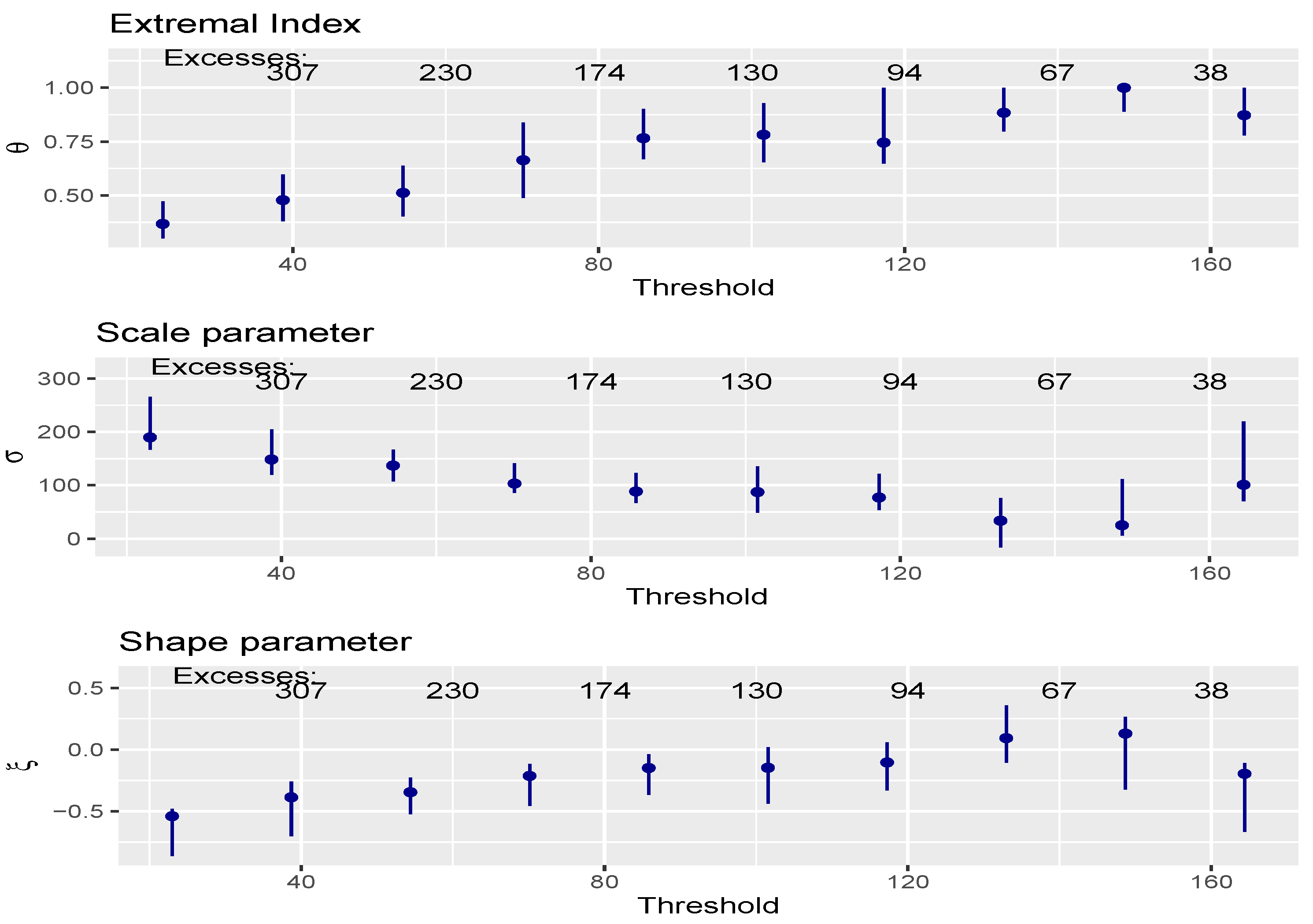
35] proposed a covariate-dependent threshold based on expectiles. They argued that although no threshold choice method is universally the best, strong arguments against the use of constant threshold is that the observation that may be considered extreme at some covariate level may not necessarily qualify as an extreme observation when considered at another covariate level. The present study use threshold stability plots. This is a graphical method that is widely used to determine the threshold. The idea of this plot is that the exceedances of a high threshold follow a GPD. The study by [36] used a GPD with time-varying covariates and thresholds to model daily peak electricity demand for South Africa. They used an intervals estimator method in declustering observations that exceed the threshold. Furthermore, the findings of [36] showed a better fit for the GPD model to the data compared to the generalised extreme value distribution (GEVD).
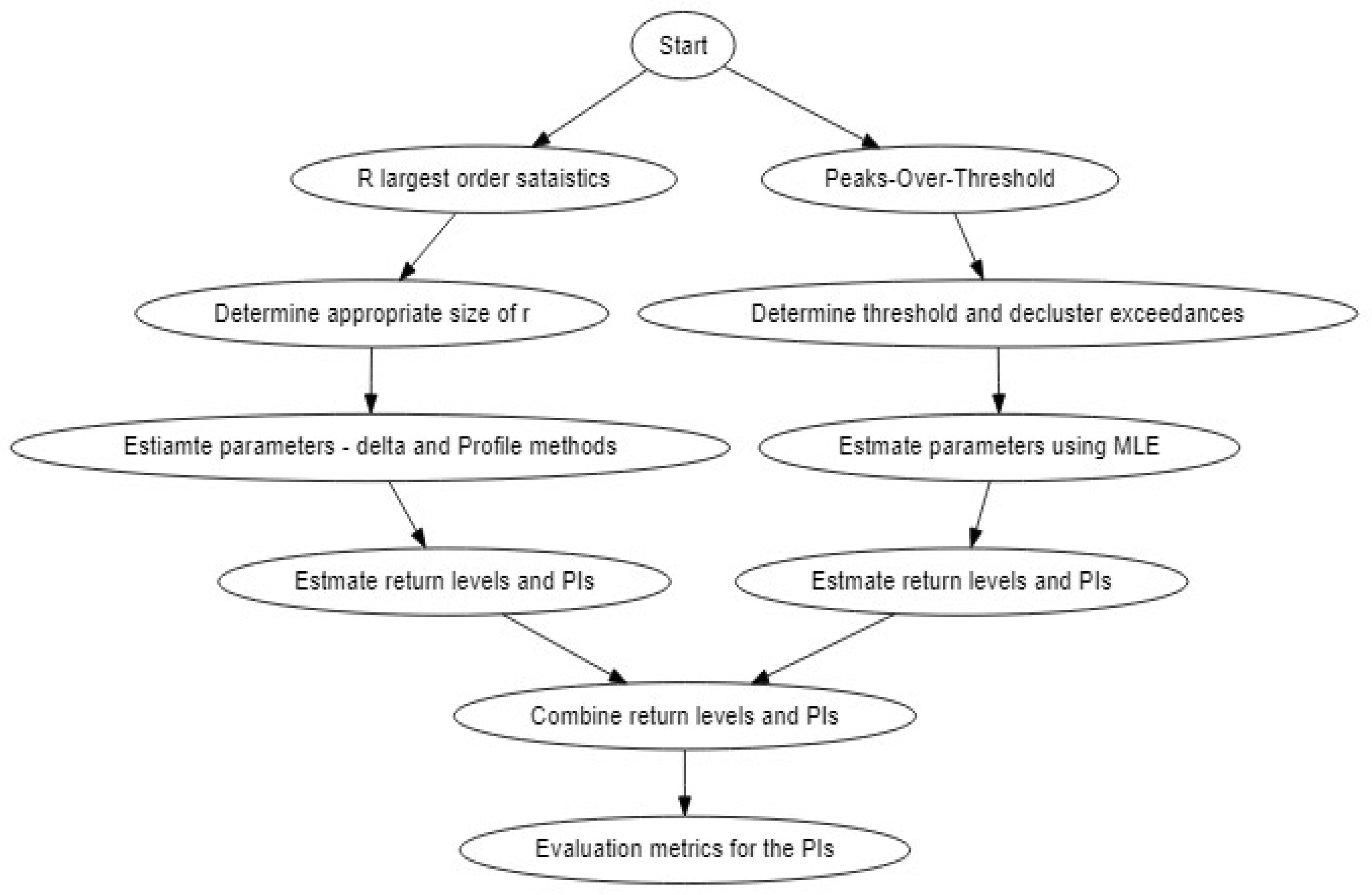
The main highlights of this study are as follows: The main contribution of this paper is to employ Extreme Value Theory to model climate extreme events using the r-largest order statistics. The knowledge and understanding of extreme climate events will help prepare and formulate mitigation strategies to cope with events associated with climate change. In this study, the interest was in deriving extreme maximum rainfall return levels from 1960 to 2020. The study combines two main approaches: bivariate condition extremes model [33,34,37] and time-varying threshold [36]. The rest of the paper is organised as follows: Section 2 presents the materials and methods. The empirical results are presented in Section 3. A discussion of the results is given in Section 4, while Section 5 concludes the paper.

2. Materials and Methods

Extreme Value Theory (EVT) is unique as a statistical discipline in that it develops techniques and models for describing the unusual rather than the usual [38]. EVT was used in the modelling of extreme rainfall. The analysis of extremes for a given data representing extremes was selected. EVT provides a tool for modelling the asymptotic distribution of a sequence of observations [39]. The best way to describe the behaviour of climate extreme events for a particular environment is to identify the distribution(s) suitable to fit the data. In this study, the generalised Pareto distribution (GPD) was used for estimating extreme return levels of historical monthly rainfall data from 1960 to 2020.

2.1. The r-Largest Order Statistics

The use of r-largest order statistics is usually used with limited data. This study is motivated by the desire to search for characterisation of extreme value behaviour other than using one observation in a block that would enable modelling observations in the upper tails of distributions. Such an approach is more efficient in its use of data.
Let X 1 , X 2 , . . . , X n , be a sequence of independent and identically distributed (i.i.d.) random variables. Define M n ( k ) = k th largest of { X 1 , . . . , X n } . If there exists a sequence of constants { a n > 0 } and { b n > 0 } such that: P M n ( r ) b n a n z G ( z ) as n for some non degenerate distribution G, then, for fixed r, the limiting distribution as n of M ˜ n ( r ) = M n ( 1 ) b n a n , . . . , M n ( r ) b n a n falls within the family having joint probability density function (for ξ 0 ) [38].
f x ( 1 ) , . . . , x ( r ) = exp 1 + ξ x ( r ) μ σ 1 ξ × k = 1 r 1 σ 1 + ξ x ( k ) μ σ 1 ξ 1 ,
where < μ < , σ > 0 and < ξ < ; x ( r ) x ( r 1 ) . . . x ( 1 ) ; and x ( k ) : 1 + ξ x ( k ) μ σ > 0 for k = 1 , 2 , . . . , r . For the case r = 1 , we have the GEVD model. When ξ 0 usually written as ξ = 0 , the joint density is given as:
f x ( 1 ) , . . . , x ( r ) = exp exp x ( r ) μ σ × k = 1 r 1 σ x ( k ) μ σ .
Equation (2) reduces to the Gumbel class of distributions when r = 1 . Selection of the best value of r in this study is done using the automatic selection algorithm discussed in [40].

2.2. Peaks-over-Threshold Approach

2.2.1. The Generalised Pareto Distribution

The Generalised Pareto Distribution (GPD) is a Peaks-over-threshold (POT) distribution that can be used to model the observations above a sufficiently high threshold [41]. The GPD has two parameters ξ , the shape parameter, and σ , the scale parameter.
The survival function of the GPD is given in Equation (3).
P ( X > x | τ ) = 1 + ξ ( x τ ) σ 1 ξ if ξ > 0 , x τ > 0 exp x τ σ , if ξ = 0 , x τ > 0 1 + ξ ( x τ ) σ 1 ξ if ξ < 0 , 0 < x τ < σ ξ
Equation (3) shows that when ξ < 0 the survival function of the GPD is bounded above by σ ξ . The return levels are estimated using Equation (4)
x p = τ + σ ξ p ξ 1 , ξ 0 , x > τ

2.2.2. Threshold Selection and Declustering

In this paper, we use threshold stability plots. The procedure of declustering and then fitting the GPD to cluster maxima gives a valid statistical model whose underlying assumptions are met. However, the cluster maxima may not be of ultimate interest in practice. For example, rainfall information can be helpful if the assessment of flood damage is the ultimate goal. Here it may be more informative to analyse complete clusters and understand the aggregate rainfall over a rainy spell, rather than focus on the largest yearly value over that spell [42]. In this paper, the declustering approach proposed by [43] is used. This problem is inherently more difficult and requires a much more sophisticated solution; this paper does not attempt such.

2.3. Parameter Estimation

In this paper, we are going to use the MLE.

2.3.1. The Delta Method

Using the delta method the variance of x p is given as [38,44]:
Var ( x ^ p ) x p T V x p ,
where V is the covariance matrix of μ ^ , σ ^ , ξ ^ and
x p T = x p μ , x p σ , x p ξ = [ 1 , ξ 1 1 y p ξ , σ ξ 2 1 y p ξ σ ξ 1 y p ξ log y p ] ,
which is evaluated at μ ^ , σ ^ , ξ ^ . The approximate confidence interval of the flood heights x p is then given by
x ^ p z α / 2 Var ( x ^ p ) , x ^ p + z α / 2 Var ( x ^ p ) .

2.3.2. The Profile Likelihood Method

The profile likelihood for some parameter θ i is defined as [38]:
( θ i ) = max ( θ i , θ i ) ,
where θ i represents components of θ excluding θ i [38,44]. To obtain the confidence interval for x p a re-parametrisation is required in which x p is one of the parameters in the GEVD r model, given as follows:
μ = x p σ ^ ξ ^ 1 y p ξ ^ , if ξ 0 x p σ ^ log y p if ξ = 0 ,
with y p = log ( 1 p ) .

2.4. Forecast Combination

2.4.1. Combining Estimated Return Levels and Prediction Intervals

The idea of combining forecasts was first developed by [45]. They argued that combined forecasts improve forecast over the single model forecast. Suppose the estimated return levels from G E V D r = 1 , G E V D r > 1 and   G P D models are combined so that we have a vector
y ^ r l = y ^ r l ( G E V D r = 1 ) , y ^ r l ( G E V D r > 1 ) , y ^ r l ( G P D )
In this study the estimated return levels will be combined using the simple average and median methods. The average method is given as:
y ^ r l ( a v e ) = i = 1 M y ^ r l , i M
and the median method as
y ^ r l ( m e d ) = Median y ^ r l ( G E V D r = 1 ) , y ^ r l ( G E V D r > 1 ) , y ^ r l ( G P D )
Robust prediction intervals (PIs) is known to be produced from combining prediction limits from various models ([46,47,48]; among others). In this study we shall use the simple average and median methods for combining the prediction limits. The simple average method can be expressed as in Equation (13).
L A v = 1 m t = 1 m L t U A v = 1 m t = 1 m U t
The median method is known to be less sensitive to outliers. This is given in Equation (14)
L M d = Median ( L 1 , , L m ) U M d = Median ( U 1 , , U m )

2.4.2. Evaluation of Prediction Intervals

The models used in this study are only a simplification and approximation of the actual rainfall behaviour (patterns). The first index for estimating PI is the prediction interval width (PIW). It is estimated using lower and upper prediction limits and calculated as shown in Equation (15).
P I W t = U α ( y t ) L α ( y t ) t = 1 , , m
where U α ( y t )   and   L α ( y t ) , denote the upper and lower prediction limits respectively, and α is the nominal confidence.
The quality of the PIs is evaluated using various indices such as the prediction interval coverage probability (PICP), prediction interval normalised average width (PINAW), among others. This study uses the PINAW. PINAW indicates the model’s ability to capture the uncertainty information on the interval predictions. It evaluates the average width of the PIs and is given as
PINAW = 1 m R t = 1 m P I W t ,
where R is the range of the variable y t . A smaller PINAW means the PIs are more informative.
The flow chart of the proposed modelling framework is given in Figure 1.

2.5. Data and Study Area

2.5.1. Description of the Study Area

South Africa is a semi-arid country, receiving annual rainfall of about 464 mm on average, compared to the global average of 860 mm. Large parts of South Africa receive rainfall during the austral summer season. However, the southwestern Cape receives predominantly winter rainfall, with all-year rainfall over the Cape south coast. This study focuses on the Limpopo province, located on the northeast of South Africa and neighbouring Zimbabwe, Mozambique and Botswana. The province falls within the summer-rainfall region (October to March) and thunderstorms are common during the day. Very little rainfall is received during the austral winter.
The southern part of Limpopo lies on the African plateau, while the north eastern Lowveld is well below 1000 m in the Limpopo River valley (see Figure 2). The elevated interior, the low-altitude coastal plain and mountain systems are the three basic landforms of southern Africa. The terrain enhances rainfall by causing the orographic uplift of warm moist air.

2.5.2. Rainfall

In this study, daily rain gauge observations from several stations in Limpopo were obtained from the South African Weather Service (SAWS) for the period 1960–2020. The observations are made once every 24 h at 6.00Z (8:00 am South Africa Standard Time). This study selected Thabazimbi station with at least 95% rainfall data from 1960 to 2020 over Limpopo province. Due to lack of long-term data from other meteorological stations, other stations were excluded in this study. The data is recorded uniformly in all stations as per the World Meteorological Organisation (WMO) guidelines. The observations are made simultaneously across the southern African region to allow inter-comparisons. Table 1 shows a summary of the information about the Thabazimbi weather station.

2.5.3. El Niño Southern Oscillation Indices

Seasonal rainfall over southern Africa has been related to the El Niño Southern Oscillation (ENSO). The phase and strength of El Niño and La Niña events may be measured using the Southern Oscillation Index (SOI) or Niño 3.4 Index. The SOI measures the standardised pressure difference between Tahiti in the central Pacific and Darwin in northern Australia [49]. The Niño 3.4 Index is a measure of sea surface temperature anomalies in the eastern equatorial Pacific. The SOI indices were obtained from the archives of NCEP and were correlated with rainfall over the Limpopo province.

2.5.4. Indian Ocean Dipole

In addition to ENSO, Indian Ocean Dipole (IOD) is another phenomenon which allows for the interaction between the atmosphere and the sea and is referred to as the IOD [50]. Positive IOD, when the SSTs in the western Indian Ocean are warmer relative to the east, dominates the enhancement of rainfall over eastern Africa [51]. Negative IOD, when the western Indian Ocean is cooler relative to the east, is normally associated with wet conditions over the south-eastern part of southern Africa. IOD is partly responsible for driving climate variability of surrounding landmasses and is related to the El Niño Oscillation system [52]. Mondal and Mujumdar [53] used EVT to analyse characteristic changes in extreme rainfall in India using a high-resolution daily gridded dataset. Non-stationary distributions with varying parameters for physical covariates like ENSO-index, global average temperature and local mean temperatures were used to model intensity, duration and frequency of extreme rainfall over a high threshold. Intensity, duration and frequency were non-stationary and no spatially uniform pattern was found in their changes across India. Period of excessive rain was found to be stationary in most of the locations in India. In contrast, associations between frequency, intensity and local temperature changes were found to be non-stationary [53,54].

3. Results

In this section, we discuss the empirical results of the study.

3.1. Exploratory Data Analysis

For the case r = 1 , we used annual blocks to extract the maximum monthly values each year. The data is then called the annual maximum rainfall (AMR). For the case r > 1 , we used the automatic selection algorithm discussed in [40]. The monthly rainfall (MR) data is used with the peaks-over-threshold model, the generalised Pareto distribution (GPD).
Table 2 shows summary statistics of both MR and AMR data sets. Over the sampling period the monthly maximum is the same as the annual maximum, which is the maximum rainfall over the sampling period.
Figure 3 shows a scatter plot of the monthly rainfall over the sampling period.
Initially, the data were tested for the existence of a monotonic trend using the Cox–Stuart (CS) trend test. Using the CS test, the p-value was 0.2492, implying no monotonic trend at the 5% level of significance. However, on using the Mann–Kendall (MK) trend test and the seasonal MK test, we failed to reject the null hypothesis and concluded that there is both a local trend (p-value = 0.0001784) and a seasonal global trend (p-value = 0.000002689). This was then followed by computing the magnitude of the trend based on Sen’s slope test. The sample estimate of the slope was found to be −0.0041841 with a 95% confidence interval of (−0.0163, 0.0000). The seasonal Sen’s slope was estimated as zero. The magnitudes of both the local trend slope and the seasonal slope are very small. The correlation between the rainfall data with Soi and IOD data was weak. As a result, these two variables were not included as covariates in the developed models.

3.2. GEVD r Results

The tests were carried out on the annual maximum rainfall (AMR )data. Using the Mann–Kendall (MK) trend test, the p-value was 0.6452, meaning that the AMR data do not have a local trend at the 5% level of significance. These results are consistent with those from the CS trend test in which the p-value was found to be 0.4161.
The models considered in this study are:
GEVD r = 1
GEVD r > 1
However, attention is limited to r 8 order statistics due to the reasonable doubt on the model’s validity for all values of r 9 . For r 8 , the standard errors of the estimates ( μ ^ , σ ^ and ξ ^ ) decrease as the values of r increase, implying an increase in precision of the model. Figure 4 shows a return level plot for determining best value of r using the profile likelihood and delta methods.

3.3. GPD Results

We carried out a trend test on the cluster maxima data using the MK and CS tests. We failed to reject the null hypothesis that there is a local trend (p-value was 0.598) based on the MK test. These results are consistent with the CS trend test in which we got a p-value of 0.5637.
The model considered in this study is:
M 3 GPD ( MLE ) .
The parameter estimates of the three models, GEVD r = 1 , GEVD r = 8 and GPD together with their standard errors in parentheses are given in Table 3.
Figure 5 shows threshold stability plots of the extremal index, scale parameter and the shape parameter, respectively. From panel (a), it appears that a threshold of 120 mm would be appropriate as raising the threshold further does not seem to significantly change the estimated extremal index of θ = 0.75 .
Figure 6 shows a plot of the exceedances above the threshold of 120 mm.
A scatter plot including a histogram and a box plot of the cluster maxima rainfall is given in Figure 7. The distribution of the cluster maxima is skewed to the right, as shown by both the histogram and box plot in the top right and bottom left panels of Figure 7. This suggests that rainfall above 200 mm in the Thabazimbi area is rare.
The original rainfall series has 732 observations. With a threshold of 120, the number of threshold exceedances was 94. Using the intervals estimator method proposed by [43], the extremal index was estimated as 0.7556, resulting in 64 clusters being identified. The average cluster size is 1 0.7556 = 1.323 . This suggests that rainfall tends to be heavy on consecutive months, but very rainy spells tend not to last longer than 1 or 2 months.
The diagnostic plots shown in Figure 8 suggest that the GPD is a good fit to the declustered exceedances above the threshold of 120 mm.

3.4. Model Comparisons

Summary statistics for the prediction interval widths at the 95% confidence level for all the proposed individual models, including the forecast combination models, are given in Table 4. The GEVD r = 8 (delta) model has the smallest standard deviation of the PIW. This suggests that this model has the narrowest PIW.
Table 5 shows a summary of the evaluation metrics for the prediction interval widths.
Figure 9 shows the box plots of the prediction interval widths (PIWs) of the individual models, including those combined using the Mean and Median methods of forecast combination. From Figure 9 the distribution of the PIW from the GPD model is skewed and seems to be too narrow. The PIW that appears to be the best with a fairly small PIW and whose distribution appears symmetrical is the one from the model GEVD r = 1 whose prediction limits are estimated using the profile likelihood method.
Table 6 shows the estimated return levels together with the 95% confidence intervals using the delta method and the profile likelihood method for the GEVD r = 8 model. The confidence intervals from the profile likelihood method are narrower than those from the profile likelihood method.
The return level plots for the model GEVD r = 8 with 95% prediction intervals estimated using the delta and profile likelihood methods are given in Figure 10.

4. Discussion

The current study was motivated by the work of [44,55], who used the r-largest order statistics in modelling extreme wind speed and estimation of maximum daily temperature, respectively. The results produced from this study were from the application of GEVD r for r = 1 , 8 
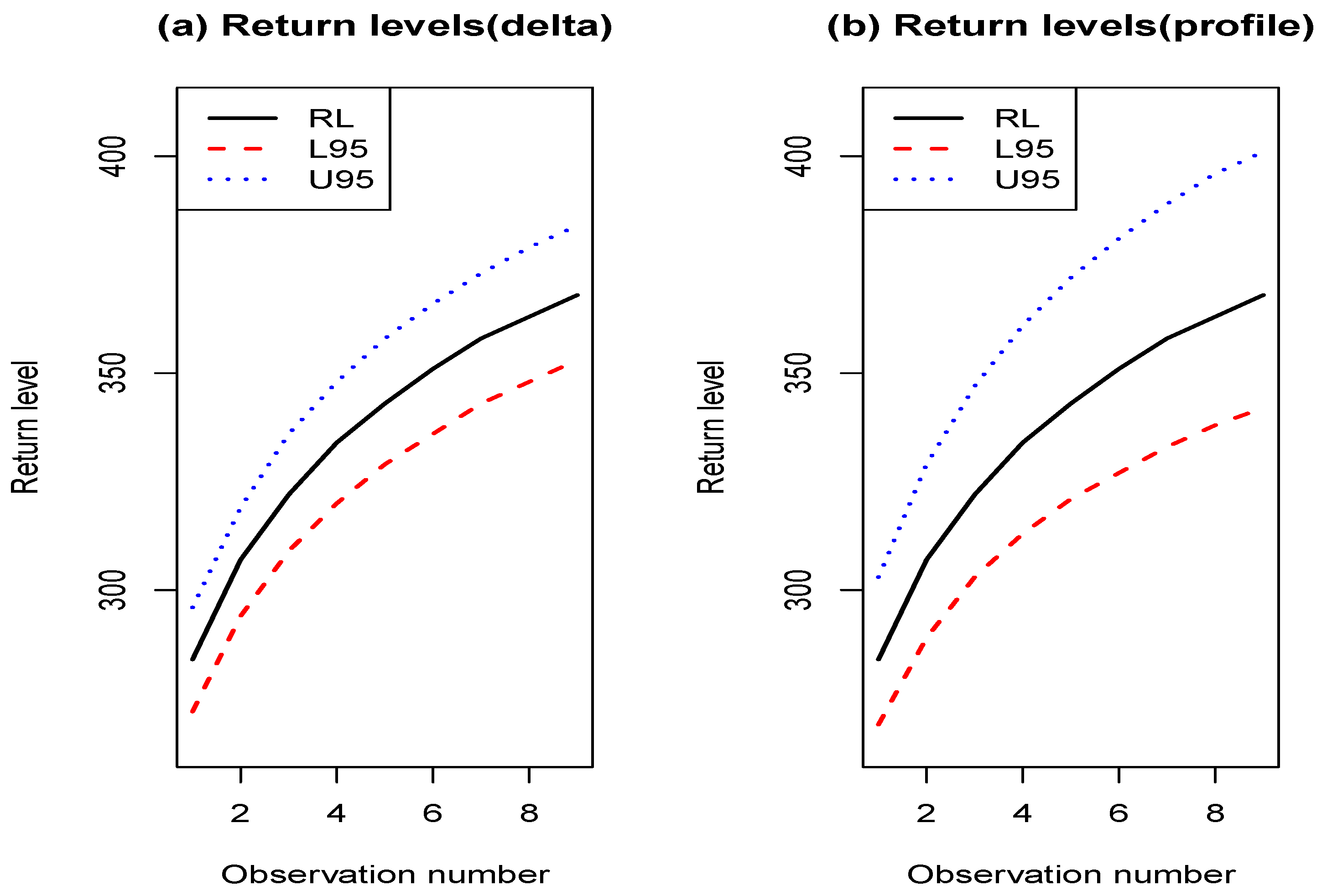
and the GPD models. The parameters of the models were estimated using the MLE method. Empirical results from the evaluation metrics for prediction intervals suggest that GEVD r = 1 , which was based on the profile likelihood, produces prediction intervals with the smallest PINAW. Modelling of extreme maximum rainfall is important in the field of hydrology for decision making. The stakeholders can be informed of return levels and periods by modelling excessive maximum rainfall in the study area, Thabazimbi. This helps in decision making and alarms the community living around Thabazimbi and surrounding areas when they are likely to experience extreme, destructive rainfall.
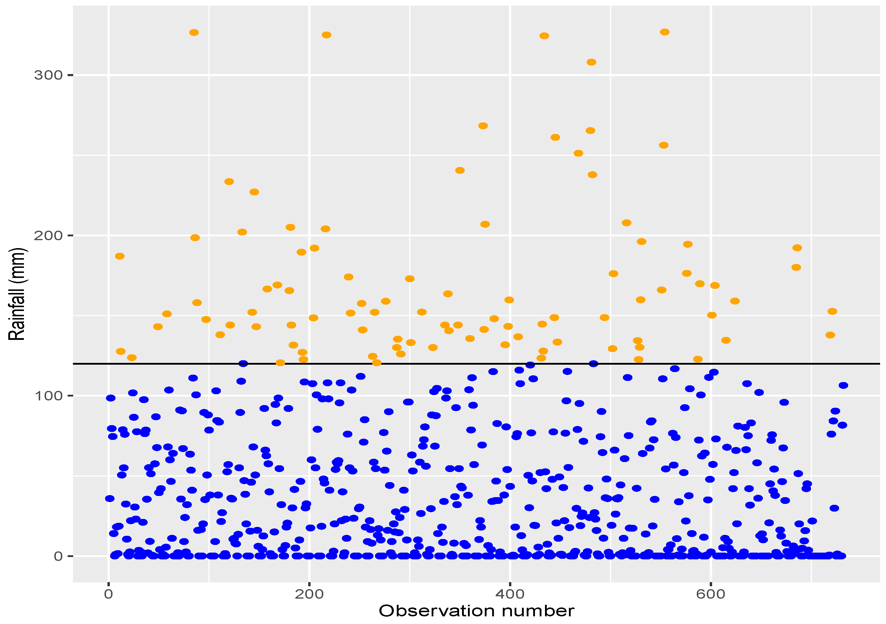
In this study, the data were tested for the existence of a monotonic trend using the Cox–Stuart (CS) trend test. Using the CS test, the p-value was 0.2492, implying no monotonic trend at the 5% level of significance. However, upon using the Mann–Kendall (MK) trend test and the seasonal MK test, we failed to reject the null hypothesis and concluded that there is both a local trend (p-value = 0.0001784) and a seasonal global trend (p-value = 0.000002689). This was then followed by computing the magnitude of the trend based on Sen’s slope test. The Weibull class of distributions is the best fitting model for the data in all the modelling frameworks. This implies that the distributions of extreme maximum rainfall are bounded above.
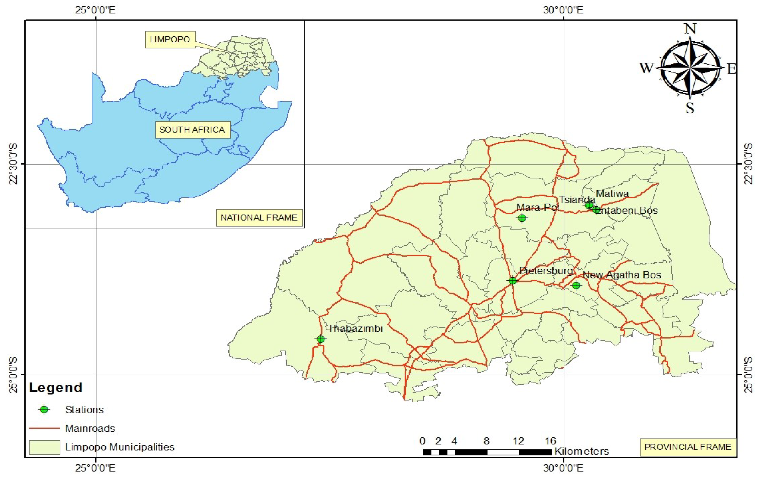
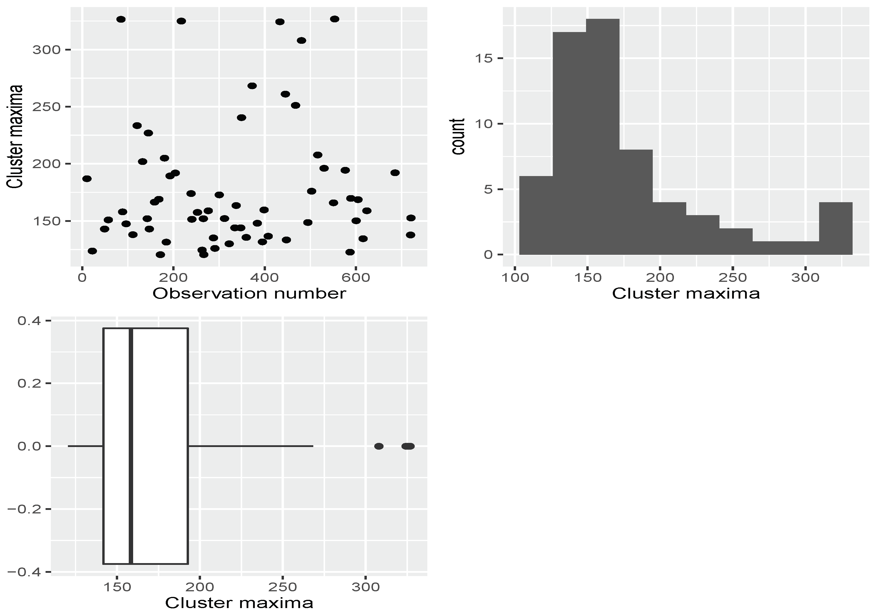
The study declustered the exceedances above a sufficiently high threshold before fitting the GPD model. It should be noted that, although the procedure of declustering and then fitting the GPD to cluster maxima gives a valid statistical model whose underlying assumptions are met, this may not be of ultimate interest in practice. For example, rainfall information can be helpful if the assessment of flood damage is the ultimate goal. Here it may be more informative to analyse complete clusters and understand the aggregate rainfall over a rainy spell rather than focus on the largest yearly value over that spell. The lack of long-term rainfall data for various stations in Limpopo province limits the other stations to be investigated in this study. The correlation between rainfall data with ocean atmospheric drivers such as SOI and IOD data was weak. As a result, these two variables were not included as covariates in the developed models in this study.
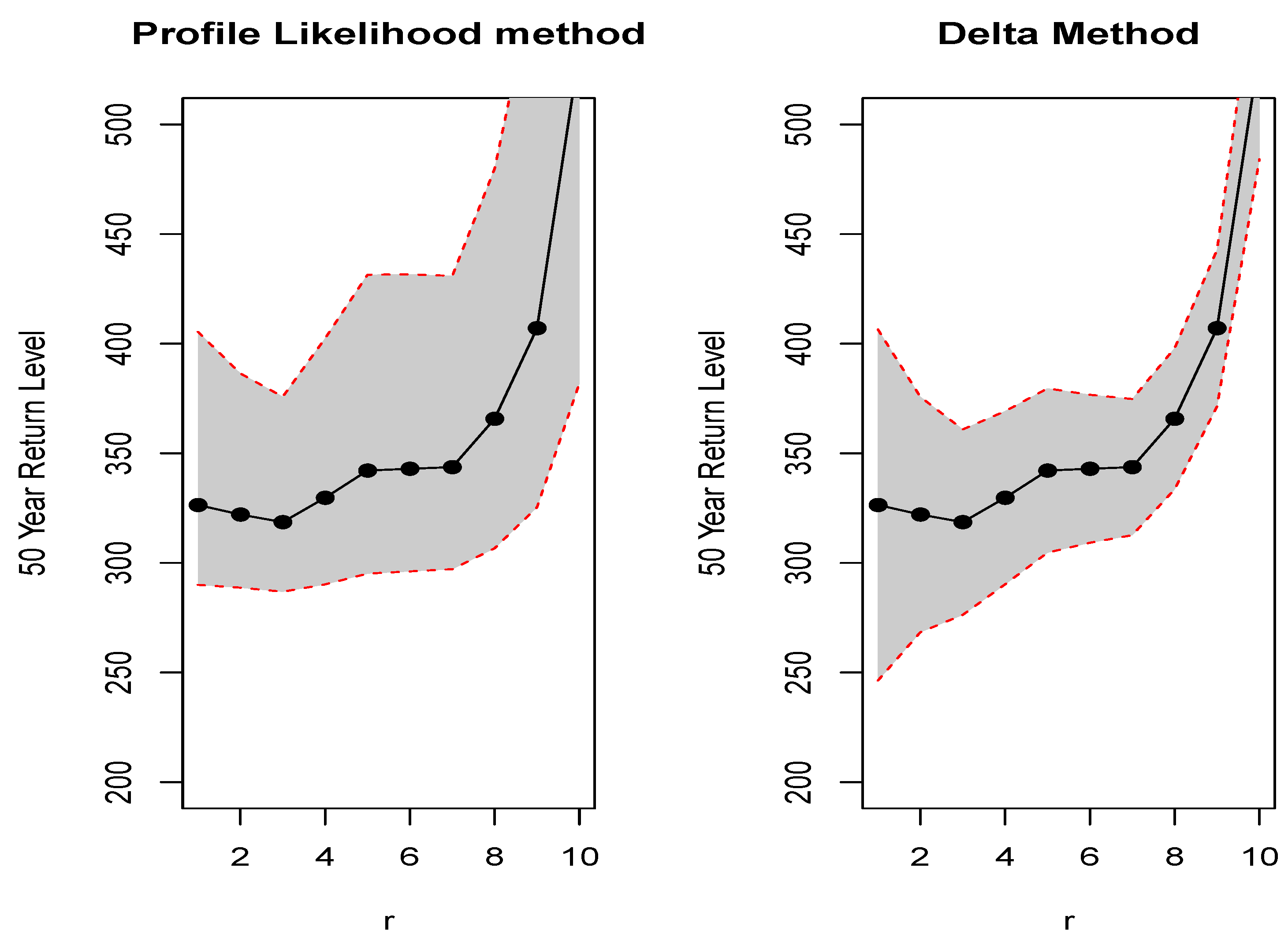
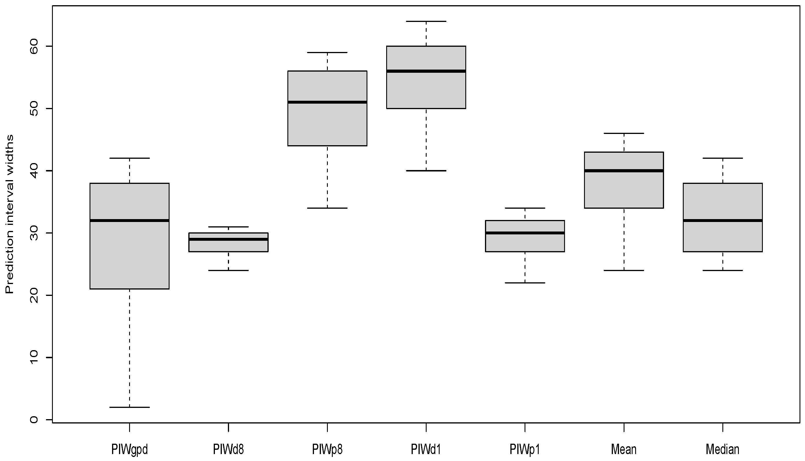
Empirical results from this study show that the prediction interval widths from the profile likelihood method are preferred to those from the delta method, as seen in Table 5. From Table 5 the delta method used on the model GEVD r = 8 has the lowest PINAW value of 1.97 from the four models: (GEVD r = 1 , delta), (GEVD r = 1 , profile), (GEVD r = 8 , delta) and (GEVD r = 8 , profile). The PINAW values from the GPD, Mean and Median models are too narrow and do not capture the uncertainty in the return levels. Robust narrower prediction intervals are preferred and usable by decision-makers in hydrology at capturing uncertainty than those too wide. Our results are consistent with those of [56] who estimated extreme flood heights using the r-largest order statistics and modelled the uncertainty in the extreme quantiles of flood heights using the delta and the profile likelihood methods, respectively. Similar studies on the use of the r-largest order statistics are given in [28,38,40,57], among others.

5. Conclusions

The paper presented the r-largest order statistics modelling approach to modelling extremely high rainfall in the Thabazimbi area in the Limpopo province of South Africa. A comparative analysis was done with the generalised Pareto distribution. The study results suggest that the data follow a GEVD and do not deviate from assumptions. Diagnostic plots for the selected station, probability plot, quantile plot, return level plot and density plot provide solid evidence that GEVD is a good fit for the block maxima data. After the suitable model for data was chosen, the 50-year return level was estimated as 368 mm, which means a probability of 0.02 exceeding 368 mm in fifty years in the Thabazimbi area. This study helps decision-makers in government and non-profit organisations improve preparation strategies and build resilience in reducing disasters resulting from extreme weather events such as excessive rainfall. Future studies may consider covariates such as the influence of ocean–atmosphere interactions on the occurrence and intensity of extremes in the Limpopo.

Author Contributions

The results of this study were obtained from a submitted masters dissertation at the University of Venda. Conceptualization, T.S. and N.N.; methodology, C.S.; software, C.S.; validation, T.S., N.N., C.S. and H.C.; formal analysis, T.S., N.N., C.S. and H.C.; investigation, T.S., N.N., C.S. and H.C.; data curation, T.S., N.N., C.S. and H.C.; writing—original draft preparation, T.S. and C.S.; writing—review and editing, T.S., N.N., C.S. and H.C.; supervision, N.N., C.S. and H.C.; project administration, N.N., C.S. and H.C. All authors have read and agreed to the published version of the manuscript.

Funding

Not applicable.

Institutional Review Board Statement

Not applicable.

Informed Consent Statement

Not applicable.

Data Availability Statement

The data used in this study are from South African Weather Services, website (https://www.weathersa.co.za/, accessed on 11 October 2021).

Acknowledgments

The authors would like to acknowledge the South African Weather Services (SAWS) for providing the data. We are also thankful to the University of Venda where this study was carried out.

Conflicts of Interest

The authors declare no conflict of interest.

Abbreviations

The following abbreviations are used in this manuscript:
CRPSContinuous Rank Probability Score
DSSDirectory of open access journals
EVTExtreme Valu Theory
GEVDGeneralised Extreme Value Distribution
GPDGeneralised Pareto Distribution
LogSLog Score
MKMann-Kendall
MLEMaximum Likelihood Estimation
POTPeaks Over Threshold
PINAWPrediction Interval Normalised Average Width
PIWPrediction Interval Width
SAWSSouth African Weather Services

References

  1. Shongwe, M.; Van Oldenborgh, G.; Van Den Hurk, B.; De Boer, B.; Coelho, C.; Van Aalst, M. Projected changes in extreme precipitation in Africa under global warming. Part 1: Southern Africa. J. Clim. 2009, 22, 3819–3837. [Google Scholar] [CrossRef]
  2. Masih, S.; Maskey, F.E.F.; Mussa and Trambauer, P. A review of droughts on the African continent: A geospatial and long-term perspective. Hydrol. Earth Syst. Sci. 2014, 18, 3635–3649. [Google Scholar] [CrossRef] [Green Version]
  3. Diriba, T.A.; Debusho, L.K. Modelling dependency effect to extreme value distributions with application to extreme wind speed at Port Elizabeth: A frequentist and Bayesian approaches. Comput. Stat. 2020, 35, 1449–1479. [Google Scholar] [CrossRef]
  4. Diriba, T.A.; Debusho, L.K.; Botai, J. Modeling extreme daily temperature using generalized Pareto distribution at Port Elizabeth. Annu. Proc. S. Afr. Stat. Assoc. Conf. (SASA) 2015, 1, 41–48. [Google Scholar]
  5. Maposa, D.; Cochran, J.J.; Lesaoana, M. Modelling extreme food heights in the lower Limpopo River basin of Mozambique using a time-heterogeneous generalised Pareto distribution. Stat. Its Interface 2017, 10, 131–144. [Google Scholar] [CrossRef]
  6. Sigauke, C.; Nemukula, M.M. Modelling extreme peak electricity demand during a heatwave period: A case study. Energy Syst. 2018, 11, 139–161. [Google Scholar] [CrossRef]
  7. Yamba, F.D.; Walimwipi, H.; Jain, S.; Zhou, P.; Cuamba, B.; Mzezewa, C. Climate change/variability implications on hydroelectricity generation in the Zambezi River Basin. mitigation and adaptation. Mitig. Adapt. Strateg. Glob. Change 2011, 16, 617–628. [Google Scholar] [CrossRef] [Green Version]
  8. Maposa, D.; Seimela, A.M.; Sigauke, C.; Cochran, J.J. Modelling temperature extremes in the Limpopo province: Bivariate time-varying threshold excess approach. Nat. Harzards 2021, 107, 2227–2246. [Google Scholar] [CrossRef] [PubMed]
  9. Gebrechorkos, S.H.; Hulsmann, S.; Bernhofer, C. Changes in temperature and precipitation extremes in Ethiopia, Kenya and Tanzania. Int. J. Climatol. 2019, 39, 18–30. [Google Scholar] [CrossRef] [Green Version]
  10. Williams, C.; Kniveton, D.; Layberry, R. Influence of South Atlantic sea surface temperatures on rainfall variability and extremes over southern Africa. J. Clim. 2008, 21, 6498–6520. [Google Scholar] [CrossRef]
  11. Layberry, R.; Kniveton, D.; Todd, M.; Kidd, C.; Bellerby, T. Daily precipitation over southern Africa: A new re-source for climate studies. J. Hydrometeor. 2006, 7, 149–159. [Google Scholar] [CrossRef] [Green Version]
  12. Reddy, C.L.; Vincent, K. Climate Risk and Vulnerability: A Handbook for Southern Africa, 2nd ed.; CSIR: Pretoria, South Africa, 2017. [Google Scholar]
  13. Hellmuth, M.; Moorhead, A.; Thomson, M.C.; Williams, J. Climate Risk Management in Africa: Learning from Practice; International Research Institute for Climate and Society, Columbia University: New York, NY, USA, 2007. [Google Scholar]
  14. Malherbe, J.; Engelbrecht, F.A.; Landman, W.A.; Engelbrecht, C.J. Tropical system from the South Indian Ocean making landfall over the Limpopo River Basin, Southern Africa: A historical perspective water. Int. J. Climatol. 2012, 32, 1018–1032. [Google Scholar] [CrossRef] [Green Version]
  15. Mdoka, M.L. Climatic Trends and Soil Moisture Feedbacks over Zimbabwe. Master’s Thesis, University of Cape Town, Cape Town, South Africa, 2005. [Google Scholar]
  16. Simonovic, S.P. Managing Water Resources: Methods and Tools for a Systems Approach; Paris and Earthscan James and James: London, UK, 2009. [Google Scholar]
  17. Edossa, D.C.; Woyessa, Y.E.; Welderufael, W.A. Analysis of droughts in the central region of South Africa and their association with SST Anomalies. Int. J. Atmos. Sci. 2014, 2014, 508953. [Google Scholar] [CrossRef] [Green Version]
  18. Krugger, A.C.; Shongwe, S. Temperature trends in South Africa: 1960–2003. Int. J. Climatol. J. R. Meteorol. Soc. 2004, 24, 1929–1945. [Google Scholar] [CrossRef]
  19. Phophi, M.M.; Mafongonya, P.; Lottering, S. Perceptions of climate change and drivers of insect pest outbreaks in vegetable crops in Limpopo province of South Africa. Climate 2020, 8, 27. [Google Scholar] [CrossRef] [Green Version]
  20. Maponya, P.; Mphandeleni, S. Climate change and agriculture production in South Africa: Impacts and adaptation options. J. Agric. Sci. 2012, 4, 48. [Google Scholar]
  21. Maposa, D.; Cochran, J.J.; Lesaoana, M.; Sigauke, C. Estimating high quantiles of extreme flood heights in the lower Limpopo River basin of Mozambique using model based Bayesian approach. Nat. Hazards Earth Syst. Sci. Discuss. 2014, 2, 5401–5425. [Google Scholar]
  22. Katz, R.W.; Parlang, M.B.; Naveau, P. Statistics of extremes in hydrology. Adv. Water Resour. 2002, 25, 1287–1304. [Google Scholar] [CrossRef] [Green Version]
  23. Embrechts, P.; Kluppelberg, C.K.I.; Mikosch, T. Modelling Extremal Events; Springer: Berlin/Heidelberg, Germany, 1997. [Google Scholar]
  24. Syafrina, A.H.; Norzaida, A.; Ain, J.J. Stationary and Nonstationary Generalized Extreme Value Models for Monthly Maximum Rainfall in Sabah. J. Phys. Conf. Ser. 2019, 1366, 012106. [Google Scholar] [CrossRef]
  25. Chifurira, R.; Chikobvu, D. Modelling extreme maximum annual rainfall for Zimbabwe. In Annual Proceedings of the South African Statistical Association Conference, Makhanda, South African, 28–30 October 2014; pp. 9–16. [Google Scholar]
  26. Nemukula, M.M.; Sigauke, C.; Maposa, D. Bivariate threshold excess models with application to extreme high temperatures in Limpopo province of South Africa. In Proceedings of the 60th Annual Conference of SASA, Johannesburg, South Africa, 26–29 November 2018; pp. 33–40. [Google Scholar]
  27. Towler, E.; Llewellyn, D.; Prein, A.; Gilleland, E. Extreme-value analysis for the characterization of extremes in water resources: A generalized workflow and case study on New Mexico monsoon precipitation. Water Clim. Extrem. 2020, 29, 100260. [Google Scholar] [CrossRef]
  28. Busababodhin, P.; Chiangpradit, M.; Papukdee, N.; Ruechairam, J.; Ruanthaisong, K.; Guayjarernpanishk, P. Extreme Value Modeling of Daily Maximum Temperature with the r-Largest Order Statistics. J. Appl. Sci. 2021, 20, 28–38. [Google Scholar] [CrossRef]
  29. Kim, H.; Kim, T.; Shin, J.-Y.; Heo, J.-H. Improvement of Extreme Value Modeling for Extreme Rainfall Using Large-Scale Climate Modes and Considering Model Uncertainty. Water 2022, 14, 478. [Google Scholar] [CrossRef]
  30. Chikobvu, D.; Sigauke, C. Modelling influence of temperature on daily peak electricity demand in South Africa. J. Energy S. Afr. 2013, 24, 63–70. [Google Scholar] [CrossRef]
  31. Mbokodo, I.L. Heat Waves in South Africa: Observed Variability Structure and Trends. Master’s Thesis, University of Venda, Thohoyandou, South Africa, 2017. [Google Scholar]
  32. Wright, C.Y.; Garland, R.M.; Norval, M.; Vogel, C. Human health impacts in a changing South African climate. S. Afr. Med. J. 2014, 104, 579–582. [Google Scholar] [CrossRef] [Green Version]
  33. Heffernan, J.E.; Tawn, J.A. A conditional approach for multivariate extreme values. J. R. Statist. Soc. B 2004, 66, 497–546. [Google Scholar] [CrossRef]
  34. Southworth, H.; Heffernan, J.E.; Metcalfe, P.D. Texmex: Statistical Modelling of Extreme Values, R Package Version 2.4.8; Available online: https://cran.r-project.org/web/packages/texmex/index.html (accessed on 5 October 2021).
  35. Minkah, R.; de Wet, T. Constant versus covariate dependent threshold in the peaks-over threshold method. J. Appl. Probab. Stat. 2014, 9, 64. [Google Scholar]
  36. Sigauke, C.; Bere, A. Modelling non-stationary time series using peaks over threshold distribution with time varying covariates and threshold: An application to peak electricity demand. Energy 2017, 119, 152–166. [Google Scholar] [CrossRef]
  37. Keef, C.; Papastathopoulos, I.; Tawn, J.A. Estimation of the conditional distribution of a multivariate variable given that one of its components is large: Additional constraints for the Hefernan and Tawn model. J. Multivar. Anal. 2013, 115, 396–404. [Google Scholar] [CrossRef]
  38. Coles, S. An Introduction to Statistical Modelling of Extreme Values; Springer: London, UK, 2001. [Google Scholar]
  39. Fisher, R.; Tippett, L. Limiting forms of the frequency distribution of the largest or smallest member of a sample. Math. Proc. Camb. Philos. Soc. 1928, 24, 180–190. [Google Scholar] [CrossRef]
  40. Bader, B.; Yan, J.; Zhang, X. Automated selection of r for the r-largest order statistics approach is done with adjustment for sequential testing. Stat. Comput. 2017, 27, 1435–1451. [Google Scholar] [CrossRef] [Green Version]
  41. Pickands, J. Statistical Inference using extreme order statistics. Ann. Stat. 1975, 3, 119–131. [Google Scholar]
  42. Heffernan, J.E.; Southworth, H. Extreme Value Modelling of Dependent Series Using R. R Vignettes: Declustering. 2020. Available online: https://github.com/janetheffernan/texmexVignettes/blob/master/declustering.pdf (accessed on 23 November 2021).
  43. Ferro, C.A.T.; Segers, J. Inference for clusters of extreme values. J. R. Stat. Soc. Ser. B (Stat. Methodol.) 2003, 65, 545–556. [Google Scholar] [CrossRef]
  44. An, Y.; Pandey, M.D. The r-largest order statistics model for extreme wind speed estimation. J. Wind. Eng. Ind. Aerodyn. 2007, 95, 165–182. [Google Scholar] [CrossRef]
  45. Bates, J.M.; Granger, C.W. The combination of forecasts. J. Oper. Res. Soc. 1969, 20, 451–468. [Google Scholar] [CrossRef]
  46. Sun, X.; Wang, Z.; Hu, J. Prediction interval construction for byproduct gas flow forecasting using optimized twin extreme learning machine. Math. Probl. Eng. 2017, 2017, 5120704. [Google Scholar] [CrossRef] [Green Version]
  47. Shen, Y.; Wang, X.; Chen, J. Wind power forecasting using multi-objective evolutionary algorithms for wavelet neural network-optimized prediction intervals. Appl. Sci. 2018, 8, 185. [Google Scholar] [CrossRef] [Green Version]
  48. Mpfumali, P.; Sigauke, C.; Bere, A.; Mulaudzi, S. Day Ahead Hourly Global Horizontal Irradiance Forecasting—Application to South African Data. Energies 2019, 12, 3569. [Google Scholar] [CrossRef] [Green Version]
  49. Mwafulirwa, N.D. Climate Variability and Predictivity in Tropical Southern Africa with a Focus on Dry Spells over Malawi. Master’s Thesis, University of Zululand, Richards Bay, South Africa, 1999. [Google Scholar]
  50. Manatsa, D.; Chingombe, H.; Matarira, C.H. The impact of the positive Indian Ocean dipole on Zimbabwe droughts. Int. J. Climatol. 2008, 28, 2011–2029. [Google Scholar] [CrossRef]
  51. Mason, S.J.; Jury, M.R. Climatic variability and change over southern Africa: A reflection on underlying processes. Prog. Phys. Geogr. 1997, 2, 23–50. [Google Scholar] [CrossRef]
  52. Marchant, R.; Mumbi, C.; Behera, S.; Yamagata, T. The Indian Ocean dipole—The unsung driver of climatic variability in East Africa. Afr. J. Ecol. 2007, 45, 4–16. [Google Scholar] [CrossRef]
  53. Mondal, A.; Mujumdar, P.P. Modeling non-stationarity in intensity, duration and frequency of extreme rainfall over India. J. Hydrol. 2015, 521, 217–231. [Google Scholar] [CrossRef]
  54. Onwuegbuche, F.; Kenyatta, A.; Affognon, S.B.; Enock, E.; Akinade, M. Application of Extreme Value Theory in Predicting Climate Change Induced Extreme Rainfall in Kenya. Int. J. Stat. Probab. 2019, 8, 85–94. [Google Scholar] [CrossRef]
  55. Nemukula, M.M.; Sigauke, C. Modelling average maximum daily temperature using r largest order statistics: An application to South African data. Jamba J. Disaster Risk Stud. 2018, 10, a467. [Google Scholar] [CrossRef] [PubMed]
  56. Robert Kajambeu, R.; Sigauke, C.; Bere, A.; Chikobvu, D.; Maposa, D.; Nemukula, M.M. Probabilistic Flood Height Estimation of the Limpopo River at the Beitbridge using r-Largest Order Statistics. Appl. Math. Inf. Sci. 2020, 14, 191–204. [Google Scholar]
  57. Smith, R.L. Extreme value theory based on the r-largest annual events. J. Hydrol. 1986, 86, 27–43. [Google Scholar] [CrossRef]
Figure 1. Flow chart of the models.
Climate 10 00033 g001
Figure 2. SAWS meteorological stations used in this study. Source: Authors’ creation.
Climate 10 00033 g002
Figure 3. Scatter plot of monthly rainfall data.
Climate 10 00033 g003
Figure 4. Return level plot using the profile likelihood and delta methods for determining best value of r = 8 .
Climate 10 00033 g004
Figure 5. Threshold stability plots. Top panel: Stability plot for the extremal index. Middle panel: Stability plot of the scale parameter. Bottom panel: Stability plot of the shape parameter.
Climate 10 00033 g005
Figure 6. Plot of exceedances.
Climate 10 00033 g006
Figure 7. Cluster maxima plots. Top left panel: Scatter plot of cluster maxima data. Top right panel: Histogram of cluster maxima data. Bottom left panel: Box plot of cluster maxima data.
Climate 10 00033 g007
Figure 8. Diagnostic plots for the stationary GPD model (M1).
Climate 10 00033 g008
Figure 9. Box plots of PIWs of the models.
Climate 10 00033 g009
Figure 10. Return level plots for the model GEVD r = 8 .
Climate 10 00033 g010
Table 1. Thabazimbi weather station information.
Station NameLatitudeLongitudeAltitude (m)Data Availability
Thabazimbi−24.617027.400010261960–2020
Table 2. Summary statistics of the monthly rainfall (MR) and annual maximum rainfall (AMR).
MinQ1Q2MeanQ3MaxStd.SkewKurt
MR002348.377.1326.860.151.653.11
AMR21.8134.3159.7172202326.866.480.6580.223
Table 3. Parameter estimates with standard errors in parentheses.
μ ^ σ ^ ξ ^
GEVD r = 1 143.6 (9.92)64 (6.91)−0.202 (0.0812)
GEVD r = 8 137.6 (10.38)66.3 (7.31)−0.103 (0.0892)
GPD 60.9 (1.21)−0.0678 (0.142)
Table 4. Summary statistics for PIW (PINC 95%).
ModelMinQ1Q2MeanQ3MaxSkewKurtStDev
GEVD r = 1 (delta)40505654.336064−0.46−1.338.08
GEVD r = 1 (profile)22273028.893234−0.33−1.514.14
GEVD r = 8 (delta)24272928.333031−0.49−1.432.55
GEVD r = 8 (profile)34445149.335659−0.46−1.368.59
GPD (MLE)2213227.63842−0.63−1.1913.8
Mean24344037.784346−0.57−1.247.51
Median24273232.3338420.13−1.806.73
Table 5. Evaluation metrics for prediction intervals.
PINC(%)ModelPINAW(%)Average PIW
95GEVD r = 1 (delta)2.2654.33
95GEVD r = 1 (profile)2.4128.89
95GEVD r = 8 (delta)1.9728.33
95GEVD r = 8 (profile)4.0549.33
95GPD (MLE)0.0727.56
95Mean0.17108.78
95Median0.22126.11
Table 6. Estimating return levels using delta and profile methods for the GEVD r = 8 model.
Delta MethodProfile Likelihood Method
Return Period (Years)(L95,RL,U95)(L95,RL,U95)Exceedance Probability
10(272,284,296)(269,284,303)0.100
15(294,307,319)(289,307,329)0.067
20(309,322,336)(303,322,347)0.050
25(320,334,348)(313,334,361)0.040
30(329,343,358)(321,343,372)0.033
35(336,351,366)(327,351,381)0.029
40(343,358,373)(333,358,389)0.025
45(348,363,379)(338,363,396)0.022
50(353,368,384)(342,368,401)0.020
Publisher’s Note: MDPI stays neutral with regard to jurisdictional claims in published maps and institutional affiliations.

