Revealing a Tipping Point in the Climate System: Application of Symbolic Analysis to the World Precipitations and Temperatures

Abstract

Climate variabilities over the period of 80 years (1930–2010) are analyzed by the combined use of divergence measures and rank correlation. First, on the basis of a statistical linguistics procedure, the m-th order differences of the monthly mean precipitations and temperatures on the globe are symbolized according to a binary coding rule. Subsequently, the annual 12-bit binary sequence for a station is divided into twelve 6-bit sequences by scanning it over a year. Computed results indicate that there is an optimal order of differences with which one can reveal the variabilities most distinctly. Specifically, it is found that for the analysis of precipitations, the second differences (m = 2) are most useful, whereas, for the temperatures, the third differences (m = 3) are preferable. A detailed comparison between the information-theoretic and the ranking methods suggests that along with the stability and coherence, owing to its ability to make an appeal to the eyes, the latter is superior to the former.

1. Introduction

In synchronism with growing concerns on climate change impacts and global warming on this planet [1,2,3], at no time has attention to climate variabilities been so arrested at present [4,5]. Climate variabilities can be appreciated through detailed analyses of time-series meteorological data such as precipitations and temperatures [6]. To date, a number of methods have been developed for detecting the onset and for revealing the symptoms of climatic anomalies arising both on the global and regional scale [7,8]. In recent years, owing to the interdisciplinary feature inherent in the time-series data analysis, various analytical tools that appear unfamiliar in conventional climatology have been applied to climatic analyses, which have been used principally in such areas as statistical physics, electrical engineering, information science, and linguistics. Of them, special novelty is seen in the detrended fluctuation analysis [9,10], a variationally optimized Markov analysis [11], Monte Carlo [12,13,14], an analysis aided by artificial neural networks [15], wavelet transformation methods [16,17], multifractal analysis [18,19,20,21], information-theoretic analysis [22,23,24,25], multiscale entropy analysis [26], statistical linguistic characterization [27,28], convergent cross mapping [29], Mahalanobis distance metrics [30], singular spectral analysis [31], the Lyapunov method [32], a method using Minkowski distance functions [33], the vectorial rotation method [34], the stochastic resonance method [35], and the generalized Zipf’s method with a scaling exponent [36].

In this paper, for 116 observational stations in the world (Figure 1), climate variabilities over the period of 80 years (1930–2010) are analyzed by the combined use of divergence measures and rank correlation. Specifically, the Kullback--Leibler divergence, Hellinger distance, and Spearman’s rank correlation are chosen. The former two are the representative information-theoretical quantities that are measured with the natural unit (nat for short), while the latter is a Pearson’s analog of the rank-ordered data and therefore is normalized and confined within [−1, 1]. Irrespective of the methods, on the basis of a statistical linguistics procedure, the m-th order differences of the monthly mean precipitations and temperatures on the globe are symbolized according to a binary coding rule. Subsequently, the annual 12-bit binary sequence for a station is divided into twelve 6-bit sequences by scanning it over a year. As a matter of fact, this procedure was initially invented for transforming time-series data into a series of discretized symbols that are processed to extract information about the generating process [37]. Of a number of successful studies on the technique [37,38,39,40,41,42,43,44,45,46], we focus our attention on the application to examining the pathological symptoms in the human heartbeat signals [43]. Here, in an effort to study climate variabilities, we attempt to apply the same methodology to revealing a climatic tipping point for our planet. This term stands for a critical point that is characterized by such adjectives as self-perpetuating, abrupt, irreversible, and perilous. Along with evidence of the points in complex networks [47,48,49,50,51,52], theoretical ecology [53], and education [54], the detection of the tipping in the climate system has been of increasing concern for sustaining contemporary societies [55,56,57,58]. At present, anxieties grow on whether this planet has already exceeded the critical point. Computed results are given for the analysis of the world precipitations and temperatures as well as the regional data in Japan. For specific orders of differences, besides the conventional first order (m = 1), both second (m = 2) and third (m = 3) differences are considered. A detailed comparison is made between the information-theoretic and the ranking methods, with which one can identify the feature of the methods.

2. Binary Coding

To explain how to generate binary sequences, we start with defining the first difference of observed values in a time-series sequence

Δx(n) ≡ x(n) − x(n − 1).

(1)

Here x(n) represents monthly mean meteorological data such as precipitations and temperatures at month n, i.e., n = 1 to n = 12, respectively, for January to December. Note that the data are averaged over thirty years [59,60,61]. Therefore, periodic conditions across the adjoining years, such as x (−1) = x (11), x (0) = x (12), and x (1) = x (13), are applicable over the thirty years of the same period. In this paper, we focus our attention on the sign of the difference, allowing us to produce the binary sequence s₁s₂…s₁₂ as [43]

s_n = 0 for Δx(n) ≤ 0; s_n = 1 for Δx(n) > 0.

(2)

As a next step, we consider the second difference

Δ²x(n) ≡ Δ(Δx(n + 1)) = x(n − 1) − 2 x(n) + x(n+1).

(3)

Here x (13) = x (1). In the coding, the same procedure as Equation (2) is adopted but replacing Δx(n) with Δ²x(n). The time series generated by the procedure corresponds to a ‘topography’ of the data. As a final step, we can produce the third difference

Δ³x(n) = Δ(Δ²x(n)) = −x(n − 2) + 3 x(n – 1) − 3 x(n) + x(n + 1).

(4)

Here x (−1) = x (11). In the coding, the same procedure as Equation (2) is adopted but replacing Δx(n) with Δ³x(n). The time series generated by the formula implies the ‘topographic variation’ of the data. To illustrate the whole procedure of the coding, an example of Edmonton (53°34′ N, 113°31′ W; h = 671 m) is shown in Figure 2. Note that finally twelve 6-bit subsequences can be obtained from a single 12-bit sequence, and thus for N stations, 12N binary symbols are generated, which are subsequently grouped into 64 categories:

#1: 000000, #2: 000001, #3: 000010, …, #63: 111110, #64: 111111.

(5)

For Period I (1930–1960) versus Period II (1950–1980), examples of the frequency and rank distributions are given in

Table 1. Example of frequency distributions for the analysis of variabilities (a) in the world precipitations (second differences) and (b) in the world temperatures (third differences).

(a)	<Period I>		<Period II>
6-Bit Code	f (Frequency)	u (Rank)	g (Frequency)	v (Rank)
#01:000000	5	61.5	1	63
#02:000001	7	57.5	1	63
#03:000010	6	60	2	61
#04:000011	12	51	5	57
#05:000100	2	64	3	59.5
#06:000101	11	53.5	13	47
#07:000110	12	51	13	47
#08:000111	15	45.5	7	54
#09:001000	3	63	7	54
#10:001001	17	38.5	9	51.5
#11:001010	27	15.5	22	28
#12:001011	26	18	25	21.5
#13:001100	16	41.5	13	47
#52:110011	25	20.5	37	5.5
#53:110100	22	29.5	17	39.5
#54:110101	31	9	37	5.5
#55:110110	23	26	35	7.5
#56:110111	23	26	22	28
#57:111000	16	41.5	13	47
#58:111001	30	11.5	33	11.5
#59:111010	26	18	20	34
#60:111011	16	41.5	26	19
#61:111100	22	29.5	23	25.5
#62:111101	17	38.5	22	28
#63:111110	15	45.5	20	34
#64:111111	16	41.6	19	37.5
(b)	<Period I>		<Period II>
6-Bit Code	f (Frequency)	u (Rank)	g (Frequency)	v (Rank)
#01:000000	11	60	16	48.5
#02:000001	25	20.5	32	9
#03:000010	27	14.5	34	4
#04:000011	32	7	32	9
#05:000100	30	9	31	12
#06:000101	23	30	33	6.5
#07:000110	17	48	19	39.5
#08:000111	35	4.5	30	14.5
#09:001000	18	45	24	26.5
#10:001001	29	11	28	18.5
#11:001010	17	48	25	23
#12:001011	29	11	34	23
#13:001100	22	34.5	15	50.5
#52:110011	15	52	38	60.5
#53:110100	20	38.5	20	35
#54:110101	24	24.5	17	45.5
#55:110110	14	54.5	10	57.5
#56:110111	4	64	4	64
#57:111000	35	4.5	46	1
#58:111001	12	58.5	11	55.5
#59:111010	28	13	5	43
#60:111011	5	63	26	63
#61:111100	24	24.5	33	6.5
#62:111101	25	20.5	6	62
#63:111110	23	30	19	39.5
#64:111111	8	61.5	8	60.5

and

Table 2. Comparison among binary code lengths for the analysis of variabilities (a) in the world precipitations (second differences) and (b) in the world temperatures (third differences).

(a) 6-Bit Coding	Period I–II		Period II–III
Kul.-Leib.: DKL (nat)	6.095 × 10−2	>	4.944 × 10−2
Hellinger: DH (nat)	2.725 × 10−2	>	2.471 × 10−2
Spearman: rS	0.8679	>	0.7873
Kendall: rK	0.6958	>	0.6250
5-bit coding	Period I–II		Period II–III
Kul.-Leib.: DKL (nat)	3.352 × 10−2	>	2.581 × 10−2
Hellinger: DH (nat)	1.478 × 10−2	>	1.302 × 10−2
Spearman: rS	0.8943	>	0.7606
Kendall: rK	0.7653	>	0.5975
4-bit coding	Period I–II		Period II–III
Kul.-Leib.: DKL (nat)	1.717 × 10−2	>	1.530 × 10−2
Hellinger: DH (nat)	7.485 × 10−3	<	7.642 × 10−3
Spearman: rS	0.9631	>	0.8215
Kendall: rK	0.8899	>	0.7187
(b) 6-bit coding	Period I–II		Period II–III
Kul.-Leib.: DKL (nat)	4.224 × 10−2	<	6.242 × 10−2
Hellinger: DH (nat)	1.976 × 10−2	<	2.985 × 10−2
Spearman: rS	0.7310	<	0.6534
Kendall: rK	0.5628	>	0.4889
5-bit coding	Period I–II		Period II–III
Kul.-Leib.: DKL (nat)	1.717 × 10−2	<	2.591 × 10−2
Hellinger: DH (nat)	8.481 × 10−3	<	1.254 × 10−2
Spearman: rS	0.7727	>	0.7524
Kendall: rK	0.6025	>	0.5449
4-bit coding	Period I–II		Period II–III
Kul.-Leib.: DKL (nat)	7.326 × 10−3	>	6.321 × 10−3
Hellinger: DH (nat)	3.641 × 10−3	>	3.165 × 10−3
Spearman: rS	0.8907	>	0.8195
Kendall: rK	0.7490	>	0.6414

, where tie data in the ranking have been dealt with according to a standard statistical procedure.

3. Analytical Methods

Climate variabilities for specific meteorological data can be analyzed in comparison between their frequency distributions across the two subsequent periods. To this end, we adopt an information-theoretic measure that is termed the Kullback--Leibler divergence [62]

D_KL (nat) = Σ p_i ln (p_i/q_i),

(6)

where p_i ≡f_i/(12N) and q_i ≡g_i/(12N) (i = 1 to 64) represent the relative frequency distributions of the periods under consideration; f_i and g_i are the frequency distributions (for details, see Table 1a,b)); the summation is made from i = 1 to 64. Note that D_KL ≥ 0 where the equality holds solely for p_i = q_i (i = 1 to 64) and that with the natural logarithm being adopted, the unit of D_KL is nat. In practical calculations, however, this measure includes a drawback, namely, for vanishing q_i, Equation (6) exhibits singularity unless p_i vanishes simultaneously. To avoid the singularity, the Hellinger distance [63] is useful:

D_H (nat) = Σ (p_i^1/2 − q_i^1/2)².

(7)

This measure that is defined in the 64-dimensional informational space can be regarded as the Euclidian analog of the Minkowski distance.

Expanding the logarithm in Equation (6) with the logarithmic series, for p_i > 0 and q_i > 0, we obtain

ln(p_i/q_i) = (p_i − q_i)/p_i + (p_i − q_i)²/(2 p_i²) + ….

(8)

The term in the right-hand side of Equation (7) can be modified through the rationalization of the numerator as

(p_i^1/2 − q_i^1/2)² = (p_i − q_i)²/(p_i^1/2 + q_i^1/2)².

(9)

Substitution of Equation (8) into Equation (6) as well as of Equation (9) into Equation (7) yields D_H→D_KL/2 as p_i→q_i for i = 1, 2, ⋯, 64.

Climate variabilities might be detected more efficiently by means of the ranking method. To this end, first, the categories (#1 to #64) are arranged into descending order according to their frequencies. For tie data to be included, a compensative technique by the median is needed. The difference of patterns between the two rankings {u} and {v} can be evaluated with the Spearman’s formula r_S = NR/DR (|r_S| ≤ 1) [64] where

NR = f (n) − (T_u’ + T_v’)/2 − 6 Σ (u_i – v_i)²,

(10)

DR = [ f (n) − T_u’ ]^1/2 [ f (n) − T_v’ ]^1/2.

(11)

Here f (n) = (n − 1) n (n + 1) = n (n² − 1) and the summation in Equation (10) is made from i = 1 to 64. The terms T_u’ and T_v’ represent contributions from the so-called rank degeneracy, which are given by T_u’ = Σ’ f (t_j) and T_v’ = Σ’ f (t_k) with the summation over the entire clusters of tie data that are included in the respective rankings.

4. Results

In what follows, numerical results are given for 116 stations on the globe (see Figure 1) as well as 75 stations in Japan; their coordinates are listed in Supplementary Material. For the world precipitations, because of the data unavailable, eight stations (Tehran, Khartoum, Djibouti, Bogota, La Paz, Lima, Maputo, and Honiara) are excluded. For both precipitations and temperatures, the entire period, 1930–2010, is segmented into Period I (1930–1960), Period II (1950–1980), and Period III (1980–2010) [59,60,61]. Note that because of an uncertain editorial reason (probably confusion and chaos across World War II), the former two periods overlap for 1951–1960; data for 1921–1950 are not available [34]. The validity of the data was detailed in [34]. From the scatter plots of rankings that are given in Figure 3, Figure 4, Figure 5, Figure 6, Figure 7 and Figure 8, we can comment as follows:

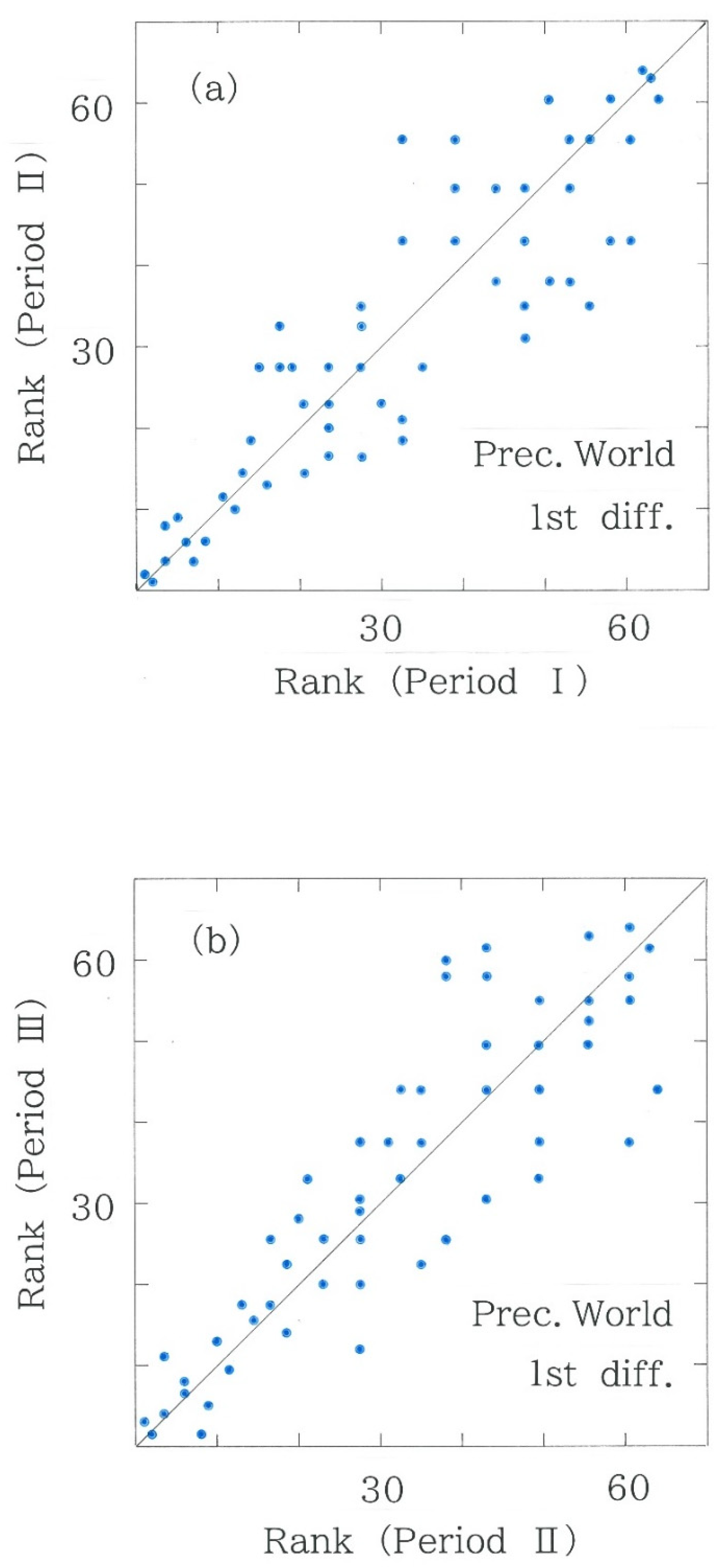
(1)

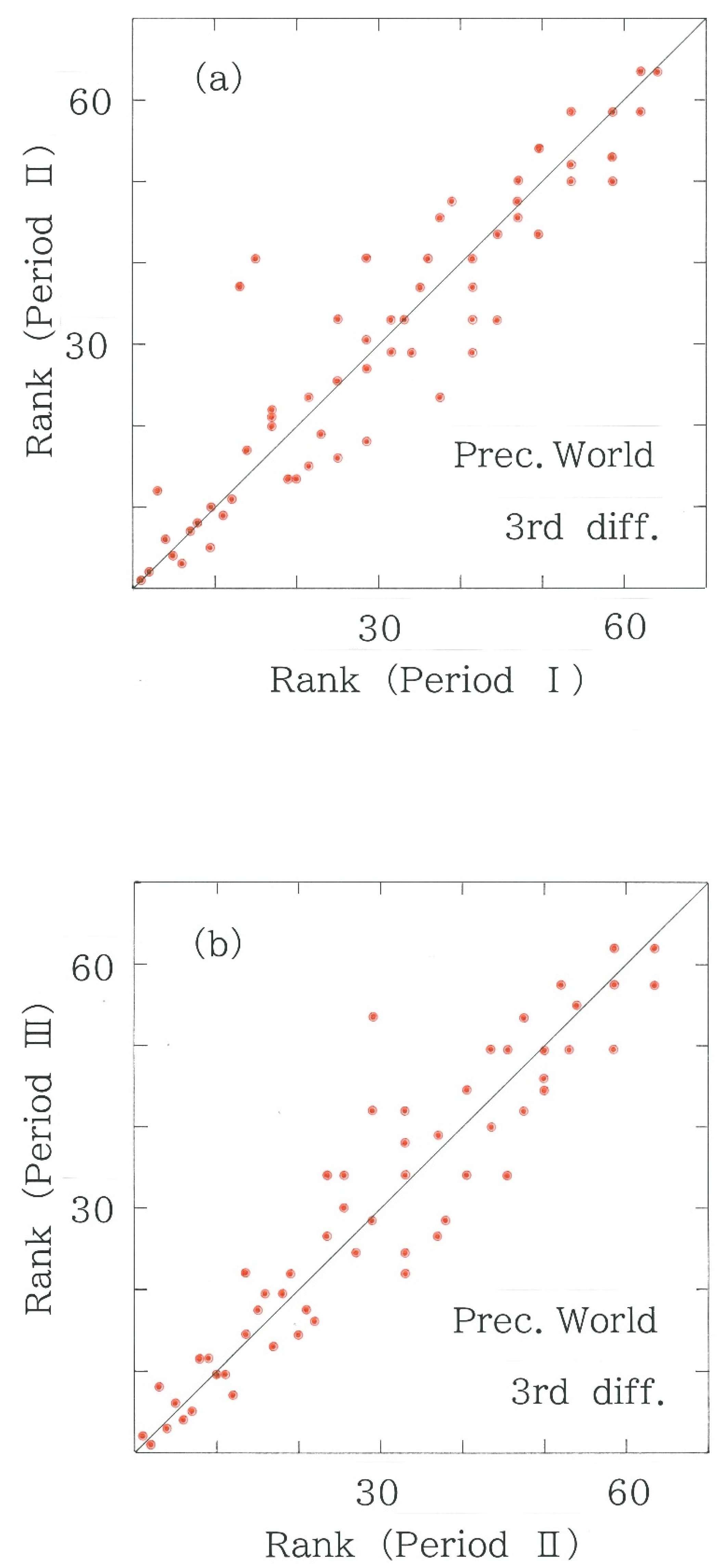
The scattergrams of the first differences in the world precipitations are shown in Figure 3a (Period II versus Period I) and in Figure 3b (Period III versus Period II). Although the 46% increase in the divergence is confirmed (i.e., D_KL = 2.24 × 10⁻² nat → 3.26 × 10⁻² nat), calculation of the Spearman’s rank correlation yields, respectively, r_S = 0.8874 and r_S = 0.8871, in which there is no significant difference. To conclude, as long as we restrict our attention to the first differences, perturbations in the world precipitations are too small to reveal significance in the climatic fluctuations.

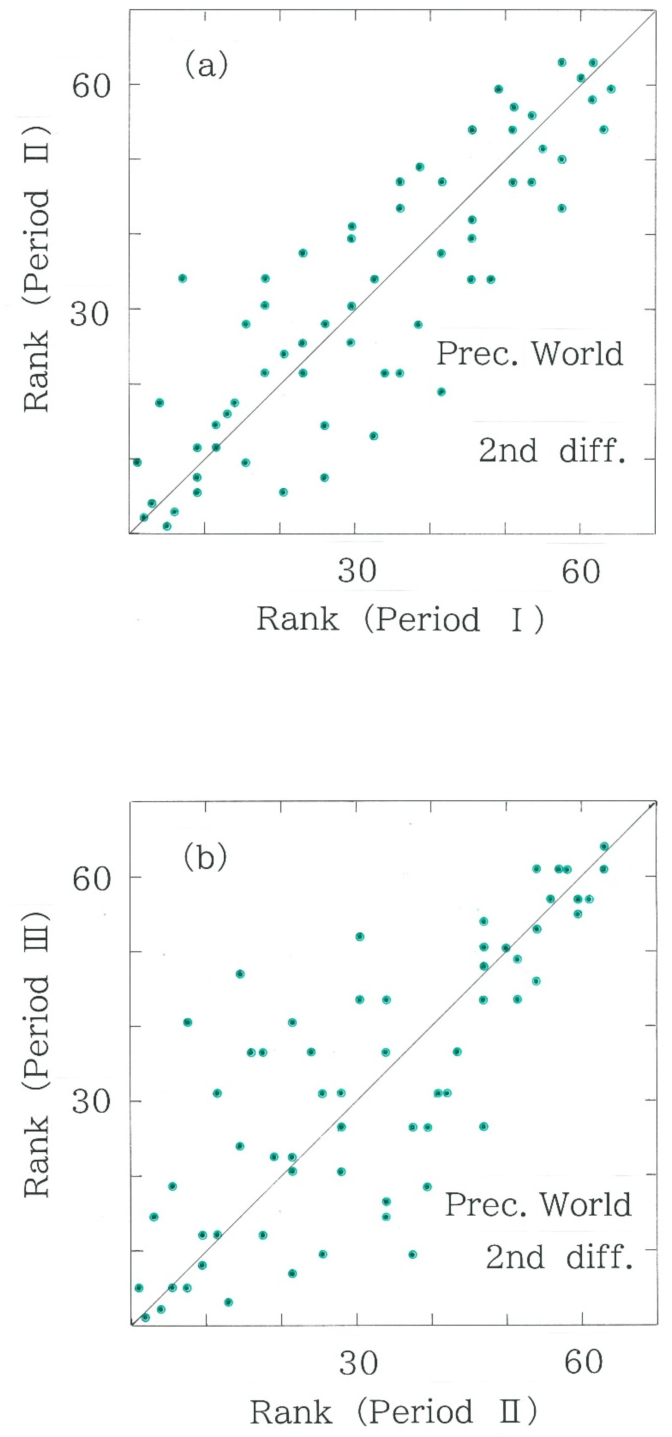
(2)

The scattergrams of the second differences in the world precipitations are shown in Figure 4a (Period II versus Period I) and in Figure 4b (Period III versus Period II). As seen in the plots, the rank correlation gets weaker in the latter (i.e., r_S = 0.8679 → 0.7873; 9.3% reduction), suggesting the enhanced variability in the precipitation data. Comparison with the divergence, however, yields the results that contradict this because the value of the latter period is smaller than the former (i.e., D_KL = 6.095 × 10⁻² nat→ 4.944 × 10⁻² nat); note that the contradiction cannot be relieved by the comparison in the Hellinger distances (D_H = 2.725 × 10⁻² nat → 2.471 × 10⁻² nat).

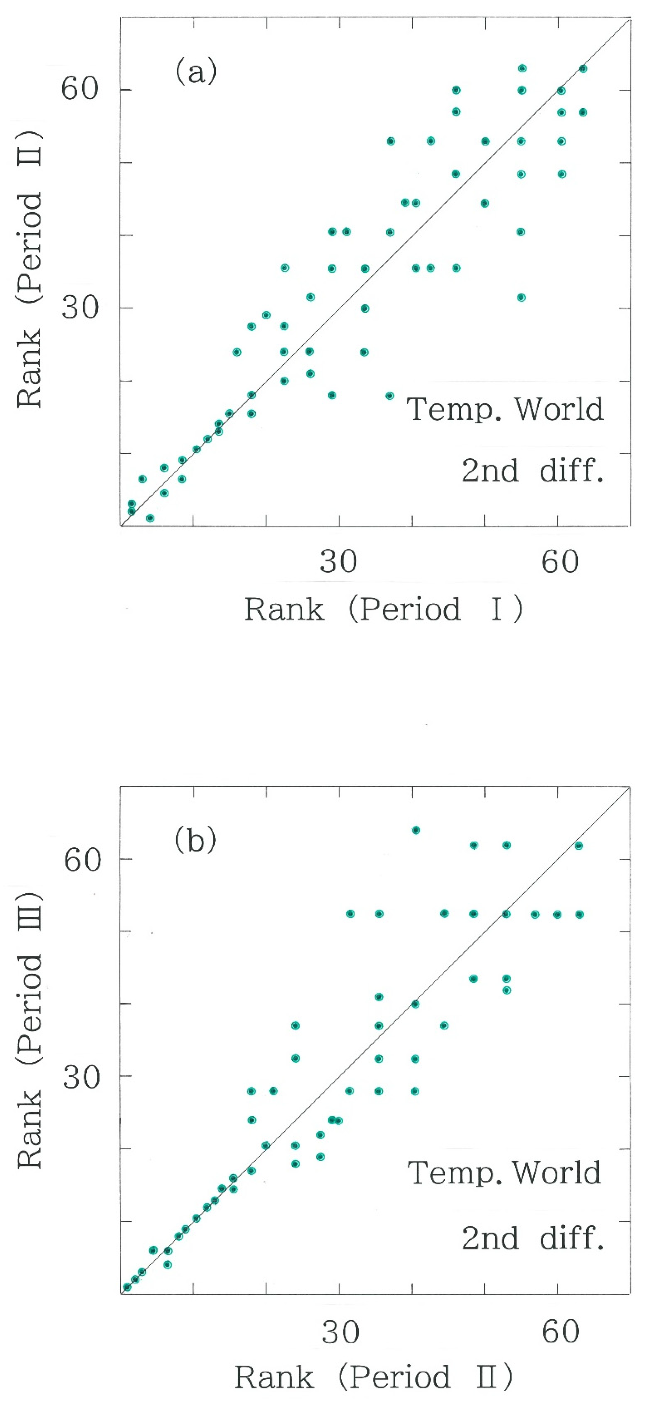
(3)

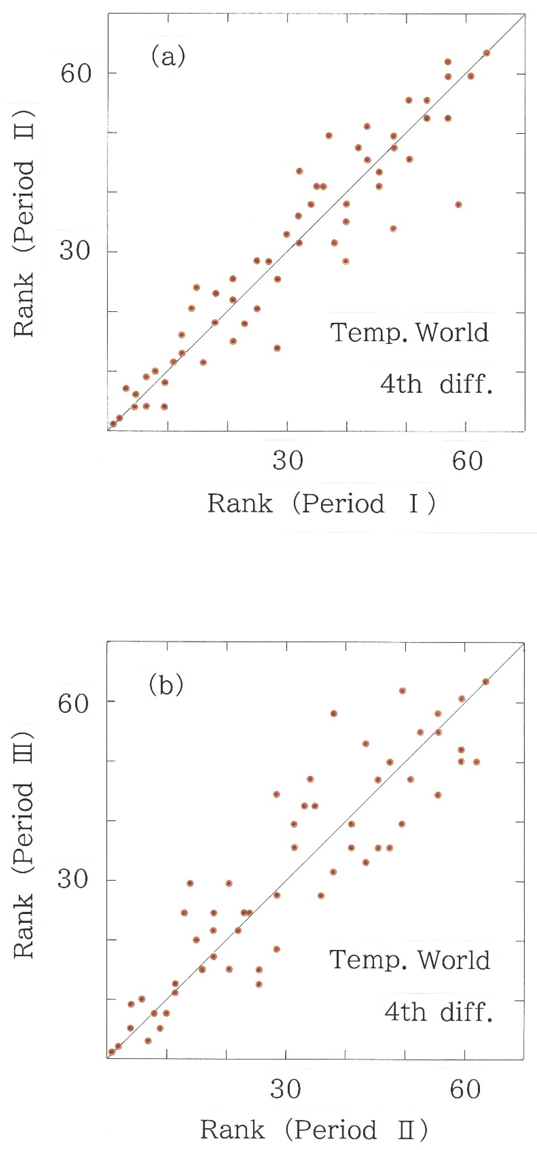
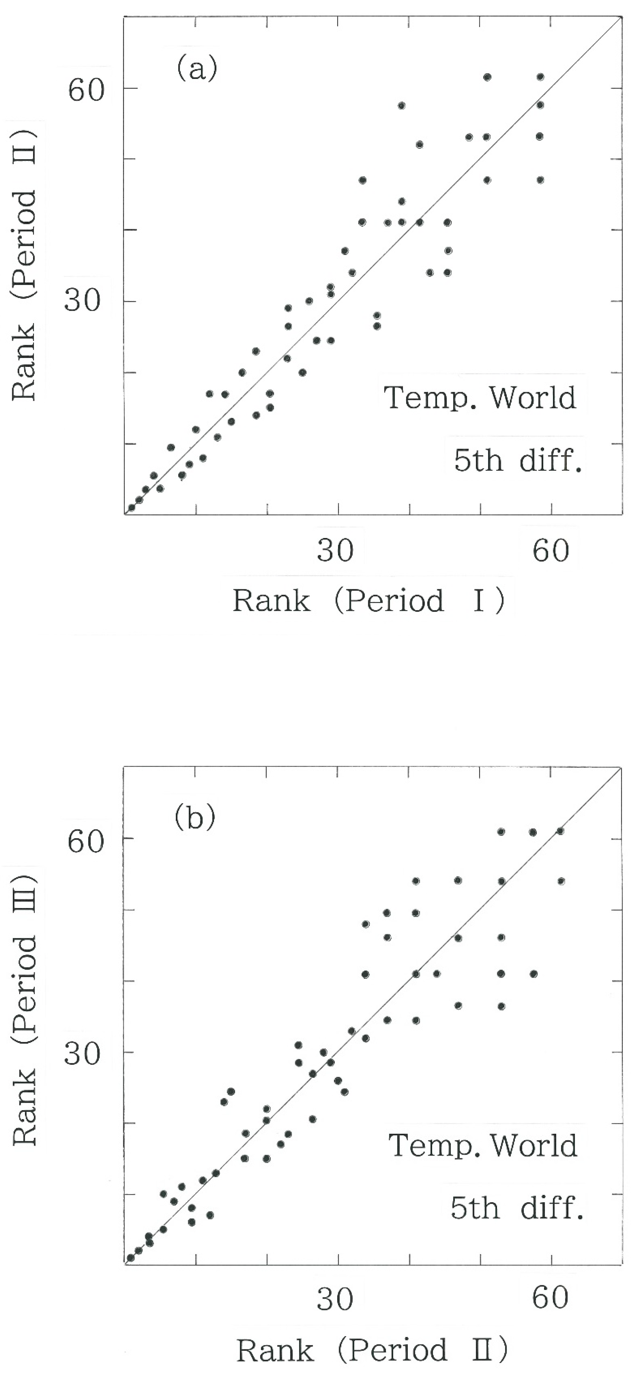
The scattergrams of the second differences in the world temperatures are shown in Figure 5a (Period II versus Period I) and in Figure 5b (Period III versus Period II). In the rank correlations (r_S = 0.9148→0.9176), as well as the Hellinger distances (D_H = 1.843 × 10⁻² nat → 1.752 × 10⁻² nat), there is no significant difference. In summary, as long as we focus our attention on the second differences, variabilities in the world temperatures are too small to reveal significance in the climatic fluctuations.

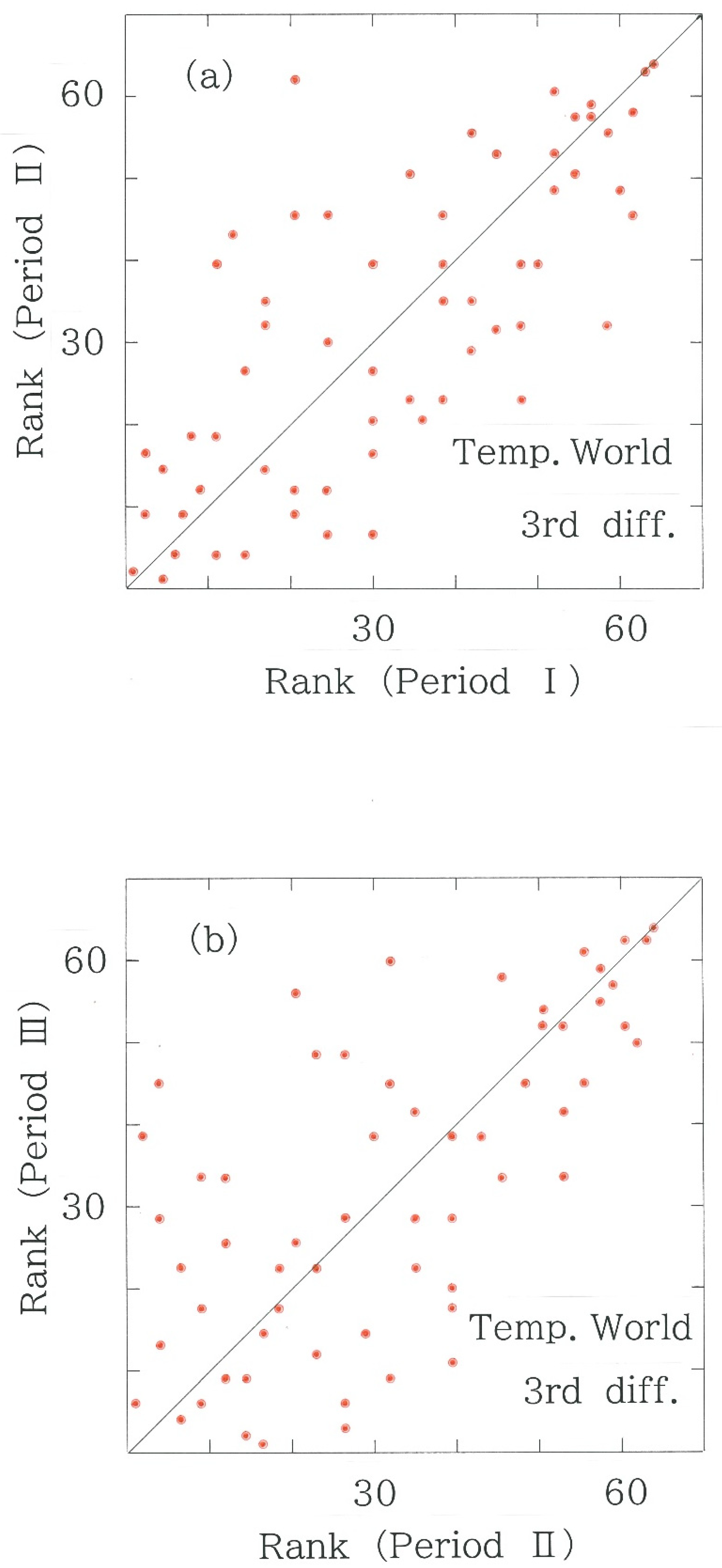
(4)

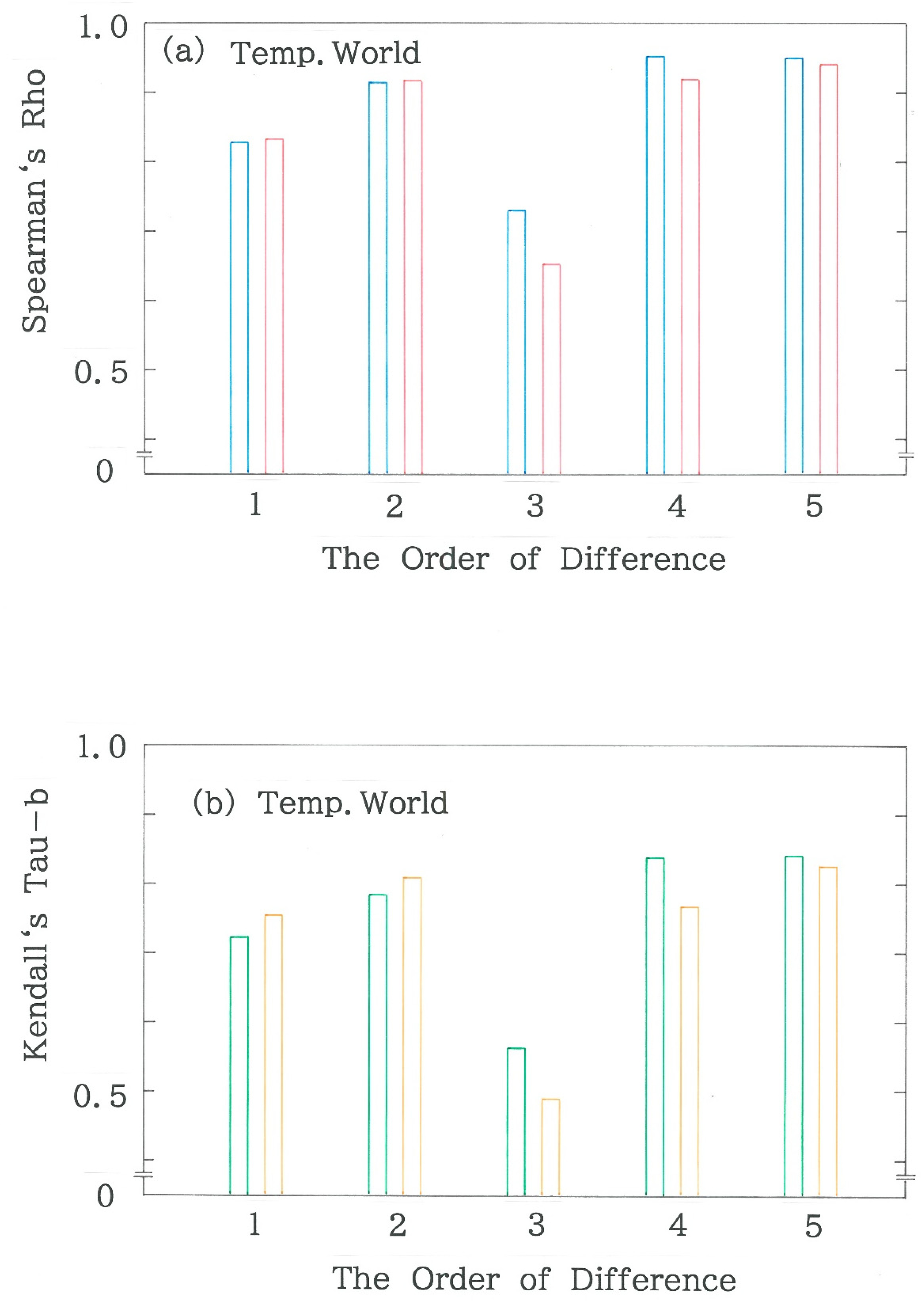
The scattergrams of the third differences in the world temperatures are shown in Figure 6a (Period II versus Period I) and in Figure 6b (Period III versus Period II). As seen in the plots, the rank correlation gets weaker in the latter (i.e., r_S = 0.7310 → 0.6534; 10.6% reduction), indicating a tipping point in the temperature data, owing to the snow/ice-albedo feedback in the regions with the higher latitudes, in particular, on the Northern Hemisphere. The effect can be explained by an increasing light absorption arising from degenerating cover of snow and ice that shows, in comparison with the seawater and the ground, relatively higher reflectivity of sunlight. In synchronism with the decrease in the correlation, both for the Kullback--Leibler divergence (D_KL = 4.224 × 10⁻² nat → 6.242 × 10⁻² nat) and for the Hellinger distance (D_H = 1.976 × 10⁻² nat→ 2.985 × 10⁻² nat), the values of the divergence measures increase considerably in the latter period. In contrast to the precipitation counterpart, for the world temperatures, one finds consistency among the three results. The results here are consistent with those obtained by our previous methods [34,36], suggesting the reliability of the present methodology.

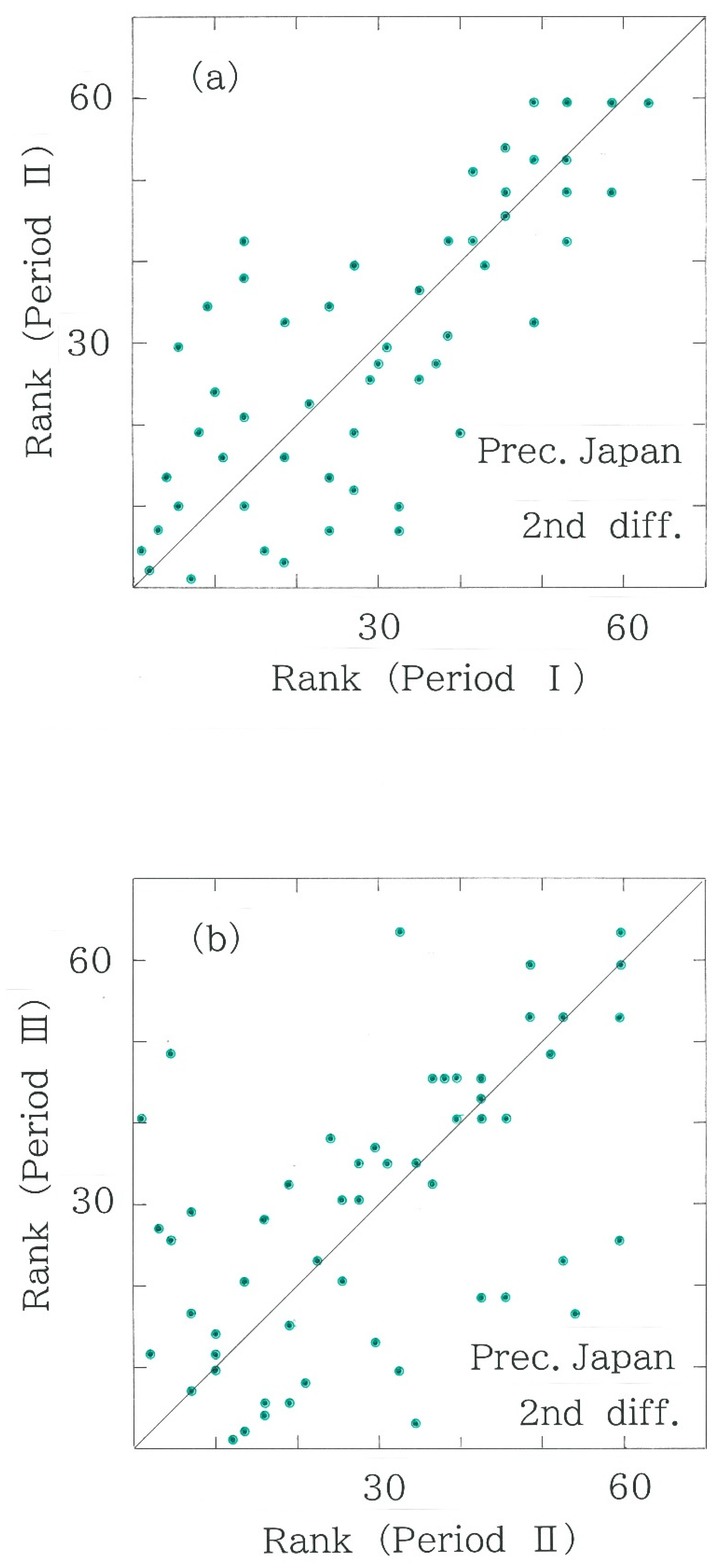
(5)

The scattergrams of the second differences in the Japanese precipitations are shown in Figure 7a (Period II versus Period I) and in Figure 7b (Period III versus Period II). As is evident in the plots, the rank correlation becomes substantially weaker in the latter (i.e., r_S = 0.8230 → 0.6547; 20.4% reduction), indicating the remarkable variability in the precipitation data. The substantial reduction larger than the above-mentioned world counterpart (9.3%) can be explained by a humid climate of the Japanese Islands. Consistent with the decrease in the rank correlation, for the Hellinger distance, the value increases substantially in the latter period (D_H = 6.991 × 10⁻² nat→ 1.617 × 10⁻¹ nat). Contrary to the world counterpart, for the domestic precipitations, we can find compatibilities in both results.

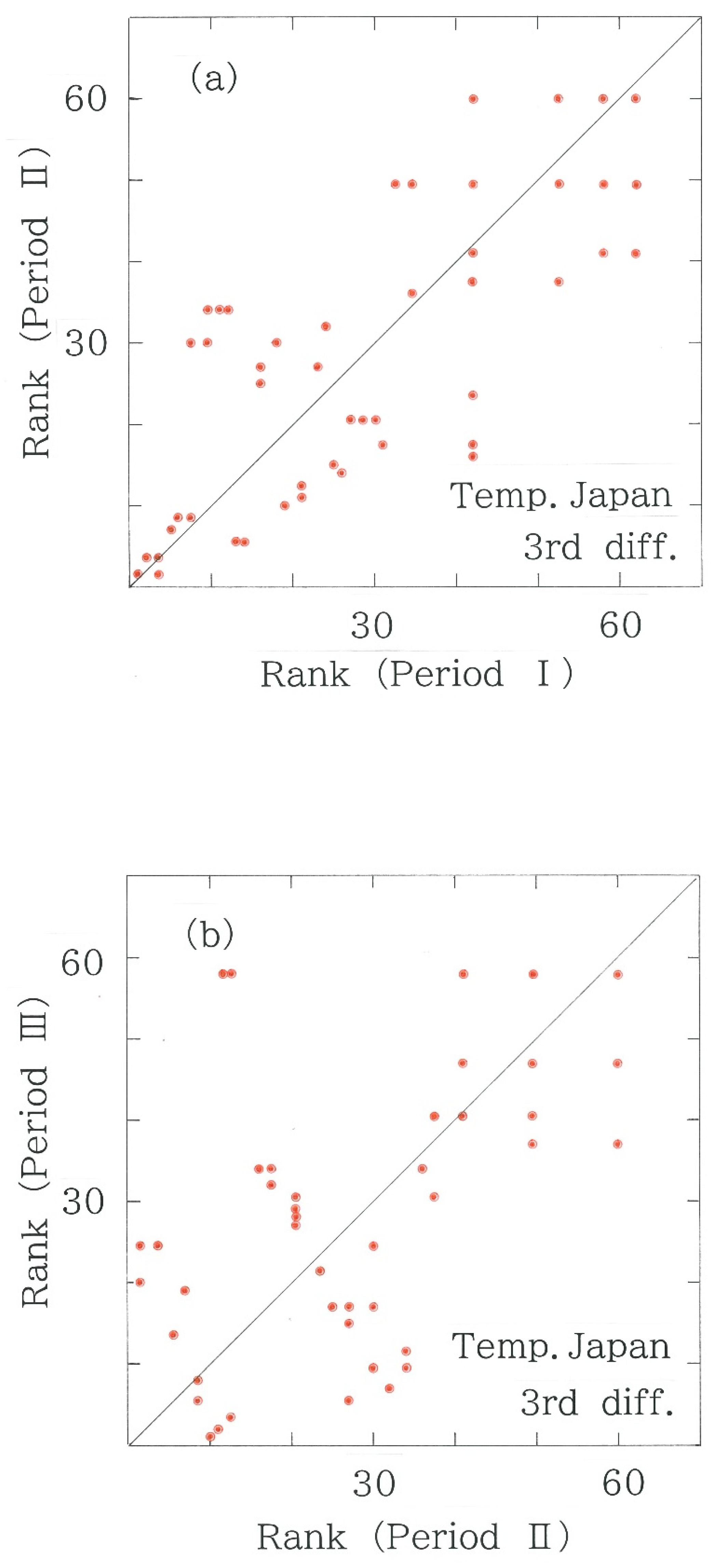
(6)

The scattergrams of the third differences in the Japanese temperatures are shown in Figure 8a (Period II versus Period I) and in Figure 8b (Period III versus Period II). In the plots, the Spearman’s correlation gets weaker in the latter (i.e., r_S = 0.7812 → 0.6910; 11.5% reduction), indicating the increasing variability and a tipping point in the temperature data. Note that the reduction is comparable to the world counterpart (10.6%) given above. In synchronism with the reduction in the rank correlation, for the Hellinger distance, the value becomes longer in the latter period (D_H = 1.646 × 10⁻¹ nat→ 2.210 × 10⁻¹ nat), indicating that consistent with the world counterpart, for the domestic temperatures as well, there is no contradiction between the two results.

5. Discussion

For the analysis of variabilities in the world precipitations, incompatibility has been seen among the results of the divergence measures and of the rank correlation. To investigate the problem in more detail, we consider other methods of coding. Computed results for 5-bit and 4-bit codes are listed in Table 2a. Instead of the 6-bit symbols shown in Figure 2, the original 12-bit binary sequence is scanned annually with the 5- or 4-bit symbols; with these modifications, Equation (5) is replaced, respectively, with

#1: 00000, #2: 00001, #3: 00010, …, #31: 11110, #32: 11111,

(12)

#1: 0000, #2: 0001, #3: 0010, …, #15: 1110, #16: 1111.

(13)

It is found from Table 2a that even if the length of symbols is changed, the incompatibility is not removed completely. In comparison with the results of the temperatures, the counterpart of Table 2a is given in Table 2b. Except for the 4-bit coding, the conclusion that has been made for the 6-bit coding is preserved. Through the results shown in Table 2a,b, it seems that because of its stability and coherence, Spearman’s ranking method (ρ) is superior to the other methods employing the divergence measures.

To confirm the above conclusion, in both tables, as an alternative type of rank correlation measure, the Kendall’s rank correlation coefficient r_K (τ_b) is also given, which is defined with the formula r_K = NR/DR (|r_K | ≤ 1) [64] where

NR = C − D,

(14)

DR = [ n (n − 1)/2 − T_u ]^1/2 [ n (n − 1)/2 − T_v ]^1/2.

(15)

Here the terms C, D, T_u, and T_v are given by the number of x_ijy_ij = 1, x_ijy_ij = −1, x_ij = 0, and y_ij = 0, respectively; x_ij and y_ij represent the so-called sign functions:

x_ij = sgn(x_i − x_j),

(16)

y_ij = sgn(y_i − y_j).

(17)

Note that sgn(t) = 1, 0, and –1, respectively, for t > 0, t = 0, and t < 0.

In the preceding section we have confirmed that, although fluctuations in the first differences of the monthly precipitations are too small to reveal effects due to the potential climate change, the fluctuations can be amplified by making use of the second differences. Here one might pose a question: could the potential variabilities in the precipitations be more highlighted with the third differences? To answer this naïve question, computed results for the third differences of the world precipitations are appended to Figure 9. Contrary to the expectation, the variations in the time series data cannot be emphasized but are reduced. Specifically, D_H = 4.619 × 10⁻² nat, and r_S = 0.9301 for Period I to II, whereas D_H = 2.355 × 10⁻² nat, and r_S = 0.9426 for Period II to III. In particular, the difference between the rank correlations is found to be too small to evaluate the significance of climate change between the two subsequent periods, indicating that there is an optimal order in the differences of time-series precipitation data.

In order to confirm that the third difference is truly optimal for revealing potential temperature variabilities, finally we consider two differences higher than three. The plots in Figure 10 and Figure 11, respectively, show the scattergrams of the fourth and fifth differences of the world temperatures; the differences are given, respectively, with

Δ⁴x(n) = Δ²(Δ²x(n)) = x(n − 2) − 4 x(n − 1) + 6 x(n) − 4 x(n + 1) + x(n + 2).

(18)

Δ⁵x(n) = Δ(Δ⁴x(n))
= −x (n − 3) + 5 x (n − 2) − 10 x (n − 1) + 10 x(n) − 5 x (n + 1) + x (n + 2).

(19)

In both figures, the differences between the rank correlations are found to be too small to evaluate the significance of the temperature change between the two subsequent periods. To conclude, in an effort to appreciate a tipping point, it has been found that there is an optimal order in the differences in time-series climatic data. In order to illustrate and highlight the finding, the order-of-difference dependence is given in Figure 12 and Figure 13. Numerical results have shown that the present methodology with the symbolization of higher-order differences may be applicable to general time-averaged measurements. For instance, there might be candidates in such areas as astronomy and geology. Incidentally, it appears that with respect to the existence of optimality, the methodology that has been discussed in this paper shares potential utilities with the principal component analysis [65], in which an optimal axis is determined by finding a multivariate configuration that yields the maximum variance of components.

6. Comparison with Other Methods

The present paper is the third one in our series of papers on climate change. Although there is no artificial data available, the reliability of the methodology can be checked solely in comparison with our previous methods [34,36]. First, it should be mentioned that the three papers deal with identical meteorological data on the 116 identical stations on the globe (Figure 1; Tables S1 and S2 in Supplementary Material) as well as 75 stations in Japan (Table S3 in Supplementary Material). Furthermore, the validity of the sampling was explained in detail in the first one [34]. For these reasons, our data can be regarded as a benchmark provided that careful comparison is made between the previous and present results. Finally, we have confirmed that besides reliable observations being reported [4,5,6], the principal results shown in Figure 4, Figure 6, Figure 7, Figure 8, Figure 12 and Figure 13, as well as Table 2a,b, are completely consistent with those given in the first [34] and second one [36]. Although, with the higher-order differences being employed, one could not immediately apply the method presented in this paper to rapidly fluctuating data without an appropriate smooth, the present time series data that are averaged over the thirty years meet the criterion. Limitations, if any, of our approach to identifying the tipping point in the system might be put on whether the point is authentic. This issue will not be resolved until the data for the forthcoming period is available.

7. Estimating Circumstances on Greenland and Antarctic

In our sampling shown in Figure 1, there are stations neither on Greenland nor on Antarctica where complete data over the three periods are not available [59,60,61]. For the former two periods (Period I and II), however, data are available for three Greenlandic stations [59,60],

• Egedesminde (68°42′ N, 52°45′ W; h = 47 m),
• Angmagssalik (65°36′ N, 37°38′ W; h = 52 m), and
• Prins Christian Sund (60°02′ N, 43°07′ W; h = 19 m),

while for the last period (Period III), data are available solely for the capital [61],

• Nuuk (64°10′ N, 51°45′ W; h = 80 m),

besides the ones for two base stations in Antarctica [61], namely,

• Vostok (78°27′ S, 106°52′ E; h = 3488 m; from Russia) and
• Showa (69°00′ S, 39°35′ E; h = 18 m; from Japan).

With the temperature data across Period I and II being available, the rotation angle θ [34,36] from the former (Period I) to the latter (Period II) can be computed as

• θ = 2.65° for Egedesminde,
• θ = 9.74° for Angmagssalik, and
• θ = 4.05° for Prins Christian Sund.

One can find that among the 116 world stations, the angle above is placed on rank 17, 2, and 4, respectively [36], suggesting that circumstances in Greenland are comparable to or possibly more severe than the Nordic countries [66,67,68].

As mentioned above, in contrast to Greenland, the data available for Antarctica are very limited. For this reason, one can make no estimation but comparing the 12-bit binary sequences between Ushuaia (54°48′ S, 68°19′ W; h = 28 m) on the southernmost spot of the South American continent (plotted in Figure 1) and the two Antarctic stations. For the third differences in the temperatures, we obtain

• 001111010011 for Ushuaia,
• 111110110000 for Showa, and
• 011000011000 for Vostok.

The results allow one to calculate the Hamming distance H (0 ≤ H ≤ 12) between two binary sequences:

• H = 6 between Ushuaia and Showa,
• H = 7 between Ushuaia and Vostok, and
• H = 5 between Showa and Vostok.

With these results in mind, we can see at least a correlation between the Hamming distance and the geographic one, suggesting again that along with Greenland, circumstances in Antarctica are perilous [69,70,71,72].

8. Conclusions

Climate variabilities over the period of 80 years (1930–2010) have been analyzed by the combined use of divergence measures and rank correlation. With a statistical linguistics approach, the m-th order differences of the monthly mean precipitations and temperatures on the globe have been symbolized according to a binary coding rule. Subsequently, the 12-bit binary sequence for a station has been segmented into twelve 6-bit sequences. Numerical results have shown that for the analysis of precipitations, the second differences (m = 2) are most useful, whereas, for the temperatures, the use of the third differences (m = 3) is preferable. Quantitative comparison between the information-theoretic and the ranking methods has suggested that on account of its visualization, stability, and coherence, the latter is superior to the former. Furthermore, it has been confirmed that the conclusion on the accelerating climate variabilities is consistent with those of the previous reports [4,5,6]. On the basis of this speculation, continuous efforts must be made to examine how the climate variabilities on this planet grow toward the forthcoming period (Period IV: 2010–2040). Furthermore, at the beginning of the next century, data over six periods (Period I to VI) are available, which will allow one to make the comparative analysis not only for the period of thirty years but also of sixty years (i.e., instead of division as Period I, II, III, IV, V, and VI, division as Period I/II, III/IV, and V/VI is possible).

References

- Weart, S.R. The Discovery of Global Warming; Harvard University Press: Cambridge, MA, USA, 2008. [Google Scholar]
- Berger, J.J. Climate Peril; Northbrae: Berkeley, CA, USA, 2014. [Google Scholar]
- Wadhams, P. A Farewell to Ice: A Report from the Arctic; Penguin Books: London, UK, 2016. [Google Scholar]
- HadCRUT4 Dataset Produced by the Met Office and the Climatic Research Unit at the University of East Anglia; Global Climate in Context as the World Approaches 1 °C above Pre-Industrial for the First Time. 2015. Available online: https://www.metoffice.gov.uk/research/news/2015/global-average-temperature-2015 (accessed on 19 July 2020).
- GOSAT Project, the National Institute for Environmental Studies, Japan. A Prompt Report on the Monthly Mean Carbon-Dioxide Concentration Averaged over the Entire Atmosphere. 2016. Available online: http://www.gosat.nies.go.jp/recent-global-co2.html (accessed on 19 July 2020).
- Stocker, T.F.; Qin, D.; Plattner, G.-K.; Tignor, M.M.B.; Allen, S.K.; Boschung, J.; Nauels, A.; Xia, Y.; Bex, V.; Midgley, P.M. (Eds.) Climate Change 2013: The Physical Science Basis (Working Group I Contribution to the Fifth Assessment Report of the Intergovernmental Panel on Climate Change); Cambridge University Press: Cambridge, UK, 2014. [Google Scholar]
- von Storch, H.; Zwiers, F.W. Statistical Analysis in Climate Research; Cambridge University Press: Cambridge, UK, 2000. [Google Scholar]
- von Storch, H.; Navarra, A. (Eds.) Analysis of Climate Variability: Applications of Statistical Techniques, 2nd ed.; Springer: Berlin, Germany, 2010. [Google Scholar]
- Király, A.; Jánosi, I.M. Stochastic modeling of daily temperature fluctuations. Phys. Rev. E 2002, 65, 051102. [Google Scholar] [CrossRef] [PubMed]
- Yu, D.-L.; Li, W.J.; Zhou, Y. Analysis of trends in air temperature at Chinese stations considering the long-range correlation effect. Phys. A 2019, 533, 122034. [Google Scholar] [CrossRef]
- Lind, P.G.; Mora, A.; Gallas, J.A.C.; Haase, M. Reducing stochasticity in the North Atlantic Oscillation index with coupled Langevin equations. Phys. Rev. E 2005, 72, 056706. [Google Scholar] [CrossRef] [PubMed]
- Redner, S.; Petersen, M.R. Role of global warming on the statistics of record-breaking temperatures. Phys. Rev. E 2006, 74, 061114. [Google Scholar] [CrossRef]
- Newman, W.I.; Malamud, B.D.; Turcotte, D.L. Statistical properties of record-breaking temperatures. Phys. Rev. E 2010, 82, 066111. [Google Scholar] [CrossRef]
- Tamazian, A.; Ludescher, J.; Bunde, A. Significance of trends in long-term correlated records. Phys Rev E 2015, 91, 032806. [Google Scholar] [CrossRef]
- Verdes, P.F. Global warming is driven by anthropogenic emissions: A time series analysis approach. Phys. Rev. Lett. 2007, 99, 048501. [Google Scholar] [CrossRef]
- Rossi, A.; Massei, N.; Laignel, B. A synthesis of the time-scale variability of commonly used climate indices using continuous wavelet transform. Glob. Planet. Chang. 2011, 78, 1–13. [Google Scholar] [CrossRef]
- Zhang, F.; Yang, P.; Fraedrich, K.; Zhou, X.; Wang, G. Reconstruction of driving forces from nonstationary time series including stationary regions and application to climate change. Phys. A 2017, 473, 337–343. [Google Scholar] [CrossRef]
- Kim, S.Y.; Lim, G.; Chang, K.-H.; Jung, J.W.; Kim, K.; Park, C.H. Multifractal analysis of rainfalls in Korean Peninsula. J. Korean Phys. Soc. 2008, 52, 669. [Google Scholar] [CrossRef]
- Millán, H.; Kalauzi, A.; Cukic, M.; Biondi, R. Nonlinear dynamics of meteorological variables: Multifractality and chaotic invariants in daily records from Pastaza, Ecuador. Theor. Appl. Clim. 2010, 102, 75–85. [Google Scholar] [CrossRef]
- Moon, W.; Agarwal, S.; Wettlaufer, J.S. Intrinsic pink-noise multidecadal global climate dynamics mode. Phys. Rev. Lett. 2018, 121, 108701. [Google Scholar] [CrossRef]
- da Silva, H.S.; Silva, J.R.S.; Stosic, T. Multifractal analysis of air temperature in Brazil. Phys. A 2020, 549, 124333. [Google Scholar] [CrossRef]
- Saco, P.M.; Carpi, L.C.; Figliola, A.; Serrano, E.; Rosso, O.A. Entropy analysis of the dynamics of El Niño/Southern oscillation during the Holocene. Phys. A 2010, 389, 5022–5027. [Google Scholar] [CrossRef]
- Balasis, G.; Donner, R.V.; Potirakis, S.M.; Runge, J.; Papadimitriou, C.; Daglis, I.A.; Eftaxias, K.; Kurths, J. Statistical mechanics and information-theoretic perspectives on complexity in the earth system. Entropy 2013, 15, 4844–4888. [Google Scholar] [CrossRef]
- Garland, J.; Jones, T.R.; Neuder, M.; White, J.W.C.; Bradley, E. An information-theoretic approach to extracting climate signals from deep polar ice cores. Chaos 2019, 29, 101105. [Google Scholar] [CrossRef]
- Ikuyajolu, O.J.; Falasca, F.; Bracco, A. Information entropy as quantifier of potential predictability in the tropical Indo-Pacific basin. Front. Clim. 2021, 3, 675840. [Google Scholar] [CrossRef]
- Balzter, H.; Tate, N.J.; Kaduk, J.; Harper, D.; Page, S.; Morrison, R.; Muskulus, M.; Jones, P. Multi-scale entropy analysis as a method for time-series analysis of climate data. Climate 2015, 3, 227–240. [Google Scholar] [CrossRef]
- Primo, C.; Galván, A.; Sordo, C.; Gutiérrez, J.M. Statistical linguistic characterization of variability in observed and synthetic daily precipitation series. Phys. A 2007, 374, 389–402. [Google Scholar] [CrossRef]
- Vindel, J.M.; Polo, J. Markov processes and Zipf’s law in daily solar irradiation at earth’s surface. J. Atmos. Sol.-Terrestr. Phys. 2014, 107, 42–47. [Google Scholar] [CrossRef]
- Huang, X.; Hassani, H.; Ghodsi, M.; Mukherjee, Z.; Gupta, R. Do trend extraction approaches affect causality detection in climate change studies? Phys. A 2017, 469, 604–624. [Google Scholar] [CrossRef][Green Version]
- Matcharashvili, T.; Zhukova, N.; Chelidze, T.; Founda, D.; Gerasopoulos, E. Analysis of long-term variation of the annual number of warmer and colder days using Mahalanobis distance metrics: A case study for Athens. Phys. A 2017, 487, 22–31. [Google Scholar] [CrossRef]
- Hassani, H.; Silva, E.S.; Gupta, R.; Das, S. Predicting global temperature anomaly: A definitive investigation using an ensemble of twelve competing forecasting models. Phys. A 2018, 509, 121–139. [Google Scholar] [CrossRef]
- Wang, C.; Wang, Z.H.; Li, Q. Emergence of urban clustering among U.S. cities under environmental stressors. Sustain. Cities Soc. 2020, 63, 102481. [Google Scholar] [CrossRef]
- Wang, C.; Wang, Z.H.; Sun, L. Early-warning signals for critical temperature transitions. Geophys. Res. Lett. 2020, 47, e2020GL088503. [Google Scholar] [CrossRef]
- Hayata, K. Global-scale synchronization in the meteorological data: A vectorial analysis that includes higher-order differences. Climate 2020, 8, 128. [Google Scholar] [CrossRef]
- Das, M.; Kantz, H. Stochastic resonance and hysteresis in climate with state-dependent fluctuations. Phys. Rev. E 2020, 101, 062145. [Google Scholar] [CrossRef] [PubMed]
- Hayata, K. An attempt to appreciate climate change impacts from a rank-size rule perspective. Front. Phys. 2022, 9, 687900. [Google Scholar] [CrossRef]
- Daw, C.S.; Finney, C.E.A.; Tracy, E.R. A review of symbolic analysis of experimental data. Rev. Sci. Instr. 2003, 74, 915–930. [Google Scholar] [CrossRef]
- Hsu, A.T.; Marshall, A.G.; Ricca, T.L. Clipped representations of Fourier-transform ion-cyclotron resonance mass spectra. Anal. Chim. Acta 1985, 178, 27–41. [Google Scholar] [CrossRef]
- Hao, B. Symbolic dynamics and characterization of complexity. Phys. D 1991, 51, 161–176. [Google Scholar] [CrossRef]
- Dolnik, M.; Bollt, E.M. Communication with chemical chaos in the presence of noise. Chaos 1998, 8, 702–710. [Google Scholar] [CrossRef][Green Version]
- Godelle, J.; Letellier, C. Symbolic sequence statistical analysis for free liquid jets. Phys. Rev. E 2000, 62, 7973. [Google Scholar] [CrossRef] [PubMed]
- Bandt, C.; Pompe, B. Permutation entropy: A natural complexity measure for time series. Phys. Rev. Lett. 2002, 88, 174102. [Google Scholar] [CrossRef] [PubMed]
- Yang, A.C.-C.; Hseu, S.S.; Yien, H.W.; Goldberger, A.L.; Peng, C.-K. Linguistic analysis of the human heartbeat using frequency and rank order statistics. Phys. Rev. Lett. 2003, 90, 108103. [Google Scholar] [CrossRef] [PubMed]
- Zunino, L.; Soriano, M.C.; Rosso, O.A. Distinguishing chaotic and stochastic dynamics from time series by using a multiscale symbolic approach. Phys. Rev. E 2012, 86, 046210. [Google Scholar] [CrossRef]
- Pisarchik, A.N.; Huerta-Cuellar, G.; Kulp, C.W. Statistical analysis of symbolic dynamics in weakly coupled chaotic oscillators. Commun. Nonlinear Sci. Numer. Simulat. 2018, 62, 134–145. [Google Scholar] [CrossRef]
- Ma, Y.; Hou, F.; Yang, A.C.; Ahn, A.C.; Fan, L.; Peng, C.-K. Symbolic dynamics of electroencephalography is associated with the sleep depth and overall sleep quality in healthy adults. Phys. A 2019, 513, 22–31. [Google Scholar] [CrossRef]
- Zhang, W.; Lim, C.; Szymanski, B.K. Analytic treatment of tipping points for social consensus in large random networks. Phys. Rev. E 2012, 86, 061134. [Google Scholar] [CrossRef]
- Doyle, C.; Sreenivasan, S.; Szymanski, B.K.; Korniss, G. Social consensus and tipping points with opinion inertia. Phys. A 2016, 443, 316–323. [Google Scholar] [CrossRef]
- Doyle, C.; Szymanski, B.K.; Korniss. Effects of communication burstiness on consensus formation and tipping points in social dynamics. Phys. Rev. E 2017, 95, 062303. [Google Scholar] [CrossRef] [PubMed]
- Peng, X.; Zhao, Y.; Small, M. Identification and prediction of bifurcation tipping points using complex networks based on quasi-isotropic mapping. Phys. A 2020, 560, 125108. [Google Scholar] [CrossRef]
- Donovan, G.M.; Brand, C. Spatial early warning signals for tipping points using dynamic mode decomposition. Phys. A 2022, 596, 127152. [Google Scholar] [CrossRef]
- Moghadam, N.N.; Ramamoorthy; Nazarimehr, F.; Rajagopal, K.; Jafari, S. Tipping points of a complex network biomass model: Local and global parameter variations. Phys. A 2022, 592, 126845. [Google Scholar] [CrossRef]
- Meng, Y.; Jiang, J.; Grebogi, C.; Lai, Y.C. Noise-enabled species recovery in the aftermath of a tipping point. Phys. Rev. E 2020, 101, 012206. [Google Scholar] [CrossRef]
- Jayman, M.; Glazzard, J.; Rose, A. Tipping point: The staff wellbeing crisis in higher education. Front. Educ. 2022, 7, 590. [Google Scholar] [CrossRef]
- Pierini, S. Stochastic tipping points in climate dynamics. Phys. Rev. E 2012, 85, 027101. [Google Scholar] [CrossRef]
- Bentley, R.A.; Maddison, E.J.; Ranner, P.H.; Bissell, J.; Caiado, C.C.S.; Bhatanacharoen, P.; Clark, T.; Botha, M.; Akinbami, F.; Hollow, M.; et al. Social tipping points and earth systems dynamics. Front. Environ. Sci. 2014, 2, 35. [Google Scholar] [CrossRef]
- Corner, S.; Jones, C. Tipping points: Climate surprises. Front. Young Minds 2021, 9, 703610. [Google Scholar] [CrossRef]
- Blaustein, R. Warning signs of tipping point for Greenland ice sheet. Physics 2021, 14, 80. [Google Scholar] [CrossRef]
- The National Astronomical Observatory, Japan (Ed.) Chronological Scientific Tables; Maruzen: Tokyo, Japan, 1985; Volume 59, pp. 196–365. [Google Scholar]
- The National Astronomical Observatory, Japan (Ed.) Chronological Scientific Tables; Maruzen: Tokyo, Japan, 1992; Volume 66, pp. 196–365. [Google Scholar]
- The National Astronomical Observatory, Japan (Ed.) Chronological Scientific Tables; Maruzen: Tokyo, Japan, 2017; Volume 91, pp. 184–319. [Google Scholar]
- Kullback, S. Information Theory and Statistics; Dover: New York, NY, USA, 1997; pp. 6–7. [Google Scholar]
- Pardo, L. (Ed.) New Developments in Statistical Information Theory Based on Entropy and Divergence Measures; MDPI AG: Lausanne, Switzerland, 2019; p. 51. [Google Scholar]
- Conover, W.J. Practical Nonparametric Statistics, 3rd ed.; Wiley: New York, NY, USA, 1999; pp. 314–321. [Google Scholar]
- Jolliffe, I.T. Principal Component Analysis, 2nd ed.; Springer: Berlin, Germany, 2002. [Google Scholar]
- Broeke, M.V.D.; Box, J.; Fettweis, X.; Hanna, E.; Noël, B.; Tedesco, M.; van As, D.; van de Berg, W.J.; van Kampenhout, L. Greenland ice sheet surface mass loss: Recent developments in observation and modeling. Curr. Clim. Chang. Rep. 2017, 3, 345–356. [Google Scholar] [CrossRef]
- Trusel, L.D.; Das, S.B.; Osman, M.B.; Evans, M.J.; Smith, B.E.; Fettweis, X.; McConnell, J.R.; Noël, B.P.Y.; Broeke, M.R.V.D. Nonlinear rise in Greenland runoff in response to post-industrial Arctic warming. Nature 2018, 564, 104–108. [Google Scholar] [CrossRef]
- Pattyn, F.; Ritz, C.; Hanna, E.; Asay-Davis, X.; DeConto, R.; Durand, G.; Favier, L.; Fettweis, X.; Goelzer, H.; Golledge, N.R.; et al. The Greenland and Antarctic ice sheets under 1.5°C global warming. Nat. Clim. Chang. 2018, 8, 1053–1061. [Google Scholar] [CrossRef]
- Thackeray, C.W.; Fletcher, C.G. Snow albedo feedback: Current knowledge, importance, outstanding issues and future directions. Prog. Phys. Geogr. Earth Environ. 2016, 40, 392–408. [Google Scholar] [CrossRef]
- Scambos, T.A.; Hulbe, C.; Fahnestock, M.; Bohlander, J. The link between climate warming and break-up of ice shelves in the Antarctic Peninsula. J. Glaciol. 2017, 46, 516–530. [Google Scholar] [CrossRef]
- Clem, K.R.; Fogt, R.L.; Turner, J.; Lintner, B.R.; Marshall, G.J.; Miller, J.R.; Renwick, J.A. Record warming at the South Pole during the past three decades. Nat. Clim. Chang. 2020, 10, 762–770. [Google Scholar] [CrossRef]
- Cordero, R.R.; Sepúlveda, E.; Feron, S.; Damiani, A.; Fernandoy, F.; Neshyba, S.; Rowe, P.M.; Asencio, V.; Carrasco, J.; Alfonso, J.A.; et al. Black carbon footprint of human presence in Antarctica. Nat. Commun. 2022, 13, 984. [Google Scholar] [CrossRef]