

Climate Change Effects upon Pasture in the Alps: The Case of Valtellina Valley, Italy


Abstract
1. Introduction
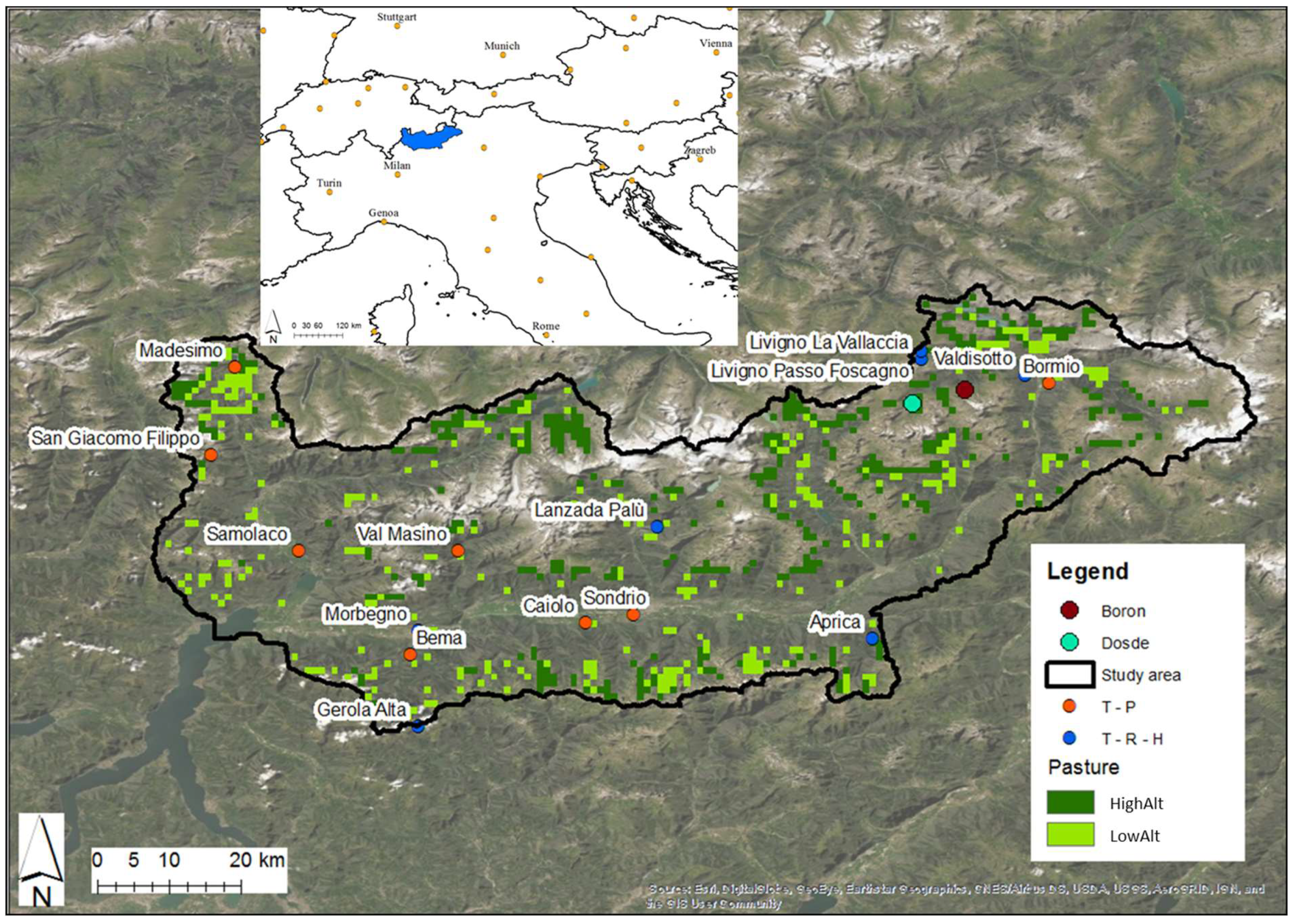
2. Case Study Area
3. Data and Methods
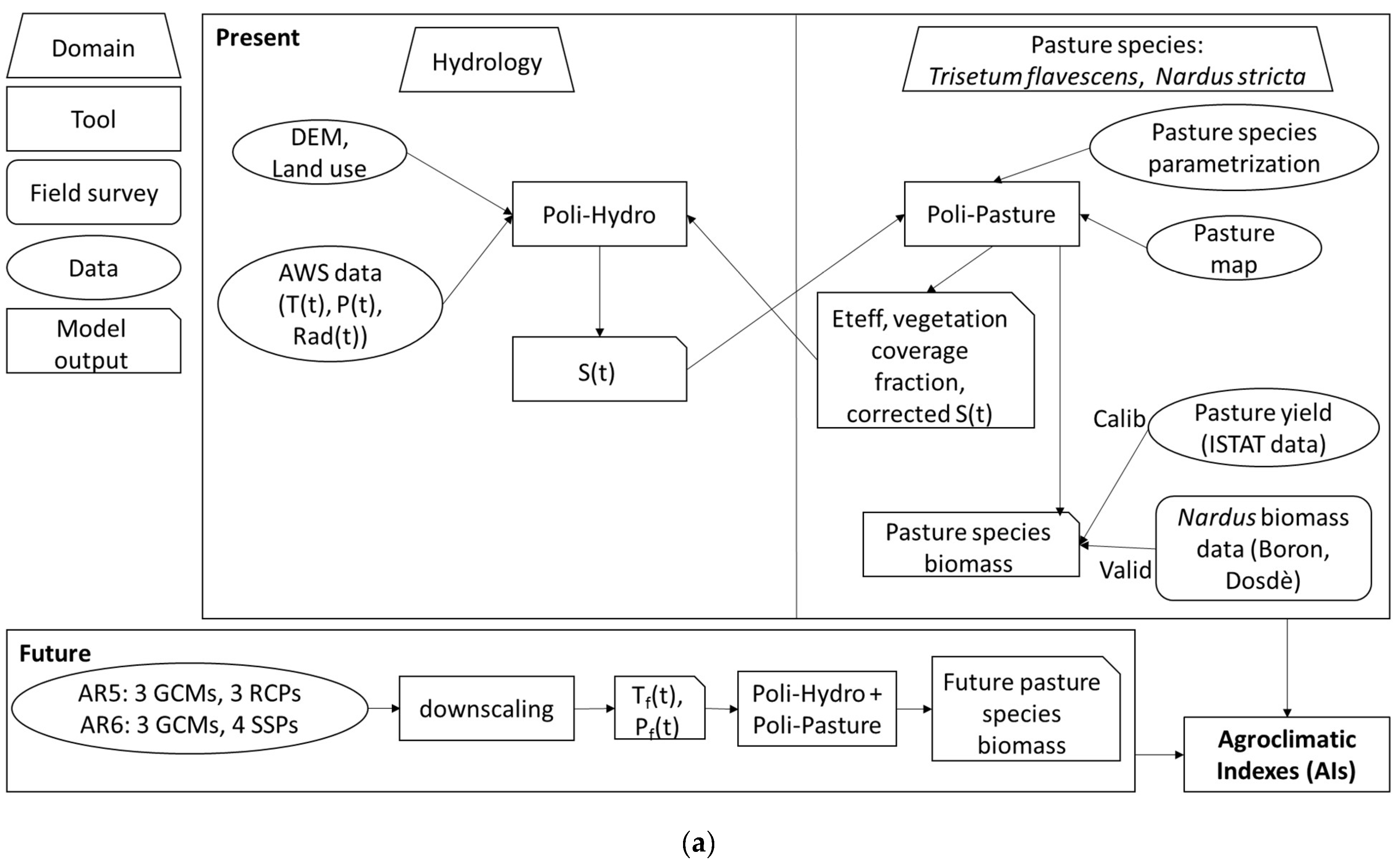
3.1. Hydrological and Pasture Model
3.2. Weather Data
3.3. Land Cover and Soil Properties
3.4. Pasture Productivity
3.5. Climate Projections and Future Simulations
3.6. Agroclimatic Indices
4. Results
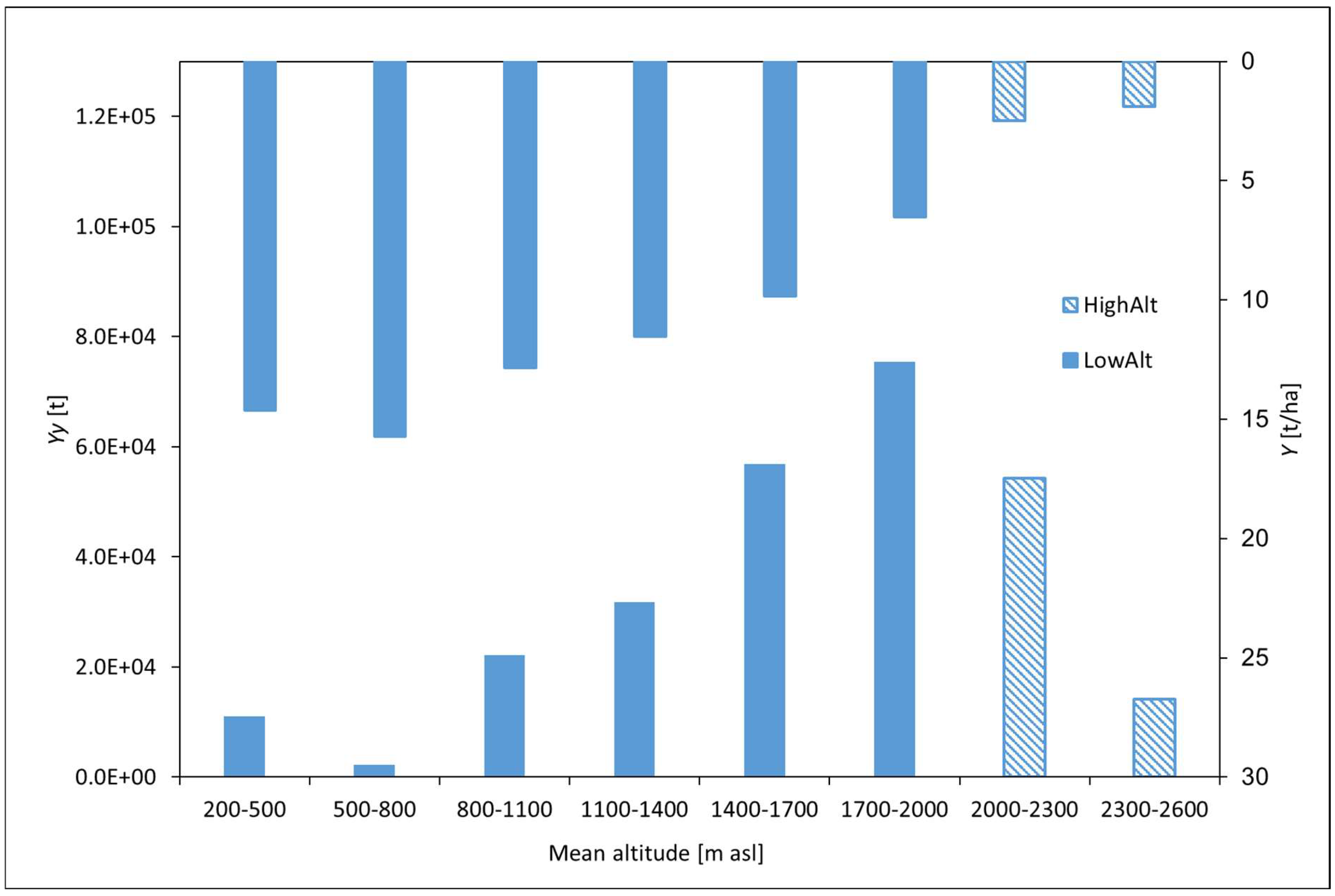
4.1. Pasture Species Productivity in the Present Period (2003–2019)
4.1.1. Calibration of the Model Using ISTAT Data in the CR Period (2006–2017)
4.1.2. Validation of the Model Using In Situ Data (2003, 2004, 2019)
4.1.3. Uncertainties in Calibration Data
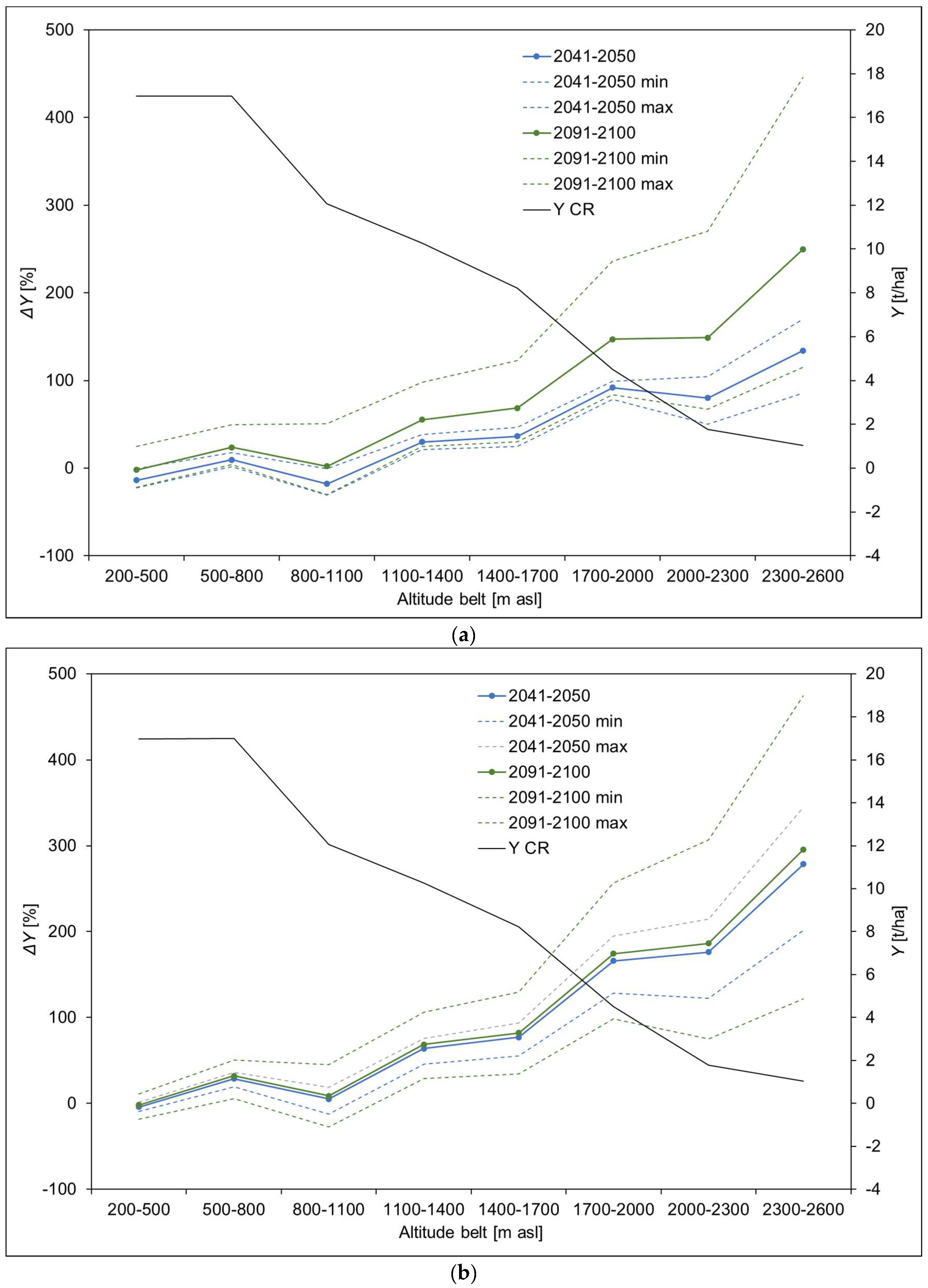
4.2. Future Pasture Species Productivity
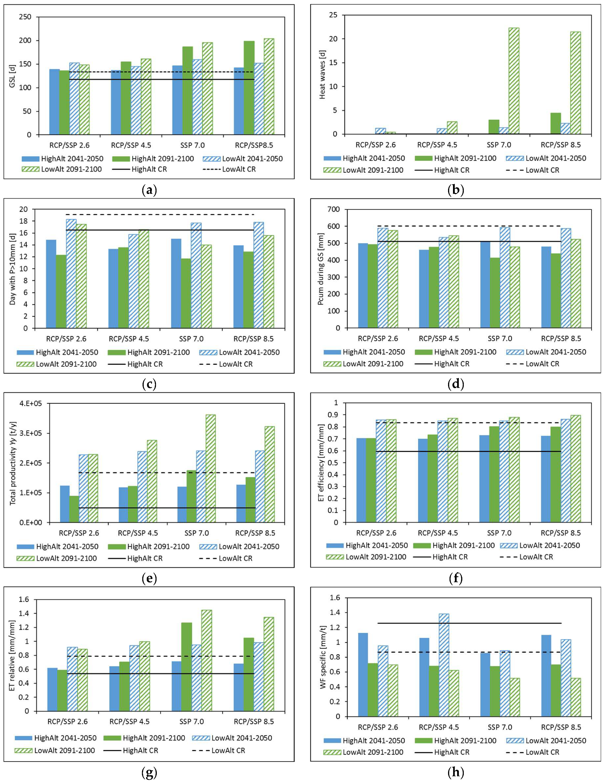
4.3. Agroclimatic Indices
5. Discussion
5.1. The Calibration of Poli-Hydro+Poli-Pasture Model
5.2. Projections of Potential Changes in Pasture Dynamic and Productivity
5.3. Choice of Two Index Pasture Species
5.4. Limitations and Future Improvements of the Simulation
6. Conclusions
Author Contributions
Funding
Data Availability Statement
Acknowledgments
Conflicts of Interest
Appendix A. Poli-Hydro and Poli-Pasture Models
Appendix A.1. Poli-Hydro Model
Appendix A.2. Poli-Pasture Model
References
- Mazzocchi, C.; Ruggeri, G.; Sali, G. The role of tourists for pastures resilience and agriculture sustainability in the Alps: A multivariate analysis approach. In Proceedings of the 7th AIEAA Conference Evidence-based Policies to Face New Challenges for Agri-Food Systems, Conegliano, Italy, 14–15 June 2018. [Google Scholar]
- Faccioni, G.; Sturaro, E.; Ramanzin, M.; Bernués, A. Socio-economic valuation of abandonment and intensification of Alpine agroecosystems and associated ecosystem services. Land Use Policy 2019, 81, 453–462. [Google Scholar] [CrossRef]
- Hock, R.; Rasul, G.; Adler, C.; Cáceres, B.; Gruber, S.; Hirabayashi, Y.; Jackson, M.; Kääb, A.; Kang, S.; Kutuzov, S.; et al. Chapter 2: High Mountain Areas. IPCC Special Report on the Ocean and Cryosphere in a Changing Climate. IPCC Spec. Rep. Ocean. Cryosphere A Chang. Clim. 2019, 131–202. [Google Scholar]
- Böhm, R.; Auer, I.; Brunetti, M.; Maugeri, M.; Nanni, T.; Schöner, W. Regional temperature variability in the European Alps: 1760–1998 from homogenized instrumental time series. Int. J. Climatol. 2001, 21, 1779–1801. [Google Scholar] [CrossRef]
- Brunetti, M.; Lentini, G.; Maugeri, M.; Nanni, T.; Simolo, C.; Spinoni, J. 1961–1990 high-resolution Northern and Central Italy monthly precipitation climatologies. Adv. Sci. Res. 2009, 3, 73–78. [Google Scholar] [CrossRef]
- Dettinger, M.D.; Cayan, D.R. Large-scale atmospheric forcing of recent trends towards early snowmelt runoff in California. J. Clim. 1995, 606–623. [Google Scholar] [CrossRef]
- Cayan, D.R. Interannual climate variability and snowpack in the western United States. J. Clim. 1996, 928–948. [Google Scholar] [CrossRef]
- Haeberli, W.; Beniston, M. Climate change and its impacts on glaciers and permafrost in the Alps. Ambio 1998, 27, 258–265. [Google Scholar] [CrossRef]
- Soncini, A.; Bocchiola, D. Assessment of future snowfall regimes within the italian alps using general circulation models. Cold Reg. Sci. Technol. 2011, 68, 113–123. [Google Scholar] [CrossRef]
- Bocchiola, D.; Diolaiuti, G. Evidence of climate change within the Adamello Glacier of Italy. Theor. Appl. Climatol. 2010, 100, 351–369. [Google Scholar] [CrossRef]
- Rohrer, M.B.; Braun, L.N.; Lang, H. Long-term records of snow cover water equivalent in the Swiss Alps 1. Analysis. Nord. Hydrol. 1994, 25, 65–78. [Google Scholar] [CrossRef]
- Beniston, M.; Diaz, H.F.; Bradley, R.S. Climatic change at high elevation sites: An overview. Clim. Chang. 1997, 36, 233–251. [Google Scholar] [CrossRef]
- Braun, L.N.; Weber, M.; Schulz, M. Consequences of climate change for runoof from Alpine regions. Ann. Glaciol. 2000, 31. [Google Scholar] [CrossRef]
- Laternser, M.; Schneebeli, M. Long-term snow climate trends of the Swiss Alps (1931-99). Int. J. Climatol. 2003, 23, 733–750. [Google Scholar] [CrossRef]
- Liu, J.; Hayakawa, N.; Lu, M.; Dong, S.; Yuan, J. Hydrological and geocryological response of winter streamflow to climate warming in Northeast China. Cold Reg. Sci. Technol. 2003, 37, 15–24. [Google Scholar] [CrossRef]
- Bavay, M.; Lehning, M.; Jonas, T.; Lowe, H. Simulations of future snow cover and discharge in Alpine headwater catchments. Hydrol. Process. 2009, 23, 95–108. [Google Scholar] [CrossRef]
- Groppelli, B.; Soncini, A.; Bocchiola, D.; Rosso, R. Evaluation of future hydrological cycle under climate change scenarios in a mesoscale Alpine watershed of Italy. Nat. Hazards Earth Syst. Sci. 2011, 11, 1769–1785. [Google Scholar] [CrossRef]
- Confortola, G.; Soncini, A.; Bocchiola, D. Climate change will affect hydrological regimes in the Alps. Rev. Géographie Alp. 2014, 101. [Google Scholar] [CrossRef]
- Van Der Wal, R.; Madan, N.; Van Lieshout, S.; Dormann, C.; Langvatn, R.; Albon, S.D. Trading forage quality for quantity? Plant phenology and patch choice by Svalbard reindeer. Oecologia 2000, 123, 108–115. [Google Scholar] [CrossRef]
- Zeeman, M.J.; Mauder, M.; Steinbrecher, R.; Heidbach, K.; Eckart, E.; Schmid, H.P. Reduced snow cover affects productivity of upland temperate grasslands. Agric. For. Meteorol. 2017, 232, 514–526. [Google Scholar] [CrossRef]
- Huber, R.; Briner, S.; Peringer, A.; Lauber, S.; Seidl, R.; Widmer, A.; Gillet, F.; Buttler, A.; Le, Q.B.; Hirschi, C. Modeling social-ecological feedback effects in the implementation of payments for environmental services in pasture-woodlands. Ecol. Soc. 2013, 18, 41. [Google Scholar] [CrossRef]
- Briner, S.; Elkin, C.; Huber, R. Evaluating the relative impact of climate and economic changes on forest and agricultural ecosystem services in mountain regions. J. Environ. Manag. 2013, 129, 414–422. [Google Scholar] [CrossRef] [PubMed]
- Dibari, C.; Costafreda-Aumedes, S.; Argenti, G.; Bindi, M.; Carotenuto, F.; Moriondo, M.; Padovan, G.; Pardini, A.; Staglianò, N.; Vagnoli, C.; et al. Expected changes to alpine pastures in extent and composition under future climate conditions. Agronomy 2020, 10, 926. [Google Scholar] [CrossRef]
- Addimando, N.; Nana, E.; Bocchiola, D. Modeling pasture dynamics in a mediterranean environment: Case study in Sardinia, Italy. J. Irrig. Drain. Eng. 2015, 141. [Google Scholar] [CrossRef]
- Confalonieri, R. CoSMo: A simple approach for reproducing plant community dynamics using a single instance of generic crop simulators. Ecol. Model. 2014, 286, 1–10. [Google Scholar] [CrossRef]
- Bocchiola, D.; Soncini, A. Pasture Modelling in Mountain Areas: The Case of Italian Alps, and Pakistani Karakoram. Agric. Res. Technol. Open Access J. 2017, 8, 1–8. [Google Scholar] [CrossRef]
- Tubiello, F.N.; Soussana, J.F.; Howden, S.M. Crop and pasture response to climate change. Proc. Natl. Acad. Sci. USA 2007, 104, 19686–19690. [Google Scholar] [CrossRef]
- Fan, J.W.; Shao, Q.Q.; Liu, J.Y.; Wang, J.B.; Harris, W.; Chen, Z.Q.; Zhong, H.P.; Xu, X.L.; Liu, R.G. Assessment of effects of climate change and grazing activity on grassland yield in the Three Rivers Headwaters Region of Qinghai-Tibet Plateau, China. Environ. Monit. Assess. 2010, 170, 571–584. [Google Scholar] [CrossRef]
- Fuso, F.; Casale, F.; Giudici, F.; Bocchiola, D. Future Hydrology of the Cryospheric Driven Lake Como Catchment in Italy under Climate Change Scenarios. Climate 2021, 9, 8. [Google Scholar] [CrossRef]
- Stöckle, C.O.; Nelson, R.; Donatelli, M.; Yan, Y.; Ferrer, F.; Van Evert, F.; Mccool, D.; Martin, S.; Mulla, D.; Bechini, L.; et al. Cropping Systems Simulation Model User’s Manual; Washington State University Biological System Engineering Department: Washington, DC, USA, 1994. [Google Scholar]
- Dale, V.H.; Polasky, S. Measures of the effects of agricultural practices on ecosystem services. Ecol. Econ. 2007, 64, 286–296. [Google Scholar] [CrossRef]
- Briner, S.; Elkin, C.; Huber, R.; Grêt-Regamey, A. Assessing the impacts of economic and climate changes on land-use in mountain regions: A spatial dynamic modeling approach. Agric. Ecosyst. Environ. 2012, 149, 50–63. [Google Scholar] [CrossRef]
- Nana, E.; Corbari, C.; Bocchiola, D. A model for crop yield and water footprint assessment: Study of maize in the Po valley. Agric. Syst. 2014, 127, 139–149. [Google Scholar] [CrossRef]
- Bocchiola, D. Impact of potential climate change on crop yield and water footprint of rice in the Po valley of Italy. Agric. Syst. 2015, 139, 223–237. [Google Scholar] [CrossRef]
- Egarter Vigl, L.; Tasser, E.; Schirpke, U.; Tappeiner, U. Using land use/land cover trajectories to uncover ecosystem service patterns across the Alps. Reg. Environ. Change 2017, 17, 2237–2250. [Google Scholar] [CrossRef]
- Life Pastoralp. Pastures Vulnerability and Adaptation Strategies to Climate Change Impacts in the Alps Deliverable C. 1 Report on Future Climate Scenarios for the Two Study Areas; Life Pastoralp: Florence, Italy, 2019. [Google Scholar]
- Nobakht, M.; Beavis, P.; O’Hara, S.; Hutjes, R.; Supit, I. Agroclimatic Indicators Product User Guide and Specification; ECMWF Copernicus: Bologna, Italy, 2019. [Google Scholar]
- Arnell, N.W.; Freeman, A. The effect of climate change on agro-climatic indicators in the UK. Clim. Change 2021, 165, 1–26. [Google Scholar] [CrossRef]
- Rivington, M.; Matthews, K.B.; Buchan, K.; Miller, D.G.; Bellocchi, G.; Russell, G. Climate change impacts and adaptation scope for agriculture indicated by agro-meteorological metrics. Agric. Syst. 2013, 114, 15–31. [Google Scholar] [CrossRef]
- Rötter, R.P.; Hö Hn, J.; Trnka, M.; Fronzek, S.; Carter, T.R.; Kahiluoto, H. Modelling shifts in agroclimate and crop cultivar response under climate change. Ecol. Evol. 2013, 3, 4197–4214. [Google Scholar] [CrossRef]
- Thornley, J.H.M. Grassland Dynamics: An Ecosystem Simulation Model; CAB International: Wallingford, UK, 1998. [Google Scholar]
- Johnson, I.R. Biophysical Pasture Model Documentation Model Documentation for DairyMod, EcoMod and the SGS Pasture Model; IMJ Consultants: Dorrigo, NSW, Australia, 2008. [Google Scholar]
- Peel, M.C.; Finlayson, B.L.; McMahon, T.A. Updated world map of the Köppen-Geiger climate classification. Hydrol. Earth Syst. Sci. 2007, 11, 1633–1644. [Google Scholar] [CrossRef]
- Bocchiola, D.; Mihalcea, C.; Diolaiuti, G.; Mosconi, B.; Smiraglia, C.; Rosso, R. Flow prediction in high altitude ungauged catchments: A case study in the Italian Alps (Pantano Basin, Adamello Group). Adv. Water Resour. 2010, 33, 1224–1234. [Google Scholar] [CrossRef]
- Gusmeroli, F.; Corti, M.; Orlandi, D.; Pasut, D.; Bassignana, M.; Fausto, D.; Fondazioni, G.; Superiori, S. Produzione E Prerogative Qualitative Dei Pascoli Alpini: Riflessi Sul Comportamento Al Pascolo E L ’ Ingestione. In Proceedings of the Convegno SoZooAlp L’Alimentazione della Vacca da Latte al Pascolo: Riflessi Zootecnici, Agroambientali e Sulla Tipicità delle Produzioni, Bagni Masino (SO), Sondrio, Italy, 1–3 July 2004; pp. 7–28. [Google Scholar]
- Gusmeroli, F. Il piano di pascolamento: Strumento fondamentale per una corretta gestione del pascolo. In Proceedings of the Convegno SoZooAlp Il Sistema delle Malghe Alpine: Aspetti Agro-Zootecnici, Paesaggistici e Turistici, Piancavallo (PN), Pordenone, Italy, 5–6 September 2003; pp. 27–41. [Google Scholar]
- Barcella, M.; Gusmeroli, F. La Gestione delle Superfici Pascolive. Linee Guida per la Gestione dei Pascoli a Nardo; Fondazione Cariplo: Milan, Italy, 2018. [Google Scholar]
- Aili, T.; Soncini, A.; Bianchi, A.; Diolaiuti, G.; D’Agata, C.; Bocchiola, D. Assessing water resources under climate change in high-altitude catchments: A methodology and an application in the Italian Alps. Theor. Appl. Climatol. 2019, 135, 135–156. [Google Scholar] [CrossRef]
- Bocchiola, D.; Diolaiuti, G.; Soncini, A.; Mihalcea, C.; D’Agata, C.; Mayer, C.; Lambrecht, A.; Rosso, R.; Smiraglia, C. Prediction of future hydrological regimes in poorly gauged high altitude basins: The case study of the upper Indus, Pakistan. Hydrol. Earth Syst. Sci. 2011, 15, 2059–2075. [Google Scholar] [CrossRef]
- Bocchiola, D.; Soncini, A.; Senese, A.; Diolaiuti, G. Modelling hydrological components of the Rio Maipo of Chile, and their prospective evolution under climate change. Climate 2018, 6, 57. [Google Scholar] [CrossRef]
- Bocchiola, D.; Brunetti, L.; Soncini, A.; Polinelli, F.; Gianinetto, M. Impact of climate change on agricultural productivity and food security in the Himalayas: A case study in Nepal. Agric. Syst. 2019, 171, 113–125. [Google Scholar] [CrossRef]
- Stöckle, C.O.; Nelson, R.; Mccool, D. Cropping Systems Simulation Model User ’ s Manual CropSyst Preface. Simulation 2001, 235. [Google Scholar]
- Ziliotto, U.; Scotton, M.; Da Ronch, F. I pascoli alpini: Aspetti ecologici e vegetazionali. In Proceedings of the Convegno SoZooAlp Il Sistema delle Malghe Alpine: Aspetti Agro-Zootecnici, Paesaggistici e Turistici, Piancavallo (PN), Pordenone, Italy, 5–6 September 2003; pp. 11–26. [Google Scholar]
- Erfini, R. Analisi dello stato gestionale dei prati della Val Grosina e delle potenzialità foraggere del Comune di Grosio. Master’s Thesis, University of Milan, Milan, Italy, 2017. [Google Scholar]
- Bocchiola, D.; Rosso, R. The distribution of daily snow water equivalent in the central Italian Alps. Adv. Water Resour. 2007, 30, 135–147. [Google Scholar] [CrossRef]
- Valt, M.; Chiambretti, I.; Dellavedova, P. Fresh snow density on the Italian Alps. In Proceedings of the EGU General Assembly, Vienna, Austria, 27 April–2 May 2014; Volume 16. [Google Scholar]
- Soncini, A.; Bocchiola, D.; Azzoni, R.S.; Diolaiuti, G. A methodology for monitoring and modeling of high altitude Alpine catchments. Prog. Phys. Geogr. 2017, 41, 393–420. [Google Scholar] [CrossRef]
- Mishra, S.K.; Singh, V.P. SCS-CN Method. In Soil Conservation Service Curve Number (SCS-CN) Methodology. Water Sci. Technol. Libr. 2003, 42, 84–146. [Google Scholar] [CrossRef]
- Saxton, K.E.; Rawls, W.J.; Romberger, J.S.; Papendick, R.I. Estimating soil water characteristics-hydraulic conductivity. Soil Sci. Soc. Am. J. 1986, 5, 1031–1036. [Google Scholar] [CrossRef]
- Bombelli, G.M.; Soncini, A.; Bianchi, A.; Bocchiola, D. Potentially modified hydropower production under climate change in the Italian Alps. Hydrol. Process. 2019, 33, 2355–2372. [Google Scholar] [CrossRef]
- Angus, J.F.; Cunningham, R.B.; Moncur, M.W.; Mackenzie, D.H. Phasic development in field crops I. Thermal response in the seedling phase. Field Crops Res. 1980. [Google Scholar] [CrossRef]
- Movedi, E.; Bellocchi, G.; Argenti, G.; Paleari, L.; Vesely, F.; Staglianò, N.; Dibari, C.; Confalonieri, R. Development of generic crop models for simulation of multi-species plant communities in mown grasslands. Ecol. Model. 2019, 401, 111–128. [Google Scholar] [CrossRef]
- Moreira Marcelo, Z.; Sternberg Leonel da, S.L.; Nepstad Daniel, C. Vertical patterns of soil water uptake by plants in a primary forest and an abandoned pasture in the eastern Amazon: An isotopic approach. Plant Soil 2000, 222, 95–107. [Google Scholar]
- Confalonieri, R.; Acutis, M.; Bellocchi, G.; Donatelli, M. Multi-metric evaluation of the models WARM, CropSyst, and WOFOST for rice. Ecol. Model. 2009, 220, 1395–1410. [Google Scholar] [CrossRef]
- Gusmeroli, F. (Ed.) Il paesaggio vegetale alpino. In Prati e Pascoli e Paesaggio Alpino; SoZooAlp Editore: San Michele all’Adige, Italy, 2012; pp. 131–179. [Google Scholar]
- De Silva, M.S.; Nachabe, M.H.; Šimůnek, J.; Carnahan, R. Simulating root water uptake from a heterogeneous vegetative cover. J. Irrig. Drain. Eng. 2008, 134, 167–174. [Google Scholar] [CrossRef]
- Monks, D.; SadatAsilan, K.; Moot, D. Cardinal temperatures and thermal time requirements for germination of annual and perennial temperate pasture species. In Proceedings of the 38th Agronomy Society Conference, Lincoln, New Zealand, 4–5 May 2009. [Google Scholar] [CrossRef]
- Moot, D.J.; Scott, W.R.; Roy, A.M.; Nicholls, A.C. Base temperature and thermal time requirements for germination and emergence of temperate pasture species. N. Z. J. Agric. Res. 2000, 43, 15–25. [Google Scholar] [CrossRef]
- Boschetti, M.; Bocchi, S.; Brivio, P.A. Assessment of pasture production in the Italian Alps using spectrometric and remote sensing information. Agric. Ecosyst. Environ. 2007, 118, 267–272. [Google Scholar] [CrossRef]
- Groppelli, B.; Bocchiola, D.; Rosso, R. Spatial downscaling of precipitation from GCMs for climate change projections using random cascades: A case study in Italy. Water Resour. Res. 2011, 47. [Google Scholar] [CrossRef]
- Stocker, T.F.; Qin, D.; Plattner, G.-K.; Tignor, M.M.B.; Allen, S.K.; Boschung, J.; Nauels, A.; Xia, Y.; Bex, V.; Midgley, P.M.; et al. Climate Change 2013. The Physical Science Basis. Working Group I Contribution to the Fifth Assessment Report of the Intergovernmental Panel on Climate Change; Cambridge University Press: Cambridge, UK, 2013. [Google Scholar]
- Stevens, B.; Giorgetta, M.; Esch, M.; Mauritsen, T.; Crueger, T.; Rast, S.; Salzmann, M.; Schmidt, H.; Bader, J.; Block, K.; et al. Atmospheric component of the MPI-M earth system model: ECHAM6. J. Adv. Model. Earth Syst. 2013, 5, 146–172. [Google Scholar] [CrossRef]
- Gent, P.R.; Danabasoglu, G.; Donner, L.J.; Holland, M.M.; Hunke, E.C.; Jayne, S.R.; Lawrence, D.M.; Neale, R.B.; Rasch, P.J.; Vertenstein, M.; et al. The community climate system model version 4. J. Clim. 2011, 24, 4973–4991. [Google Scholar] [CrossRef]
- Hazeleger, W.; Wang, X.; Severijns, C.; Ştefǎnescu, S.; Bintanja, R.; Sterl, A.; Wyser, K.; Semmler, T.; Yang, S.; van den Hurk, B.; et al. EC-Earth V2.2: Description and validation of a new seamless earth system prediction model. Clim. Dyn. 2012, 39, 2611–2629. [Google Scholar] [CrossRef]
- Eyring, V.; Bony, S.; Meehl, G.A.; Senior, C.; Stevens, B.; Stouffer, R.J.; Taylor, K.E. Overview of the Coupled Model Intercomparison Project Phase 6 (CMIP6) experimental design and organisation. Geosci. Model Dev. Discuss. 2015, 8, 10539–10583. [Google Scholar] [CrossRef]
- Hartung, K.; Svensson, G.; Struthers, H.; Deppenmeier, A.L.; Hazeleger, W. An EC-Earth coupled atmosphere-ocean single-column model (AOSCM.v1-EC-Earth3) for studying coupled marine and polar processes. Geosci. Model Dev. 2018, 11, 4117–4137. [Google Scholar] [CrossRef]
- Mauritsen, T.; Bader, J.; Becker, T.; Behrens, J.; Bittner, M.; Brokopf, R.; Brovkin, V.; Claussen, M.; Crueger, T.; Esch, M.; et al. Developments in the MPI-M Earth System Model version 1.2 (MPI-ESM1.2) and Its Response to Increasing CO2. J. Adv. Model. Earth Syst. 2019, 11, 998–1038. [Google Scholar] [CrossRef]
- Danabasoglu, G.; Lamarque, J.F.; Bacmeister, J.; Bailey, D.A.; DuVivier, A.K.; Edwards, J.; Emmons, L.K.; Fasullo, J.; Garcia, R.; Gettelman, A.; et al. The Community Earth System Model Version 2 (CESM2). J. Adv. Model. Earth Syst. 2020, 12. [Google Scholar] [CrossRef]
- Casale, F.; Fuso, F.; Giuliani, M.; Castelletti, A.; Bocchiola, D. Exploring future vulnerabilities of subalpine Italian regulated lakes under different climate scenarios: Bottom-up vs top-down and CMIP5 vs CMIP6. J. Hydrol. Reg. Stud. 2021, 38, 100973. [Google Scholar] [CrossRef]
- Bocchiola, D.; Nana, E.; Soncini, A. Impact of climate change scenarios on crop yield and water footprint of maize in the Po valley of Italy. Agric. Water Manag. 2013, 116, 50–61. [Google Scholar] [CrossRef]
- Kuczera, G.; Parent, E. Monte Carlo assessment of parameter uncertainty in conceptual catchment models: The Metropolis algorithm. J. Hydrol. 1998, 211, 69–85. [Google Scholar] [CrossRef]
- Johnson, I.R.; Chapman B, D.F.; Snow, V.O.; Eckard, R.J.; Parsons, A.J.; Lambert, M.G.; Cullen, B.R. DairyMod and EcoMod: Biophysical pasture-simulation models for Australia and New Zealand. Aust. J. Exp. Agric. 2008, 48, 621–631. [Google Scholar] [CrossRef]
- McCall, D.G.; Bishop-Hurley, G.J. A pasture growth model for use in a whole-farm dairy production model. Agric. Syst. 2003, 76, 1183–1205. [Google Scholar] [CrossRef]
- Insua, J.R.; Utsumi, S.A.; Basso, B. Assessing and Modeling Pasture Growth under Different Nitrogen Fertilizer and Defoliation Rates in Argentina and the United States. Agron. J. 2019, 111, 702–713. [Google Scholar] [CrossRef]
- Insua, J.R.; Utsumi, S.A.; Basso, B. Estimation of spatial and temporal variability of pasture growth and digestibility in grazing rotations coupling unmanned aerial vehicle (UAV) with crop simulation models. PLoS ONE 2019, 14, e0212773. [Google Scholar] [CrossRef]
- Liu, L.; Basso, B. Spatial evaluation of switchgrass productivity under historical and future climate scenarios in Michigan. GCB Bioenergy 2017, 9, 1320–1332. [Google Scholar] [CrossRef]
- Ruelle, E.; Hennessy, D.; Delaby, L. Development of the Moorepark St Gilles grass growth model (MoSt GG model): A predictive model for grass growth for pasture based systems. Eur. J. Agron. 2018, 99, 80–91. [Google Scholar] [CrossRef]
- Cho, M.A.; Skidmore, A.; Corsi, F.; van Wieren, S.E.; Sobhan, I. Estimation of green grass/herb biomass from airborne hyperspectral imagery using spectral indices and partial least squares regression. Int. J. Appl. Earth Obs. Geoinf. 2007, 9, 414–424. [Google Scholar] [CrossRef]
- Bloor, J.M.G.; Pichon, P.; Falcimagne, R.; Leadley, P.; Soussana, J.-F. Effects of Warming, Summer Drought, and CO2 Enrichment on Aboveground Biomass Production, Flowering Phenology, and Community Structure in an Upland Grassland Ecosystem. Ecosystem 2010, 13, 888–900. [Google Scholar] [CrossRef]
- Niedrist, G.; Tasser, E.; Bertoldi, G.; Della Chiesa, S.; Obojes, N.; Egarter-Vigl, L.; Tappeiner, U. Down to future: Transplanted mountain meadows react with increasing phytomass or shifting species composition. Flora Morphol. Distrib. Funct. Ecol. Plants 2016, 224, 172–182. [Google Scholar] [CrossRef]
- Nagase, A.; Dunnett, N. Drought tolerance in different vegetation types for extensive green roofs: Effects of watering and diversity. Landsc. Urban Plan. 2010, 97, 318–327. [Google Scholar] [CrossRef]
- Lamprecht, A.; Semenchuk, P.R.; Steinbauer, K.; Winkler, M.; Pauli, H. Climate change leads to accelerated transformation of high-elevation vegetation in the central Alps. New Phytol. 2018, 220, 447–459. [Google Scholar] [CrossRef] [PubMed]
- Xu, C.; Liu, H.; Williams, A.P.; Yin, Y.; Wu, X. Trends toward an earlier peak of the growing season in Northern Hemisphere mid-latitudes. Glob. Change Biol. 2016, 22. [Google Scholar] [CrossRef] [PubMed]
- Carlson, B.Z.; Corona, M.C.; Dentant, C.; Bonet, R.; Thuiller, W.; Choler, P. Observed long-term greening of alpine vegetation—A case study in the French Alps. Environ. Res. Lett. 2017, 12, 114006. [Google Scholar] [CrossRef]
- Mastrotheodoros, T.; Pappas, C.; Molnar, P.; Burlando, P.; Hadjidoukas, P.; Fatichi, S. Ecohydrological dynamics in the Alps: Insights from a modelling analysis of the spatial variability. Ecohydrology 2019, 12, e2054. [Google Scholar] [CrossRef]
- Saito, M.; Kato, T.; Tang, Y. Temperature controls ecosystem CO2 exchange of an alpine meadow on the northeastern Tibetan Plateau. Glob. Change Biol. 2009. [Google Scholar] [CrossRef]
- Targetti, S.; Staglianò, N.; Messeri, A.; Argenti, G. A state-and-transition approach to alpine grasslands under abandonment. IForest 2010, 3, 44–51. [Google Scholar] [CrossRef]
- Argenti, G.; Lombardi, G. The pasture-type approach for mountain pasture description and management. Ital. J. Agron. 2012, 7, 293–299. [Google Scholar] [CrossRef]
- D’ottavio, P.; Ziliotto, U. Effect of different management on the production characteristics of mountain permanent meadows. Ital. J. Anim. Sci. 2003. [Google Scholar] [CrossRef]
- Haldemann, C.; Fuhrer, J. Interactive Effects of CO2 and O3 on the Growth of Trisetumï¿¿flavescens and Trifoliumï¿¿pratense Grown in Monoculture or a Bi-Species Mixture. J. Crop Improv. 2005, 13, 275–289. [Google Scholar] [CrossRef]
- Beukes, P.C.; Palliser, C.C.; Macdonald, K.A.; Lancaster, J.A.S.; Levy, G.; Thorrold, B.S.; Wastney, M.E. Evaluation of a Whole-Farm Model for Pasture-Based Dairy Systems. J. Dairy Sci. 2008, 91, 2353–2360. [Google Scholar] [CrossRef]


| Station | Altitude [m asl] | Latitude [°] | Longitude [°] | Variables |
|---|---|---|---|---|
| Aprica | 1950 | 46.13 | 10.15 | T, R, H |
| Bema | 930 | 46.11 | 9.57 | T, P |
| Bormio | 1172 | 46.45 | 10.37 | T, P |
| Caiolo | 274 | 46.15 | 9.79 | T, P |
| Gerola Alta | 2178 | 46.02 | 9.58 | T, R, H |
| Lanzada Palù | 988 | 46.27 | 9.88 | T, R, H |
| Livigno La Vallaccia | 2660 | 46.48 | 10.21 | T, R, H |
| Livigno Passo Foscagno | 2320 | 46.49 | 10.21 | T, R, H |
| Madesimo | 1915 | 46.47 | 9.35 | T, P |
| Morbegno | 230 | 46.14 | 9.58 | T, R, H |
| Samolaco | 206 | 46.24 | 9.43 | T, P |
| San Giacomo Filippo | 2057 | 46.36 | 9.32 | T, P |
| Sondrio | 290 | 46.16 | 9.85 | T, P |
| Val Masino | 934 | 46.24 | 9.63 | T, P |
| Valdisotto | 1537 | 46.46 | 10.34 | T, R, H |
| Variable | Symbol | Unit | Nardus stricta | Trisetum flavescens | Reference |
|---|---|---|---|---|---|
| Mean daily temperature optimal growth | Topt | °C | 12.00 | 17.00 | a, b, d, e |
| Biomass-transpiration coefficient | BTR | kPa kg m−3 | 5.00 | 6.50 | d, e |
| Conversion light-biomass parameter | LtBC | g MJ−1 | 1.30 | 2.50 | d, e |
| Real/potential transpiration, end of leaf growth | AT/PT | - | 0.50 | 0.50 | c |
| Max daily water absorption | Umax | kg m−2 day−1 | 13.00 | 15.00 | d, e |
| Hydr. leaf potential, onset stomatal closure | psi_sc | J kg−1 | −2500.00 | −2800.00 | d, e |
| Hydraulic potential, leaf wilting | psi_w | J kg−1 | −2300.00 | −2400.00 | d, e |
| Morphology | |||||
| Max root depth | Rdmax | M | 0.30 | 0.80 | d, e |
| Maximum radical density | Dmax | cm−2 | 3.00 | 4.00 | c |
| Initial leaf area index | LAI0 | 0.00 | 0.00 | - | |
| Specific leaf area | SLA | m2 kg−1 | 25.00 | 35.00 | d, e |
| Partition stem/leaf | Ls | m2 kg−1 | 2.00 | 3.00 | d |
| Degree-day leaf | DDleaf | 500.00 | 600.00 | d | |
| Extinction coefficient of solar radiation | k_alfa | - | 0.40 | 0.50 | d, e |
| Cultural evapotranspiration coefficient | Kc0 | - | 0.75 | 0.85 | d, e |
| Phenology | |||||
| Degree-day emergency | DDemerg | °C d | 50.00 | 50.00 | a, d |
| Degree-day flowering | DDflowering | °C d | 400.00 | 400.00 | a, d |
| Degree-day maturity | DDmaturity | °C d | 800.00 | 800.00 | d |
| Degree-day for Rdmax | DDrdmax | °C d | 300.00 | 300.00 | - |
| Base temperature | Tbase | °C | 5.00 | 8.00 | a, b, d |
| Cutoff temperature | Tcutoff | °C | 18.00 | 21.00 | a, b, d |
| Harvest | |||||
| Harvest Index | HI | - | 0.70 | 0.70 | e |
| Degree-day harvest | DDhar | °C d | 500.00 | 650.00 | - |
| AI | Variable | Symbol | Unit | Reference |
|---|---|---|---|---|
| AI1 | Growing season length | GSL | d | b, f, g |
| AI2 | Heat waves frequency (number of consecutive days with T > Tcutoff) | fHW | d | b, f, g, h |
| AI3 | Number of days in GS with precipitation > 10 mm | d10 | d | f, g |
| AI4 | Total precipitation in growing season | PGS | mm | g |
| AI5 | Annual species productivity | Y | t | a, c, e |
| AI6 | ET efficiency (in GS) | ETeff/ETmax,GS | mm/mm | - |
| AI7 | ET relative (in GS) | ETeff/PGS | mm/mm | - |
| AI8 | Specific (green) water footprint (in GS) | ETeff/Y | mm/t | c, d |
| Y-Fixed GS | Y-Variable GS | |
|---|---|---|
| Bias% [%] | +10.82 | −0.18 |
| RMSE [t/ha] | 1.66 | 1.73 |
| RMSE% [%] | 37.81 | 39.48 |
| Boron Fixed GS | Boron Variable GS | Dosdè Fixed GS | Dosdè Variable GS | |
|---|---|---|---|---|
| ΔY [t/ha] | 0.81 | 0.54 | −0.02 | −0.18 |
Publisher’s Note: MDPI stays neutral with regard to jurisdictional claims in published maps and institutional affiliations. |
© 2022 by the authors. Licensee MDPI, Basel, Switzerland. This article is an open access article distributed under the terms and conditions of the Creative Commons Attribution (CC BY) license (https://creativecommons.org/licenses/by/4.0/).
Share and Cite
Casale, F.; Bocchiola, D. Climate Change Effects upon Pasture in the Alps: The Case of Valtellina Valley, Italy. Climate 2022, 10, 173. https://doi.org/10.3390/cli10110173
Casale F, Bocchiola D. Climate Change Effects upon Pasture in the Alps: The Case of Valtellina Valley, Italy. Climate. 2022; 10(11):173. https://doi.org/10.3390/cli10110173
Chicago/Turabian StyleCasale, Francesca, and Daniele Bocchiola. 2022. "Climate Change Effects upon Pasture in the Alps: The Case of Valtellina Valley, Italy" Climate 10, no. 11: 173. https://doi.org/10.3390/cli10110173
APA StyleCasale, F., & Bocchiola, D. (2022). Climate Change Effects upon Pasture in the Alps: The Case of Valtellina Valley, Italy. Climate, 10(11), 173. https://doi.org/10.3390/cli10110173