Article

Numerical Simulation of Winter Precipitation over the Western Himalayas Using a Weather Research and Forecasting Model during 2001–2016

1
Department of Earth and Environmental Sciences, Indian Institute of Science Education and Research Mohali, SAS Nagar 140306, Punjab, India
2
Department of Electrical and Computer Engineering, Colorado State University, Fort Collins, CO 80523, USA
*
Author to whom correspondence should be addressed.
Climate 2022, 10(11), 160; https://doi.org/10.3390/cli10110160
Submission received: 3 September 2022 / Revised: 11 October 2022 / Accepted: 18 October 2022 / Published: 25 October 2022
(This article belongs to the Special Issue Extreme Weather Detection, Attribution and Adaptation Design)

Abstract

:
In the present study, dynamically downscaled Weather Research and Forecasting (WRF) model simulations of winter (DJF) seasonal precipitation were evaluated over the Western Himalayas (WH) at grey zone configurations (at horizontal resolutions of 15 km (D01) and 5 km (D02)) and further validated using satellite-based (IMERG; 0.1°), observational (IMD; 0.25°), and reanalysis (ERA5; 0.25° and IMDAA; 0.108°) gridded datasets during 2001–2016. The findings demonstrate that both model resolutions (D01 and D02) are effective at representing precipitation characteristics over the Himalayan foothills. Precipitation features over the region, on the other hand, are much clearer and more detailed, with a significant improvement in D02, emphasizing the advantages of higher model grid resolution. Strong correlations and the lowest biases and root mean square errors indicate a closer agreement between model simulations and reanalyses IMDAA and ERA5. Vertical structures of various dynamical and thermodynamical features further confirm the improved and more realistic in WRF simulations with D02. Moreover, the seasonal patterns of upper tropospheric circulation, vertically integrated moisture transport, surface temperature and cloud cover show more realistic simulation in D02 compared to coarser domain D01. The categorical statistics reveal the efficiency of both D01 and D02 in simulating moderate and heavy precipitation events. Overall, our study emphasizes the significance of high-resolution data for simulating precipitation features specifically over complex terrains like WH.

1. Introduction

The Western Himalayas (WH), situated in the northwest Indian region, are a geographically complex region with marked topographic heterogeneity. The region receives about 60–90 percent of its annual precipitation during the southwest monsoon season (June–September) [1]. Apart from this, precipitation observed during the winter season (December through February; hereafter DJF) accounts for about one-third of the precipitation over the region [2,3]. This winter precipitation is crucial for the production of Rabi crops, as it provides moisture content and optimum temperature for these winter crops, and is therefore important for the country’s agricultural economy [4]. Moreover, it plays a key role in maintaining the glacial mass and ensuring fresh water supply over the WH region. The glacial snow melt also provides water for agriculture, power generation and various other sectors [5,6]. This wintertime precipitation over WH, termed the Indian Winter Monsoon, is contributed through western disturbances (WDs) embedded in the large-scale subtropical westerly jet [2]. WDs are generated as mid-latitudinal cyclonic disturbances over the Mediterranean region, which are further modified over the Persian Gulf and Caspian Sea, before traveling across the northern and central parts of India [7,8,9]. These synoptic low-pressure systems influence weather-related patterns during winter through the inflow of moist and warm air from the Arabian Sea ahead of the depressions, and are associated with convergence at lower levels, in turn contributing to convection and precipitation [2,10]. A large amount of precipitation is observed during WD days over WH ranges through their interaction with complex mountainous orography [5,10,11]. Usually, a considerable fraction of the heavy precipitation observed in WH is in the form of solid precipitation, such as snow [12]. Various studies have reported an increase in the intensity and frequency of extreme precipitation events over the WH in the past few decades [13,14], with further increases expected in future due to accelerated warming over the region [15]. These events include extreme precipitation, cloudbursts, and associated weather-related disasters such as flash floods and landslides which generally are known to have a very localized nature. Thus, the availability of climate data with high spatio-temporal resolution is necessary to better understand the mechanisms that trigger these localized hazards. Furthermore, the complex land surface orography of the WH is an obstacle for accurately monitoring the regional precipitation amounts which exhibit large spatio-temporal variability [5]. Most of the in situ observations are recorded in low altitude regions, and very few are present in mountain tops where the chances for heavy precipitation are high [16]. Thus, precipitation in high-altitude regions is poorly measured [17,18]. Such a lack of a sufficiently dense observational network over the WH is an obstacle to the detailed understanding of the precipitation patterns and the contributing meteorological and dynamical factors. Additionally, the limitations and biases related to other data alternatives such as gridded satellite and reanalysis precipitation products over these mountainous terrains have also been a subject of discussion in various studies [19,20,21]. Furthermore, mountain ridges and valleys often lie within a grid box of these typically available coarse-resolution gridded datasets from different sources, as well as in the global climate models, thus producing significant biases in the obtained data and model results compared to observations. Such challenges underscore the requirement of high-resolution data to better understand precipitation distribution and climate variability at regional scales over such complex terrains.
Regional climate models (RCMs) provide advantages in terms of fine, sub-global climate model grid scales that are well suited to research of regional-scale phenomena. The high resolution of RCMs permits a detailed assessment of regional- and local-scale climate change, allowing a better representation of several physical mechanisms (e.g., convection, clouds, precipitation, surface fluxes, etc.), specifically over complex topographical terrains (e.g., [22,23]). Moreover, a comprehensive analysis of regional-scale impacts underlines the necessity of high-resolution climate variables, which are unavailable directly from coarse-resolution global reanalysis fields. RCMs can make this information more accurate in space and time by taking into account the effects of sub-grid scale processes and forcings, such as those caused by complex topography, coastlines, inland bodies of water, and the distribution of land cover [24]. Because RCMs have finer resolution, they generate atmospheric circulations and associated physical processes on a smaller scale. Key atmospheric variables, such as temperature and precipitation, reflect large spatial fluctuations, specifically over complex terrains, driven topographic and land surface variations. Thus, high-resolution RCMs are expected to provide improved simulations for atmospheric variability in the observationally difficult and geographically complex WH terrains [25]. Accurate regional-scale climate simulations, on the other hand, are necessary for interpreting regional climate change, which may be achieved by comparing the model outputs with existing in situ observations or reanalysis estimates [26].
The simulation capacity of RCM is generally dependent on the initial and lateral boundary conditions, physical parameterizations, and model resolutions (e.g., [27]). Precise depiction of local-scale energy balance is critical for the accurate simulation of atmospheric flow, especially across dynamic terrains like WH, which necessitates higher grid resolution. Furthermore, a much higher model grid resolution may assist in reducing the uncertainties associated with predicting precipitation characteristics by providing a detailed representation of the interaction between synoptic weather systems and local topography [28,29]. Therefore, adequate model horizontal grid spacing in the RCM numerical model configuration is important for effectively depicting the topographical characteristics [30]. Various studies available in the literature have performed sensitivity tests on dynamically downscaled model outputs with different model resolutions. Ref. [31] studied dynamic downscaling simulations using two RCMs: RegCM4 and the Weather Research and Forecasting (WRF) model. A detailed characterization of vertical structures of atmospheric circulation, temperature, and precipitation was demonstrated in the high-resolution WRF model, with improved simulations for heavy precipitation events. Ref. [32] showed that RCMs produced better precipitation distribution over North America when the grid size was reduced from 80 to 32 km. After lowering the grid size to a third, Ref. [33] discovered improvement in simulations for heavy rainfall patterns and amounts associated with the 1998 East Asian flood due to better simulated downward solar radiation, latent heat flux and convective rainfall. Similarly, Ref. [34] found that RCM with a grid size of 20 km outperformed the coarser 60 km grid for deciphering the current climate across Korea. Refs. [35,36] discovered better representation of precipitation over East Asia and associated extreme events along the Yangtze river basin at higher-resolution RCM runs. The effect of horizontal model resolution and associated orographic representation during an active western disturbance was also examined by [37]. They discovered that the precipitation amounts simulated for coarser domains (90 km) were underestimated due to the model’s unrealistic representation of orographic effects and mesoscale forcing. Furthermore, the finer-resolution domain (30 km) efficiently reproduced the intricate structure and distribution of wind speed. Similarly, Refs. [38,39] studied the impact of horizontal resolution on the RCM simulations of extreme rainfall along the length of the Yangtze River basin and discovered that the simulation with the finest grid size of 4 km provided the best representation of rainfall intensity and rain belt distribution across the basin.
The harsh environment and complex terrain of WH makes it observationally challenging and limits our knowledge of high-elevation climate. Moreover, the limitations of satellite and reanalysis data over such steep terrain, including inadequate grid resolutions, emphasize the necessity of high-resolution RCM simulations to resolve the fundamental processes, such as orographically induced precipitation. The present study aims towards understanding the seasonal characteristics of winter precipitation (DJF) and associated dynamic and thermodynamic processes over WH using a high-resolution regional climate model (WRF) at grey zone configurations (i.e., 15 km and 5 km horizontal resolutions), and examining the effect of horizontal resolution in simulating these winter precipitation characteristics. The objectives of present study are: (a) cross-comparison of WRF-simulated seasonal winter precipitation (DJF) for two nested domains to understand the impact of increased horizontal resolution and further validate the obtained results using multi-source climate datasets, including the satellite-based dataset Integrated Multi-satellitE Retrievals for Global Precipitation Measurement (GPM-IMERG), the gauge-based dataset IMD, and the reanalysis datasets European Centre for Medium-Range Weather Forecasts (ERA5) and Indian Monsoon Data Assimilation and Analysis (IMDAA). (b) Evaluation of seasonal precipitation climatology, temporal trends and associated dynamic and thermodynamic fields over the study region.
The remainder of this study is organized as follows. Section 2 provides a brief overview of the study area. Section 3 describes the model configuration, reference datasets and methodology incorporated in the study. An evaluation of the model-simulated precipitation, along with the associated dynamic and thermodynamic variables, is presented in Section 4. Finally, Section 5 summarizes the major findings of our study.

2. Study Area

The current study is focused on the western Himalayan region, which extends over hilly areas of Ladakh, Jammu and Kashmir, Himachal Pradesh, Uttarakhand, and the surrounding Himalayan sub-sections of Punjab and Haryana. The area lies in the northernmost part of the Indian subcontinent, extending from 72–82° E longitude to 29–37° N latitude, with altitudes varying from approximately 200 to 8000 m (see Figure 1) above sea level (a.s.l.). The interplay of global atmospheric circulation with one of the world’s tallest geological features has resulted in a variety of climatological, ecological, and snow climatic zones within the WH; classified primarily into three principle zones: Lower, Middle, and Upper Himalayas. The region constitutes a complex heterogeneous land cover consisting of forests, fallow lands, agricultural fields, urban built-up areas, urban green spaces, glaciers, and a variety of aquatic systems. In terms of local climatology and spatio-temporal precipitation distribution, the study area holds key significance. WH receives precipitation from two sources: winter precipitation through WDs coming from Mediterranean Sea and, summer precipitation via the southwest monsoon. Snow typically covers high mountain precipitation during the winter season.The Pir Panjal range, which makes up the Lower Himalayan Zone, is the first area to interact with WDs moving eastward [40]. The precipitation inversion in this region typically occurs in 1500–3500 m during winter. Wet snow is the most common form of precipitation in this area. The intermediate climatic zone, which includes the Great Himalayan range, is known to record the lowest minimum temperatures and receivecomparatively less precipitation than lower zone. The Zanskar, Ladakh, and Karakoram ranges which form the upper climatic zone experience extremely little precipitation, with wintertime temperature reaching far below freezing. As a result, the snow takes much longer to settle in this area [41].

3. Materials and Methods

3.1. Model Configuration

The fully compressible nonhydrostatic Advanced Research WRF model (Version 3.8.1; [42]) was used to simulate each winter season from 1 November 2000 to 1 April 2016 with terrain-following coordinates and a constant pressure surface at the top. This model’s ability to simulate atmospheric dynamics at a variety of horizontal and vertical scales and resolve the large-scale atmospheric features and internal dynamics of the system makes it popular [43,44,45,46]. The WRF model has been used for different applications such as tropical cyclone prediction [46,47,48,49], regional climate downscaling [50], and air quality modeling [51] and nowcasting [52]. The WRF-simulated vertical atmospheric profiles are used as a first guess in satellite retrievals [53,54,55]. We used the default Moderate-Resolution Imaging Spectroradiometer (MODIS; https://modis.gsfc.nasa.gov accessed on 1 February 2022) land use data available with WRF model release version 3.8.1. The model was configured for two two-way nested domains, 15 km (D01) and 5 km (D02), at up to 20 km from the surface (52 vertical levels). The chosen model domain spans zonally from 30° W–130° E and 30° S–45° N meridionally. Initial and lateral boundary conditions, as well as sea surface temperature data, from the ECMWF’s global reanalysis ERA-Interim were used. The various parameterizations employed for the model simulations are listed in Table 1.
We employed the Kain–Fritsch (KF) convective parameterization scheme, which is a simple mass-flux cloud model for moist updraft and downdraft [56,57]. The scheme relies on a trigger function for initiating convection to compensate circulation and closure assumption. For microphysical processes, the Thompson scheme [58] was used, which explicitly predicts the mixing ratios of cloud water, rain water, graupel, cloud ice, and snow. The double-moment cloud ice variable was used to predict the number concentration of cloud ice. A variable gamma shape distribution was used for cloud droplet size distribution, shifting according to the assumed droplet number concentration. We employed the Mellor Yamada Nakanishi Niino Level 2.5 scheme [59] for planetary boundary layer processes, which is a one-and-a-half-order local closure scheme. The height of the planetary boundary layer is computed as the height at which the TKE drops below a critical number. For radiative processes, we used the Rapid Radiative Transfer Model for global circulation model scheme, which evaluates longwave and shortwave radiation fluxes and heating rates [60]. The Noah land surface model [61], which includes four soil temperature and soil moisture layers, was employed for the depiction of land surface processes. It also includes the vegetation canopy model, evapotranspiration, soil drainage, soil runoff, and snow prediction.

3.2. Data

Our study compares the dynamically downscaled WRF precipitation outputs for two nested domains with various multi-source precipitation datasets, including gauge and satellite-based observations, as well as reanalysis products (Table 2). Among the reanalysis products, recently released high-resolution (0.108°) Indian regional reanalysis, IMDAA and ECMWF’s global reanalysis ERA5 [62] was used. IMDAA is generated by the collaborative efforts of the UK Met Office and the National Centre for Medium Range Weather Forecasting and IMD under the National Monsoon Mission project, Ministry of Earth Sciences, Government of India [63,64]. The reanalysis assimilates a wide range of observations from land, sea, radiosondes, pilot balloons, aircraft, surface and upper air observations, and various satellite instruments into a UM (U.K. Met office model, version 10.2) with boundary conditions from ERA-Interim [63]. IMDAA is configured with 63 vertical levels extending from near the surface to a height of ~40 km above sea level. ERA5 reanalysis has a coarser resolution (0.25°) than IMDAA, but a global coverage. It combines a modern numerical weather prediction model (IFS) with observations from a wide range of platforms (in situ, radiosondes, satellite) by means of a 4D-Var data assimilation system [62]. Among the observations, we used the gauge-based IMD daily gridded precipitation dataset and a high-resolution satellite product (GPM-IMERG). IMD data are based on daily precipitation measurements from 6955 rain gauge stations, interpolated to a resolution of 0.25° × 0.25° using the Shepard interpolation method [65]. However, the density of gauges is quite sparse in the Western Himalayan region due to its complex topography. The GPM-IMERG (0.1°) is produced at the NASA Goddard Earth Sciences Data and Information Services Centre and provides precipitation measurements by intercalibrating, merging, and interpolating all satellite microwave precipitation estimates, including microwave-calibrated infrared satellite estimates, together with sedimentation analysis and potential precipitation estimates at fine temporal and spatial scales over the entire globe [66,67].

3.3. Methodology

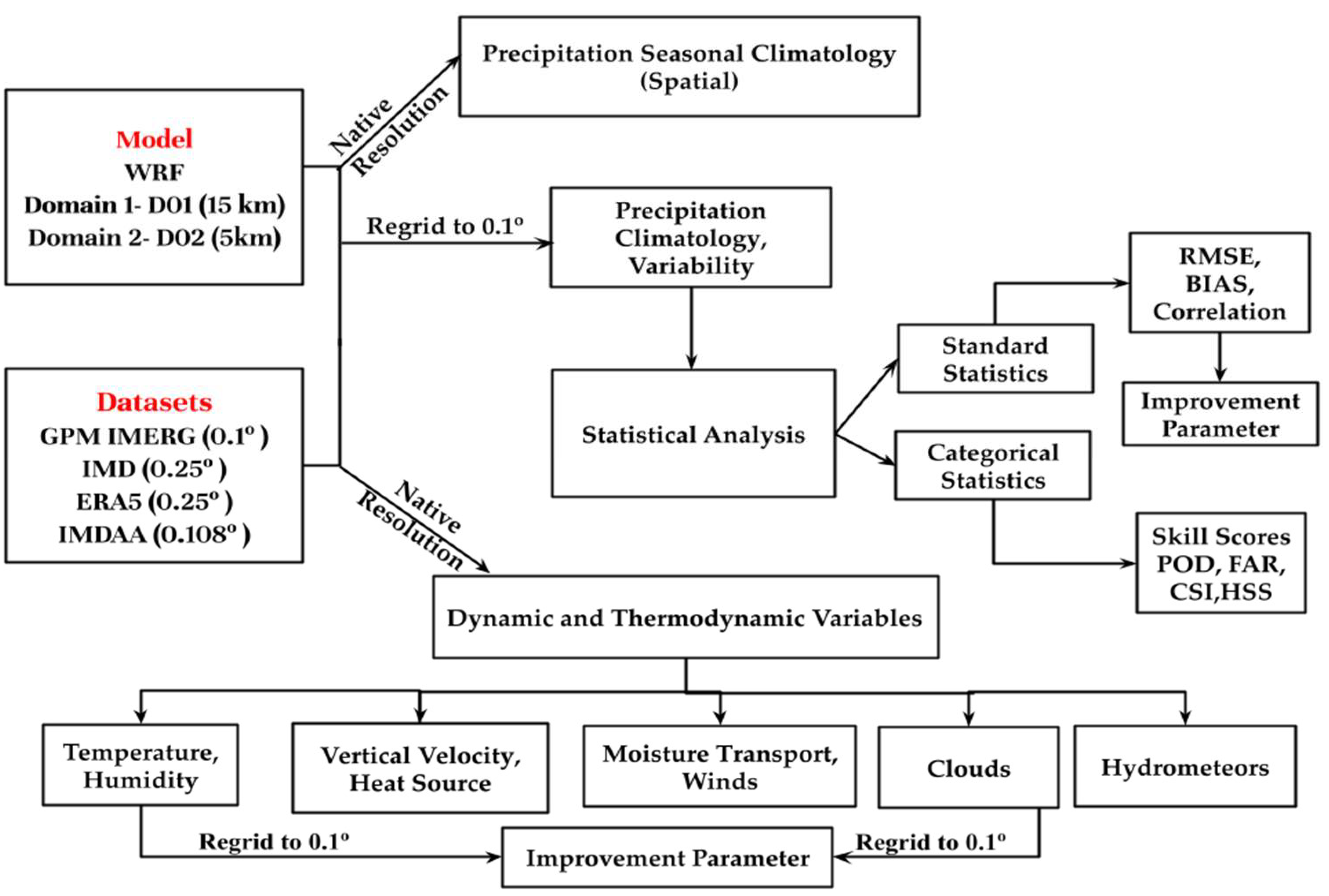
This study evaluates dynamically downscaled WRF winter seasonal precipitation simulations (DJF) over the Western Himalayan region (29° to 37° N; 72° to 82° E) for the period 2001–2016 using different daily precipitation products at their respective spatial resolutions to check the effect of different resolutions in simulating precipitation. Figure 2. shows the flowchart of the methodology used in this study. The seasonal averages were obtained by averaging the daily precipitation measurements for each winter season. Seasonally averaged precipitation, climatology, circulation parameters and hydrometeors were examined to evaluate the model’s ability to capture winter precipitation characteristics. We also compared model-simulated temperature, humidity, geopotential height, vertical velocity, apparent heat source, wind, and cloud cover with IMDAA and ERA5 reanalysis.
To quantitatively assess the model simulations, statistical scores such as mean bias, root-mean-square error (RMSE), BIAS, and the Pearson correlation coefficient (PCC) were computed by re-gridding all the data to a common spatial resolution of 0.1° using bilinear interpolation. The RMSE and BIAS were calculated using seasonally average winter precipitation over each grid point. The computed statistics are briefly mentioned below (see [68] for detailed explanation).
RMSE = i = 1 n ( x i o i ) 2 n                            
BIAS = 1 n i = 1 n ( x i o i )
where x i and o i are the model and observed precipitation for the ith point, and n is the total number of points.
P C C = c o v ( x i , o i ) σ x i   σ o i  
c o v   ( x i ,   o i ) is the covariance between x i and o i (model and observed precipitation, respectively). Here, σ x i and σ o i are the standard deviation of precipitation for the model and the observation, respectively.
Categorical Statistics: We performed a statistical analysis using multiple categorical statistics employing the WRF model results from D01 and D02 as a forecast dataset and IMERG, IMD, ERA5, and IMDAA as the observation/reference datasets [69,70]; https://www.cawcr.gov.au/projects/verification/ accessed on 1 February 2022). All datasets and model results were regrided to 0.1° resolution using bilinear interpolation. The precipitation events in each dataset were divided into four categories using common percentile thresholds across datasets: light (less than the 25th percentile), moderate (between the 25th and 90th percentile), heavy (between the 90th and 95th percentile), and extreme (greater than the 95th percentile) [71]. For each category of events, contingency tables were created, and the associated categorical statistics were generated. The various categorical statistics employed in the study are briefly outlined below.
Probability of Detection (POD): The POD is calculated by dividing the total number of event observations by the number of hits. It has a scale of 0 to 1, with 1 representing the highest score. Thus, it provides a straightforward measurement of the percentage of precipitation events that were accurately predicted or, in this example, recorded by the model.
POD = H M + H
False Alarm Ratio (FAR): The FAR is derived by dividing the number of false alarms by the total number of times an event was forecast. It has a scale of 0 to 1, with 0 representing the highest score. It offers a simple proportionate measurement of the model’s probability of identifying an event when none was actually seen.
FAR = F F + H
Critical Success Index (CSI): The ratio of hits to all events either observed or captured by the model is the CSI, commonly referred to as the threat score. It has a scale of 0 to 1, with 1 representing the highest score.
CSI = H M + H + F
Heidke Skill Score: Heidke skill score is a gauge of forecasting ability. The range of the HSS is −∞ to 1. A flawless forecast results in an HSS of 1, whereas a negative number indicates that the chance forecast is superior, and a 0 indicates no talent.
HSS = ( H + C N )   ( E x p e c t e d C o r r e c t ) N ( E x p e c t e d C o r r e c t )
Expected   Correct   =   1 N { ( H   +   M ) ( H   +   F )   +   ( CN   +   M ) ( CN   +   F ) }
where H = hits—events predicted to occur that did occur; M = misses—events predicted not to occur that did occur; F = false alarms—events predicted to occur that did not occur; CN = correct negative—events predicted not to occur that did not occur; and N = total number of events.
Apart from the evaluation of various model-simulated parameters, we also computed and evaluated vertically integrated moisture transport and apparent heat source for the two model domains using IMDAA and ERA5.
Vertically integrated moisture transport: The vertically integrated moisture transport, VIMT (kg m−1 s −1), was computed as follows:
V I M T = ( 1 g p 0 p T q u d p ) 2 + ( 1 g p 0 p T q v d p ) 2
Here, u is the U-component of wind, v is the V-component of wind, q is the specific humidity, p 0 is pressure at surface, p T is the pressure at the top of the air column, dp is the change in pressure between two levels, and g is the gravity.
Apparent Heat Source: The apparent heat source (Q1, diabatic heating) is computed as the sum of the latent heating associated with phase changes, the vertical transport, the sub-grid diffusion, and the radiative heating (e.g., [72]):
Q 1 = C p ( p p 0 ) k ( θ t + V . θ + ω θ p )
Here, θ is potential temperature, V is horizontal velocity, ω is vertical velocity, p is pressure at a particular pressure level, po is pressure at the surface (1000 mb), k = R/Cp, where R is the gas constant for dry air, and Cp is specific heat at constant pressure.
Forecast impact (IP) parameter: The forecast impact (IP) parameter, a metric to examine the impact of horizontal resolution, quantifies the improvement or degradation in D02 relative to D01 [73]. The method of dividing the D02 error by the D01 error, then multiplying by 100, normalizes the data and provides a measure of the percentage improvement in the predicted parameter with regard to the D01 forecast, which is unrelated to the parameter’s initial value.
IP = [ 1 R M S E D 02 R M S E D 01 ] × 100
where RMSED02 is the root-mean-square error in the D02 predicted variable with respect to a given reference dataset and RMSED01 is the root-mean-square error in D01 with respect to the same reference dataset.

4. Results

4.1. Winter Precipitation Climatology, Variability and Trends over WH

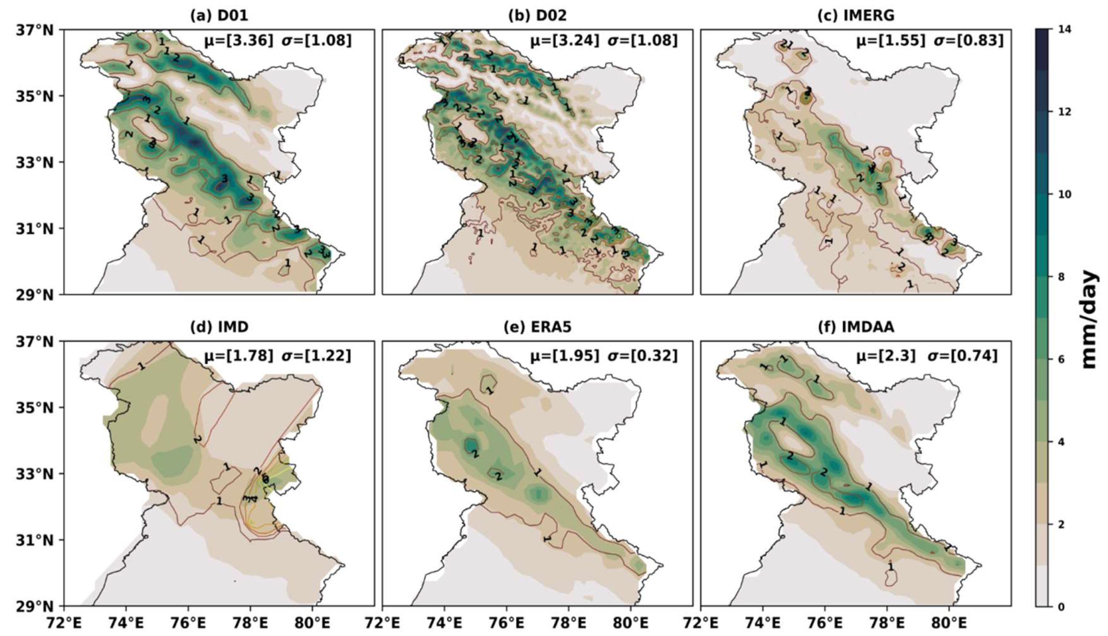
DJF seasonal mean precipitation (shaded) and standard deviation (contours) from the model (D01 and D02) and the available datasets of IMERG, IMD, ERA5, IMDAA, keeping the original resolution of each dataset, are shown in Figure 3. A northwest–southeast-oriented precipitation band extending from the foothills of the Himalayas can be observed in all datasets, indicating that orography plays an important role in the precipitation received in this region. The obtained results are in agreement with previous studies, e.g., [74], and verifies that both domain resolutions are able to capture the precipitation band over WH. However, higher-resolution model simulation (D02) has more detailed precipitation patterns among all datasets, followed by D01. D01 shows relatively homogeneous precipitation patterns compared to D02, thus highlighting the benefits of higher resolution (D02) in capturing localized precipitation patterns. In the northwest–southeast-oriented precipitation band, D01 and D02 show maximum precipitation reaching up to 14 mm/day, IMERG around 13 mm/day, IMD about 4 mm/day, 8 mm/day in ERA5 and, IMDAA shows close to 10 mm/day. Such differences in the obtained precipitation magnitudes for different categories of dataset highlight the challenges that still remain for capturing the spatio-temporal variability of precipitation over WH, thus emphasizing the necessity of high-resolution model simulations. Model-simulated precipitation (D01; D02) is well matched with higher-resolution reanalysis IMDAA compared to other datasets depicting slightly smaller magnitudes. Although the IMERG dataset also has similar resolution, precipitation is confined to the northern side of the precipitation band, and is slightly underestimated compared to WRF-simulated precipitation, similar to what was observed in [21]. D01 shows a highest mean precipitation of 3.36 mm/day, followed by D02 (3.24 mm/day), IMDAA (2.4 mm/day), ERA5 (1.95 mm/day), IMD (1.78 mm/day) and IMERG (1.55 mm/day).
Along the northwest–southeast precipitation band, the spatial variability in precipitation amounts among various datasets can be observed in the reanalysis datasets. IMDAA and ERA5 depict similar precipitation patterns spatially, although differences in precipitation magnitudes are evident, which are attributable to spatial resolution effects, parameterization schemes, and the assimilation techniques used. The lower precipitation magnitudes observed for the high-resolution dataset IMERG corroborates earlier studies, which reported that satellite-based datasets show poorly measured precipitation over high orographic regions [75]. Among all of the datasets, the precipitation band is slightly different in IMD, which could be a result of lacking observed precipitation data, especially over the inaccessible higher reaches of the WH [6,76]. High spatial precipitation variability in the different parts of the region can be observed from the magnitudes of standard deviation (STD). The lowest area averaged STD can be observed in ERA5 followed by IMDAA, IMERG, D01 and D02. Although D01 and D02 show similar area averaged STD, the spatial patterns are much more resolved in the case of D02. In terms of spatial patterns of variability, the depiction of regional precipitation variability seems to be a measure of dataset resolution. D02, with the highest resolution, is able to capture the localized patterns of variability when compared to satellite observations from IMERG and IMDAA reanalysis. D01 also captures the variability, but the finer localized details are missing compared to D02, which is attributable to the effect of resolution, which becomes a very crucial factor in such complex orographic regimes. IMD and ERA5 show very homogeneous patterns for variability, mainly due to their coarser resolution, which might not be sufficient to capture regional precipitation variability for such terrains.
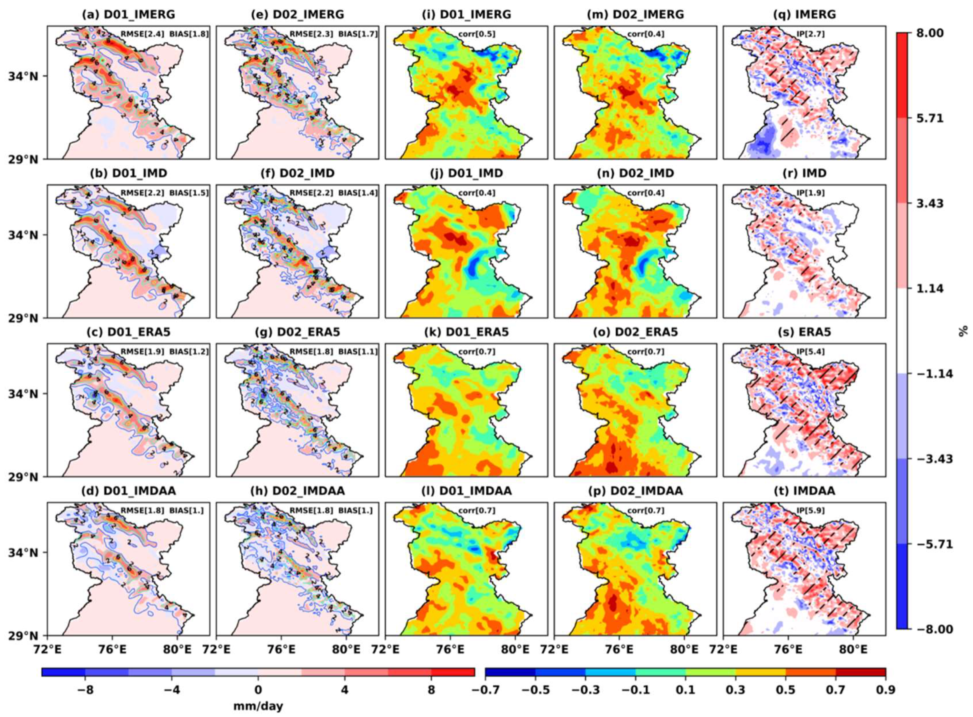
A statistical evaluation of model-simulated precipitation was performed by re-gridding all of the datasets to a common spatial resolution of 0.1 using bilinear interpolation. Figure 4a–h show BIAS (shaded) and RMSE (contours) of precipitation in D01 and D02 with respect to IMERG, IMD, ERA5, IMDAA, respectively. A positive BIAS over the majority of the locations in WH, particularly the major precipitation belt, can be observed in both D01 and D02 with respect to all considered reference datasets. However, the patterns are much more detailed, with sharper boundaries and features in D02 owing to its finer resolution. The largest magnitudes of BIAS are observed over the Karakoram Himalayas, Great Himalayas, and the Himalayan foothills. A slight negative bias over the eastern Ladakh region is observed only in the case of the IMD dataset, a region that contributes a feeble density of gauge network to the gridded dataset IMD, and may not provide true representation of precipitation amounts [77]. The spatial patterns for RMSE show a more or less similar pattern to that seen for BIAS, indicating that regions of high BIAS are also the regions with high RMSE. BIAS and RMSE are mostly observed over locations with high topographic heterogeneity. Such results strongly highlight the fact that the WH region offers significant complexity in terms of precise representation of precipitation amounts, specifically over regions with high topographic variability, and emphasize the necessity of high-resolution data over the region. The patterns are much clearer and more detailed for the higher-resolution domain D02 than for D01, which is similar to results reported by [77], who found a better depiction of patterns in higher-resolution domains. In terms of area-averaged magnitudes, the highest BIAS and RMSE are observed for the IMERG dataset, and the lowest for IMDAA. Overall, D01 and D02 show the lowest BIAS and RMSE with respect to the IMDAA dataset, since it depicts a very similar precipitation pattern to the WRF outputs.
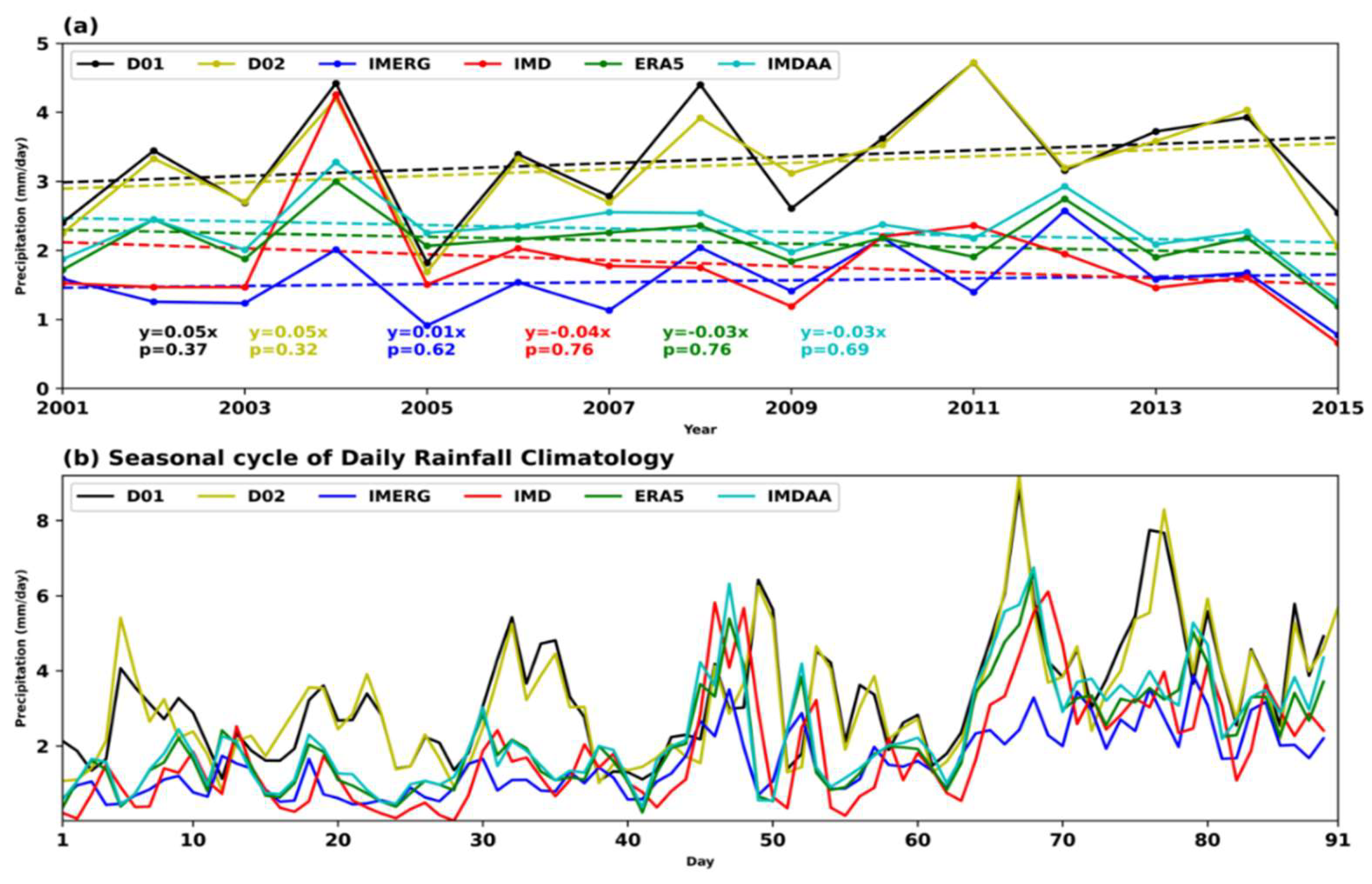
Furthermore, we analyzed the correlation on each grid location for WRF-simulated precipitation in both domains with the individual reference datasets to infer the similarity in terms of grid wise precipitation distribution (Figure 4i–p). The spatial correlations of D01 (D02) with all datasets range between 0.6 and 0.9, with the highest correlation being observed for ERA5 and IMDAA. Figure 4q–t show IP for seasonal precipitation in D02 with respect to D01 for the IMERG, IMD, ERA5, IMDAA datasets, respectively, computed at a confidence level of 95%. D02 depicts some improvement in simulating precipitation compared to D01, thus highlighting the effect of increased spatial resolutions and, in turn, a better resolution of regional orography. The highest percentage of improvement in D02 is observed for IMDAA as the reference dataset, with a mean of 5.9%, followed by ERA5 (5.4%) and IMERG (2.7%), and the lowest is observed for IMD (1.9%). All datasets show a positive IP, specifically across the region with maximum precipitation. Since IP is based on RMSE, lower RMSE values observed earlier with ERA5 and IMDAA datasets cause more improvement with respect to those datasets. Satellite and gauge-based datasets like IMERG and IMD have limitations in terms of obtaining a more detailed picture of precipitation, leading to large RMSE and smaller IP than reanalysis datasets. The area-averaged temporal trends of winter seasonal precipitation from the model simulations and reference datasets over the study region are presented in Figure 5a. Mann–Kendall test [78,79] was used to compute the significance of the observed trends at a confidence level of 95%. Both D01 and D02 show quite similar patterns of interannual variability of precipitation, with well-matched peaks for most years. Increasing trends of winter precipitation are observed for D01, D02, and IMERG, while other datasets show decreasing trends, although all insignificant. The ERA5 and IMDAA precipitation trends are very similar and well matched, although ERA5 presents a slightly lower magnitude than that of IMDAA. We also compared the time series of daily precipitation climatology over the study region (Figure 4b). All datasets are able to capture the variations in the seasonal evolution of precipitation. IMERG exhibits the lowest magnitudes, while D01 and D02 exhibits highest magnitude throughout the time series, and their peaks are well matched. There is an increase in precipitation from the 40th day onwards. More precipitation is received during the months of January and February, which could be due to the fact that more western disturbances are observed during January and February [20].

4.2. Atmospheric Dynamics and Thermodynamics during the Winter Season

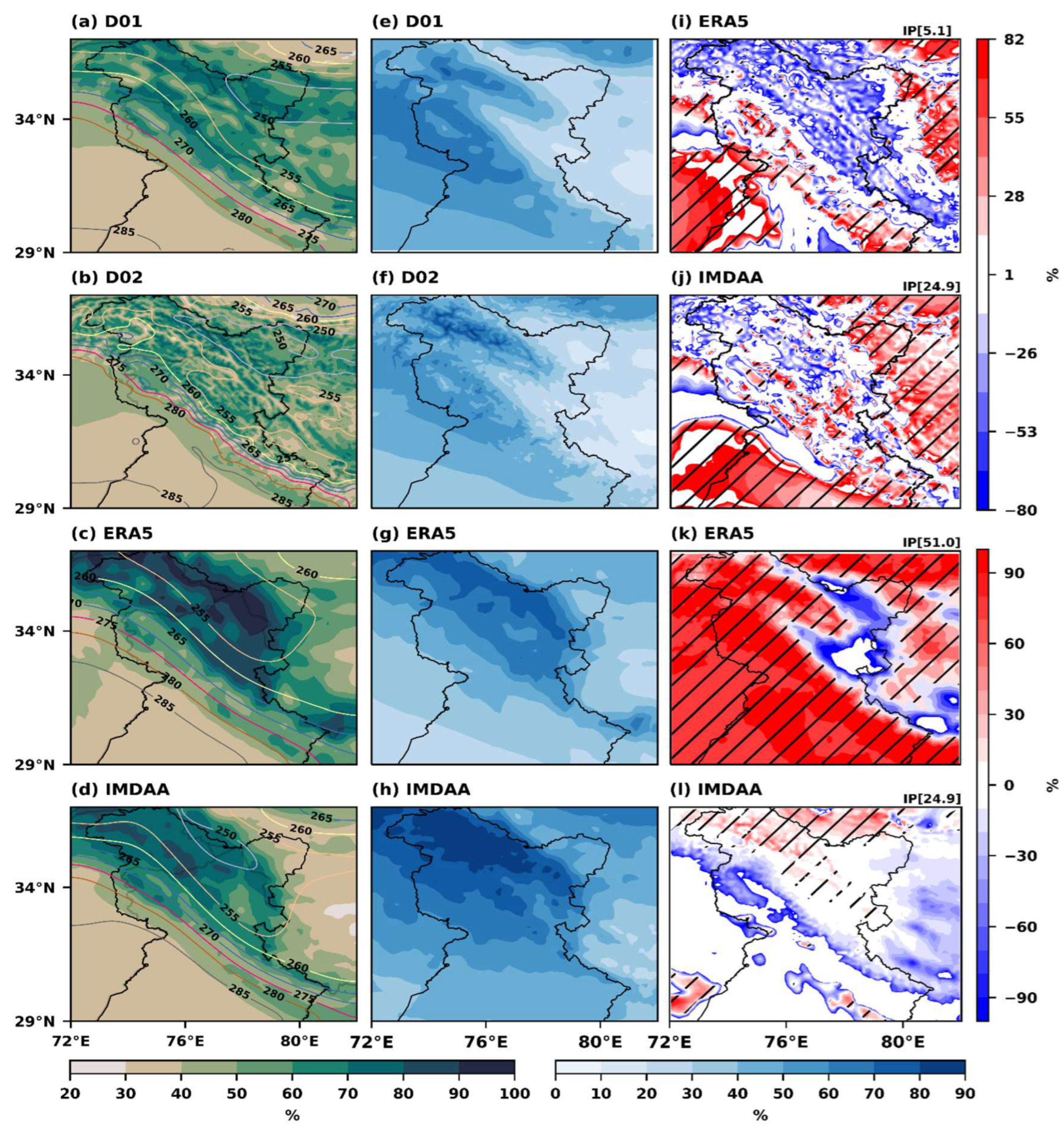
Figure 6a–d present the regional distribution of DJF seasonal climatology of 850 hPa relative humidity (RH; shaded) and 2 m temperature (T2m) in D01, D02, ERA5 and IMDAA, respectively. The results show that the model-simulated temperatures are comparable with the reanalysis datasets. The surface orography pattern is followed by a considerable north–south gradient (>30 K) in T2m between the north Indian plains and the highest elevations of the WH [80]. In winter, T2m cools to about −23 °C or lower at western Himalayan altitudes, while the adjoining north Indian plains remain warm, with mean temperature exceeding 12 °C. The temperature gradient from north to south is better resolved in D02 compared to in D01, ERA5 and IMDAA, which is potentially attributable to the well-represented topography in D02. In high-altitude locations, ERA5 indicates a 5 K warmer T2m than other datasets. RH follows a similar north–south gradient to that observed for T2m. During the winter season, all datasets demonstrate a significant amount of moisture availability over the study region. RH in the lower altitudes ranges between 30% and 40%, whereas it reaches up to 80–90% in the high-altitude regions, thus underlining the role of orography and temperature in deciphering the moisture availability over the region. Among all of the datasets, ERA5 exhibits humidity more than 10 percent higher than in the other datasets. D02 displays the gradient in the RH better than other datasets due to better-resolved orography. In the high-altitude zones, D01 and D02 both slightly underestimate RH compared to ERA5 and IMDAA.
Furthermore, we evaluated total cloud cover in D01 and D02 using ERA5 and IMDAA, respectively (Figure 6e–h). All datasets show similarities in terms of the spatial patterns of cloud cover distribution over the region; however, difference in magnitude are quite evident. Overall, more clouds on the western flank of the study region with a decreasing fraction towards the east can be seen. Similar to the precipitation patterns observed in Figure 3, cloud cover patterns are dense over higher elevations compared to lower orographic regimes. IMDAA and ERA5 both show higher cloud cover over the Karakoram range and the Greater Himalayas, whereas the cloud cover representation in the WRF simulations is highest over the western parts of the Karakoram range and the Greater Himalayas and foothills. Among all datasets, the IMDAA dataset shows the greatest amount of cloud cover (80 to 90 percent) over the northwest part of the study region, whereas other datasets show 50 to 80 percent. We would like to note here that the model cloud cover is well matched with the precipitation patterns observed in the study region, indicating that cloud cover is better represented in the model. Furthermore, we examined whether the enhanced model resolution (D02) offers any improvements in terms of the depiction of RH (Figure 6i–j) and cloud cover (Figure 6k–l) compared to the coarser domain D01. Higher IP in RH can be observed in the model simulations for IMDAA (24.9%) than for ERA5 (5.1%). Moreover, higher IP is seen over the lower altitudes relative to higher orographic regimes, where reduced IP can be observed. This orographic effect is more noticeable in ERA5 than IMDAA. However, IP for cloud cover fractions is significantly larger and more substantial for ERA5 (51%, Figure 6k), and nearly doubles when averaged throughout the region, and, interestingly, is also widely spread compared to IMDAA (24.9%, Figure 6l). However, there are discrepancies between the regional patterns of IP for IMDAA and ERA5.
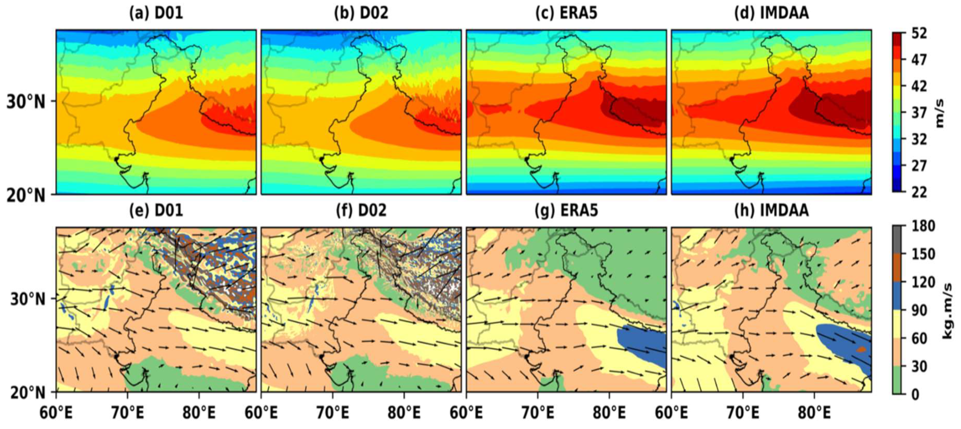
Subtropical westerly jet (200 hPa), the primary carrier of WDs, is the strongest during the winter season, with the axis typically lying over northern India (e.g., [81]). The evaluation of upper tropospheric zonal wind (200 hPa) in D01 and D02 using ERA5 and IMDAA (Figure 7a–d) shows the presence of the jet over the north Indian region. A slight underestimation of the intensity of the model-simulated wind speed can be observed over the region of interest and the surrounding areas, compared to the two reanalysis products. This jet is an important dynamic factor for its contribution to precipitation in the study region. Furthermore, moisture sources in the model are essential for resolving the mechanisms for the development of moist convection and the associated dynamics of precipitation [43]. To investigate the moisture source triggering moist convection and associated rainfall over the WH, the winter means of vertically integrated moisture transport from the surface to 300 hPa from the D01, D02, ERA5 and IMDAA are analyzed and presented in Figure 7e–h, where the vectors represent the direction of moisture transport. The moisture for winter precipitation is generally advected from the westside of the study region through propagation tracks of western disturbances. All datasets—D01, D02, ERA5 and IMDAA—exhibit moisture transport from the west (Figure 7e–h). D01 and D02 show higher values of 120–150 kg m/s for moisture transport over the Himalayan foothills than ERA5 and IMDAA (0–60 kg m/s). This enhanced moisture advection in the model could potentially enhance the precipitation amounts observed in the model simulations compared to those observed in the reanalysis products.
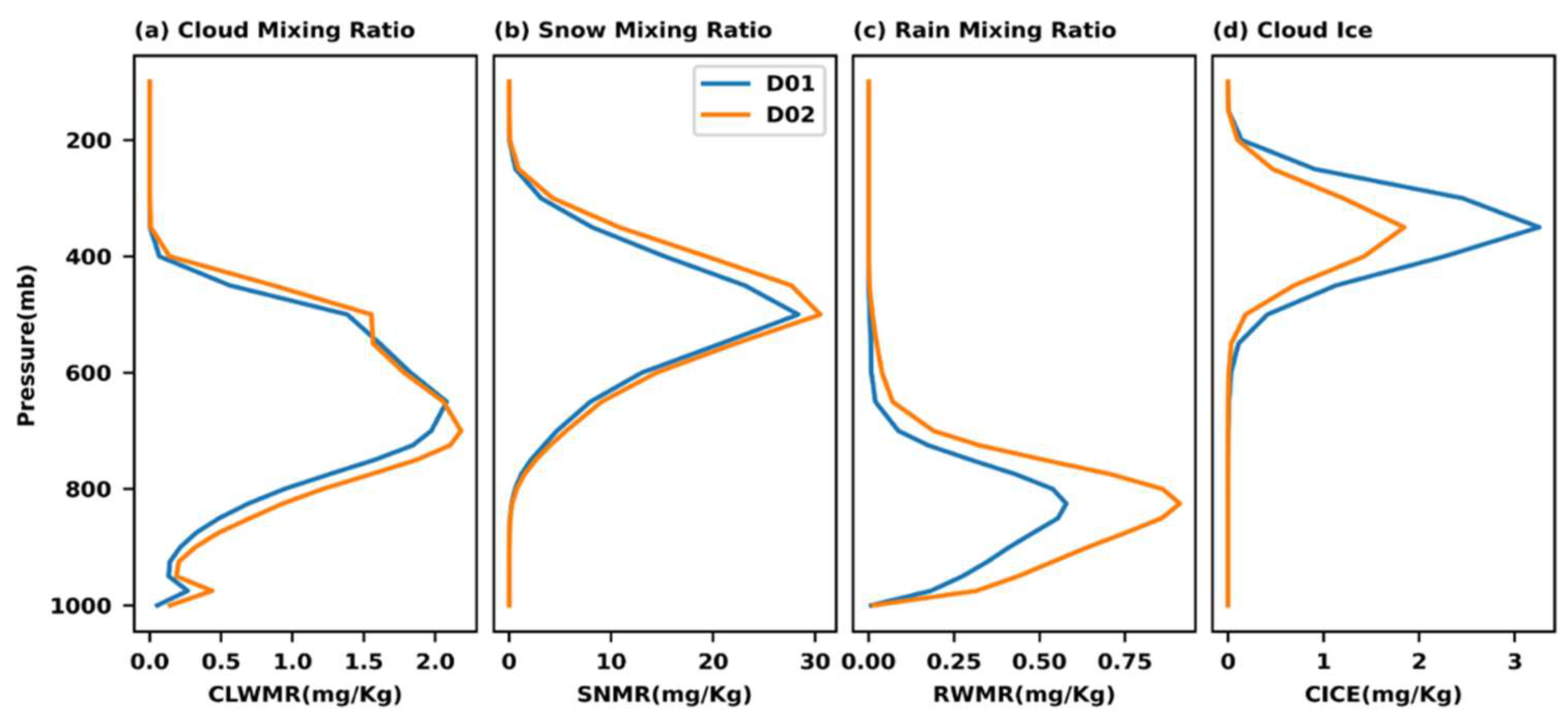
Cloud hydrometeors and their vertical structures have a substantial impact on precipitation processes [43]. Liquid hydrometeors occur below the freezing level, where warm precipitation processes predominate, whereas solid hydrometeors are distributed above the freezing level, where cold precipitation processes predominate. Therefore, a better depiction of cloud hydrometeors is necessary in order to provide realistic model simulations of winter precipitation. The vertical profiles of liquid hydrometeors (cloud and rainwater) and solid hydrometeors (graupel, ice) over the study region are presented in Figure 8. As illustrated in Figure 8a, the results indicate that the cloud water mixing ratio (CLWMR) increases from 1000 mb to 750 mb and then decreases with increasing altitude. CLWMR magnitudes are slightly higher in D02 (peak at 700 mb) than in D01 (peak at 650 mb). The maximum difference in CLWMR is observed between 700 mb and 500 mb (~0.3 mg/kg). The vertical profile of the snow mixing ratio (Figure 8b) indicates that the middle troposphere (500 hPa) is characterized by the maximum snow mixing ratio (SNMR) in both D01 and D02, with D02 presenting a slightly higher SNMR than D01 in the middle to upper troposphere.
As expected, the vertical profile of the rainwater mixing ratio (RWMR; Figure 8c) suggests higher rainwater amounts at lower atmospheric levels (slightly below cloud water) in both D01 and D02, with peaks observed at 825 mb. Raindrops are the only precipitating hydrometeors in the lower troposphere. The resolved RWMR of D02 is comparatively higher that that of D01, with a maximum difference of 0.3 mg/kg at about 825 mb. When compared to the other hydrometeor profiles, the ice mixing ratio (CICE; Figure 8d) reflects availability in the upper troposphere and exhibits its highest peak at 350 hPa for both D01 and D02. CICE values seem to be higher in D01 than in D02, with a maximum observed difference of about ~1.4 mg/kg at 350 mb level, in contrast to all other hydrometeors. RWMR (Figure 8c) is confined to only lower heights, with no large values over 700 hPa being observed. More importantly, this variable has the lowest magnitude (with a maximum of up to 0.5–0.8 mg/kg) among the four hydrometeors evaluated in the present study, while SNMR has the greatest magnitude (with maximum up to 30 mg/kg). CLWMR and SNMR are widespread in the troposphere, while RWMR and CICE are confined to the lower and upper parts of the troposphere, respectively. These findings are consistent with previous research, e.g., [80]. Overall, D02 has higher magnitudes for most hydrometeors, yet identical patterns in vertical distribution profiles for both D02 and D01 can be observed. A clear depiction of hydrometeors aids in the accurate representation of precipitation in model simulations, as seen in D02.
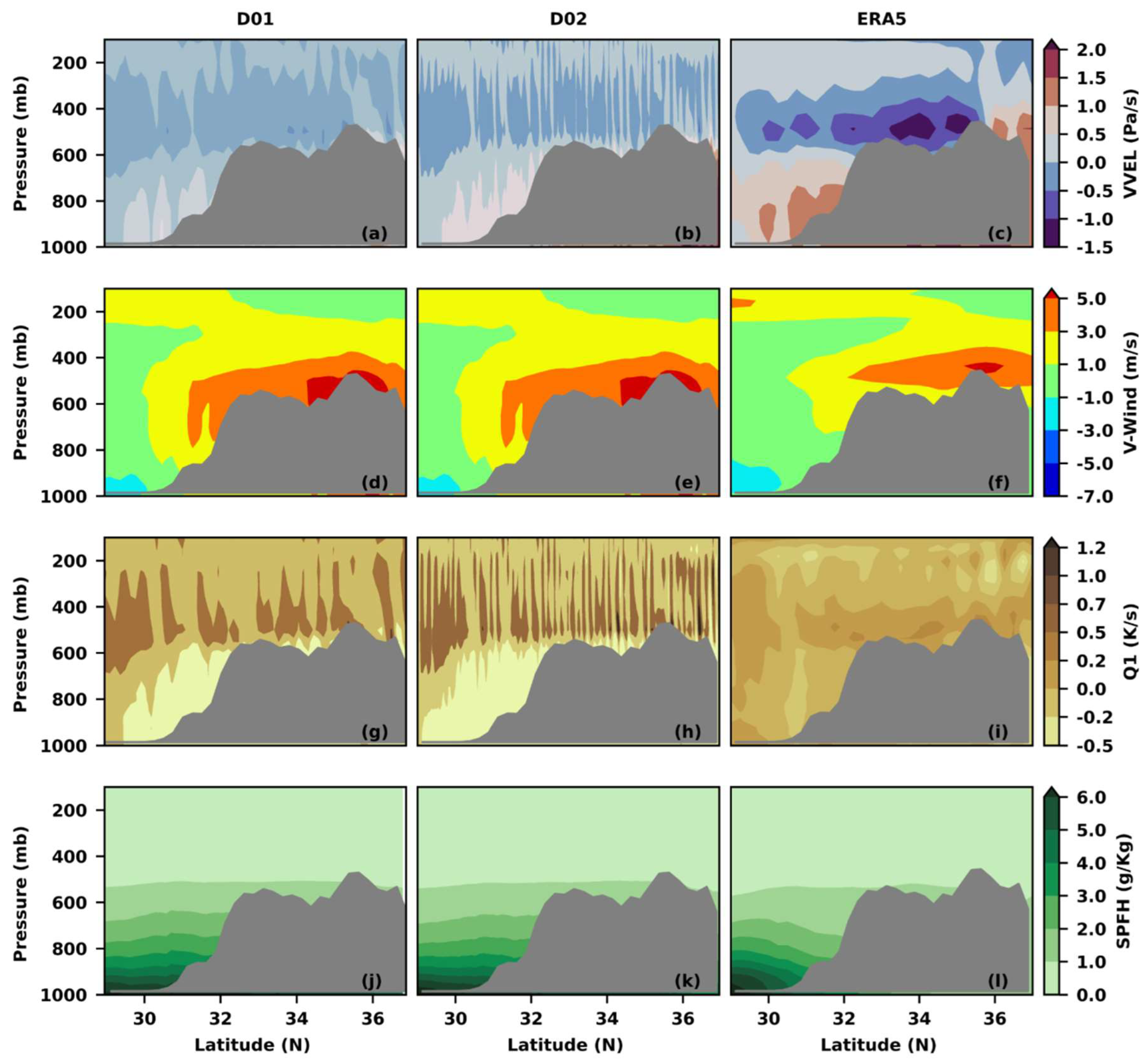
Furthermore, we evaluated the latitude height cross-section of various parameters in D01, D02 with respect to ERA5. In the ERA5 reanalysis, the vertical velocity analysis indicates ascending motion in the atmosphere over the study region. Model simulations are able to reflect these rising motions, although the magnitudes are underestimated. The patterns observed for D02 are substantially sharper and more finely resolved than those for D01 and ERA5, highlighting the advantages offered by higher-resolution data. The plots for meridional winds are presented in Figure 9d–f. The results reveal similarities in vertically distributed patterns of meridional wind in model simulations and ERA5 reanalyses, although slight variations at certain latitudes can be seen. The maximum present at 600 hPa, at latitudes between 34 and 36° N, in ERA5 is well represented in both D01 and D02. The patterns indicate the dominance of southerly winds over the study region. Moreover, the latitudinal extent of southerly wind maxima is higher for D01 and D02 compared to ERA5. The analysis also suggests that topography plays an important role in determining wind patterns over the region, with a lower level at lower latitudes depicting dominance by northerly winds, and southerly winds can be seen over lower latitudes (higher altitudes), higher latitudes (also the region with the maximum elevation in WH), with a maximum velocity of ~4–6 m/s. This separation of southerly and northerly winds helps in the development of westerly troughs over this region [31].
We also investigated the latitude–height distribution of the apparent heat source (Q1, Figure 9g–i) in the atmosphere, which provides vital information about underlying diabatic heating patterns. The patterns observed in ERA5 reveal higher, albeit homogeneous, magnitudes distributed throughout the middle and upper troposphere, with maxima situated between 400 and 600 hPa, indicating enhanced diabatic heating at higher atmospheric levels during the winter season. Both model-simulated domains are able to capture these patterns, with highly detailed representation compared to ERA5, indicating the role played by data resolution. The finest and sharpest features are observed in the case of D02. In contrast to the sizeable diabetic heating in the upper and middle troposphere, lower pressure levels (1000–600 mb) indicate the dominance of diabatic cooling, which is not as strong in ERA5 as it is in the model simulations. Overall, the results emphasize the role of regional topography in modulating the heating and cooling effects over the study region. Additionally, the benefits offered by higher resolution of data for the realistic representation of such effects at a localized scale can also be clearly concluded.
Furthermore, cross-sections for thermodynamic variable specific humidity reveal the presence of higher humidity in the lower atmospheric levels, further decreasing with altitude (less than 1 g/kg above 600 hPa). The patterns for specific humidity observed in the model simulations are remarkably similar to those of ERA5 reanalysis, demonstrating that the model simulations are efficient.

4.3. Skill Scores for Different Rainfall Amounts

Lastly, we attempted to evaluate precipitation events of different intensity on the basis of model simulations with multi-source precipitation datasets. Table 3 depicts the evaluation of various categorical statistics for different types of precipitation event (low, moderate, heavy, extreme) in D01 (D02) against IMERG, IMD, ERA5 and IMDAA. Both domain resolutions have nearly identical POD values for detecting events of all categories when compared to all four precipitation reference datasets. However, the probabilities are higher for moderate events, followed by heavy precipitation events, whereas comparatively lower probabilities of detection seem to be persistent for low and extreme events. In support of the POD values, low FAR values can be observed for moderate- and heavy-precipitation events in both domains relative to the individual reference datasets, whereas the FAR values are relatively high for events of the other two category, with the exception being IMD-based calculations for low-precipitation events. The statistics observed for missing rate for different categories with respect to all reference datasets reveal identical patterns as observed for FAR, indicating that the model simulations depict a higher missing rate for low- and extreme-precipitation events compared to moderate and heavy events. CSI values confirm the findings acquired thus far and indicate that models are capable of identifying moderate and heavy precipitation occurrences with greater success. The model skill was assessed using multi-source datasets (based on different techniques), and the findings show a remarkably similar pattern for all reference datasets. This demonstrates the reliability of the obtained results and clearly indicates that model simulations show higher skill in representing moderate and heavy events, whereas low and extreme events are not depicted clearly. For moderate-precipitation events, the model has the highest level of skill with the IMD dataset, followed by IMDAA, ERA5 and IMERG, while for extreme precipitation, the model has similar skills with all datasets.

5. Discussion and Summary

In this study, we evaluated winter precipitation (2001–2016) over the western Himalayan region using dynamically downscaled model simulations from a regional climate model, WRF, at grey zone horizontal resolutions—15 km (D01) and 5 km (D02)—with various multi-source precipitation datasets (GPM-IMERG, IMD, IMDAA and ERA5). During the winter season, WH receives a significant amount of precipitation through the interaction of WDs with regional orography. A northwest–southeast-oriented precipitation maxima band is observed in the Himalayan foothills, while other regions receive comparatively less precipitation, which is similar to the results reported by [13,31]. Our results highlight the efficiency of the model simulations at both resolutions (D01 and D02) in terms of reproducing the precipitation characteristics over the WH; however, the higher resolution of D02 offers significant advantages in terms of identifying regional precipitation characteristics in detail. When compared to the IMDAA and ERA5 reanalyses, the model outputs are realistic in terms of capturing the spatial patterns of precipitation and their variability, although overestimation occurred for the precipitation magnitudes, which is similar to the findings of [40] regarding RCM-simulated precipitation over WH. The WH region’s orographically induced precipitation is a potential driving factor impacting regional precipitation distribution. Ref. [82] supports the advantages of higher-resolution RCM simulation over other datasets, suggesting that the improved precipitation patterns in RCM are due to a well-presented topography and the fact that RCM uses a higher resolution than reanalysis and other datasets. Both [80,83] reported on the benefits of high resolution in the WRF model for achieving more accurate precipitation simulation. The statistical evaluation of the model-simulated precipitation with various reference datasets reveals the lowest BIAS and RMSE and the highest correlation with the IMDAA dataset. Model simulations showed a wet BIASover the higher elevation zones, with comparatively lowerBIASover the surrounding plains. This might be a result of poorer representation of observations across the mountainous region in other datasets [18,31]. We also observe an improvement in various parameters for D02 simulations compared to D01, which could be attributed to the higher resolution of D02.
A recent study [84] used station data for precipitation trends over WH and reported an increase in winter precipitation from 1971 to 2013. Similarly, Ref. [31] reported an increasing trend in winter precipitation over WH in RCM-simulated precipitation between the years 2000 and 2008. D01 and D02, like [31,84], describe increasing trends for seasonal winter precipitation, which is in agreement with IMERG but in disagreement with other reference datasets. The climatology of winter precipitation demonstrates that the model simulations are also realistic for representing the seasonal cycle of precipitation, although magnitude overestimation is observed. Similar to our findings, Ref. [21] revealed that January and February contributed more than December to winter precipitation. Various categorical and agreement statistics were used to evaluate model simulations in depicting different categories of precipitation events, which revealed the model’s ability to capture moderate and heavy precipitation events efficiently.
Between the north Indian plains and the higher elevations of the Himalayas, a considerable north–south gradient in T2m and RH persists. In comparison to the reference datasets ERA5 and IMDAA, the model simulations are able to capture the north–south gradient for 2 m temperature and 850 hPa relative humidity following surface orography. However, the gradient and spatial patterns in D02 demonstrate comparatively well-marked features and boundaries compared to D01 due to its higher resolution, which helps to resolve the regional orography much more efficiently when using D02. Ref. [80] documented the north–south gradient in 2 m temperature and 850 hPa relative humidity over WH during winter season. The availability of moisture is important for the precipitation to happen. All datasets show a significant amount of moisture availability at 850 mb over the study region. D02 shows a well-presented north–south gradient compared to all other datasets due to the better-resolved orography. D01 and D02 successfully capture the total cloud cover observed in the study region. Cloud cover is found to be much denser over the western parts of the study region compared to the eastern regimes. The effectiveness of higher-resolution D02 at better simulating relative humidity and cloud cover compared to D01 is further confirmed through the observed positive forecast impact (IP) parameters.
The subtropical westerly jet stream is an important factor contributing to the dynamic precipitation during the winter season in the study region. Numerous publications, including [31,82,85], have also reported that the subtropical westerly jet reaches its maximum across northern India during the winter season. The comparison of model-simulated upper-tropospheric winds to reference datasets ERA5 and IMDAA reveal similar patterns, albeit with a slight underestimation of magnitudes, demonstrating the model’s efficacy in simulating the subtropical westerly jet. Ref. [29] reported the underestimation of zonal winds by RCM over WH, which is in agreement with our findings. The wind speeds observed for D01 and D02 are comparable to those noted by [85]. Both D01 and D02 accurately depict the magnitude and direction of vertically integrated moisture transport, which is in line with previous studies [40,85].The distribution of moisture over WH in both model simulations is much more detailed and higher in terms of magnitude than either IMDAA or ERA5, where a comparatively homogeneous pattern can be seen throughout the study region. The higher precipitation amounts observed in D01 and D02 are supported by enhanced moisture transport across the study region in the model simulations compared to the two reanalysis products.
The vertical profiles for solid (ice, snow) and liquid (cloud water, rain water) hydrometeors reveal the capability of the model simulations to reproduce the cloud water and snow mixing ratios present in a large part of the troposphere, while rain water and cloud ice mixing ratio are confined to the lower and upper part of the troposphere, respectively. Ref. [80] discovered comparable hydrometeors mixing ratio in their winter seasonal WRF simulation over WH. Higher values for D02 compared to D01 can be seen generally, which supports the more detailed characterization of precipitation features possible with D02, indicating the advantages offered by its higher resolution.
Lastly, we examined the latitude–pressure cross-sections for vertical velocity, apparent heat source, meridional winds, and specific humidity, revealing the presence of diabatic heating and rising motion in the middle and upper troposphere in D01 and D02 by means of ERA5 reanalysis. The patterns observed in both model simulations are much more detailed and sharper (specifically D02) than ERA5, indicating the role of higher-resolution datasets over such complex topographic regions. The pattern of vertical velocities in our study are similar to what was reported by [85], with ascending motion being observed in the region. Furthermore, the model shows proficiency in simulating the meridional wind pattern and atmospheric specific humidity patterns observed in the study region.

Author Contributions

Conceptualization, R.A.; methodology, P.P., N. and R.A.; formal analysis P.P.; writing—original draft preparation, P.P.; writing—review and editing, R.A., N., P.P., D.A. and C.R.; funding acquisition, R.A. All authors have read and agreed to the published version of the manuscript.

Funding

This research work was supported by the Science and Engineering Research Board, Department of Science and Technology, Government of India under the “Start-up Research Grant (SRG) scheme” (Grant reference SRG/2020/001857).

Institutional Review Board Statement

Not applicable.

Informed Consent Statement

Not applicable.

Data Availability Statement

All the data used in this study are publicly available and accessible. ECMWF fifth generation (ERA5) data are available at https://www.ecmwf.int/en/forecasts/datasets/reanalysis-datasets/era5 (accessed on 1 February 2022). IMDAA data are available on the RDS NCMRWF portal at https://rds.ncmrwf.gov.in/datasets (accessed on 1 February 2022). The GPM-IMERG data are available at https://gpm.nasa.gov/data/directory (accessed on 1 February 2022). The gauge-based datasets can be accessed from https://cdsp.imdpune.gov.in/home_gridded_data.php (accessed on 1 February 2022).

Acknowledgments

The authors gratefully acknowledge NCMRWF, Ministry of Earth Sciences, Government of India, for IMDAA reanalysis. IMDAA reanalysis was produced under the collaboration between UK Met Office, NCMRWF, and IMD with financial support from the Ministry of Earth Sciences, under the National Monsoon Mission programme. Nischal gratefully acknowledges the Prime Minister’s Research Fellowship (PMRF), Ministry of Education, Government of India.

Conflicts of Interest

The authors declare no conflict of interest.

References

  1. Yadav, R.K.; Kumar, K.R.; Rajeevan, M. Characteristic features of winter precipitation and its variability over northwest India. J. Earth Syst. Sci. 2012, 121, 611–623. [Google Scholar] [CrossRef] [Green Version]
  2. Dimri, A.P.; Yasunari, T.; Kotlia, B.S.; Mohanty, U.C.; Sikka, D.R. Indian winter monsoon: Present and past. Earth Sci. Rev. 2016, 163, 297–322. [Google Scholar] [CrossRef]
  3. Hunt, K.M.R.; Curio, J.; Turner, A.G.; Schiemann, R. Subtropical Westerly jet influence on occurrence of Western disturbances and Tibetan Plateau vortices. Geophys. Res. Lett. 2018, 45, 8629–8636. [Google Scholar] [CrossRef] [Green Version]
  4. Tiwari, P.R.; Kar, S.C.; Mohanty, U.C.; Kumari, S.; Sinha, P.; Nair, A.; Dey, S. Skill of precipitation prediction with GCMs over north India during winter season. Int. J. Climatol. 2014, 34, 3440–3455. [Google Scholar] [CrossRef]
  5. Midhuna, T.M.; Kumar, P.; Dimri, A.P. A new Western Disturbance Index for the Indian winter monsoon. J. Earth Syst. Sci. 2020, 129, 59. [Google Scholar] [CrossRef]
  6. Midhuna, T.M.; Dimri, A.P. Future projection of winter precipitation over northwest India and associated regions using CORDEX-SA experiments. Theor. Appl. Climatol. 2020, 139, 1317–1331. [Google Scholar] [CrossRef]
  7. Pisharoty, P.R.; Desai, B.N. Western disturbances and Indian weather. Indian J. Meteor. Geophys. 1956, 8, 333–338. [Google Scholar] [CrossRef]
  8. Mooley, D.A. The role of western disturbances in the production of weather over India during different seasons. Indian J. Meteor. Geophys. 1957, 8, 253–260. [Google Scholar] [CrossRef]
  9. Agnihotri, C.L.; Singh, M.S. Satellite study of western disturbances. Mausam 1982, 33, 249–254. [Google Scholar] [CrossRef]
  10. Dimri, A.P.; Niyogi, D.; Barros, A.P.; Ridley, J.; Mohanty, U.C.; Yasunari, T.; Sikka, D.R. Western Disturbances: A review. Rev. Geophys. 2015, 53, 225–246. [Google Scholar] [CrossRef]
  11. Dimri, A.P.; Niyogi, D. Regional climate model application at subgrid scale on Indian winter monsoon over the western Himalayas. Int. J. Climatol. 2013, 33, 2185–2205. [Google Scholar] [CrossRef]
  12. Ridley, J.; Wiltshire, A.; Mathison, C. More frequent occurrence of westerly disturbances in Karakoram up to 2100. Sci. Total Environ. 2013, 468–469, S31–S35. [Google Scholar] [CrossRef] [PubMed]
  13. Dimri, A.P.; Chevuturi, A.; Niyogi, D.; Thayyen, R.J.; Ray, K.; Tripathi, S.N.; Pandey, A.K.; Mohanty, U.C. Cloudbursts in Indian Himalayas: A review. Earth Sci. Rev. 2017, 168, 1–23. [Google Scholar] [CrossRef]
  14. Chug, D.; Pathak, A.; Indu, J.; Jain, S.K.; Jain, S.K.; Dimri, A.P.; Niyogi, D.; Ghosh, S. Observed evidence for steep rise in the extreme flow of western Himalayan rivers. Geophys. Res. Lett. 2020, 47, e2020GL087815. [Google Scholar] [CrossRef]
  15. Das, J.; Meher, K. Drivers of climate over the Western Himalayan region of India: A review. Earth Sci. Rev. 2019, 198, 102935. [Google Scholar] [CrossRef]
  16. Archer, D.R.; Fowler, H.J. Spatial and temporal variations in precipitation in the Upper Indus Basin, global teleconnections and hydrological implications. Hydrol. Earth Syst. Sci. 2004, 8, 47–61. [Google Scholar] [CrossRef] [Green Version]
  17. Rasmussen, R.; Baker, B.; Kochendorfer, J.; Meyers, T.; Landolt, S.; Fischer, A.P.; Smith, C. How well are we measuring snow: The NOAA/FAA/NCAR winter precipitation test bed. Bull. Am. Meteorol. Soc. 2012, 93, 811–829. [Google Scholar] [CrossRef] [Green Version]
  18. Dimri, A.P.; Yasunari, T.; Wiltshire, A.; Kumar, P.; Mathison, C.; Ridley, J.; Jacob, D. Application of regional climate models to the Indian winter monsoon over the western Himalayas. Sci. Total Environ. 2013, 468–469, S36–S47. [Google Scholar] [CrossRef]
  19. Hussain, S.; Song, X.; Ren, G.; Hussain, I.; Han, D.; Zaman, M.H. Evaluation of gridded precipitation data in the Hindu Kush—Karakoram—Himalaya mountainous area. Hydrol. Sci. J. 2017, 62, 2393–2405. [Google Scholar] [CrossRef]
  20. Baudouin, J.P.; Herzog, M.; Petrie, C.A. Cross-validating precipitation datasets in the Indus River basin. Hydrol. Earth Syst. Sci. 2020, 24, 427–450. [Google Scholar] [CrossRef]
  21. Nischal; Attada, R.; Hunt, K.M. Evaluating winter precipitation over the western Himalayas in a high-resolution Indian regional reanalysis using multi-source climate datasets. J. Appl. Meteorol. Climatol. 2022, 61, 1607–1627. [Google Scholar]
  22. Vergara-Temprado, J.; Ban, N.; Panosetti, D.; Schlemmer, L.; Schär, C. Climate models permit convection at much coarser resolutions than previously considered. J. Clim. 2020, 33, 1915–1933. [Google Scholar] [CrossRef]
  23. White, B.A.; Buchanan, A.M.; Birch, C.E.; Stier, P.; Pearson, K.J. Quantifying the effects of horizontal grid length and parameterized convection on the degree of convective organization using a metric of the potential for convective interaction. J. Atmos. Sci. 2018, 75, 425–450. [Google Scholar] [CrossRef]
  24. Giorgi, F. Thirty years of regional climate modeling: Where are we and where are we going next? J. Geophys. Res. Atmos. 2019, 124, 5696–5723. [Google Scholar] [CrossRef] [Green Version]
  25. Berg, P.; Wagner, S.; Kunstmann, H.; Schädler, G. High resolution regional climate model simulations for Germany: Part I—Validation. Clim. Dyn. 2013, 40, 401–414. [Google Scholar] [CrossRef]
  26. Singh, J.; Singh, N.; Ojha, N.; Sharma, A.; Pozzer, A.; Nadimpally, K.K.; Rajeev, K.; Gunthe, S.S.; Rao, K.V. Effects of spatial resolution on WRF v3.8.1 simulated meteorology over the central Himalaya. Geosci. Model Dev. 2021, 14, 1427–1443. [Google Scholar] [CrossRef]
  27. Rummukainen, M. State-of-the-art with regional climate models. Wiley Interdiscip. Rev. Clim. Change 2010, 1, 82–96. [Google Scholar] [CrossRef]
  28. Srinivas, C.V.; Dasari, H.P.; Rao, D.V.B.; Anjaneyulu, Y.; Baskaran, R.; Venkatraman, B. Simulation of the Indian summer monsoon regional climate using advanced research WRF model. Int. J. Climatol. 2013, 33, 1195–1210. [Google Scholar] [CrossRef]
  29. Attada, R.; Dasari, H.P.; Ghostine, R.; Kondapalli, N.K.; Kunchala, R.K.; Luong, T.M.; Hoteit, I. Diagnostic evaluation of extreme winter rainfall events over the Arabian Peninsula using high-resolution weather research and forecasting simulations. Meteorol. Appl. 2022, 29, e2095. [Google Scholar] [CrossRef]
  30. Jiménez-Esteve, B.; Udina, M.; Soler, M.R.; Pepin, N.; Miró, J.R. Land use and topography influence in a complex terrain area: A high resolution mesoscale modelling study over the Eastern Pyrenees using the WRF model. Atmos. Res. 2018, 202, 49–62. [Google Scholar] [CrossRef] [Green Version]
  31. Kar, S.C.; Tiwari, S.; Tiwari, P.R. High-Resolution Dynamic Downscaling of Winter Climate over the Himalaya. In Climate Change and the White World; Goel, P., Ravindra, R., Chattopadhyay, S., Eds.; Springer: Cham, Switzerland, 2020. [Google Scholar] [CrossRef]
  32. Xue, Y.; Vasic, R.; Janjic, Z.; Mesinger, F.; Mitchell, K.E. Assessment of dynamic downscaling of the continental U.S. regional climate using the Eta/SSiB regional climate model. J. Clim. 2007, 20, 4172–4193. [Google Scholar] [CrossRef]
  33. Lee, D.K.; Cha, D.H.; Kang, H.S. Regional climate simulation of the 1998 summer flood over East Asia. J. Meteorol. Soc. Jpn. 2004, 82, 1735–1753. [Google Scholar] [CrossRef] [Green Version]
  34. Im, E.S.; Park, E.H.; Kwon, W.T.; Giorgi, F. Present climate simulation over Korea with a regional climate model using a one-way double-nested system. Theor. Appl. Climatol. 2006, 86, 187–200. [Google Scholar] [CrossRef]
  35. Gao, X.; Xu, Y.; Zhao, Z.; Pal, J.S.; Giorgi, F. Impacts of horizontal resolution and topography on the numerical simulation of East Asian precipitation. Chin. J. Atmos. Sci. 2006, 30, 185–192. [Google Scholar]
  36. Tang, J.; Zhao, M.; Su, B. Effects of model resolution on the simulation of regionally climatic extreme events. Acta Meteorol. Sin. 2006, 64, 432–442. [Google Scholar]
  37. Dimri, A.P. Impact of horizontal model resolution and orography on the simulation of a western disturbance and its associated precipitation. Meteorol. Appl. 2004, 11, 115–127. [Google Scholar] [CrossRef]
  38. Liu, H.; Zhang, D.L.; Wang, B. Impact of horizontal resolution on the regional climate simulations of the summer 1998 extreme rainfall along the Yangtze River Basin. J. Geophys. Res. Atmos. 2010, 115. [Google Scholar] [CrossRef] [Green Version]
  39. Mishra, A.K.; Kumar, P.; Dubey, A.K.; Javed, A.; Saharwardi, M.S.; Sein, D.V.; Martyanov, S.D.; Jacob, D. Impact of horizontal resolution on monsoon precipitation for CORDEX-South Asia: A regional earth system model assessment. Atmos. Res. 2021, 259, 105681. [Google Scholar] [CrossRef]
  40. Dimri, A.P.; Dash, S.K. Wintertime climatic trends in the western Himalayas. Clim. Change 2012, 111, 775–800. [Google Scholar] [CrossRef]
  41. Vedwan, N.; Rhoades, R.E. Climate change in the Western Himalayas of India: A study of local perception and response. Clim. Res. 2001, 19, 109–117. [Google Scholar] [CrossRef] [Green Version]
  42. Skamarock, W.C.; Klemp, J.B.; Dudhia, J.; Gill, D.O.; Barker, D.; Duda, M.G.; Powers, J.G. A Description of the Advanced Research WRF Version 3; Technical Notes, NCAR/TN-4751STR; NCAR: Boulder, CO, USA, 2018.
  43. Attada, R.; Dasari, H.P.; Kunchala, R.K.; Langodan, S.; Kumar, K.N.; Knio, O.; Hoteit, I. Evaluating cumulus parameterization schemes for the simulation of Arabian Peninsula winter rainfall. J. Hydrometeorol. 2020, 21, 1089–1114. [Google Scholar] [CrossRef] [Green Version]
  44. Raju, A.; Parekh, A.; Kumar, P.; Gnanaseelan, C. Evaluation of the impact of AIRS profiles on prediction of Indian summer monsoon using WRF variational data assimilation system. J. Geophys. Res. Atmos. 2015, 120, 8112–8131. [Google Scholar] [CrossRef]
  45. Mishra, P.; Kannan, S.R.; Radhakrishnan, C. The Effect of Anthropogenic Heat and Moisture on Local Weather at Industrial Heat Islands: A Numerical Experiment. Atmosphere 2022, 13, 357. [Google Scholar] [CrossRef]
  46. Chandrasekar, R.; Balaji, C. Sensitivity of Tropical Cyclone Jal Simulations to Physics Parameterisations. J. Earth Syst. Sci. 2012, 121, 923–946. [Google Scholar] [CrossRef] [Green Version]
  47. Subramani, D.; Chandrasekar, R.; Ramanujam, K.S.; Balaji, C. A New Ensemble-Based Data Assimilation Algorithm to Improve Track Prediction of Tropical Cyclones. Nat. Hazard. 2014, 71, 659–682. [Google Scholar] [CrossRef]
  48. Chandrasekar, R.; Balaji, C. Impact of Physics Parameterisation and 3DVAR Data Assimilation on Prediction of Tropical Cyclones in the Bay of Bengal Region. Nat. Hazard. 2016, 80, 223–247. [Google Scholar] [CrossRef]
  49. Chandrasekar, R.; Sahu, R.K.; Balaji, C. Assimilation of multi-channel radiances in mesoscale models with an ensemble technique to improve track forecasts of Tropical cyclones. J. Earth Syst. Sci. 2022, 131, 83. [Google Scholar] [CrossRef]
  50. Mittal, R.; Tewari, M.; Radhakrishnan, C.; Ray, P.; Singh, T.; Nickerson, A. Response of Tropical Cyclone Phailin (2013) in the Bay of Bengal to Climate Perturbations. Clim. Dyn. 2019, 53, 2013–2030. [Google Scholar] [CrossRef]
  51. Ansari, T.U.; Ojha, N.; Chandrasekar, R.; Balaji, C.; Singh, N.; Gunthe, S.S. Competing Impact of Anthropogenic Emissions and Meteorology on the Distribution of Trace Gases Over Indian Region. J. Atmos. Chem. 2016, 73, 363–380. [Google Scholar] [CrossRef]
  52. Radhakrishnan, C.; Chandrasekar, V. CASA Prediction System over Dallas—Fort Worth Urban Network: Blending of Nowcasting and High-Resolution Numerical Weather Prediction Model. J. Atmospheric Ocean. Technol. 2020, 37, 211–228. [Google Scholar] [CrossRef]
  53. Ramanujam, S.; Chandrasekar, R.; Chakravarthy, B. A New PCA-ANN Algorithm for Retrieval of Rainfall Structure in a Precipitating Atmosphere. Int. J. Numer. Method. Heat Fluid Flow 2011, 21, 1002–1025. [Google Scholar] [CrossRef]
  54. Ramanujam, S.; Radhakrishnan, C.; Subramani, D.; Chakravarthy, B. On the Effect of Non-Raining Parameters in Retrieval of Surface Rain Rate Using TRMM PR and TMI Measurements. IEEE J. Sel. Top. Appl. Earth Obs. Remote Sens. 2012, 5, 735–743. [Google Scholar] [CrossRef]
  55. Balaji, C.; Krishnamoorthy, C.; Chandrasekar, R. On the Possibility of Retrieving Near-Surface Rain Rate from the Microwave Sounder SAPHIR of the Megha-Tropiques Mission. Curr. Sci. 2014, 106, 587–593. [Google Scholar]
  56. Kain, J.S. The Kain—Fritsch convective parameterization: An update. J. Appl. Meteor. 2004, 43, 170–181. [Google Scholar] [CrossRef]
  57. Kain, J.S.; Fritsch, J.M. Convective parameterization for mesoscale models: The Kain—Fritsch scheme. The Representation of Cumulus Convection in Numerical Models. In Meteorological Monographs; American Meteorological Society: Boston, MA, USA, 1993; pp. 165–170. [Google Scholar]
  58. Thompson, G.; Tewari, M.; Ikeda, K.; Tessendorf, S.; Weeks, C.; Otkin, J.A.; Kong, F. Explicitly-coupled cloud physics and radiation parameterizations and subsequent evaluation in WRF high-resolution convective forecasts. Atmos. Res. 2016, 168, 92–104. [Google Scholar] [CrossRef] [Green Version]
  59. Nakanishi, M.; Niino, H. An improved Mellor—Yamada level-3 model with condensation physics: Its design and verification. Bound. Layer Meteorol. 2004, 112, 1–31. [Google Scholar] [CrossRef]
  60. Iacono, M.J.; Delamere, J.S.; Mlawer, E.J.; Shephard, M.W.; Clough, S.A.; Collins, W.D. Radiative forcing by long lived greenhouse gases: Calculations with the AER radiative transfer models. J. Geophys. Res. 2008, 113, D13103. [Google Scholar] [CrossRef]
  61. Chen, F.; Dudhia, J. Coupling an advanced land surface hydrology model with the Penn State—NCAR MM5 modelling system. Part I: Model implementation and sensitivity. Mon. Weather. Rev. 2001, 129, 569–585. [Google Scholar] [CrossRef]
  62. Hersbach, H.; Bell, B.; Berrisford, P.; Hirahara, S.; Horányi, A.; Muñoz-Sabater, J.; Nicolas, J.; Peubey, C.; Radu, R.; Schepers, D.; et al. The ERA5 global reanalysis. Q. J. R. Meteorol. Soc. 2020, 146, 1999–2049. [Google Scholar] [CrossRef]
  63. Ashrit, R.; Rani, S.I.; Kumar, S.; Karunasagar, S.; Arulalan, T.; Francis, T.; Routray, A.; Laskar, S.I.; Mahmood, S.; Jermey, P.; et al. IMDAA regional reanalysis: Performance evaluation during Indian summer monsoon season. J. Geophys. Res. Atmos. 2020, 125, e2019JD030973. [Google Scholar] [CrossRef]
  64. Rani, S.I.; Arulalan, T.; George, J.P.; Rajagopal, E.N.; Renshaw, R.; Maycock, A.; Barker, D.M.; Rajeevan, M. IMDAA: High resolution satellite-era reanalysis for the Indian monsoon region. J. Clim. 2021, 34, 5109–5133. [Google Scholar] [CrossRef]
  65. Pai, D.S.; Latha, S.; Rajeevan, M.; Sreejith, O.P.; Satbhai, N.S.; Mukhopadhyay, B. Development of a new high spatial resolution (0.25° × 0.25°) long period (1901–2010) daily gridded rainfall data set over India and its comparison with existing data sets over the region. Mausam 2014, 65, 1–18. [Google Scholar] [CrossRef]
  66. Huffman, G.J.; Bolvin, D.T.; Braithwaite, D.; Hsu, K.; Joyce, R.; Kidd, C.; Xie, P. NASA Global Precipitation Measurement Integrated MultisatellitE Retrievals for GPM (IMERG). In Algorithm Theoretical Basis Document, Version 4.5; NASA: Washington, DC, USA, 2015. [Google Scholar]
  67. Huffman, G.; Bolvin, D.; Braithwaite, D.; Hsu, K.; Joyce, R. NASA global precipitation measurement (GPM) integrated multi-satellitE Retrievals for GPM (IMERG). In Algorithm Theoretical Basis Document (ATBD); NASA: Washington, DC, USA, 2019. [Google Scholar]
  68. Zandler, H.; Haag, I.; Samimi, C. Evaluation needs and temporal performance differences of gridded precipitation products in peripheral mountain regions. Sci. Rep. 2019, 9, 15118. [Google Scholar] [CrossRef] [PubMed]
  69. Thornes, J.; Stephenson, E.; David, B. How to judge the quality and value of weather forecast products. Meteorol. Appl. 2001, 8, 307–314. [Google Scholar] [CrossRef] [Green Version]
  70. Mcbride, J.L.; Ebert, E.E. Verification of quantitative precipitation forecasts from operational numerical weather prediction models over Australia. Weather Forecast. 2000, 15, 103–121. [Google Scholar] [CrossRef]
  71. Aggarwal, D.; Attada, R.; Shukla, K.K.; Chakraborty, R.R.; Kunchala, K. Monsoon precipitation characteristics and extreme precipitation events over Northwest India using Indian high-resolution regional reanalysis. Atmos. Res. 2022, 267, 105993. [Google Scholar] [CrossRef]
  72. Liu, C.; Moncrieff, M.W. Sensitivity of cloud-resolving simulations of warm season convection to cloud microphysics parameterizations. Mon. Weather Rev. 2007, 135, 2854–2868. [Google Scholar] [CrossRef]
  73. Wilks, D. Statistical Methods in the Atmospheric Sciences: An Introduction, 3rd ed.; Academic Press: London, UK, 2011. [Google Scholar]
  74. Dimri, A.P.; Mohanty, U.C. Simulation of mesoscale features associated with intense western disturbances over western Himalayas. Meteorol. Appl. 2009, 16, 289–308. [Google Scholar] [CrossRef]
  75. Kanda, N.; Negi, H.S.; Rishi, M.S.; Kumar, A. Performance of Various Gridded Temperature and Precipitation Datasets over Northwest Himalayan Region. Environ. Res. Commun. 2020, 2, 85002. [Google Scholar] [CrossRef]
  76. Ménégoz, M.; Gallée, H.; Jacobi, H.W. Precipitation and snow cover in the Himalaya: From reanalysis to regional climate simulations. Hydrol. Earth Syst. Sci. 2013, 17, 3921–3936. [Google Scholar] [CrossRef] [Green Version]
  77. Kishore, P.; Jyothi, S.; Basha, G.; Rao, S.V.B.; Rajeevan, M.; Velicogna, I.; Sutterley, T.C. Precipitation climatology over India: Validation with observations and reanalysis datasets and spatial trends. Clim. Dyn. 2016, 46, 541–556. [Google Scholar] [CrossRef] [Green Version]
  78. Kendall, M.G. Rank Correlation Methods, 4th ed.; Charles Griffin: London, UK, 1975. [Google Scholar]
  79. Mann, H.B. Non-parametric test against trend. Econometrica 1945, 13, 245–259. [Google Scholar] [CrossRef]
  80. Tiwari, S.; Kar, S.C.; Bhatla, R. Dynamic downscaling over western Himalayas: Impact of cloud microphysics schemes. Atmos. Res. 2018, 201, 1–16. [Google Scholar] [CrossRef]
  81. Hunt, K.M.; Turner, A.G.; Shaffrey, L.C. The evolution, seasonality and impacts of western disturbances. Q. J. R. Meteorol. Soc. 2018, 144, 278–290. [Google Scholar] [CrossRef] [Green Version]
  82. Hunt, K.M.R.; Turner, A.G.; Shaffrey, L.C. The impacts of climate change on the winter water cycle of the western Himalaya. Clim. Dyn. 2020, 55, 2287–2307. [Google Scholar] [CrossRef]
  83. Norris, J.; Carvalho, L.M.V.; Jones, C.; Cannon, F.; Bookhagen, F.; Palazzi, E.; Tahir, A.A. The spatiotemporal variability of precipitation over the Himalaya: Evaluation of one-year WRF model simulation. Clim. Dyn. 2017, 49, 2179–2204. [Google Scholar] [CrossRef]
  84. Shekhar, M.S.; Rao, N.N.; Paul, S.; Bhan, S.C.; Singh, G.P.; Singh, A. Winter precipitation climatology over Western Himalaya: Altitude and Range wise study. J. Indian Geophys. Union 2017, 21, 148–152. [Google Scholar]
  85. Nageswararao, M.M.; Mohanty, U.C.; Osuri, K.K.; Ramakrishna, S.S.V.S. Prediction of winter precipitation over northwest India using ocean heat fluxes. Clim. Dyn. 2016, 47, 2253–2271. [Google Scholar] [CrossRef]
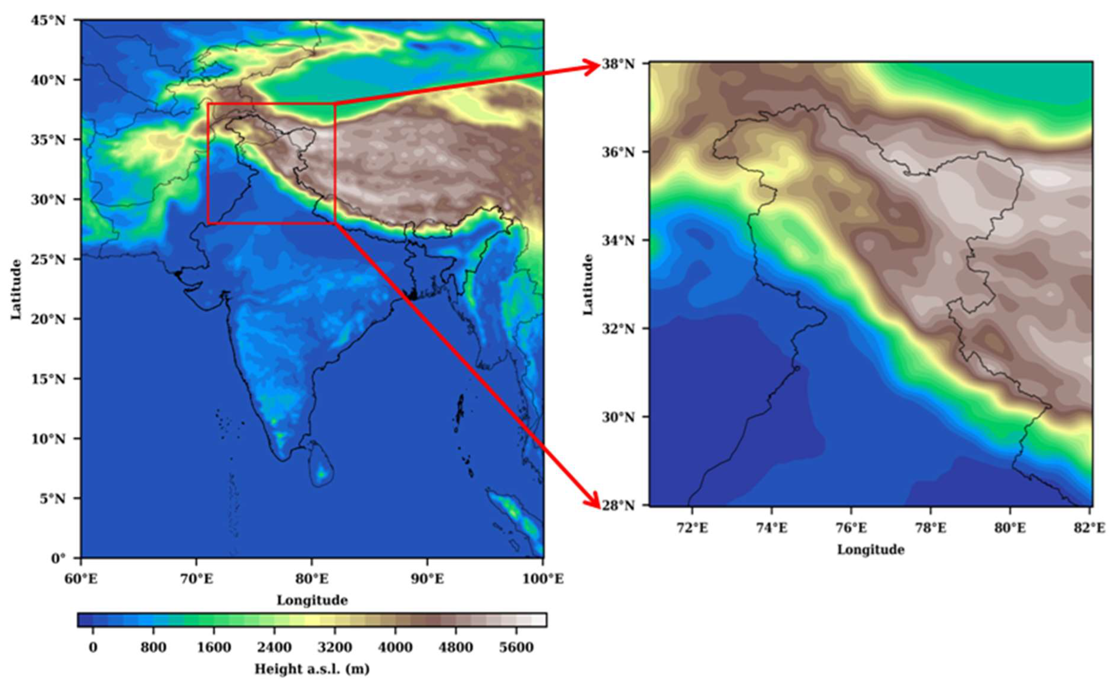
Figure 1. Topographic map from WRF, where the outlined box is the study region.
Climate 10 00160 g001
Figure 2. Flowchart of the methodology used in this study.
Climate 10 00160 g002
Figure 3. Seasonal (DJF) average precipitation captured by WRF model; D01 (a), D02 (b) and precipitation products; IMERG (c), IMD (d), ERA5 (e) and IMDAA (f). Shading and contours represent the magnitude of seasonal average precipitation and standard deviation, respectively.
Climate 10 00160 g003
Figure 4. Seasonal precipitation difference (BIAS) between model and observations: (a) D01-IMERG, (b) D01-IMD, (c) D01-ERA5, (d) D01-IMDAA, (e) D02-IMERG, (f) D02-IMD, (g) D02-ERA5, and (h) D02-IMDAA, shading and contours represent the BIAS and RMSE, respectively. Seasonal precipitation correlation between model and observations: (i) D01-IMERG, (j) D01-IMD, (k) D01-ERA5, (l) D01-IMDAA, (m) D02-IMERG, (n) D02-IMD, (o) D02-ERA5, and (p) D02-IMDAA, shading and contours represent the BIAS and RMSE, respectively. Forecast impact parameter for model-simulated seasonal precipitation against (q) IMERG, (r) IMD, (s) ERA5 and (t) IMDAA for the period 2001–2016.
Climate 10 00160 g004
Figure 5. Temporal trends in area-averaged seasonal (DJF) precipitation (a) and daily climatology of area averaged precipitation (b).
Climate 10 00160 g005
Figure 6. Seasonal average RH and Temperature at 2 m above the ground, observed in model (a) D01 and (b) D02 and observations (c) ERA5 and (d) IMDAA. Shading and contours represent the RH and temperature, respectively. Seasonal averaged total cloud cover between the models and (e) D01 and (f) D02 and the observations (g) ERA5 and (h) IMDAA. The seasonal forecast impact (IP) parameter for RH and total cloud cover with ERA5 (i), IMDAA (j), ERA5 (k), and IMDAA (l), respectively.
Climate 10 00160 g006
Figure 7. Seasonal averaged zonal winds at 200 mb in model D01 (a) and D02 (b) and observation ERA5 (c) and IMDAA (d). Seasonal averaged vertically integrated moisture transport between 1000 and 300 mb in model D01 (e) and D02 (f) and observations ERA5 (g) and IMDAA (h).
Climate 10 00160 g007
Figure 8. Area-averaged seasonal cloud hydrometeor mixing ratio observed in model simulations.
Climate 10 00160 g008
Figure 9. Latitudinal cross-section of vertical velocity observed in D01 (a), D02 (b), ERA5 (c); meridional component of wind observed in D01 (d), D02 (e), ERA5 (f); apparent heat source observed in D01 (g), D02 (h), ERA5 (i); specific humidity observed in D01 (j), D02 (k), ERA5 (l) along longitude 76.88° E.
Climate 10 00160 g009
Table 1. Details for WRF model configurations and physical parameterization schemes used in this study.
WRF Model Setup
Initial, lateral boundary conditionEuropean Centre for Medium-Range Weather Forecasts Interim Reanalysis (ERAI) (0.758°)
Domain extends30 °W–130 °E, 30 °S–45 °N
Convective Parameterization SchemeKF scheme [42,51]
Microphysical schemeThompson scheme [53]
Radiation schemes
(Shortwave, Longwave)
Rapid Radiative Transfer Model for global circulation models (RRTMG) [55]
Planetary boundary layer schemeMellor–Yamada–Nakanishi–Niino turbulent kinetic energy scheme [54]
Land surface schemeNoah land surface model scheme [56]
Table 2. Various datasets used in this study, along with their spatial and temporal resolutions.
Dataset Spatial
Coverage
Temporal
Coverage
Spatial ResolutionTemporal
Resolution
Reference
GPM-IMERGGlobal2001–20160.1° × 0.1°Half hourlyHuffman et al., 2015 [61]
IMD India 2001–20160.25° × 0.25°DailyPai et al., 2014 [60]
ERA5 Global2001–2016 0.25° × 0.25°1 hourlyHersbach et al., 2020 [57]
IMDAA South Asia and
adjoining regions
2001–20160.108° × 0.108°1 hourly, 3-hourlyRani et al., 2021 [59]
Table 3. Categorical statistics for the examination of the model’s ability to detect (area averaged) low, moderate, heavy, and extreme precipitation events during DJF months against that of IMERG, IMD, ERA5 and IMDAA.
IMERGIMD
D01 (D02)<25 P25–90 P90–95 P>95 P<25 P25–90 P90–95 P>95 P
POD 0.42 (0.38)0.65 (0.65)0.52 (0.52)0.31 (0.28)0.04 (0.02)0.86 (0.86)0.52 (0.52)0.41 (0.36)
FAR 0.65 (0.70)0.26 (0.26)0.49 (0.49)0.91 (0.91)0.00 (0.00)0.01 (0.01)0.49 (0.49)0.78 (0.81)
CSI 0.24 (0.20)0.53 (0.53)0.35 (0.35)0.08 (0.07)0.04 (0.02)0.79 (0.79)0.35 (0.35)0.17 (0.14)
HSS 0.15 (0.07)0.01 (0.01)0.00 (0.00)0.08 (0.06)0.06 (0.03)0.15 (0.16)0.00 (0.00)0.24 (0.20)
ERA5IMDAA
D01 (D02)<25 P25–90 P90–95 P>95 P<25 P25–90 P90–95 P>95 P
POD0.36 (0.40)0.73 (0.72)0.52 (0.52)0.28 (0.27)0.36 (0.38)0.74 (0.73)0.52 (0.52)0.34 (0.30)
FAR 0.55 (0.56)0.26 (0.26)0.49 (0.49)0.84 (0.85)0.54 (0.57)0.26 (0.26)0.49 (0.49)0.79 (0.82)
CSI 0.25 (0.26)0.53 (0.53)0.35 (0.35)0.11 (0.11)0.26 (0.26)0.59 (0.59)0.35 (0.35)0.15 (0.13)
HSS 0.23 (0.23)0.03 (0.03)0.00 (0.00)0.15 (0.13)0.24 (0.23)0.03 (0.03)0.00 (0.00)0.21 (0.18)
Publisher’s Note: MDPI stays neutral with regard to jurisdictional claims in published maps and institutional affiliations.