
Wave Analysis for Offshore Aquaculture Projects: A Case Study for the Eastern Mediterranean Sea


Abstract
:1. Introduction
1.1. Aquaculture: Shifting from Coastal to Offshore
1.2. Literature Review
1.3. Aim of Work
2. Data
2.1. Description
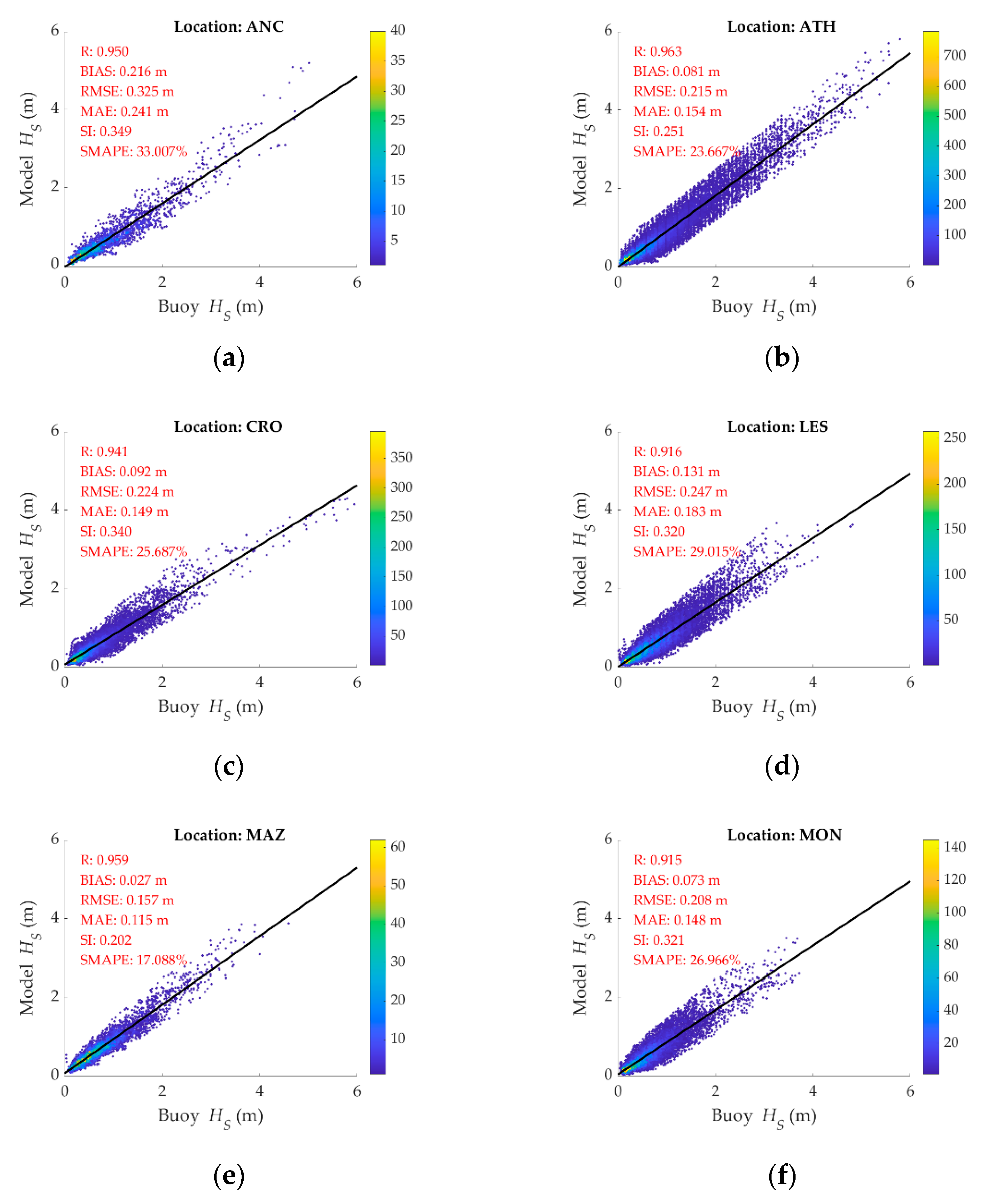
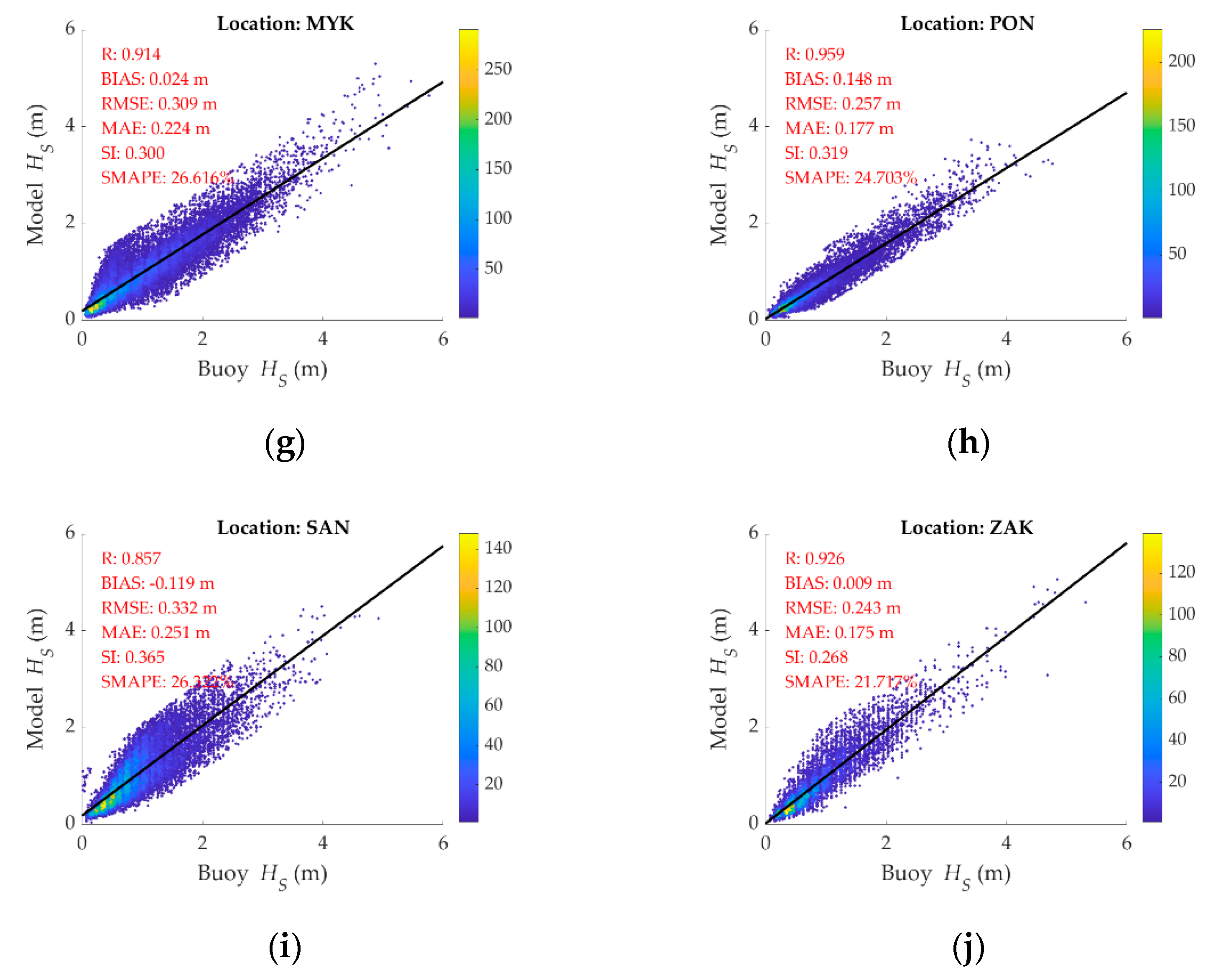
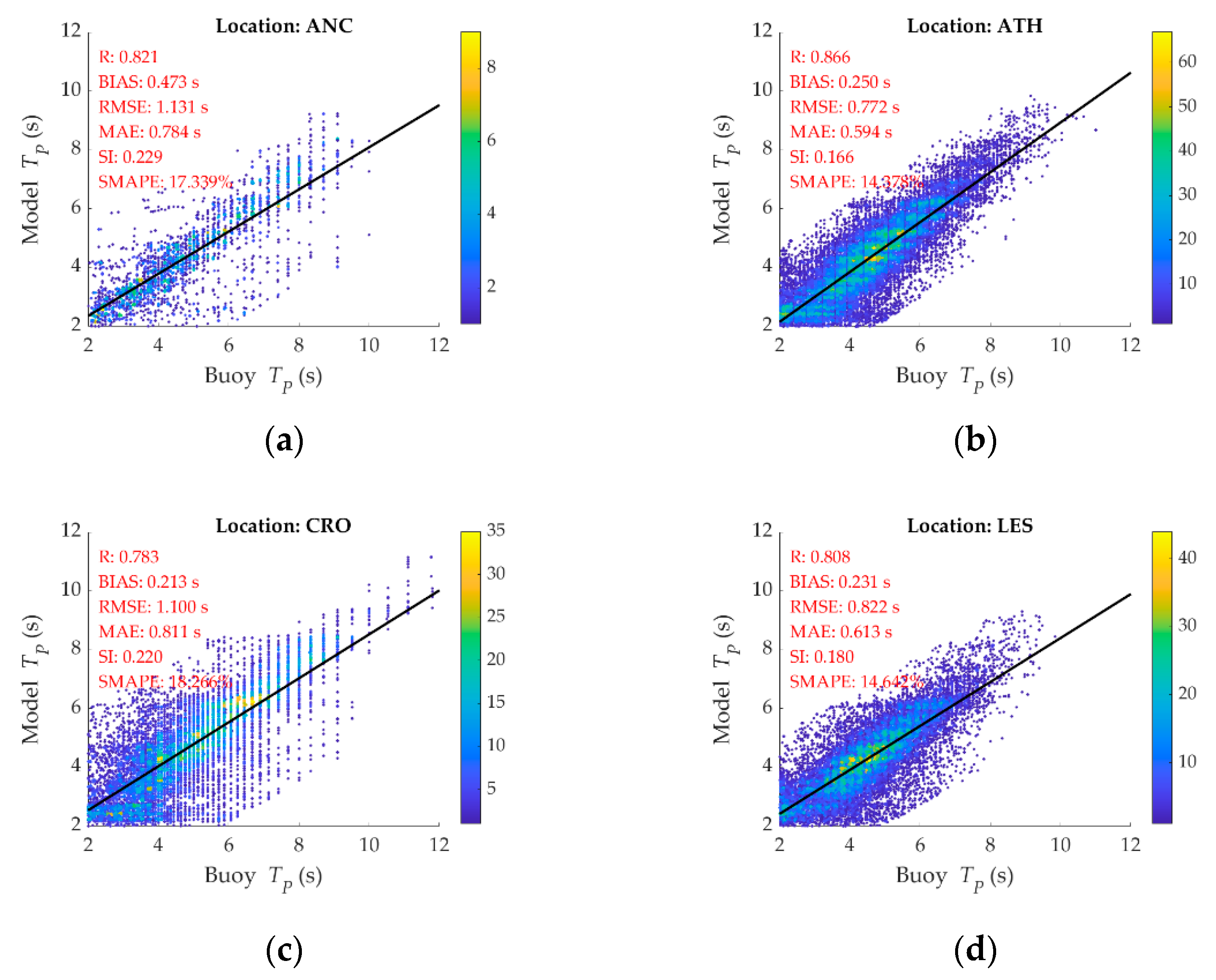
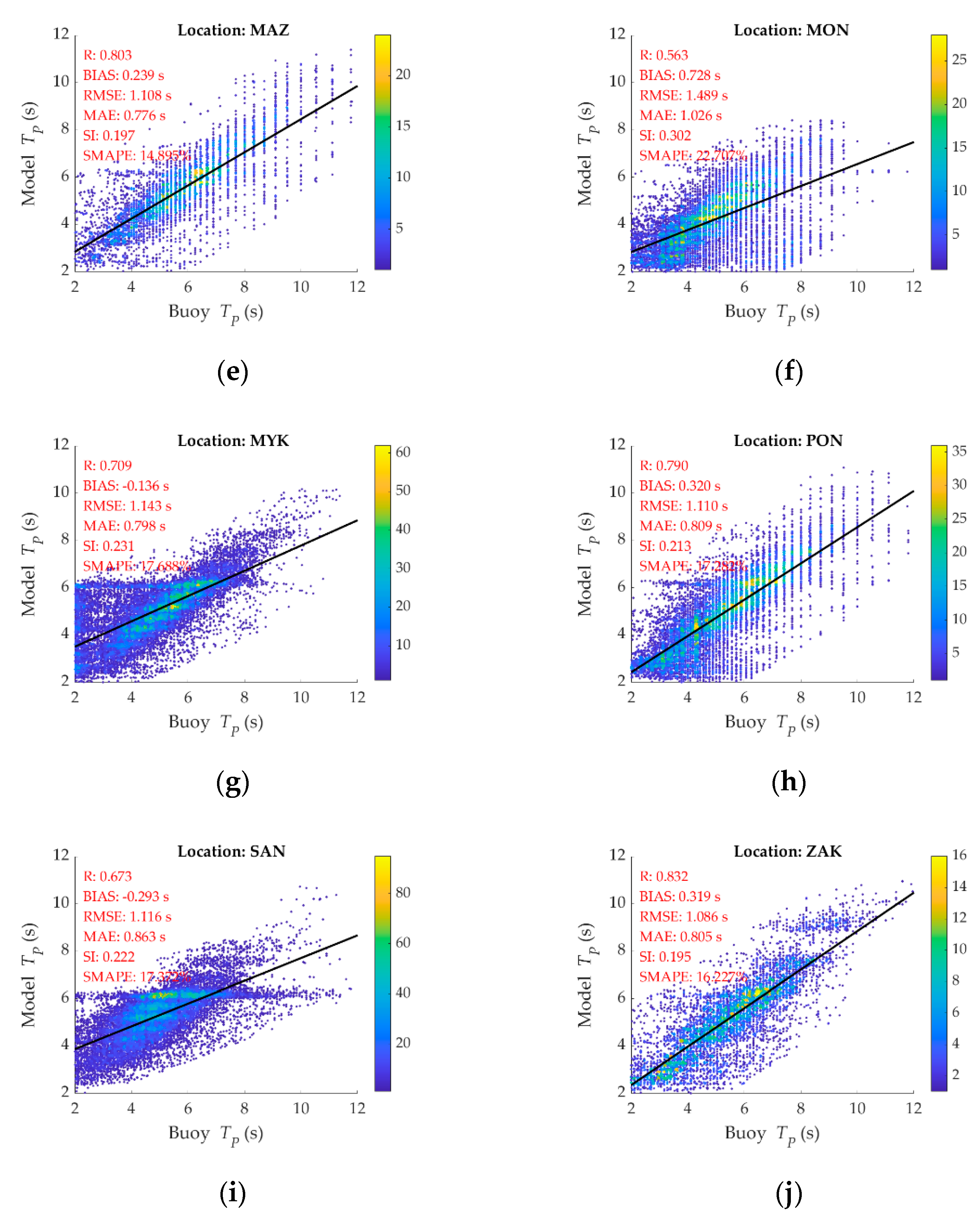
2.2. Evaluation
3. Theoretical Background and Methodology
3.1. Brief Theoretical Background for Wave Parameters
3.2. Theoretical Background for Block Maxima Method in Extreme Value Theory
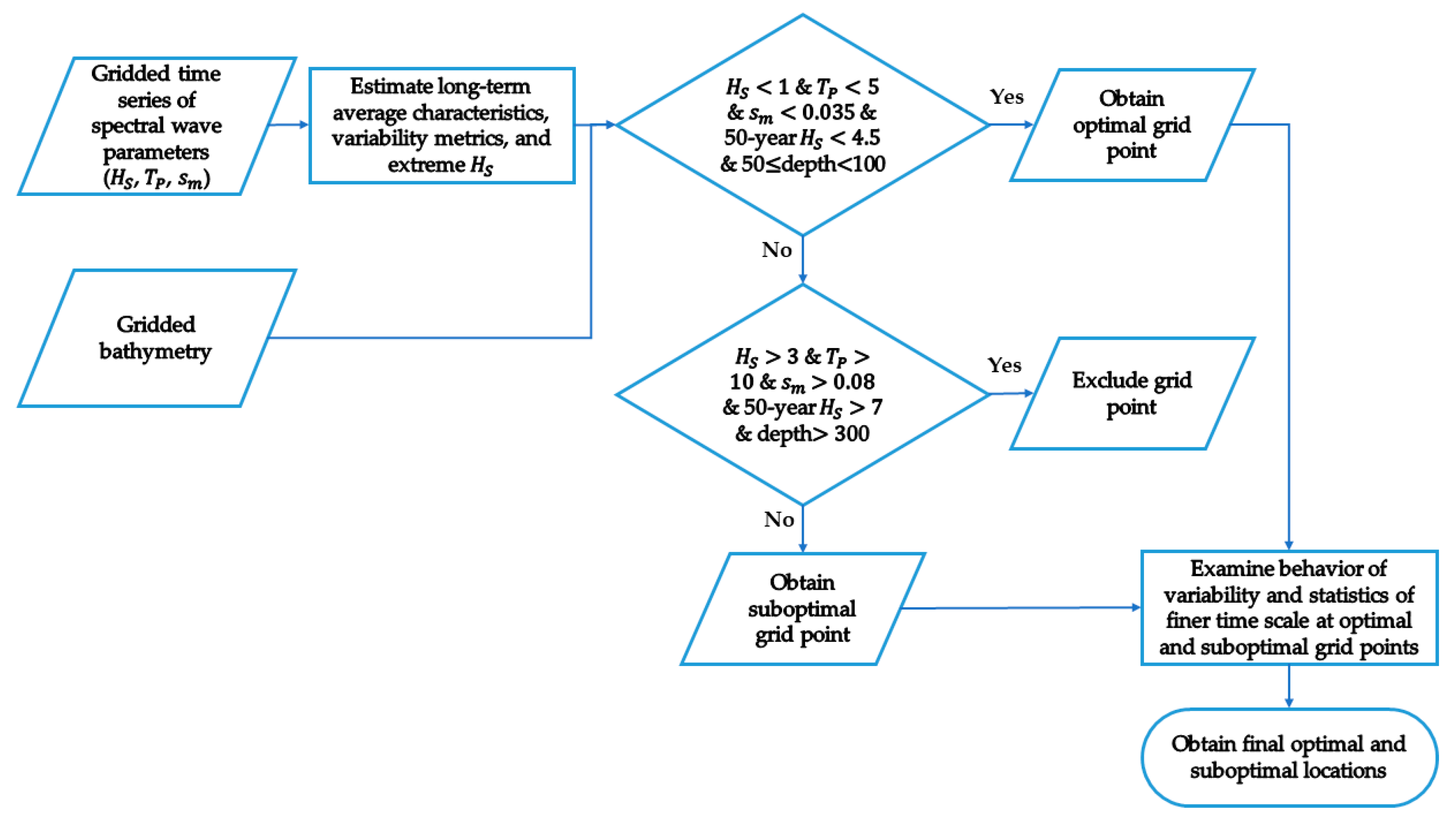
3.3. Methodology for the Identification of Favourite Sites for Offshore Aquaculture
4. Results
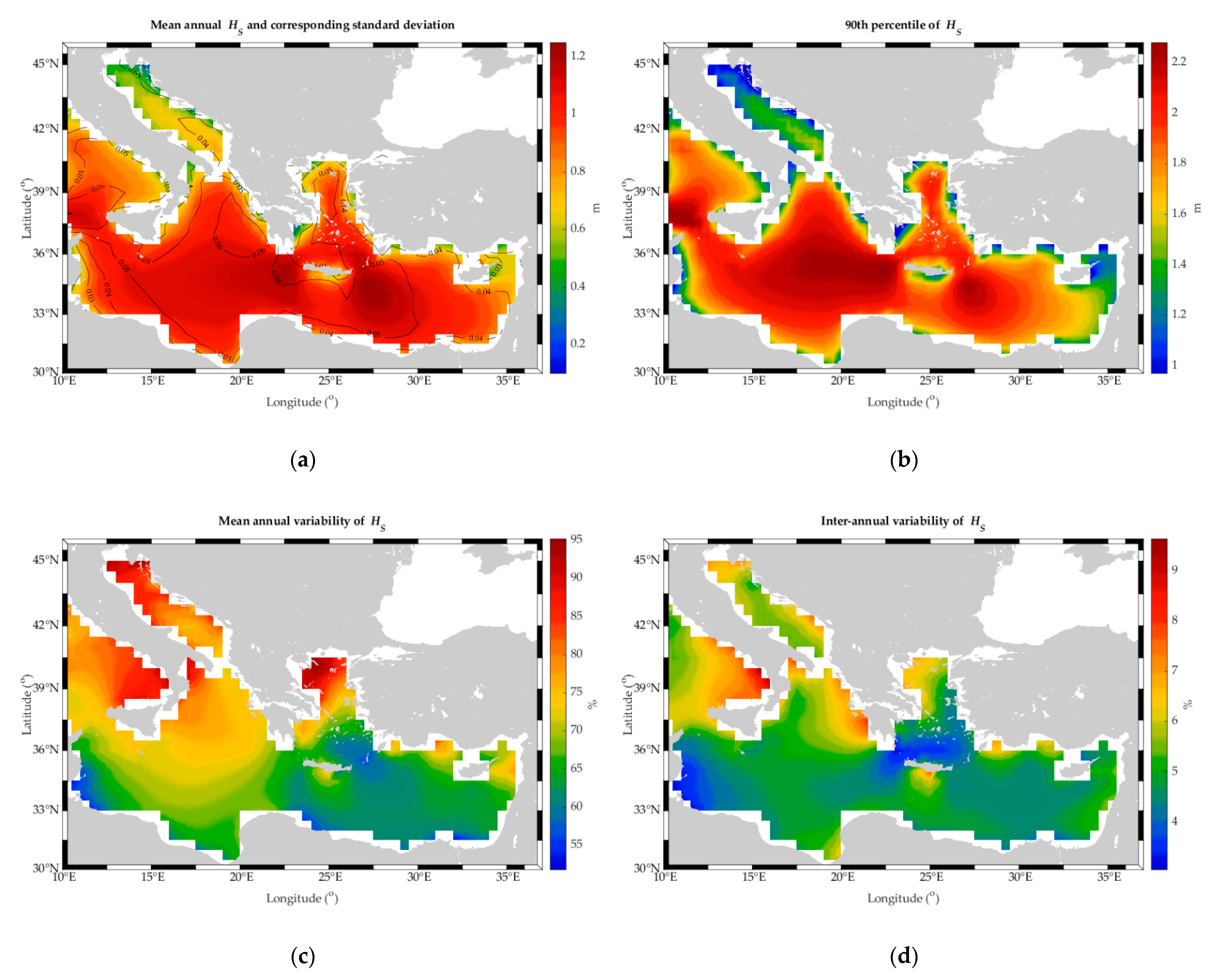
4.1. Wave Climate
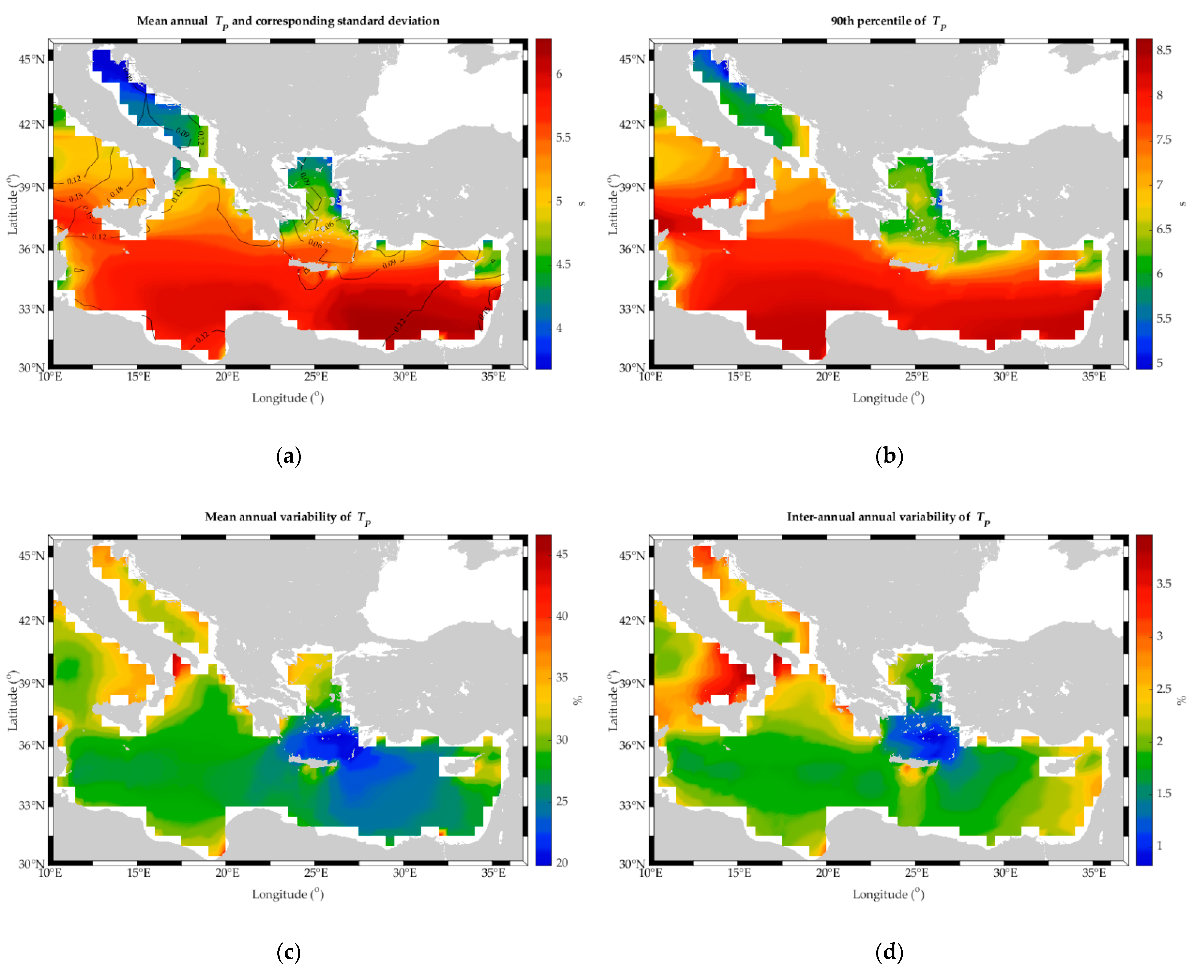
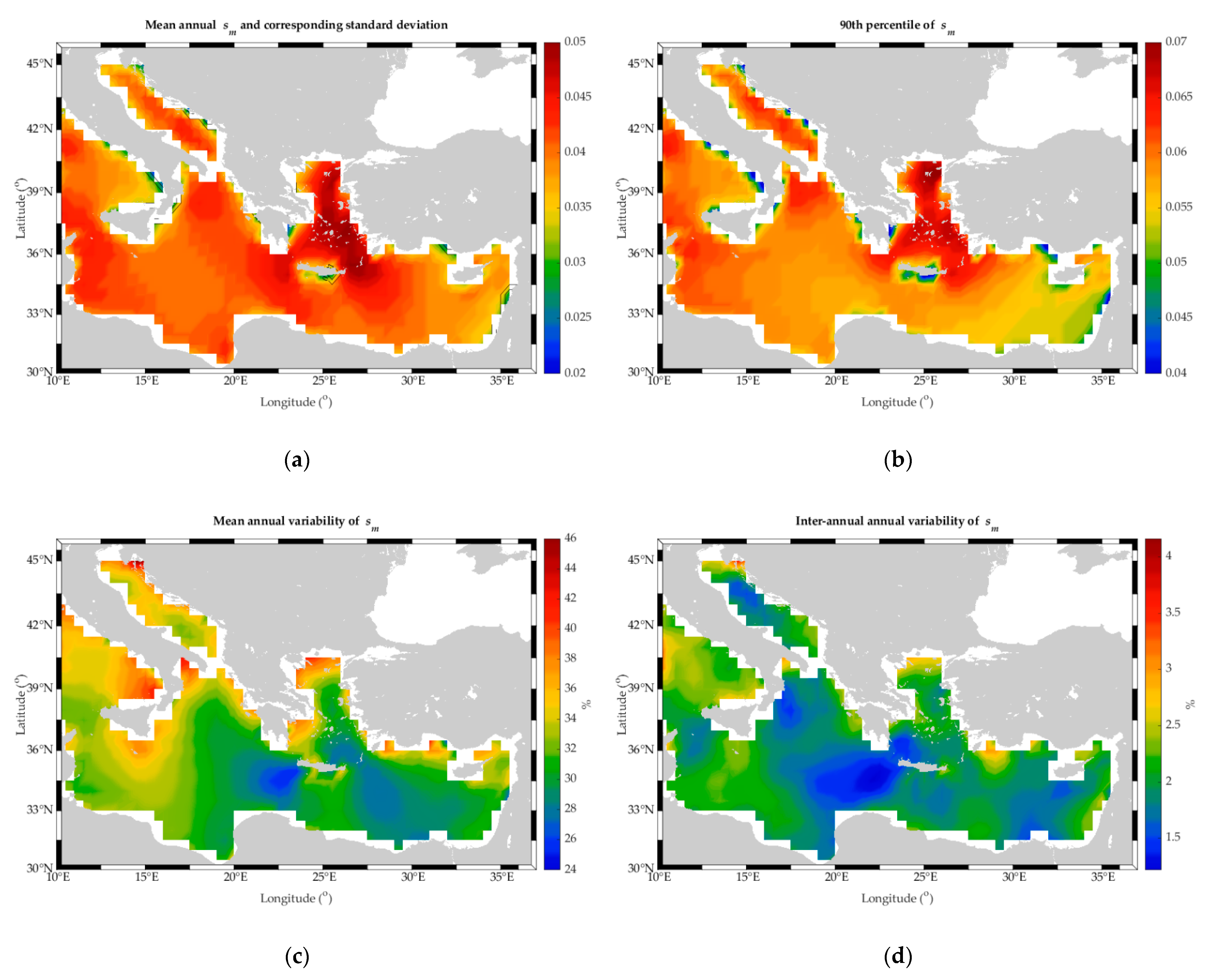
4.1.1. Annual and Hourly Analysis
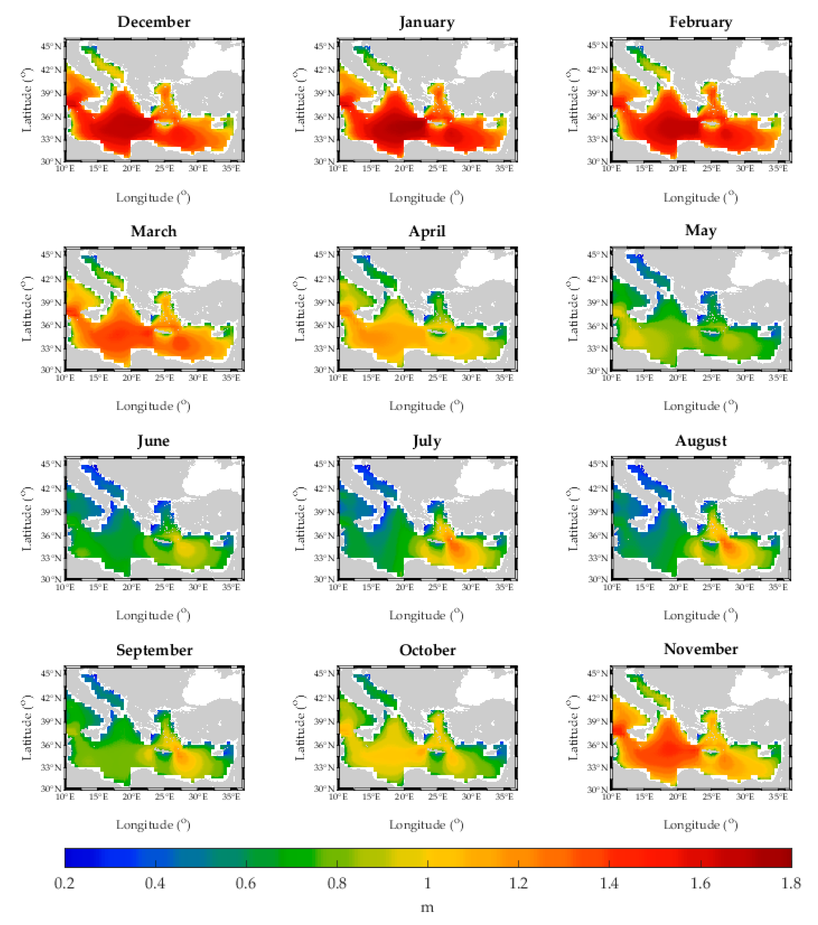
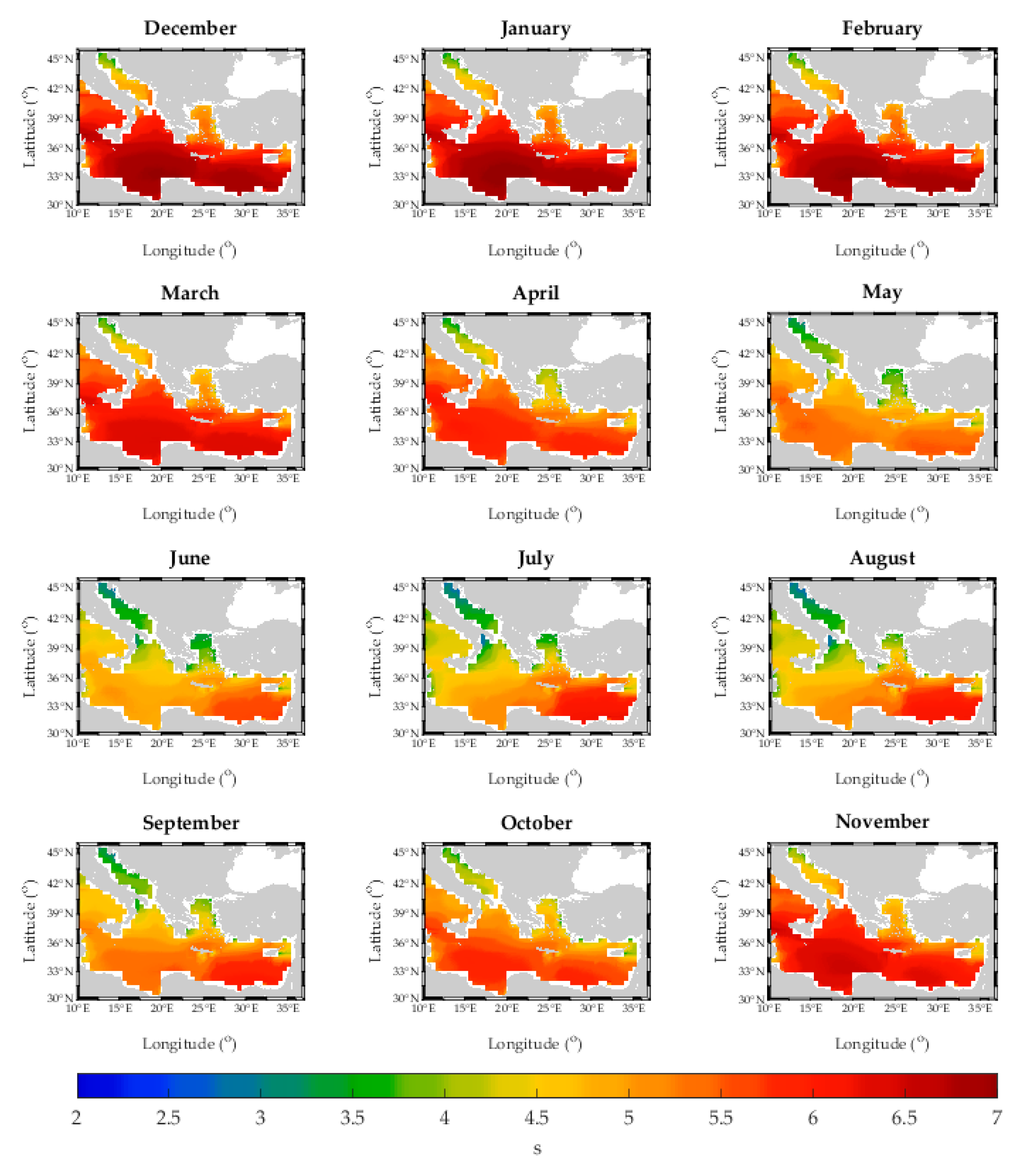
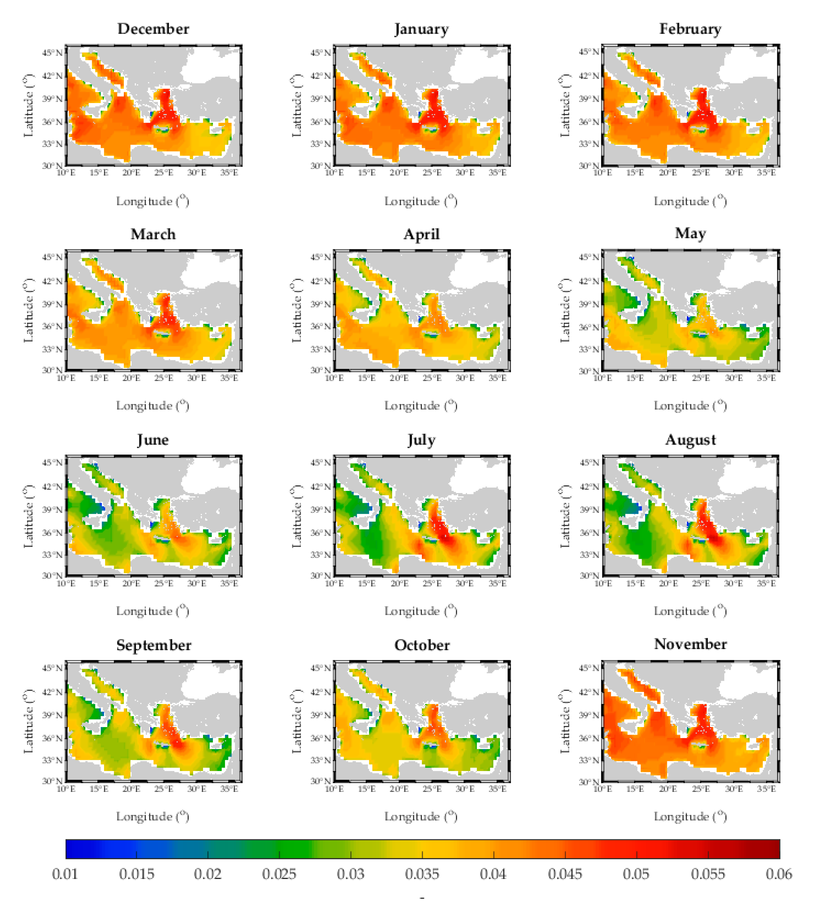
4.1.2. Monthly Analysis
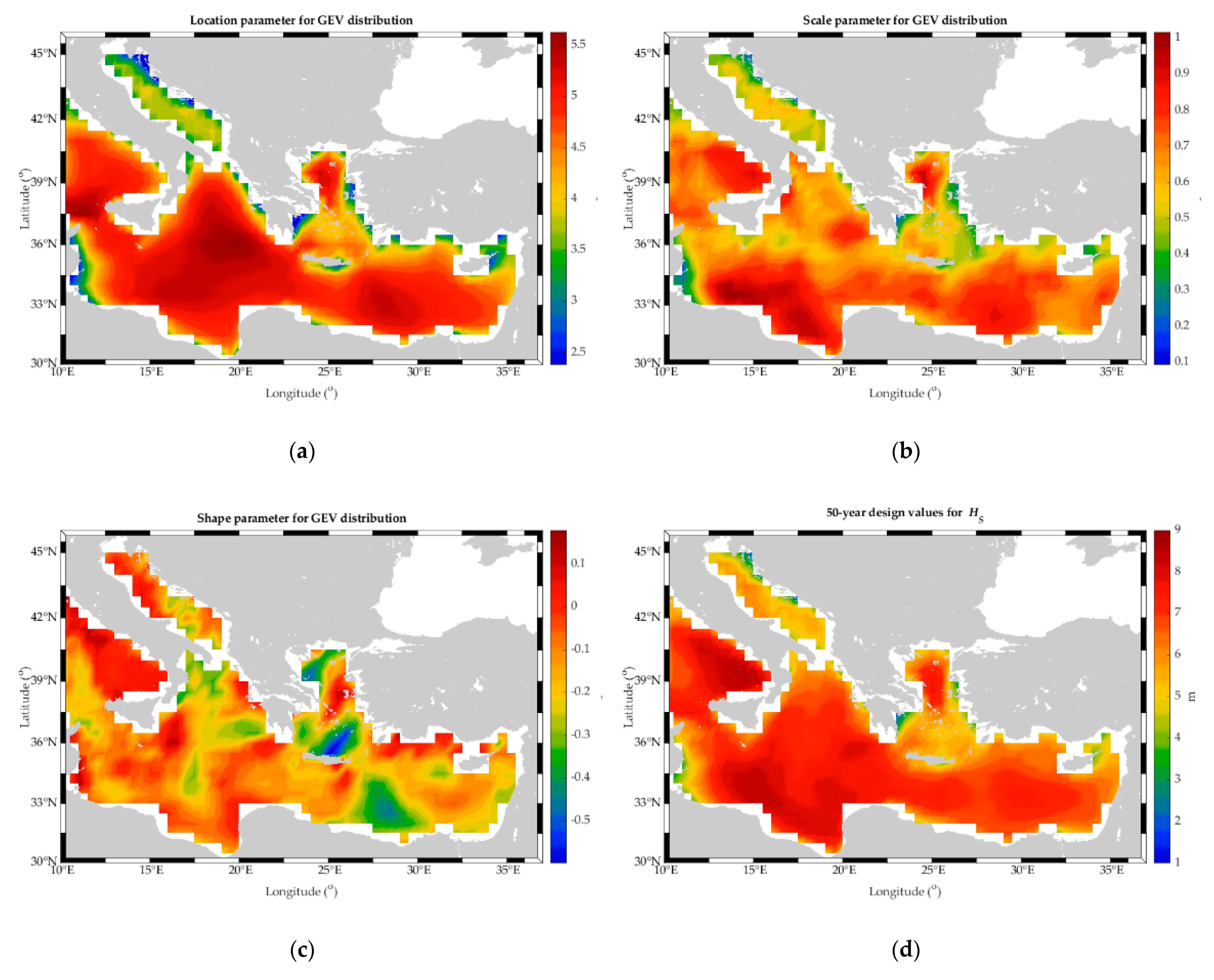
4.1.3. Extreme Value Analysis of Significant Wave Heights
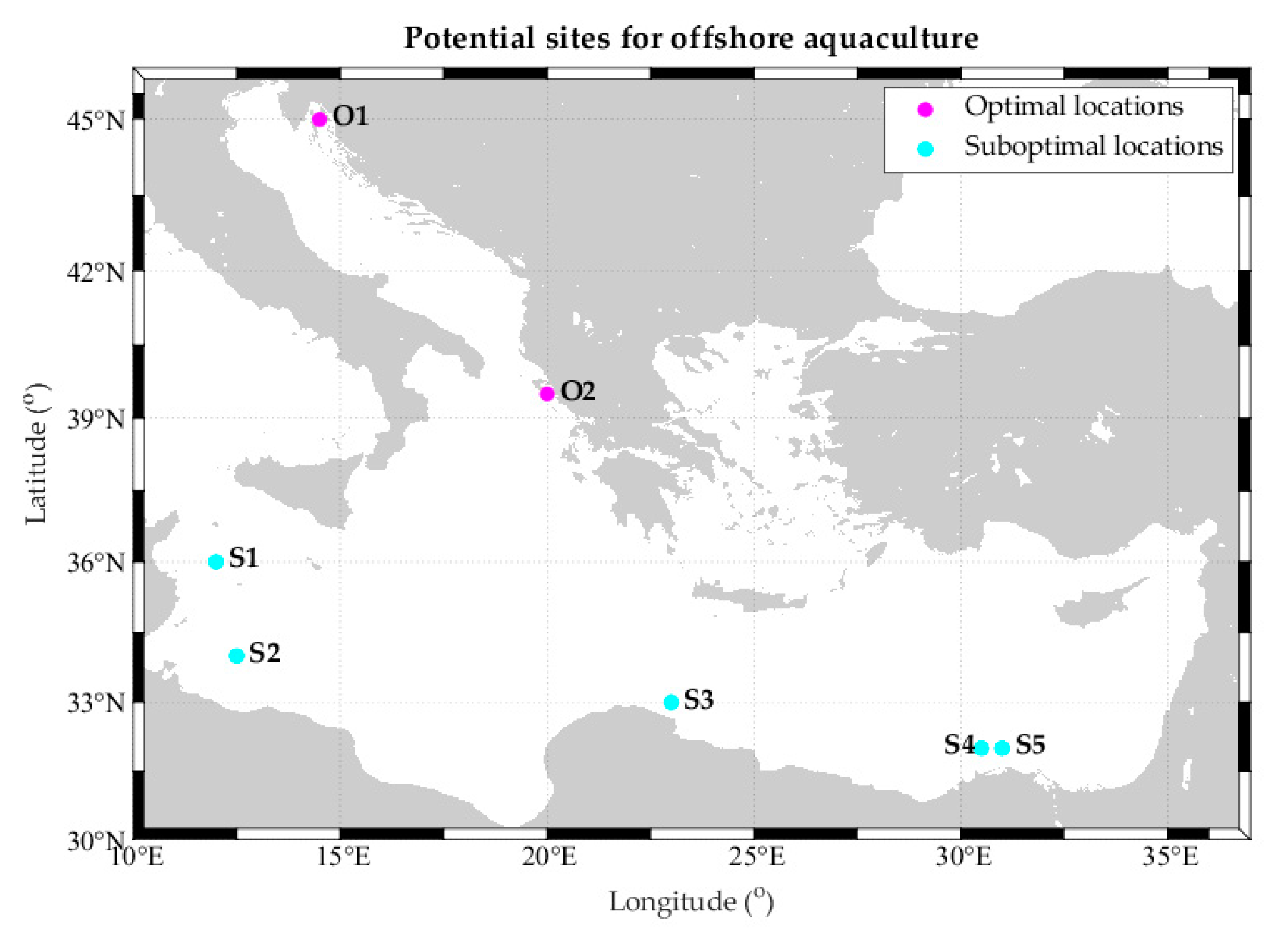
4.2. Identification of Sites Based on Wave Climate and Bathymetry
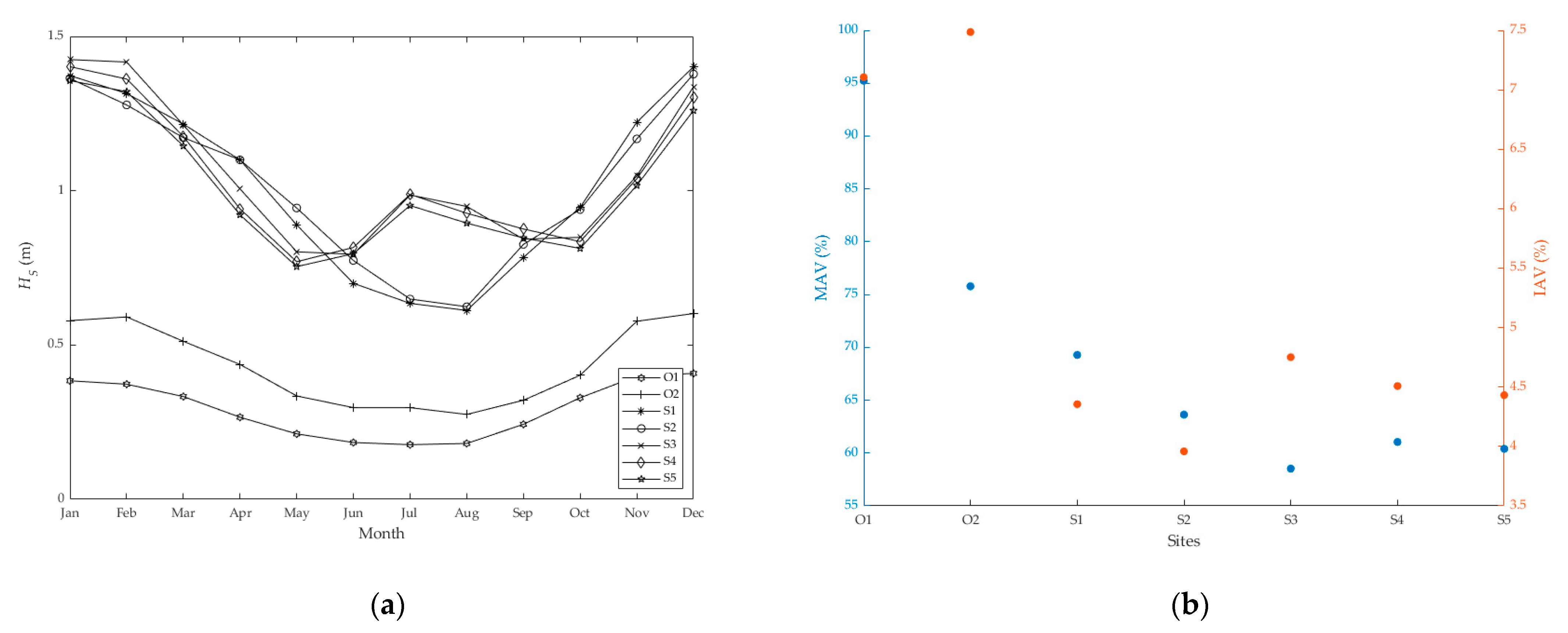
- For the optimal sites, O1 site is characterized by a very mild wave climate for all months due to its sheltered location, with values below 0.41 m. For both sites, MAV and IAV values are considered rather high compared to the other areas of the examined basin.
- For the suboptimal sites, S3, S4, and S5 sites (all located in the southern part of the examined basin) present a smaller range of values (<0.63 m) compared to the other two suboptimal sites; the former sites have higher mean monthly values during summer and September, and lower values during April, May, October, November, and December. All sites present lower variability values compared to the optimal locations, with S2 and S3 having the lowest IAV and MAV values, respectively.
5. Discussion
6. Conclusions
- The thorough evaluation of the ERA5 wave model data showed good agreement with buoy measurements in the basin of interest.
- Wave analysis in extended sea areas for site selection purposes should be based on long-term data and include average statistics, variability measures and extreme values.
- Apart from common sea state variables, wave steepness is also recommended to be embedded in relevant studies as an additional variable affecting the design of offshore fish cages.
- The proposed methodology is a step forward in supporting the sustainable development of offshore aquaculture in the Mediterranean Sea and elsewhere. It can also be considered as a precursor of a more holistic approach, incorporating more parameters that influence the site selection procedure.
Author Contributions
Funding
Data Availability Statement
Acknowledgments
Conflicts of Interest
References
- Scientific Technical and Economic Committee for Fisheries. The EU Aquaculture Sector—Economic Report 2020 (STECF-20-12, JRC124931); Publications Office of the European Union: Luxembourg, 2021; pp. 306–307. Available online: https://op.europa.eu/en/publication-detail/-/publication/1939335e-a893-11eb-9585-01aa75ed71a1/language-en (accessed on 12 October 2021).
- Campbell, B.; Pauly, D. Mariculture: A global analysis of production trends since 1950. Mar. Policy 2013, 39, 94–100. [Google Scholar] [CrossRef]
- Martins, C.; Eding, E.; Verdegem, M.; Heinsbroek, L.; Schneider, O.; Blancheton, J.; D’Orbcastel, E.R.; Verreth, J. New developments in recirculating aquaculture systems in Europe: A perspective on environmental sustainability. Aquac. Eng. 2010, 43, 83–93. [Google Scholar] [CrossRef] [Green Version]
- Watson, R.; Green, B.S.; Tracey, S.R.; Farmery, A.; Pitcher, T.J. Provenance of global seafood. Fish Fish. 2015, 17, 585–595. [Google Scholar] [CrossRef]
- Price, C.; Black, K.; Hargrave, B.; Morris, J. Marine cage culture and the environment: Effects on water quality and primary production. Aquac. Environ. Interact. 2015, 6, 151–174. [Google Scholar] [CrossRef] [Green Version]
- Holmer, M. Environmental issues of fish farming in offshore waters: Perspectives, concerns and research needs. Aquac. Environ. Interact. 2010, 1, 57–70. [Google Scholar] [CrossRef] [Green Version]
- Vizzini, S.; Mazzola, A. The effects of anthropogenic organic matter inputs on stable carbon and nitrogen isotopes in organisms from different trophic levels in a southern Mediterranean coastal area. Sci. Total Environ. 2006, 368, 723–731. [Google Scholar] [CrossRef] [PubMed]
- Stickney, R.R.; McVey, J.P. Responsible Marine Aquaculture; Cabi Publishing: Oxfordshire, UK, 2002; p. 391. [Google Scholar]
- Froehlich, H.E.; Smith, A.; Gentry, R.R.; Halpern, B.S. Offshore Aquaculture: I Know It When I See It. Front. Mar. Sci. 2017, 4, e154. [Google Scholar] [CrossRef]
- Gentry, R.R.; Froehlich, H.E.; Grimm, D.; Kareiva, P.; Parke, M.; Rust, M.; Gaines, S.D.; Halpern, B.S. Mapping the global potential for marine aquaculture. Nat. Ecol. Evol. 2017, 1, 1317–1324. [Google Scholar] [CrossRef]
- FAO. A Global Assessment of Offshore Mariculture Potential from a Spatial Perspective, in FAO; Fisheries and Aquaculture Technical Paper; FAO: Rome, Italy, 2013. [Google Scholar]
- Cairns, J.; Linfoot, B.T. Some considerations in the structural engineering of sea-cages for aquaculture. In Engineering for Offshore Fish; Osborn, H.D., Eadie, H.S., Funnell, C., Kuo, C., Linfoot, B.T., Eds.; Thomas Telford: Telford, UK, 1990; pp. 63–77. [Google Scholar]
- Mohd Atif, S. Offshore Aquaculture in India: Site Considerations and Challenges in Indian Coastal Conditions. Oceanogr. Fish Open Access. J. 2018, 7, 555714. [Google Scholar]
- Neary, V.S.; Ahn, S.; Seng, B.E.; Allahdadi, M.N.; Wang, T.; Yang, Z.; He, R. Characterization of Extreme Wave Conditions for Wave Energy Converter Design and Project Risk Assessment. J. Mar. Sci. Eng. 2020, 8, 289. [Google Scholar] [CrossRef] [Green Version]
- Hiles, C.E.; Robertson, B.; Buckham, B.J. Extreme wave statistical methods and implications for coastal analyses. Estuar. Coast. Shelf Sci. 2019, 223, 50–60. [Google Scholar] [CrossRef]
- Jonathan, P.; Ewans, K. Statistical modelling of extreme ocean environments for marine design: A review. Ocean Eng. 2013, 62, 91–109. [Google Scholar] [CrossRef]
- Goda, Y. Random Seas and Design of Maritime Structures, 2nd ed.; Advanced Series on Ocean Engineering; World Scientific Publishing Co. Pte. Ltd.: Singapore, 2000; p. 443. [Google Scholar]
- Pérez, O.; Telfer, T.; Ross, L. On the calculation of wave climate for offshore cage culture site selection: A case study in Tenerife (Canary Islands). Aquac. Eng. 2003, 29, 1–21. [Google Scholar] [CrossRef]
- Benetti, D.D.; Benetti, G.I.; Rivera, J.A.; Sardenberg, B.; O’Hanlon, B. Site Selection Criteria for Open Ocean Aquaculture. Mar. Technol. Soc. J. 2010, 44, 22–35. [Google Scholar] [CrossRef]
- Longdill, P.C.; Healy, T.R.; Black, K.P. An integrated GIS approach for sustainable aquaculture management area site selection. Ocean Coast. Manag. 2008, 51, 612–624. [Google Scholar] [CrossRef]
- Szuster, W.B.; Albasri, H. Site selection for Grouper Mariculture in Indonesia. Int. J. Fish. Aquac. 2010, 2, 87–92. [Google Scholar]
- Micael, J.; Costa, A.; Aguiar, P.; Medeiros, A.; Calado, H. Geographic Information System in a Multi-Criteria Tool for Mariculture Site Selection. Coast. Manag. 2015, 43, 52–66. [Google Scholar] [CrossRef]
- Stelzenmüller, V. Aquaculture Site-Selection and Marine Spatial Planning: The Roles of GIS-Based Tools and Models. In Aquaculture Perspective of Multi-Use Sites in the Open Ocean: The Untapped Potential for Marine Resources in the Anthropocene; Buck, B.H., Langan, R., Eds.; Springer International Publishing: Cham, Switzerland, 2017; pp. 131–148. [Google Scholar]
- Junaidi, M.; Scabra, A.R. Mariculture site selection based on environ-mental parameters in Tanjung and Gangga Sub-District, North Lombok. In Proceedings of the 1st International Conference and Workshop on Bioscience and Biotechnology for Human Health and Prosperity, Mataram, Indonesia, 28–30 November 2018; pp. 233–251. [Google Scholar]
- Vianna, L.F.d.N.; Filho, J.B. Spatial analysis for site selection in marine aquaculture: An ecosystem approach applied to Baía Sul, Santa Catarina, Brazil. Aquaculture 2018, 489, 162–174. [Google Scholar] [CrossRef]
- Divu, D.N.; Mojjada, S.K.; Pokkathappada, A.A.; Sukhdhane, K.; Menon, M.; Tade, M.S.; Bhint, H.M.; Gopalakrishnan, A. Decision-making framework for identifying best suitable mariculture sites along north east coast of Arabian Sea, India: A preliminary GIS-MCE based modelling approach. J. Clean. Prod. 2021, 284, 124760. [Google Scholar] [CrossRef]
- Porporato, E.M.D.; Pastres, R.; Brigolin, D. Site Suitability for Finfish Marine Aquaculture in the Central Mediterranean Sea. Front. Mar. Sci. 2020, 6, 772. [Google Scholar] [CrossRef] [Green Version]
- Zikra, M.; Armono, H.D.; Mahaputra, B. Site selection of aquaculture location in Indonesia Sea. Ecol. Environ. Conserv. 2020, 26, S8–S17. [Google Scholar]
- FAO. The State of the Mediterranean and Black Sea Fisheries Series, 2nd ed.; FAO: Rome, Italy, 2018; p. 170. [Google Scholar]
- Haver, S. Design of offshore structures: Impact of the possible existence of freak waves. In Proceedings of the 14th Aha Hulikoá Hawaiian Winter Workshop on Rogue Waves, Hawaii, HI, USA, 25–28 January 2005; pp. 161–175. [Google Scholar]
- Bitner-Gregersen, E.M.; Toffoli, A. Wave Steepness and Rogue Waves in the Changing Climate in the North Atlantic. In Proceedings of the 2015 34th International Conference on Ocean, Offshore and Arctic Engineering, St. John’s, NL, Canada, 31 May–5 June 2015. [Google Scholar]
- Hersbach, H.; Bell, B.; Berrisford, P.; Hirahara, S.; Horányi, A.; Muñoz-Sabater, J.; Nicolas, J.; Peubey, C.; Radu, R.; Schepers, D.; et al. The ERA5 global reanalysis. Q. J. R. Meteorol. Soc. 2020, 146, 1999–2049. [Google Scholar] [CrossRef]
- Hoffmann, L.; Günther, G.; Li, D.; Stein, O.; Wu, X.; Griessbach, S.; Heng, Y.; Konopka, P.; Müller, R.; Vogel, B. From ERA-Interim to ERA5: The considerable impact of ECMWF’s next-generation reanalysis on Lagrangian transport simulations. Atmos. Chem. Phys. 2019, 19, 3097–3124. [Google Scholar] [CrossRef] [Green Version]
- Mahmoodi, K.; Ghassemi, H.; Razminia, A. Temporal and spatial characteristics of wave energy in the Persian Gulf based on the ERA5 reanalysis dataset. Energy 2019, 187, 115991. [Google Scholar] [CrossRef]
- Naseef, T.M.; Kumar, V.S. Climatology and trends of the Indian Ocean surface waves based on 39-year long ERA5 reanalysis data. Int. J. Clim. 2020, 40, 979–1006. [Google Scholar] [CrossRef]
- Bruno, M.F.; Molfetta, M.G.; Totaro, V.; Mossa, M. Performance Assessment of ERA5 Wave Data in a Swell Dominated Region. J. Mar. Sci. Eng. 2020, 8, 214. [Google Scholar] [CrossRef] [Green Version]
- Hisaki, Y. Intercomparison of Assimilated Coastal Wave Data in the Northwestern Pacific Area. J. Mar. Sci. Eng. 2020, 8, 579. [Google Scholar] [CrossRef]
- Aguinis, H.; Gottfredson, R.K.; Joo, H. Best-Practice Recommendations for Defining, Identifying, and Handling Outliers. Organ. Res. Methods 2013, 16, 270–301. [Google Scholar] [CrossRef]
- Soukissian, T.; Karathanasi, F.; Axaopoulos, P. Satellite-Based Offshore Wind Resource Assessment in the Mediterranean Sea. IEEE J. Ocean. Eng. 2017, 42, 73–86. [Google Scholar] [CrossRef]
- Soukissian, T.; Papadopoulos, A.; Skrimizeas, P.; Karathanasi, F.; Axaopoulos, P.; Avgoustoglou, E.; Kyriakidou, H.; Tsalis, C.; Voudouri, A.; Gofa, F.; et al. Assessment of offshore wind power potential in the Aegean and Ionian Seas based on high-resolution hindcast model results. AIMS Energy 2017, 5, 268–289. [Google Scholar] [CrossRef]
- Lavidas, G.; Venugopal, V. A 35 year high-resolution wave atlas for nearshore energy production and economics at the Aegean Sea. Renew. Energy 2017, 103, 401–417. [Google Scholar] [CrossRef] [Green Version]
- Mendes, D.; Oliveira, T.C. Deep-water spectral wave steepness offshore mainland Portugal. Ocean Eng. 2021, 236, 109548. [Google Scholar] [CrossRef]
- Myrhaug, D. Some probabilistic properties of deep water wave steepness. Oceanologia 2018, 60, 187–192. [Google Scholar] [CrossRef]
- Bücher, A.; Zhou, C. A Horse Race between the Block Maxima Method and the Peak–over–Threshold Approach. Stat. Sci. 2021, 36, 360–378. [Google Scholar] [CrossRef]
- Coles, S. An Introduction to Statistical Modeling of Extreme Values; Springer: London, UK, 2001. [Google Scholar]
- Fisher, R.A.; Tippett, L.H.C. Limiting forms of the frequency distribution of the largest or smallest member of a sample. In Mathematical Proceedings of the Cambridge Philosophical Society; Cambridge University Press: Cambridge, UK, 1928; Volume 24, pp. 180–190. [Google Scholar]
- Gnedenko, B. Sur La Distribution Limite Du Terme Maximum D’Une Serie Aleatoire. Ann. Math. 1943, 44, 423. [Google Scholar] [CrossRef]
- von Mises, R. La distribution de la plus grande de n valeurs. Rev. Math. Union Interbalcanique 1936, 1, 141–160. [Google Scholar]
- Soukissian, T.H.; Tsalis, C. The effect of the generalized extreme value distribution parameter estimation methods in extreme wind speed prediction. Nat. Hazards 2015, 78, 1777–1809. [Google Scholar] [CrossRef]
- Soukissian, T.H.; Tsalis, C. Effects of parameter estimation method and sample size in metocean design conditions. Ocean Eng. 2018, 169, 19–37. [Google Scholar] [CrossRef]
- Hosking, J.R.M. L-Moments: Analysis and Estimation of Distributions Using Linear Combinations of Order Statistics. J. R. Stat. Soc. Ser. B Stat. Methodol. 1990, 52, 105–124. [Google Scholar] [CrossRef]
- Jackson, D.; Drumm, A.; Fredheim, A.; Lader, P.; Fernáandez Otero, R. Evaluation of the Promotion of Offshore Aquaculture through a Technology Platform (OATP), Report; Marine Institute: Galway, Ireland, 2011; Available online: https://oar.marine.ie/handle/10793/1086 (accessed on 15 October 2021).
- NS 9415; Floating Aquaculture Farms—Site Survey, Design, Execution and Use. Standards Norway: Lysaker, Norway, 2021; p. 140. Available online: https://www.standard.no/no/Nettbutikk/produktkatalogen/Produktpresentasjon/?ProductID=1367329 (accessed on 15 October 2021).
- NS 9415; Marine Fish Farms–Requirements for Site Survey, Risk Analyses, Design, Dimensioning, Production, Installation and Operation. Standards Norway: Lysaker, Norway, 2009; p. 108. Available online: https://www.standard.no/no/nettbutikk/produktkatalogen/produktpresentasjon/?ProductID=402400 (accessed on 15 October 2021).
- Yang, X.; Ramezani, R.; Utne, I.B.; Mosleh, A.; Lader, P.F. Operational limits for aquaculture operations from a risk and safety perspective. Reliab. Eng. Syst. Saf. 2020, 204, 107208. [Google Scholar] [CrossRef]
- Chu, Y.I.; Wang, C.; Park, J.; Lader, P. Review of cage and containment tank designs for offshore fish farming. Aquaculture 2020, 519, 734928. [Google Scholar] [CrossRef]
- Cifuentes Salazar, C.A. Dynamic Analysis of Cage Systems under Waves and Current for Offshore Aquaculture; Texas A&M University: College Station, TX, USA, 2016; p. 244. [Google Scholar]
- Lovatelli, A.; Aguilar-Manjarrez, J.; Soto, D. Expanding Mariculture Farther Offshore: Technical, Environmental, Spatial and Governance Challenges. In FAO Technical Workshop; FAO: Orbetello, Italy, 2013. [Google Scholar]
- EMODnet Bathymetry Consortium. EMODnet Digital Bathymetry (DTM). 2016; Available online: https://doi.org/10.12770/c7b53704-999d-4721-b1a3-04ec60c87238 (accessed on 25 October 2021).
- Soukissian, T.; Karathanasi, F.; Axaopoulos, P.; Voukouvalas, E.; Kotroni, V. Offshore wind climate analysis and variability in the Mediterranean Sea. Int. J. Clim. 2018, 38, 384–402. [Google Scholar] [CrossRef]
- Wang, T.; Yang, Z.; Wu, W.-C.; Grear, M. A Sensitivity Analysis of the Wind Forcing Effect on the Accuracy of Large-Wave Hindcasting. J. Mar. Sci. Eng. 2018, 6, 139. [Google Scholar] [CrossRef] [Green Version]
- Vanem, E. Uncertainties in extreme value modelling of wave data in a climate change perspective. J. Ocean Eng. Mar. Energy 2015, 1, 339–359. [Google Scholar] [CrossRef] [Green Version]


| Location Name | Longitude (deg) | Latitude (deg) | Depth (m) | Distance from Closest Grid Point (km) | Period |
|---|---|---|---|---|---|
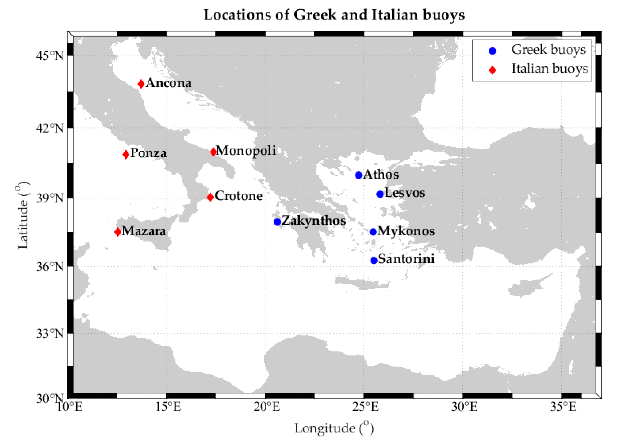
| Ancona (ANC) | 13.719 | 43.825 | 71 | 26.3 | June 2013–November 2014 |
| Athos (ATH) | 24.729 | 39.975 | 228 | 20.3 | May 2000–June 2021 |
| Crotone (CRO) | 17.220 | 39.024 | 7 | 24.8 | June 2013–December 2014 |
| Lesvos (LES) | 25.807 | 39.156 | 122 | 24.2 | January 2001–July 2012 |
| Mazara (MAZ) | 12.533 | 37.518 | 87 | 3.6 | August 2013–October 2014 |
| Monopoli (MON) | 17.378 | 40.975 | 79 | 10.7 | June 2013–January 2015 |
| Mykonos (MYK) | 25.460 | 37.519 | 105 | 4.3 | January 2001–June 2020 |
| Ponza (PON) | 12.950 | 40.867 | 17 | 15.4 | June 2013–January 2015 |
| Santorini (SAN) | 25.501 | 36.262 | 271 | 26.4 | March 2001–March 2011 |
| Zakynthos (ZAK) | 20.604 | 37.956 | 259 | 10.5 | November 2007–January 2012 |
| Location | Source | m | |||||||
|---|---|---|---|---|---|---|---|---|---|
| ANC | Buoy | 2331 | 0.93 | 0.75 | 0.07 | 5.01 | 80.05 | 1.82 | 7.29 |
| Model | 0.72 | 0.64 | 0.04 | 5.19 | 89.54 | 2.40 | 11.21 | ||
| ATH | Buoy | 29,114 | 0.86 | 0.74 | 0.04 | 5.79 | 85.65 | 1.92 | 7.00 |
| Model | 0.78 | 0.70 | 0.04 | 5.80 | 89.44 | 0.74 | 7.65 | ||
| CRO | Buoy | 11,766 | 0.66 | 0.56 | 0.04 | 6.46 | 85.05 | 2.87 | 18.24 |
| Model | 0.57 | 0.45 | 0.05 | 4.79 | 80.03 | 2.58 | 14.13 | ||
| LES | Buoy | 21,193 | 0.77 | 0.52 | 0.00 | 4.81 | 67.85 | 1.57 | 6.77 |
| Model | 0.64 | 0.47 | 0.04 | 3.69 | 73.24 | 1.73 | 7.16 | ||
| MAZ | Buoy | 5543 | 0.79 | 0.54 | 0.03 | 4.58 | 69.41 | 1.88 | 8.02 |
| Model | 0.75 | 0.49 | 0.09 | 3.88 | 65.34 | 2.11 | 9.34 | ||
| MON | Buoy | 12,680 | 0.65 | 0.48 | 0.03 | 3.71 | 74.41 | 1.90 | 8.39 |
| Model | 0.58 | 0.43 | 0.04 | 3.51 | 75.05 | 1.78 | 7.39 | ||
| MYK | Buoy | 23,849 | 1.03 | 0.75 | 0.05 | 5.76 | 73.15 | 1.11 | 4.31 |
| Model | 1.01 | 0.65 | 0.07 | 5.30 | 64.63 | 1.12 | 4.80 | ||
| PON | Buoy | 12,211 | 0.81 | 0.66 | 0.04 | 4.76 | 81.84 | 1.70 | 6.13 |
| Model | 0.66 | 0.54 | 0.06 | 3.73 | 81.32 | 1.84 | 6.80 | ||
| SAN | Buoy | 19,501 | 0.91 | 0.55 | 0.01 | 4.92 | 60.57 | 1.47 | 6.09 |
| Model | 1.03 | 0.60 | 0.05 | 4.51 | 58.03 | 1.06 | 4.29 | ||
| ZAK | Buoy | 7228 | 0.91 | 0.62 | 0.08 | 5.77 | 67.73 | 1.76 | 7.80 |
| Model | 0.90 | 0.64 | 0.06 | 5.57 | 71.35 | 1.48 | 6.09 |
| Location | Source | m | max | CV | |||||
|---|---|---|---|---|---|---|---|---|---|
| ANC | Buoy | 2305 | 4.93 | 1.79 | 2.00 | 10.00 | 36.28 | 0.46 | 2.35 |
| Model | 4.46 | 1.56 | 1.83 | 9.24 | 35.04 | 0.57 | 2.54 | ||
| ATH | Buoy | 26,063 | 4.65 | 1.42 | 1.99 | 11.01 | 30.56 | 0.42 | 3.00 |
| Model | 4.40 | 1.39 | 1.83 | 9.83 | 31.61 | 0.45 | 2.84 | ||
| CRO | Buoy | 11,719 | 4.99 | 1.67 | 2.00 | 12.50 | 33.53 | 0.63 | 3.29 |
| Model | 4.78 | 1.60 | 1.83 | 11.17 | 33.43 | 0.40 | 2.78 | ||
| LES | Buoy | 19,896 | 4.57 | 1.31 | 2.01 | 9.84 | 28.72 | 0.31 | 2.94 |
| Model | 4.34 | 1.22 | 1.83 | 9.29 | 27.98 | 0.42 | 3.00 | ||
| MAZ | Buoy | 5461 | 5.63 | 1.80 | 2.00 | 12.50 | 31.97 | 0.49 | 3.12 |
| Model | 5.40 | 1.57 | 1.83 | 11.39 | 29.17 | 0.52 | 3.49 | ||
| MON | Buoy | 12,707 | 4.93 | 1.50 | 2.00 | 11.76 | 30.40 | 0.51 | 3.07 |
| Model | 4.20 | 1.24 | 1.83 | 8.42 | 29.41 | 0.44 | 2.73 | ||
| MYK | Buoy | 19,949 | 4.95 | 1.61 | 2.01 | 11.37 | 32.43 | 0.17 | 2.79 |
| Model | 5.09 | 1.21 | 1.83 | 10.16 | 23.79 | 0.03 | 3.25 | ||
| PON | Buoy | 12,076 | 5.21 | 1.66 | 2.00 | 11.80 | 31.88 | 0.55 | 3.11 |
| Model | 4.89 | 1.61 | 1.83 | 11.08 | 32.98 | 0.36 | 2.66 | ||
| SAN | Buoy | 18,667 | 5.04 | 1.45 | 2.01 | 12.66 | 28.86 | 0.68 | 4.10 |
| Model | 5.33 | 1.04 | 2.04 | 12.05 | 19.43 | −0.10 | 3.64 | ||
| ZAK | Buoy | 6367 | 5.57 | 1.81 | 1.99 | 12.30 | 32.47 | 0.25 | 2.76 |
| Model | 5.26 | 1.77 | 1.93 | 11.33 | 33.61 | 0.41 | 2.83 |
| Parameter | Optimal | Suboptimal |
|---|---|---|
| (m) | <1 | [1, 3) |
| (s) | <5 | [5, 10) |
| (-) | <0.035 | [0.035, 0.08) |
| 50-year return period (m) | <4.5 | [4.5, 7) |
| Water depth (m) | [50, 100) | [100, 300) |
| Location | Lower 95% CI (m) | 50-Year Return Values (m) | Upper 95% CI (m) |
|---|---|---|---|
| O1 | 2.55 | 2.87 | 3.28 |
| O2 | 3.75 | 4.07 | 4.43 |
| S1 | 6.10 | 6.68 | 7.36 |
| S2 | 6.24 | 6.88 | 7.65 |
| S3 | 5.89 | 6.51 | 7.09 |
| S4 | 6.31 | 6.81 | 7.34 |
| S5 | 6.12 | 6.70 | 7.33 |
Publisher’s Note: MDPI stays neutral with regard to jurisdictional claims in published maps and institutional affiliations. |
© 2022 by the authors. Licensee MDPI, Basel, Switzerland. This article is an open access article distributed under the terms and conditions of the Creative Commons Attribution (CC BY) license (https://creativecommons.org/licenses/by/4.0/).
Share and Cite
Karathanasi, F.E.; Soukissian, T.H.; Hayes, D.R. Wave Analysis for Offshore Aquaculture Projects: A Case Study for the Eastern Mediterranean Sea. Climate 2022, 10, 2. https://doi.org/10.3390/cli10010002
Karathanasi FE, Soukissian TH, Hayes DR. Wave Analysis for Offshore Aquaculture Projects: A Case Study for the Eastern Mediterranean Sea. Climate. 2022; 10(1):2. https://doi.org/10.3390/cli10010002
Chicago/Turabian StyleKarathanasi, Flora E., Takvor H. Soukissian, and Daniel R. Hayes. 2022. "Wave Analysis for Offshore Aquaculture Projects: A Case Study for the Eastern Mediterranean Sea" Climate 10, no. 1: 2. https://doi.org/10.3390/cli10010002
APA StyleKarathanasi, F. E., Soukissian, T. H., & Hayes, D. R. (2022). Wave Analysis for Offshore Aquaculture Projects: A Case Study for the Eastern Mediterranean Sea. Climate, 10(1), 2. https://doi.org/10.3390/cli10010002