Article

Nonlinear Cointegrating Regression of the Earth’s Surface Mean Temperature Anomalies on Total Radiative Forcing

Energy Industry Research Group, Korea Energy Economics Institute, 405-11, Jongga-ro, Jung-gu, Ulsan 44543, Korea
Econometrics 2021, 9(1), 6; https://doi.org/10.3390/econometrics9010006
Submission received: 20 September 2020 / Revised: 30 January 2021 / Accepted: 2 February 2021 / Published: 8 February 2021
(This article belongs to the Collection Econometric Analysis of Climate Change)

Abstract

:
This study proposes a nonlinear cointegrating regression model based on the well-known energy balance climate model. Specifically, I investigate the nonlinear cointegrating regression of the mean of temperature anomaly distributions on total radiative forcing using estimated spatial distributions of temperature anomalies for the Globe, Northern Hemisphere, and Southern Hemisphere. Further, I provide two types of nonlinear response functions that map the total radiative forcing level to mean temperature anomalies. The proposed statistical model provides a climatological implication that spatially heterogenous warming effects play a significant role in identifying nonlinear climate sensitivity. Cointegration and specification tests are provided that support the existence of nonlinear effects of total radiative forcing.

1. Introduction

Over the past few decades, the observed global mean surface temperature has increased. With such an evident fact, global warming has received rapidly increasing attention during the past decades. Since all countries are involved in both the causes and consequences of this issue in a variety of complex ways, there have been worldwide debates on global warming among scientists and policymakers. To identify whether human activities are causing the recent rise in global mean temperature or whether their effects will have serious effects on the Earth, the detection and attribution of an anthropogenic influence on climate change has been studied extensively.
Climate sensitivity measures how much global warming will occur in response to a doubling of atmospheric concentration of carbon dioxide. Ultraviolet light from the Sun passes through greenhouse gases (GHG) such as carbon dioxide, water vapor, methane, nitrous oxide, and chlorofluorocarbons, and is absorbed by objects on the ground. Since GHG absorb the infrared radiation released by the objects and then reradiates it back to the surface of the Earth, global temperature is increasing as a result. We refer to this as the “Greenhouse Effect” (Hansen et al. 2011). It is well-known that GHG in the atmosphere have been consistently increasing due to human activity. Note that the atmospheric lifetime of carbon dioxide is currently estimated at 5–200 years (IPCC 2007). As a result of such accumulation, the stock of carbon dioxide in the atmosphere has increased by approximately 130 ppm over the last 270 years, from a range of between 275 and 285 ppm in the pre-industrial era to 410 ppm in 2018.
According to IPCC (2014), the global mean temperature on the surface of the Earth has increased by approximately 0.85 ° C since 1880 and “most of the observed warming over the last 50 years is likely to have been due to the increase in GHG emissions.” Scientists have attempted to estimate the effect of GHG, according to which doubling carbon dioxide concentration in the atmosphere (a forcing of 4 W/m 2 ) may increase the average global temperature by 1.5 to 4.5 ° C. To stress the serious impact of increasing global temperature, Stern (2008) states that, “around 10,000–12,000 years ago, temperatures were approximately 5 ° C lower than today, and ice sheets came down to latitudes just north of London and south of New York. As the ice melted and sea levels rose, England separated from the continent, rerouting much of the river flow. These magnitudes of temperature changes transform the planet”.
A time series analysis has been employed to test the anthropogenic global warming hypothesis. This hypothesis test has resulted in extensive controversy over the last two decades. The main argument relates to whether observing trends in temperature series and radiative forcing contain stochastic trends or deterministic trends with a structural break. During early years, Kaufmann et al. (2006a, 2006b, 2010, 2013) and Kaufmann and Stern (2002) had a breakthrough on the linear cointegration analysis between temperature series and radiative forcing variables by assuming they are integrated processes or difference stationary processes. Using Dynamic Ordinary Least Squares estimation, they concluded that the increase in global mean temperature can be associated with the change in radiative forcing variables. Such a linear cointegration analysis has also been investigated by Pretis (2020). He linked a two-component energy balance climate model of global mean temperature with a testable cointegrated Vector Autoregressive model.
Some econometricians cast doubt on their statistical rigor and challenged their empirical results (Gay-Garcia et al. 2009; Perron and Estrada 2012; Estrada et al. 2013a, 2013b; Estrada and Perron 2014). They first argued that temperatures and radiative forcing variables are described more effectively as trend stationary processes rather than difference stationary processes (or random walk with drift). By defining variables of interest as stationary processes fluctuating around a common breaking deterministic trend, they claimed that the conventional Least Squares (LS) method on the regression may negate a common feature as in cointegration analysis. Moreover, they argued that the residual-based ADF test (or formally nonparametric nonlinear co-trending test of Bierens 2000) may identify the existence of a long-run relationship.
Recently, Chang et al. (2020) analyzed the global warming issue under a novel time series framework. By using Global, Northern Hemisphere, and Southern Hemisphere temperature anomaly data from 1850 to 2012, they generated the distributions of temperature anomalies for each year. Instead of only analyzing mean temperature anomalies, they analyzed and tested the persistent features of distributions of temperature anomalies by regarding them as functional time series observations on the Hilbert space. More importantly, they distinguished unit-root nonstationarity from deterministic or explosive nonstationarity in their testing procedure Chang et al. (2016b, 2020). They concluded that the first few moments of temperature anomaly distribution indicate stochastic trends, rather than linear/exponential/quadratic trends or explosive roots.
In particular, they reasoned that the seemingly structural break in the global mean temperature anomaly trend, as argued by many authors, are more likely inherited from unit-root type persistency (stochastic trend), than from higher order persistency associated with deterministic trends. Based on their analysis, global temperature anomaly distribution and radiative forcing variables can share common stochastic trends and their linear combination can produce a stationary process. In this context, the nonlinear cointegration analysis, which allows for bidirectional causality and postulates a long-run equilibrium relationship between mean temperature anomalies and total radiative forcing and possibly with nonlinear moments of temperature anomaly distributions, seems the most reasonable approach.
More importantly, the linear regression model, which postulates the linear relationship between global mean temperature and total radiative forcing, fails to consider the climatological mechanism regarding how to change the global mean temperature. Since atmospheric carbon dioxide increases the global mean temperature by generating an imbalanced energy equation, a channel for the greenhouse effect must be considered. As shown in Section 2, the climate channel could be represented as temperature-dependent (or spatially heterogenous) net incoming absorbed radiation, implying that the relationship between total radiative forcing and the global mean temperature could be expressed as a temperature heterogeneous function. Evidently, ignoring the net incoming absorbed radiation term generates an endogeneity problem, invalidating the slope estimator of the linear model.
Throughout this study, I aim to develop a new statistical model to provide a more informative estimate for climate sensitivity. To do so, I propose a nonlinear cointegrating regression of the Earth’s surface mean temperature anomalies on total radiative forcing under technical backgrounds provided by Chang et al. (2020). Put differently, I analyze the cointegrating relationship between the time series of spatial distributions of temperature anomalies and the time series of total radiative forcing. In a climatological sense, the proposed statistical methodology provides two types of nonlinear climate sensitivity that map the total radiative forcing to mean temperature anomalies for the Globe, Northern Hemisphere, and Southern Hemisphere.
Specifically, I explicitly estimate the nonlinear effects by defining the nonlinear temperature term from the temperature anomaly distribution. I refer to the nonlinear response function as the temperature-dependent effect of total radiative forcing by assuming that net incoming absorbed radiation is hypothetically determined at some regional spaces that correspond to the temperature anomaly. I also define the misspecification error from the nonlinear cointegration model and identify the source of error in terms of temperature anomaly. Lastly, I conduct cointegration and specification tests that support the existence of nonlinear effects of total radiative forcing.
The statistical result of the study contributes an important insight to climate research. As is well-known, the popular term, “polar amplification” describes that the warming speed of the higher latitude area has been faster than that of the lower latitude area. The proposed nonlinear cointegration model provides a better understanding of such spatially heterogeneous warming effects by incorporating the higher-order moments of spatial distributions of temperature anomaly. Moreover, the notion that human forcing generates the probabilistic change of the temperature anomaly indicates that the true effect of human forcing on the mean temperature anomaly would be overestimated in the literature. In other words, ignoring the spatially heterogenous effects on the change in the global mean temperature anomaly would generate the upward bias when we attempt to identify the effect of human forcing.
The remainder of the paper is organized as follows. Section 2 provides the climatological background according to the global energy balance climate model. Section 3 presents the statistical model and methodology. Specifically, I employ the functional coefficient model for a nonlinear cointegrating regression model and apply it to the current climate model. In Section 4, the details of the data are discussed. The empirical results and interpretation of the results are presented in Section 5, while Section 6 concludes.

2. Climatological Analysis

2.1. Global Energy Balance Climate Model

North et al. (1983) developed the two-dimensional Energy Balance Climate Model (hereafter EBCM) and Brock et al. (2013) considered their model with human relating forcing activity. The EBCM model recently provided by Brock et al. (2013) is given by
C ( r ^ ) s r ^ , t t = Q S ( x ) α ( x , s r ^ , t ) Incoming absorbed radiation + h r ^ , t I r ^ , t ( ) Outgoing radiation + [ D ( x ) s r ^ , t ] Divergence in heat flux
where r ^ = ( θ , ϕ ) is the point on the surface, θ [ π 2 , π 2 ] is the latitude and ϕ [ 0 , 2 π ] is the longitude, C ( r ^ ) is effective local heat capacity per unit area, and s r ^ , t is the Earth surface temperature at location r ^ and time t. By defining x = sin θ , incoming solar radiation hitting the surface of the Earth is Q S ( x ) α ( x , s r ^ , t ) , where Q is the solar constant divided by 4, S ( x ) is the mean annual meridional distribution of solar radiation, in which its integral from 1 to 1 must be unity, and α ( x , s r ^ , t ) is the absorption coefficient or co-albedo function, which is one minus the albedo of the Earth–atmosphere system. Outgoing radiation is I r ^ , t , which is determined by surface temperature and clouds.
As in Brock et al. (2013) who include atmospheric CO 2 concentration in the EBCM model, I included an external radiative forcing component, h r ^ , t , at specific location r ^ and time t in the model. Following Hansen et al. (2017), however, I employed the sum of well-mixed GHG, ozone, surface albedo, tropospheric aerosols, and solar irradiance, in order to represent Total Radiative Forcing (hereafter, TRF). Clearly, the included TRF reflects human-related activities that influence the climate. The diffusion term for all different forms of heat transport, is D ( x ) . The heat transport (divergence in heat flux) term, [ D ( x ) s r ^ , t ] , is due to incoming absorbed radiant heat not matched by net outgoing radiation.
As explained in the data section, global temperature data are expressed as anomalies from the zero-base period.1 Regarding data characteristics, I consider the discretized EBCM model at specific location r ^ and time t as given by
C r ^ s r ^ , t s r ^ , 0 = Q S ( x ) α ( x , s r ^ , t ) + h r ^ , t O r ^ s r ^ , t + [ D ( x ) s r ^ , t ]
where r ^ = ( x , ϕ ) instead of r ^ = ( θ , ϕ ) for simplicity and s r ^ , 0 is the mean temperature at location r ^ during the zero-base period, [ t ̲ , t ¯ ] . Note that the outgoing radiation term, I r ^ , t , can be replaced with empirical formula, O r ^ s r ^ , t (Budyko 1969).2 Throughout this study, I consider the EBCM of the entire surface area of the Earth by integrating over r ^ (the Global Energy Balance Climate Model),
1 1 0 2 π C r ^ s r ^ , t s r ^ , 0 d ϕ d x = 1 1 0 2 π Q S ( x ) α ( x , s r ^ , t ) d ϕ d x Incoming absorbed radiation 1 1 0 2 π O r ^ s r ^ , t d ϕ d x Outgoing radiation + 1 1 0 2 π h r ^ , t d ϕ d x Total radiative forcing + 1 1 0 2 π [ D ( x ) s r ^ , t ] d ϕ d x Divergence in heat flux .
Note that the last term, 1 1 0 2 π [ D ( x ) s r ^ , t ] d ϕ d x , is assumed to be zero because heat transports (typically from low to high latitudes) are negated across the entire surface area of the Earth. Moreover, dividing 4 π on both sides of Equation (1) provides an interpretation that the global mean temperature anomaly is net incoming absorbed radiation across the globe plus TRF.
Although integrating divergence in heat flux across the globe is zero, there are spatial heterogeneities in net incoming absorbed radiation across the globe. Assuming a constant heat capacity (i.e., C r ^ = C for all r ^ )3 in Equation (1) provides
C s t s 0 = 1 4 π 1 1 0 2 π Q S ( x ) α ( x , s r ^ , t ) O r ^ s r ^ , t + h r ^ , t d ϕ d x = 1 4 π 1 1 0 2 π Q S ( x ) α ( x , s r ^ , t ) O r ^ s r ^ , t d ϕ d x + h t B t ( s r ^ , t ) + h t
where
B t ( s r ^ , t ) = 1 4 π 1 1 0 2 π Q S ( x ) α ( x , s r ^ , t ) O r ^ s r ^ , t d ϕ d x , h t = 1 4 π 1 1 0 2 π h r ^ , t d ϕ d x
and
s t s 0 = 1 4 π 1 1 0 2 π s r ^ , t s r ^ , 0 d ϕ d x
Note that s t is the global mean temperature at time t, s 0 is the global mean temperature during the zero-base period, [ t ̲ , t ¯ ] , and therefore s t s 0 is the global mean temperature anomaly at time t. Further, note that integrating local temperatures across x = sin θ provides a way for temperatures in low latitudes to carry more weight in calculating the global mean temperature s t , so that the increase in temperature at high latitudes due to divergence in heat flux from low to high latitudes, is roughly proportional to the temperature difference between high and low latitudes (Held and Suarez 1974 for one-dimensional EBCM model).
Equation (2) indicates that the spatially distributed TRF level along with different spatial characteristics over the Earth’s atmosphere, creates spatially heterogeneous warming effects. Consequently, the Global EBCM illustrates that spatially averaged net incoming absorbed radiation could be proportional to the global mean temperature anomaly we observed according to the data. More specifically, outgoing radiation to space is reduced by the TRF level at each location (greenhouse effect) and discrepancies between incoming radiation and outgoing radiation that is offset by exogenous forcing such as human and volcanic activity (without considering divergence in heat flux), generatetheirtorical global mean temperature anomaly data. In other words, the global mean temperature anomaly is determined by spatially heterogeneous net incoming absorbed radiation, which is a function of local temperatures, s r ^ , t , as well as the TRF level in a complex way.
Notice that global climate change could be linked not only to ocean heat content, but also to the Top-of-Atmosphere (TOA) net energy imbalance. More specifically, the ocean absorbs more than 90 percent of excess energy inherited from human forcing (Loeb et al. 2012), and that clouds would enhance the anthropogenic influences by generating positive feedback (Fasullo and Trenberth 2012). Therefore, the Global EBCM should encompass the dynamics of both the change in TOA radiation and upper-ocean heating rate. Due to observational uncertainty and its complexity, however, I primarily focus on analyzing the Global EBCM (2) on the surface of the Earth.

2.2. Nonlinear Relationship between the Total Radiative Forcing Level and the Global Mean Temperature Anomaly

The precise estimation of climate sensitivity is of vital importance to climate scientists. The literature mainly considers three types of climate sensitivity. The first is Earth system sensitivity, which predicts resulting global warming associated with the doubled atmospheric CO 2 concentration from the pre-industrial value. It attempts to reflect the long-run Earth system feedback such as the change in ice sheets and the Earth’s orbit for millennial timescales (Knutti et al. 2017). According to Vostok Ice-Core long-term temperature data for the last 420,000 years (Petit et al. 1999), more specifically, there has been a high correlation between atmospheric CO 2 concentration and temperatures and sea level through the four glacial-interglacial cycles. The distribution of sunlight on Earth has experienced small changes in the Earth’s orbit over hundreds of thousands of years. Melting ice sheets due to more sunlight decreases the Earth’s surface albedo and increasingly warms the Earth. Consequently, the atmospheric CO 2 concentration increased because the warming natural reservoirs such as the ocean release more carbon dioxide into the atmosphere (Hansen and Sato 2012).
The second one is equilibrium climate sensitivity, which measures the change in eventual (equilibrium) global surface mean temperature ( Δ s e q ) per unit of atmospheric CO 2 concentration (h) or TRF (Hansen et al. 2013).4 The word “equilibrium” imposes a notion of the duration of time between two equilibrium climate states, which refer to the climate state in which the unit of TRF bumps the energy budget out of balance, and the climate state in which the Earth’s energy balance system is restored. Therefore, equilibrium climate sensitivity measures the difference in two of the Earth’s surface mean temperatures that compose the Earth’s energy balance body in a different time. Mathematically, equilibrium climate sensitivity is expressed as
C S = Δ s e q h .
Note that the energy budget is determined by numerous feedbacks through which the temperature change affects the overall imbalance of the Earth’s climate system. For instance, carbon storage in the ocean can also be affected by ocean circulation. The decline in latitudinal overturning oceans (Ocean Conveyor Belt) as a result of global warming, slows down absorption of atmospheric CO 2 . Such nonlinear positive feedbacks enhance the increase in atmospheric CO 2 concentration. However, the time scale of equilibrium climate sensitivity is moderate compared to Earth system sensitivity as it only considers the ocean heat uptake for decades.
The final one is the transient climate response. Similar to equilibrium climate sensitivity, it measures the magnitude of global warming per unit of atmospheric CO 2 concentration or TRF. However, the difference is that it fails to consider the equilibrium climate states. Since the global surface temperature cannot respond to TRF or other climate forcing variables instantaneously due to thermal inertia of the climate system, and it is difficult to identify the equilibrium (steady) state from the observational dataset, the applied statistician would be more interested in measuring the transient climate response. Bindoff et al. (2013) provided an estimate of the change in temperature associated with a doubling of the concentration of carbon dioxide in the Earth’s atmosphere, which is likely to be in the range of 1 to 2.5 ° C.
To estimate a constant climate sensitivity parameter, numerous authors estimate the slope of the following linear model: Kaufmann and Stern (2002) and Estrada et al. (2013b), inter alia.
s t s 0 = constant + slope × h t
Note that the slope estimate indicates the change in the global surface mean temperature anomaly with respect to unit change in TRF and is expressed in units of ° C/(W/m 2 ), and therefore the estimation model (4) postulates that TRF effects are heterogeneous across the evaluated point, unlike the defined climate sensitivity in (3). More importantly, there is an endogeneity problem, inherited from the omitted term B t ( s r ^ , t ) in estimating Equation (4), implying the invalidity of the slope estimator.
Specifically, the reduced form regression model for structural Equation (2) cannot be simply estimated, because two terms, B t ( s r ^ , t ) and h t , are intertwined physically. To produce physically sound estimates, there must be a channel for the TRF level, h t , to affect the global mean temperature through net incoming absorbed radiation, B t ( s r ^ , t ) , (indirect effect) because TRF affects the global temperature by generating an imbalanced energy equation. In the absence of a net incoming absorbed radiation term, however, a constant TRF effect is evaluated at all temperature anomalies, assuming a linear dependence structure between the global mean temperature anomaly and TRF. In this light, considering the omitted term, B t ( s r ^ , t ) , in evaluating climate sensitivity is required.
Note that net incoming absorbed radiation cannot be entirely observable, and consequently the nonlinear climate sensitivity cannot be directly identified by unobservable information. Here, I consider that the TRF level affects the entire temperature anomaly distribution and that nonlinear temperature terms (or higher order moments of temperature anomaly distribution), which are defined as distributional temperature terms minus a linear temperature term, are regarded as information for net incoming absorbed radiation. Further, I assume that the way in which TRF affects net incoming absorbed radiation is temperature-dependent.
In the estimation procedure, I not only identify a constant (linear) TRF effect on the global mean temperature anomaly, but also estimate the remaining nonlinear TRF effect at each temperature anomaly. Climatologically, I may refer to the sum of a constant linear effect and a nonlinear effect of TRF at a temperature anomaly, r 0 , the temperature-dependent TRF effect (or the TRF response function) by assuming that net incoming absorbed radiation is hypothetically and solely determined by a temperature anomaly, r 0 . The positive gap between the TRF response function and a linear TRF effect at some temperature anomaly, therefore, implies that their relationship given the anomaly is underestimated. The reader is referred to Miller (2017) for the advanced climatological modeling.5

3. Statistical Model and Methodology

3.1. Reverse Functional Coefficient Model

In what follows, the statistical procedure is proposed to estimate the greenhouse effect. The reverse functional coefficient model is of particular interest of this study, as given by
B * ( r ) f t ( r ) d r = a 0 + a 1 h t + ε t
where r t is the random variable representing the raw temperature anomaly with density f t ( r ) , and h t is the TRF level. The functional coefficient that is divided by some constant, B * ( r ) / a 1 , measures the TRF effect on the temperature anomaly, r. Therefore, the interpretation of Equation (5) is that the TRF level can affect the entire distribution of temperature anomaly in an arbitrary manner. The last term, ε t , is the mean-zero error. Note that I assume that there is no deterministic component in time series of spatial distributions of raw temperature anomaly, r t in Equation (5).
Here, it is assumed that B * ( r ) can be approximated by a Functional Fourier Flexible form as given by
B p q * ( r ) = j = 1 p b j * r j + j = 1 q ( b p + 2 j 1 * , b p + 2 j * ) ϕ j ( r ) ,
where ϕ j ( r ) = ( cos 2 π j r , sin 2 π j r ) as introduced by Gallant (1981) and extensively utilized by Park et al. (2010) and Chang et al. (2014). At first, I decompose the left-hand side into the linear part, b 1 * r , and the nonlinear part, B p q * ( r ) , where B p q * ( r ) = j = 2 p b j * r j + j = 1 q ( b p + 2 j 1 * , b p + 2 j * ) ϕ j ( r ) .
Specifically, the linear part contains a term according to which the functional coefficient is linear in temperature anomaly r and expressed as the mean temperature anomaly. On the other hand, the nonlinear part contains terms that refer to the functional coefficient as nonlinear in temperature anomaly r. As a result, I obtain
b 1 * r f t ( r ) d r + B p q * ( r ) f t ( r ) d r = a 0 + a 1 h t + ε t
After rearranging Equation (6), I obtain
r f t ( r ) d r = b 0 + b 1 h t + B ( r ) f t ( r ) d r + u t
where B ( r ) = B p q * ( r ) / b 1 * , b 0 = a 0 / b 1 * , b 1 = a 1 / b 1 * , and u t = ε t / b 1 * . Note that Equation (7) specifies the statistical relationship between the global mean temperature anomaly (the left-hand side), the TRF level (second term of the right-hand side), and the sum of probability-weighted net incoming absorbed radiation (third term of the right-hand side). Specifically, it is implicitly assumed that net incoming absorbed radiation, B t ( s r ^ , t ) , in the Global EBCM (2) is decomposed into linearly additive functions at each local temperature anomaly, b ( s ) , with associated probability weight, f t ( s ) . Mathematically, it is expressed as
B t ( s r ^ , t ) = s b ( s ) f t ( s ) d s E [ b ( s t ) ]
which evaluates the effect of net incoming absorbed radiation of the regions that are represented by the temperature anomaly s at time t. Therefore, the third term, B ( r ) f t ( r ) d r , which is also expressed as E [ B ( r t ) ] in Equation (7), provides a channel for net incoming absorbed radiation, B t ( s r ^ , t ) , in the Global EBCM (2). This term affects the global mean temperature anomaly through changed temperature probabilities. Consequently, the reduced form model (7) corresponds to the Global EBCM in Equation (2).6
Statistically, Equations (5) and (7) can be analyzed as a cointegrating relationship given by
h t β p q x p q t I ( 0 )
where the multivariate time series vector, x p q t = ( r f t ( r ) d r , r 2 f t ( r ) d r , , ϕ j ( r ) f t ( r ) d r ) , with cointegrating vector, β p q = ( 1 , c 1 , c 2 , , c p + 2 q ) . Note that the mean-level regression implemented in climate research assumes that the TRF level only affects the aggregated temperature anomaly distribution towards the mean process. In this study, however, I consider the cointegrating relationship between the temperature anomaly distribution and the TRF level. It turns out that the relationship between the two is the cointegrating relationship between the global mean temperature anomaly, the TRF level, and nonlinear temperature terms.
Given the fact that GHG are well-mixed in the atmosphere, furthermore, the nonlinear cointegration analysis in this study becomes the distributional cointegration analysis between the temperature anomaly distribution and the TRF distribution (Chang et al. 2020). In other words, since TRF would be distributed homogeneously across the Earth’s atmosphere, it would be uninformative to consider the higher-order moments of the TRF distribution for the distributional cointegration analysis.
In particular, two types of estimators are provided from a nonlinear cointegration model. The first estimator, D 1 , provides the slope estimator that considers the TRF effect on the global mean temperature anomaly through nonlinear temperature terms. On the other hand, the second estimator, D 2 ( r ) , provides the temperature-dependent slope estimator, which is illustrated by the TRF response function. Statistically, the derivative ( r f t ( r ) d r ) / h t —which is equal to b 1 in the linear case—estimates climate sensitivity.
I first suppose that the spatial temperature anomaly distributions f t ( r ) across the globe for all times t are observed over the domain, D r = [ λ 1 , λ 2 ] , where λ 1 and λ 2 are the lowest and highest temperature anomalies observed for the entire sample period, respectively. Moreover, it is assumed that the spatial temperature anomaly distributions themselves are regarded as random variables under predetermined temperature anomalies rs. Under fixed temperature anomalies rs, the total derivatives of f t ( r , h t ) with respect to h t become the partial derivatives of f t ( r , h t ) with respect to h t . Thus, we have
D 1 D r r f t ( r ) d r h t = D r r f t ( r ) h t d r = b 1 + D r B ( r ) f t ( r ) h t d r = b 1 + D r B ( r ) f t ( r ) d r h t
Note that total differentiating Equation (7) and replacing it with partial derivatives provide Equation (10). As stated above, the last equality of Equation (10) holds under fixed temperature anomalies (i.e., B ( r ) h t f t ( r ) d r = 0 ), which means that the temperature anomalies rs are invariant with respect to h t . The probabilities at fixed temperature anomalies, however, are affected by h t .
More importantly, model (7) is reduced to the standard linear model in climate literature when B ( r ) = 0 (Estrada et al. 2013a, 2013b). If B ( r ) 0 and the term B ( r ) f t ( r ) d r is omitted, however, the estimator of climate sensitivity in the regression Equation (7) would be biased, and the conventional test statistics on estimator b ^ 1 would be also invalid. By including a second term in Equation (10), temperature-dependent climate sensitivity can be identified and therefore the heterogeneous TRF effects on the global mean temperature anomaly can be identified at each anomaly. When net incoming absorbed radiation is hypothetically determined at r 0 [ λ 1 , λ 2 ] , more specifically, the TRF effect on the global mean temperature anomaly is estimated by
D 2 ( r 0 ) = b 1 + B ( r 0 ) d T ( r 0 )
where
d T ( r 0 ) = f t ( r ) h t | r = r 0
Note that d T ( r ) is estimated by the linear regression of the probability series at each temperature anomaly on TRF with a constant using the least squares method. I refer to the second terms in Equations (10) and (11) as the nonlinear effect of TRF on the global mean temperature anomaly. Subsequently, I define the misspecification error of the linear model, which represents error from ignoring the nonlinear effects, as
Error b 1 R e s D 1 = b 1 R e s b 1 U n r e s + D r B ( r ) f t ( r ) d r h t
where b 1 R e s and b 1 U n r e s are the slope estimators calculated by the linear and nonlinear regressions of the global mean temperature anomaly on TRF, respectively.
Further, note that the sum of nonlinear effects of estimator D 2 ( r ) across temperature anomalies rs is equal to the nonlinear effect of estimator D 1 . In this sense, error calculation from estimator D 2 ( r ) enables us to identify the contribution of misspecification error at each temperature anomaly, r 0 [ λ 1 , λ 2 ] , which is represented as
B ( r 0 ) f t ( r ) h t | r = r 0
Notably, nonlinear cointegration models (5) and (9) yield the implication that the linear model imposes an implausible restriction on the relationship between the temperature anomaly distribution and the TRF level. To illustrate this, consider the linear model as given by
b 1 * r f t ( r ) d r = a 0 + a 1 h t + ε t
Note that only the linear part b 1 * r of the functional coefficient B p q * ( r ) is preserved in Equation (12). Then, the climate sensitivity of the linear model can be expressed as the temperature-weighted linear sum of the derivatives of the global temperature anomaly distribution with respect to the TRF level. Mathematically, climate sensitivity
b 1 = a 1 / b 1 * = r f t ( r ) h t d r
assumes that the derivative at the high (low) temperature should be weighted more (less) than the low (high) temperature.
As this study provides a structural modeling for temperature anomaly on a yearly global scale, it is worth comparing the nonlinear cointegration model with the temperature model provided in the climate economics literature. In particular, Campbell and Diebold (2005) provide a daily average temperature model of the U.S. cities. Their econometric model consists of the conditional mean and variance components. The conditional mean part captures the deterministic trend using time trends, seasonality using a fourier series, and high-frequency cycle using autoregressive lags. In the meantime, the conditional variance part captures the seasonal volatility dynamics using a fourier series and the cyclical volatility dynamics using a generalized autoregressive conditional heteroscedasticity (GARCH) process.
Similarly, Morana and Sbrana (2019) provides a monthly average temperature model in hemispheric and regional scales. However, the econometric model of Morana and Sbrana (2019) differs from that of Campbell and Diebold (2005) in several aspects. First, the former captures the stochastic trend in the temperature dynamics using a radiative forcing variable. Second, the former does not allow the seasonal volatility dynamics, but impose the conditional covariance structure between the average temperatures in different regions. Third, the former allows a structural break in the conditional mean equation, while the latter does not.
Notice that the well-known temperature regression models such as the linear cointegration model of Kaufmann and Stern (2002) and the cotrending model of Estrada et al. (2013b) are different from the reduced-form regression models of Campbell and Diebold (2005) and Morana and Sbrana (2019). Specifically, the global temperature models employed by Kaufmann and Stern (2002) and Estrada et al. (2013b) assume that the radiative forcing is cointegrated, or shares a structural break with the mean temperature, and the conditional variance of mean temperature is time-invariant. More importantly, their global temperature models do not attempt to explain the short-run and medium-run variations in the temperature dynamics using autoregressive lags and a fourier series, explaining only the long-run component using the radiative forcing. In this light, the nonlinear cointegration model of this study would be regarded as a long-run version of Morana and Sbrana (2019) with extension for the spatial heterogeneity. Put differently, this study incorporates the spatial heterogeneity of the effects of radiative forcing in the existing long-run temperature model.

3.2. Estimation and Inference

To estimate the derivative of interest D 1 and D 2 ( r ) from Equations (10) and (11), b 1 and B ( r ) must be estimated. Prior to displaying the estimation procedure, the time-varying domain of the temperature anomaly distribution is discussed. The Functional Fourier Flexible form has been exploited to generate smoothed nonlinearity as a basis function. The polynomial and trigonometric basis functions turn out to be useful in describing the nonlinear relationship between temperature and the economic variable (Chang et al. 2016a). It is worth noting that the literature restricts the support to unit interval, in order to ensure the linear independence between basis functions on the domain. Indeed, the n th-order trigonometric function is periodic with 1 n period, making the different order trigonometric functions linearly independent. Likewise, the different order polynomial functions are linearly independent.
Nevertheless, when we integrate the polynomial basis functions with the temperature density on the unit interval, the multicollinearity problem would be generated in the sense that the polynomial function on the unit interval could be interpreted as a weight function. Put differently, since the low-order polynomial functions on the unit interval, which are integrated with identical time series of temperature density, cannot generate a notable difference, the generated regressors would have the high collinearity. Further, note that Chang et al. (2020) generated the global temperature anomaly distribution on the bounded common support, and that common support is calculated using 95 percent of the total probability mass over the entire time span. By definition, however, the nonstationarity of the distributional time series is not compatible with bounded common support, and that restricting the support of the entire time series to the common domain could also generate the multicollinearity issue, implying that the nonstationary domain can be the source of variability of the time series.
Given that the global mean temperature anomaly has a stochastically increasing trend, more specifically, 2.5 percent of the probability mass at the left end would eliminate the heterogeneity of the beginning of the distributional time series, and 2.5 percent of the probability mass at the right end would eliminate the heterogeneity of the end of the distributional time series. Indeed, the correlation coefficient between s s f t ( s ) d s and s s 2 f t ( s ) d s is calculated as a value, 0.994, where s [ 0 , 1 ] . Consequently, the regression analysis with such a high collinearity could be misdirected.
To overcome this, the variability inherited from the polynomial basis function on the time-varying support must be preserved. For this, 99 percent of the total probability mass of the temperature anomaly distribution at each time t is calculated, making the support of spatial distribution of temperature anomaly vary over time. The time-varying support of the raw temperature anomaly, r t , is denoted as D t r = [ λ t 1 , λ t 2 ] . Moreover, the unit interval is only applied to the trigonometric basis function by normalizing the raw temperature anomaly (i.e., s = r t λ t 1 λ t 2 λ t 1 [ 0 , 1 ] ). In the meantime, the support of the raw temperature anomaly is directly applied to the polynomial basis function, implying that sample moments of the temperature anomaly distribution are included in the regression equation.
Subsequently, the mathematical procedure to estimate the derivative of interest is provided,
D 1 D t r r t f t ( r ) d r h t = D s { λ t 1 + ( λ t 2 λ t 1 ) s } f t ( s ) d s h t where r t = λ t 1 + ( λ t 2 λ t 1 ) s D t r [ λ t 1 , λ t 2 ] D s .
Note that we have
D r B ( r ) f t ( r ) d r = D r B p ( r ) + B t ( r ) f t ( r ) d r = D r B p ( r ) f t ( r ) d r + D s B t ( s ) f t ( s ) d s
due to the normalization-invariance property. Estimator D ^ 1 can be estimated by
D t r r t f t ( r ) d r = b 0 + b 1 h t + i = 2 p b i D t r r t i f t ( r ) d r + j = 1 q ( b p + 2 j 1 s , b p + 2 j s ) D s ϕ j ( s ) f t ( s ) d s + ( u t e p q t )
where s denotes the normalized temperature, which is defined as r t λ t 1 λ t 2 λ t 1 and bounded in unit interval (i.e., D s = [ 0 , 1 ] ). Define
β p 0 = ( b 2 , b 3 , , b p ) , β 0 q s = ( b p + 1 s , b p + 2 s , , b p + 2 q 1 s , b p + 2 q s ) , π p 0 ( r ) = r 2 , r 3 , , r p , π 0 q ( s ) = cos ( 2 π s ) , sin ( 2 π s ) , , cos ( 2 q π s ) , sin ( 2 q π s )
Then, functional coefficients B p ( r ) and B t ( s ) are estimated by
B ^ p ( r ) = β ^ p 0 π p 0 ( r ) , B ^ t ( s ) = β ^ 0 q s π 0 q ( s )
Subsequently, we calculate the TRF response function as
B ^ ( r ) = B ^ p ( r ) + B ^ t ( λ 1 + ( λ 2 λ 1 ) s )
Finally, we estimate
D r B ^ ( r ) f t ( r ) d r h t
by implementing a linear regression of D t r B ^ ( r ) f t ( r ) d r on h t with a constant.
It is widely known that the LS method on cointegration analysis provides a super-consistent estimator. However, LS estimators may be inefficient and asymptotically biased. Moreover, the hypothesis testing based on LS estimator is invalid, due to the presence of nuisance parameters. Throughout this study, the canonical cointegrating regression developed by Park (1992) is employed.
In a matrix form, Equation (13) is re-written as
y t = α p q z p q t + u p q t
where
y t = D t r r t f t ( r ) d r z p q t = h t , D t r r t 2 f t ( r ) d r , , D s cos ( 2 q π s ) f t ( s ) d s , D s sin ( 2 q π s ) f t ( s ) d s u p q t = e p q t + u t
For the convenience of theoretical development, I assume both y t and z p q t are mean zero processes by taking demeaning or detrending procedure from Equation (15).
Assume { w p q t } defined by
w p q t = ( u p q t , Δ z p q t )
satisfies the Invariance Principle (IP). Define ϕ p q ( k ) = E w p q t w p q , t k as the autocovariance function of ( w p q t ) . The long-run variance matrix Ω of { w p q t } is then given by
Ω = k = ϕ ( k )
Henceforth, the subscript p q is suppressed at the variance matrix for notational convenience. The contemporaneous variance Σ = ϕ ( 0 ) and the one-sided long-run variance Λ = k = 1 ϕ ( k ) is also defined so that Ω = Σ + Λ + Λ . Further, define
Γ = Σ + Λ
which is ( p + 2 q + 1 ) × ( p + 2 q + 1 ) matrix. Consider the partitioned submatrices of Ω and Γ by
Ω = ω 11 ω 12 ω 21 Ω 22 , Γ = γ 11 γ 12 γ 21 Γ 22 = γ 1 Γ 2
by assuming Ω 22 > 0 . The Canonical Cointegrating Regression (CCR) method proposed by Park (1992) is based on the regression
y t * = α p q z p q t * + u p q t *
Here, { y t * } and { z p q t * } are stationary transformations of { y t } and { z p q t } , which are given by
y t * = y t α p q Γ 2 Σ 1 w p q t w 12 Ω 22 1 Δ z p q t z p q t * = z p q t Γ 2 Σ 1 w p q t
The CCR estimator α ^ p q C C R of α p q is the LS estimator of α p q in the transformed regression (16). Note that the long-run relationship between y t and z p q t in Equation (15) remains in the relationship between y t * and z p q t * in Equation (16) because the stationary transformation does not affect their long-run relationship. In this sense, the CCR estimate γ ^ C C R , must be the same for the LS estimate, γ ^ L S .
For the feasible CCR estimation, Park (1992) and Park et al. (2010) suggest estimating the long-run variance in Equation (17) with LS estimator α ^ p q L S from Equation (15). Note that LS standard errors are not efficient under the presence of endogeneity of error term. Meanwhile, the CCR estimator could be problematic if the long-run variance is not consistently estimated due to nonstationarity in errors, inherited from misspecified orders p and q. In this case, we cannot guarantee that the CCR estimator is more effective than the LS estimator, implying that both CCR and LS methods may fail to provide correct standard errors under misspecified orders p and q. Moreover, there has been no clear consensus that the CCR estimator is more effective than the LS estimator in the nonlinear model. Note that the CCR estimator’s role as per Park et al. (2010) is to fix only the linear part of the regression model. In light of this, finding an exact order of p and q is a critical issue in this study.
Practically, it is assumed that the exact orders of p and q are known for the consistent long-run variance estimation with the Akaike Information Criterion (AIC) and the Bayesian information criterion (BIC), so that nonlinearity or nonstationarity in errors is effectively removed. Along the lines of Park et al. (2010), the consistent kernel estimator is considered for the long-run variance Ω of w ^ p q t = ( u ^ p q t , Δ z p q t ) that is given by
Ω ^ n = 1 n | i | < l n τ i l n t w ^ p q t w ^ p q , t i
with lag window τ and lag truncation number l n . The LS residual from Equation (15), is ( u ^ p q t ) . Note that the Parzen window is applied to τ , and the data dependent rule of Newey and West (1994) to l n .
To test the cointegration relationship between the temperature anomaly distribution and the TRF level, the variable addition test (VAT) developed by Park (1990), is employed. To implement the test, two types of instruments are considered to the regression Equation (16) as
y t * = z p q t * α p q + s t i ζ + u p q t * , where i = 1 , 2 .
where
s t 1 = ( t 2 , t 3 ) s t 2 = sin 13.75 t T + 0.21 , where t T [ 0 , 1 ]
The first instrument, s t 1 , is the two-dimensional superfluous regressors, quadratic and cubic trends, and the second instrument, s t 2 , is a single sine function to capture the Oceanic Multidecadal Oscillation (Miller and Nam 2020).7
The null hypothesis H 0 : ζ = 0 cannot be rejected if there is a cointegration between the variables in Equation (16) in the sense that the added superfluous regressors are irrelevant variables. Under the alternative of spurious regression, superfluous regressors would be significant in the sense that the error contains nonstationary trends. Therefore, the null hypothesis would be rejected if there is no cointegration in Equation (16) (i.e., spurious regression). The reason for consideration of the second instrument, is that the 65–80 year oceanic cycle does not strictly follow the covariance stationary process. That is, the test is implemented for the case that the time-varying mean violates the stationarity of the error, and therefore the cointegrating relationship. Note that Estrada et al. (2013b) presented their empirical analysis with the Atlantic Multidecadal Oscillation-filtered Global and Northern Hemisphere mean temperature anomalies.
The main benefit of the VAT test is that it is easy to implement in addition to the robustness of many possible specification errors. Moreover, the VAT test prevents the nonlinear cointegration model from including too many nonlinear temperature terms. The test statistics of the VAT is given by
VAT = R S S R S S k ω ^ n k * 2 d χ k 2 as n
where RSS and RSS k are the sum of squared residuals from Equations (16) and (18), respectively, and ω ^ n k * 2 is the consistent long-run variance estimate for the CCR errors from Equation (18). Note that the VAT statistics is the cointegration test for the linear regression model and it is feasible in the presented model because the nonlinear cointegration model can be reduced to the linear model of Equation (15).
Further, the model specification test is implemented using the Wald test based on the CCR estimator. Note that Wald statistics follow the asymptotically chi-square distribution because the limiting distribution of the CCR estimator follows mixed-normal. To do so, the mean-level regression is considered (i.e., p = 1 and q = 0 ) as a restricted model. For an unrestricted model, the CCR regression model is considered at the optimal p and q order, which is selected according to AIC and BIC criteria. Then, the Wald statistics based on the CCR estimator is
W = R S S 1 R S S 2 ω ^ n k * 2 d χ p + 2 q 1 2 as n
where R S S 1 and R S S 2 are the sum of squared residuals from a restricted model and a minimum IC-based model, respectively, and ω ^ n k * 2 is the consistent long-run variance estimate for the CCR errors from a minimum IC-based model. Notably, the rejection of the Wald test indicates the statistical significance of the specification error.

4. Data

The following data sources are employed for the Global, Northern Hemisphere, and Southern Hemisphere temperature anomalies and the TRF variable. As in Chang et al. (2020) who provided the technical background for the nonstationarity of global temperature anomaly distributions, the HadCRUT4 temperature anomaly data from 1850 to 2015 are employed for the Global, Northern Hemisphere, and Southern Hemisphere temperature anomaly data (Morice et al. 2012).8 Basically, temperature anomaly data from HadCRUT4 and the Goddard Institute for Space Studies (GISS) are generated from the same raw dataset. However, their treatments on the same raw dataset are different. Specifically, the GISS dataset uses an interpolated sea-surface temperature analysis by filling the empty grid boxes in the sea-surface area, while HadCRUT4 does not attempt to calculate the values for empty grid boxes. In light of this, HadCRUT4 would understate the effect of Arctic temperature anomalies, in which the warming has been significant over the past decades.9
Since the temperatures in land stations are measured at various elevations and since different countries employ different methods, the Global, Northern Hemisphere, and Southern Hemisphere temperature data are expressed as anomalies in degrees Celsius from the monthly temperature average from 1961 to 1990, which is known as the “zero-base” (i.e., climatological normal temperature) period. Note that since the number of stations and the methods of temperature measurement are different across grid boxes, calculating deviation from the zero-base may eliminate the heterogeneity across grid boxes over the entire space of the Earth. In this context, the temperature anomaly data are directly exploited for each grid box instead of recovering the actual temperature dataset.
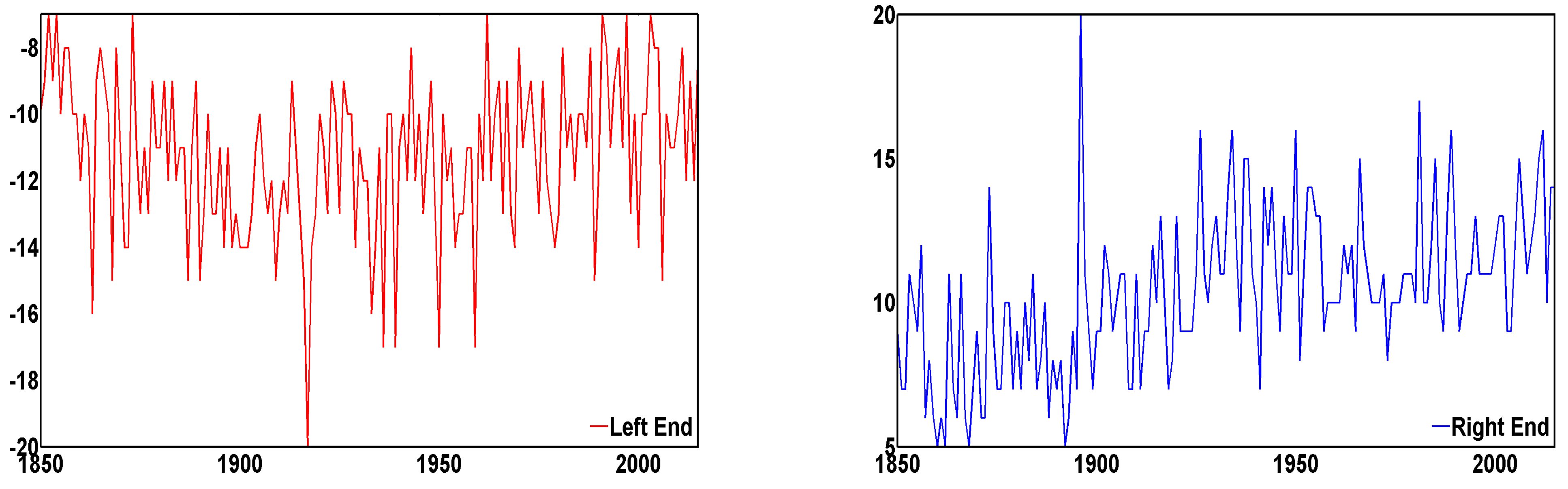
Further, 99 percent of the total probability mass is exploited as the support of the temperature anomaly distribution at each time t because 0.5 percent of the probability mass at each end would be an adequate threshold to minimize the estimation errors induced by the boundary problem from the standard kernel density estimation technique. Figure 1 shows the time series of left and right ends of the chosen support of the global temperature anomaly distribution, indicating that non-common support would be necessary to effectively generate the distributions of temperature anomaly. Specifically, the right end of the support of the global temperature anomaly distribution reveals an increasing trend, implying the warming phenomena.
For the radiative forcing variable, TRF data from 1850 to 2015 (Hansen et al. 2017) are employed, which represent the sum of anthropogenic forcing and natural variability. Specifically, TRF is the sum of well-mixed GHG (CO 2 , CH 4 , N 2 O, and CFCs), ozone, surface albedo and tropospheric aerosols, and solar irradiance.
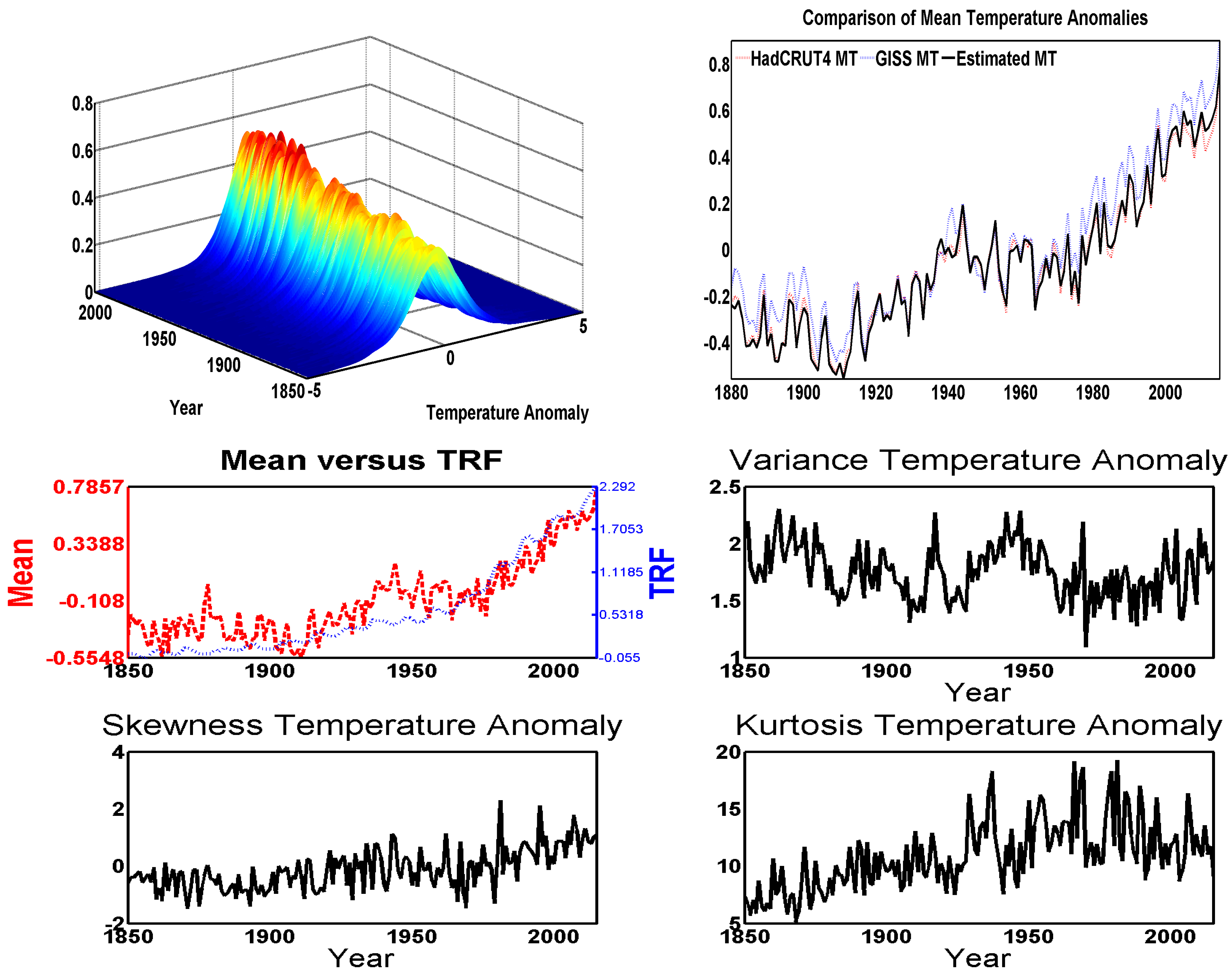
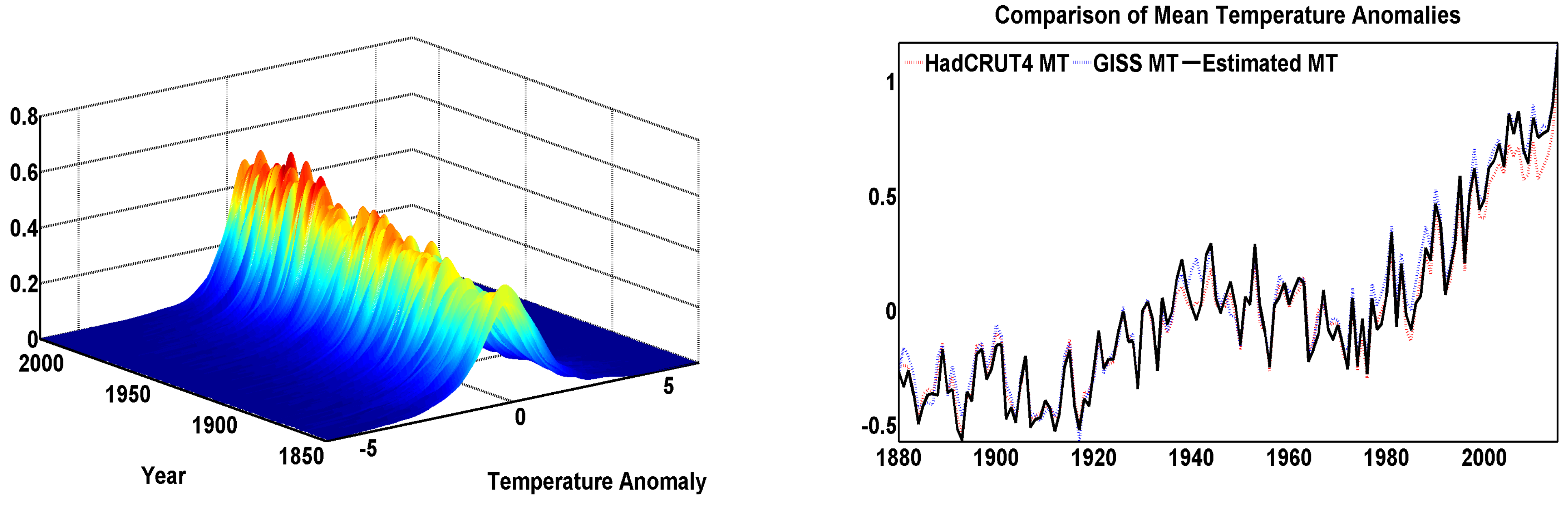
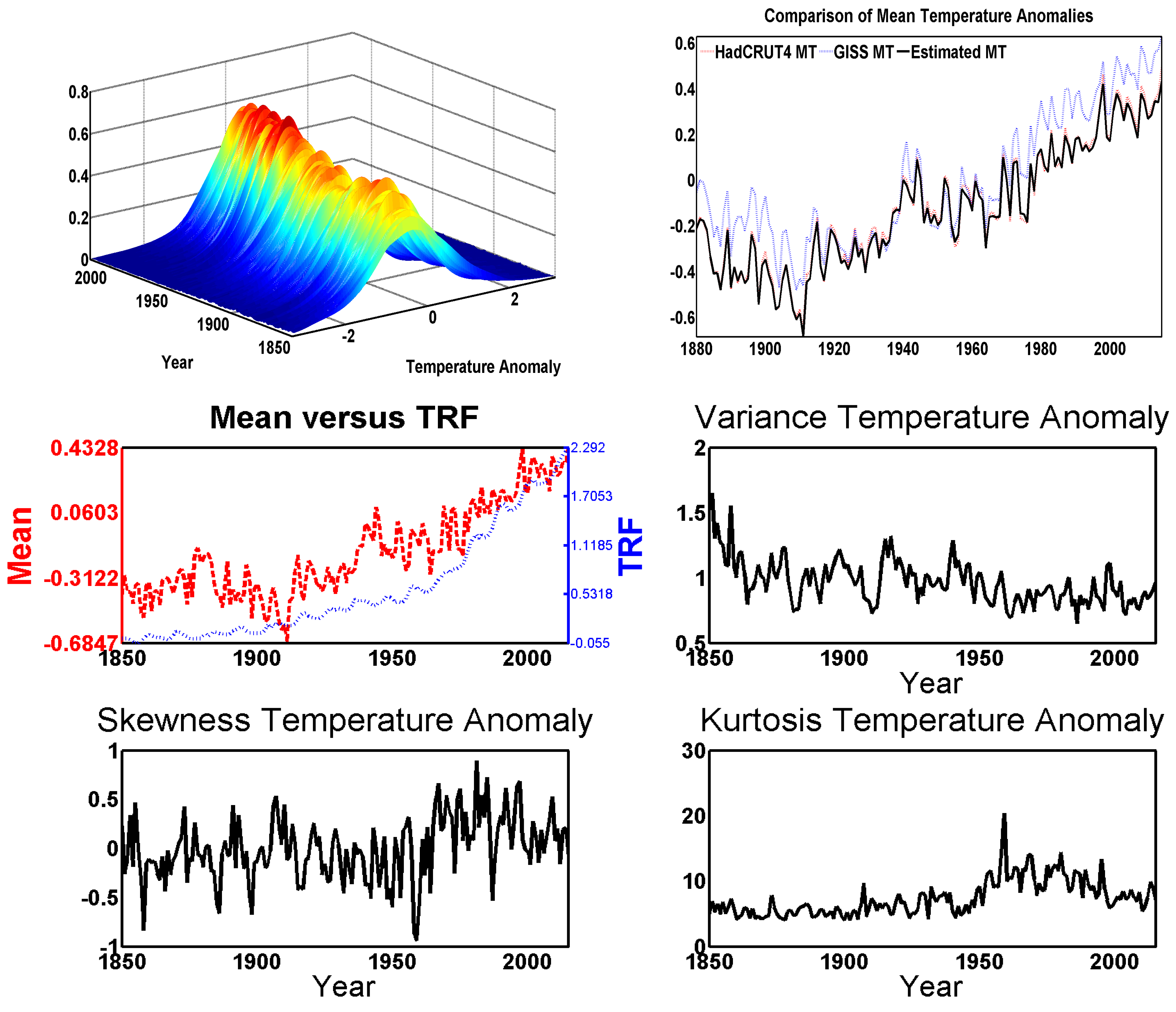
10 Figure 2, Figure 3 and Figure 4 provide detailed information of the temperature anomaly distribution for the Globe, Northern Hemisphere, and Southern Hemisphere and TRF. Specifically, the top-left panels of Figure 2, Figure 3 and Figure 4 show the temperature anomaly distribution generated by the procedure of Chang et al. (2020), and the top-right panels of the figures illustrate the graphical comparison between the first moment estimated from the generated temperature anomaly distribution and the web-posted mean temperature anomalies from the GISS11 and HadCRUT4 (the median of the 100 ensemble member time series)12 websites for the Globe, Northern Hemisphere, and Southern Hemisphere.
Indeed, 99 percent of probability mass in estimating the temperature anomaly distribution provides a good approximation for estimating the first moment (i.e., mean temperature anomaly) at each time t, in the sense that estimated mean temperature anomalies are similar to mean temperature anomalies widely-used by climate scientists. Note that the GISS surface temperature data are expressed as an anomaly in degrees Celsius with the base period 1951–1980, which is available after the year 1880. As mentioned earlier, the differences in the mean temperature anomalies between the HadCRUT4 and GISS sources are greater for the Southern Hemisphere, in which the GISS team interpolates the sea-surface temperature data.
The bottom panels of Figure 2, Figure 3 and Figure 4 provide the first four central moments of the generated temperature anomaly distribution. While the variances of the estimated temperature anomaly distribution have decreased, roughly similar to Chang et al. (2020), the means, the skewness, and the kurtosis of the estimated temperature anomaly distribution have increased. In particular, the skewness appears to have increased from negative to positive. These statistical facts imply that the temperature anomaly distributions have been concentrated around their increasing means, and the probabilities of extremely positive temperature anomalies have increased. Not surprisingly, the decreasing variances of the temperature anomaly distribution would be on the same lines with the movements of the other central moments. Lastly, the calculated mean temperature anomalies are compared with the TRF variable, clearly showing that they moved together for the last 165 years.

5. Empirical Analysis

Throughout this study, the statistical testing result of the unit-root type nonstationarity of Chang et al. (2020) was followed. Specifically, the estimated persistence of the global mean temperature anomaly was closer to a stochastic trend, but not high enough to a deterministic trend, implying that no linear deterministic trend has been detected. As some econometricians discover a broken deterministic trend from the global mean temperature anomaly (Gay-Garcia et al. 2009; Estrada et al. 2013b, inter alia), moreover, Gao and Hawthorne (2006) attempt to estimate a general deterministic trend by allowing the flexible nonlinearity in the deterministic trend component. However, Chang et al. (2020) argue that a deterministic trend with the excessive nonlinearity and variability could be better expressed as a stochastic trend. Subsequently, the failure of rejection of the cointegration test implies that the TRF variable shares a stochastic trend with the global temperature anomaly distribution.
In the literature, climate sensitivity for the Globe is estimated as the value 0.43 ° C/(W/m 2 ) and 0.35 ° C/(W/m 2 ) with AMO-unfiltered HadCRUT4 and NASA dataset, respectively (Estrada et al. 2013b).13 As expected, linear climate sensitivity is estimated as the value 0.435 ° C/(W/m 2 ), which is a similar value to the Global case.
Table 1 provides the estimation result of Equation (13) with a derivative of interest. Based on AIC and BIC criteria, the optimal models for the Globe, Northern Hemisphere, and Southern Hemisphere are ( p = 2 , q = 1 ) , ( p = 2 , q = 1 ) , and ( p = 2 , q = 0 ) , respectively. Moreover, the first VAT test statistics (VAT 1 ) for the Globe, Northern Hemisphere, and Southern Hemisphere cases as well as for linear/optimally chosen nonlinear models, indicate that all considered models are authentic, supporting the cointegration technique using the CCR methodology. However, the second VAT test statistics (VAT 2 ) indicate that all regression models could be spurious if we assume the strict stationarity in the residual. Notice that the second VAT statistics decreased by considering the nonlinear temperature term for the Globe and Northern Hemisphere cases, indicating that the nonlinear temperature term s t 2 in Equation (18) plays a role in explaining the oceanic multidecadal oscillation.
The nonlinear estimator D 1 represents climate sensitivity that considers all nonlinear effects across the observed temperature anomalies. The resulting climate sensitivity, D 1 , of the nonlinear cointegration model is provided as the value 0.380 for the Globe, indicating that the global mean temperature anomaly increases by 0.380 ° C when TRF increases by 1 W/m 2 . In the meantime, the misspecification error of the linear model is greatest for the Northern Hemisphere (0.1077 ° C/(W/m 2 )), and lowest for the Southern Hemisphere (0.0402 ° C/(W/m 2 )). The Wald test decisively rejects the null of no statistical significance of the nonlinear temperature term for the Globe, Northern Hemisphere, and Southern Hemisphere cases (p-values are less than 0.01).
As shown by Figure 2, Figure 3 and Figure 4, TRF has affected not only the mean temperature anomaly, but also variance, skewness, and kurtosis temperature anomalies for approximately 150 years. This implies that the Earth’s surface temperature has been affected by human and natural forcing in a spatially heterogenous manner. The nonlinear cointegration model enables us to estimate the true effect by including the spatial distributions of temperature anomalies in the model, showing that the change in the global mean temperature anomaly associated with TRF (0.380 ° C/(W/m 2 )) would be less than what we have observed (0.435 ° C/(W/m 2 )).
In the literature, the transient climate response is often calculated as the global mean temperature response in ° C to a doubling of atmospheric CO 2 from pre-industrial level by an increase of 1 percent per year. Schwartz (2012) estimates the value 3.71 W/m 2 of the TRF level at the time when the atmospheric CO 2 is doubled from the pre-industrial level. Subsequently, the transient climate response is calculated as the value 1.410 ° C (=3.71 × 0.380 ° C/(W/m 2 )), which is 0.204 ° C lower than the estimated transient climate response from the linear model (1.614 ° C). Given that the global mean temperature anomaly was 0 . 40 ° C in 1850, the predicted global mean temperature anomaly associated with a doubled atmospheric CO 2 level is 1.01 ° C.
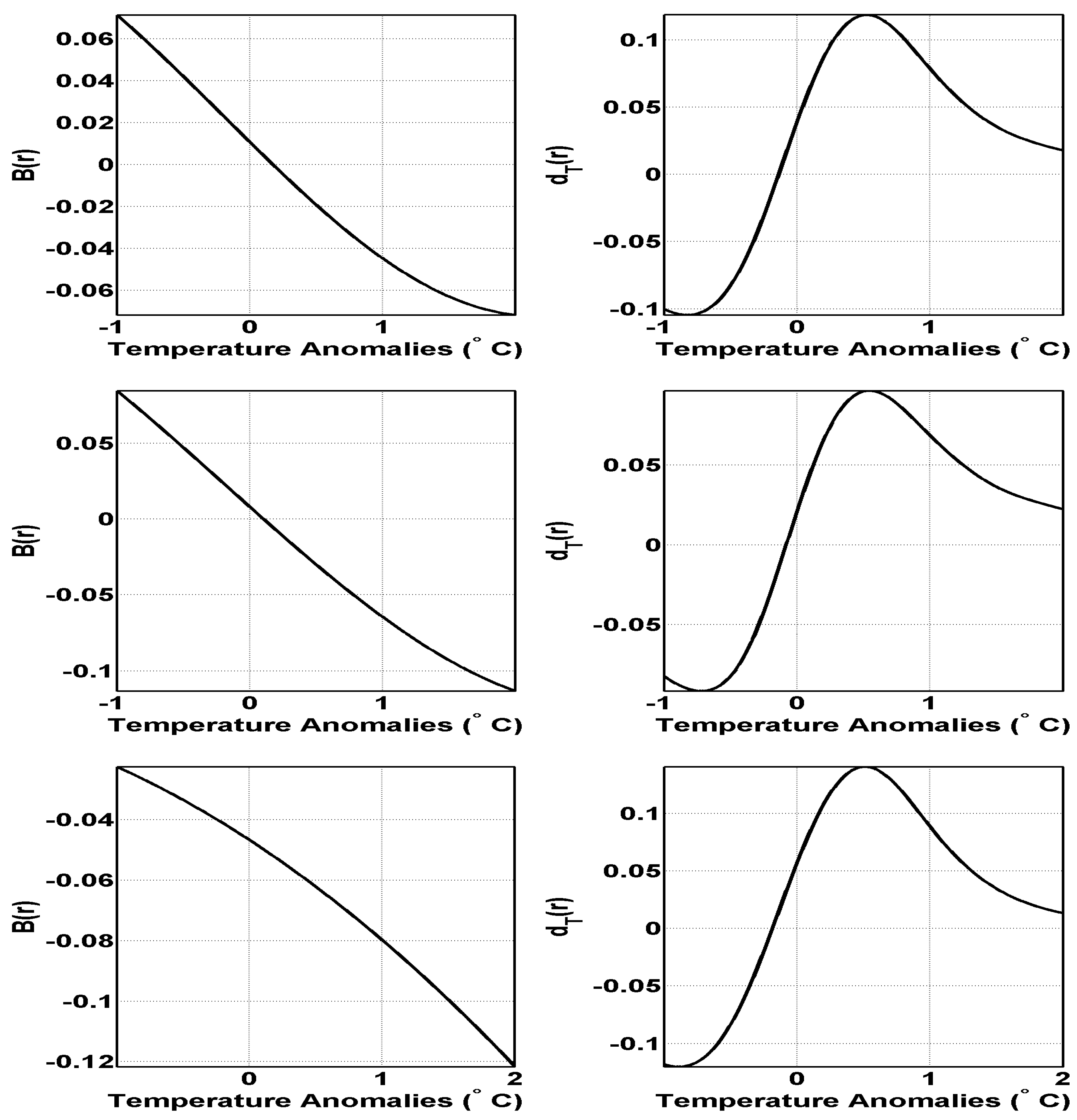
Climatologically, the TRF response function at temperature anomaly r 0 , D 2 ( r 0 ) , indicates a change in the mean temperature anomaly, if net incoming absorbed radiation is solely determined by temperature anomaly r 0 . As such, the nonlinear effect, in addition to the mean effect (or linear effect), would provide the temperature-dependent TRF effect on the mean temperature anomaly. The nonlinear effects of the estimated climate sensitivity, D ^ 1 , are calculated as values −0.018 ° C/(W/m 2 ), −0.025 ° C/(W/m 2 ), and −0.009 ° C/(W/m 2 ) for the Globe, Northern Hemisphere, and Southern Hemisphere (i.e., the term, D r B ( r ) f t ( r ) d r / h t in Equation (10)). Therefore, we may conclude that the nonlinearity of the relationship induced by the spatial heterogeneity was strongest for the Northern Hemisphere.
In Figure 5, both the net incoming absorbed radiation, B ( r ) , and the derivative of the temperature anomaly distribution with respect to TRF, d T ( r ) , are presented for the Globe, Northern Hemisphere, and Southern Hemisphere. Note that the domain of the temperature anomaly is shortened below −1.0 ° C and above 2.0 ° C for a practical purpose. The left panels of Figure 5 illustrate that the nonlinear effect becomes more significant in the opposite direction as the temperature anomaly approaches the left and right ends. As mentioned in Section 3, more specifically, B ( r ) estimates the effect of net incoming absorbed radiation of the regions that are represented by the temperature anomaly r.
Note that the popular term, “polar amplification,” states that the low (high) temperature anomaly region, which mainly represents higher (lower) latitude areas, is related to the mean temperature anomaly in a positive (negative) direction (Boer and Yu 2003). Consistent with this notion, a positive (negative) value of the net incoming absorbed radiation term, B ( r ) implies that the TRF effect under linearity would be underestimated (overestimated). In other words, the TRF effect under linearity should be amplified for the negative anomalies (high latitude areas) for the Globe and Northern Hemisphere, and be attenuated for the positive anomalies (low latitude areas) for the Globe, Northern Hemisphere, and Southern Hemisphere.
By considering the nonlinear temperature term with the derivative of the temperature anomaly distribution with respect to TRF, B ( r ) d T ( r ) , the nonlinear TRF effect would be obtained by amplifying or attenuating the linear TRF effect (see Equation (11)). Since the changes in probability with respect to the change in TRF (i.e., d T ( r ) ) are very small at extreme temperature anomalies, the nonlinear effects at extreme temperature anomalies could be much less than those at low or high temperature anomalies.
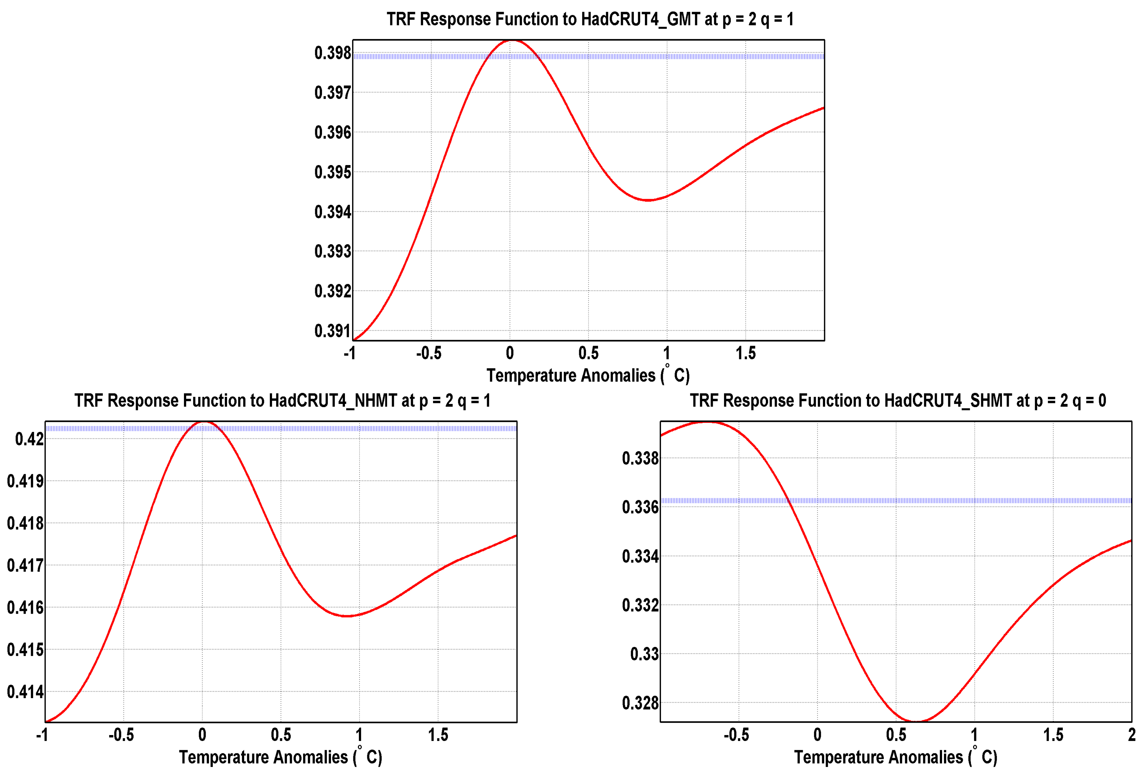
Figure 6 illustrates the TRF response function for the Globe, Northern Hemisphere, and Southern Hemisphere, which is the estimator D 2 ( r ) for r D r in Equation (11). The reference (dashed blue) line represents the linear TRF response function, postulating that the TRF effect on the mean temperature anomaly is constant across temperature anomalies. That is, it illustrates the TRF effect on the mean temperature anomaly without the nonlinear effect. For the Globe, the linear term provides an estimate of the constant climate sensitivity as the value 0.40 ° C/(W/m 2 ), and the nonlinear TRF response function intersects with the linear TRF response function at two anomalies, −0.14 ° C and 0.18 ° C. This implies that the linear TRF response function underestimates the true effect between these two anomalies.
In Figure 6, more importantly, the nonlinear TRF response function (i.e., nonlinear climate sensitivity) provides an interpretation of the relative magnitude of the TRF effect on the mean temperature anomaly. In particular, the greatest temperature-dependent TRF effect on the global mean temperature anomaly is estimated as the value 0.398 ° C/(W/m 2 ), if net incoming absorbed radiation is solely determined by a temperature anomaly, 0.015 ° C. That is, the spatial contribution to the change in the global mean temperature anomaly is strongest for the areas in which their temperature levels correspond to 0.015 ° C. Such spatially heterogeneous contributions could be better understood by incorporating the higher-order moments of spatial distributions of temperature anomaly in the nonlinear cointegration model.
Moreover, the smoothed global mean temperature anomaly using a polynomial function was approximately 0.01 ° C in 1974, implying that the TRF effect on the global mean temperature anomaly would be strongest in 1974. Note that the sum of nonlinear effects of estimator D 2 ( r ) across temperature anomaly in Equation (11) is equal to the nonlinear effect of estimator D 1 in Equation (10). In this light, the high degrees of nonlinearity could be estimated by adding all nonlinear effects, although the magnitude of nonlinear effect at each temperature anomaly is small. Further note that the nonlinear TRF effect for the Northern Hemisphere case shows a similar pattern to the Global case. However, its effect is greater than the Global case because the speed of global warming is faster in the Northern Hemisphere than in the Southern Hemisphere.
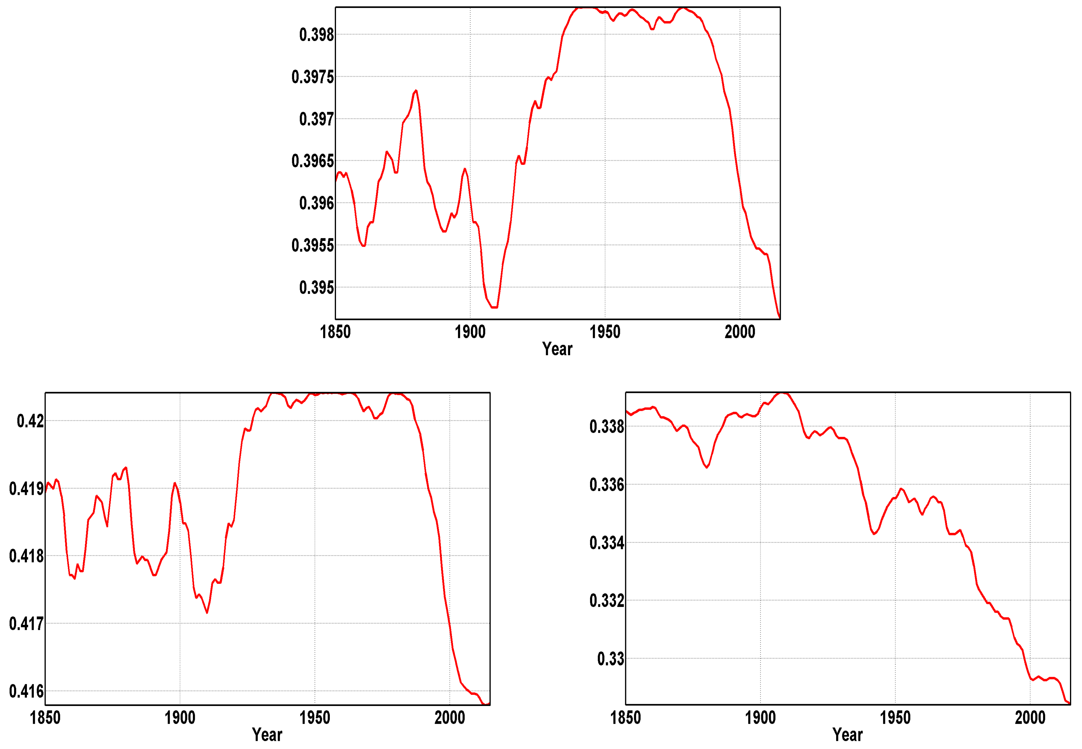
To elaborate on this discussion, Figure 7 provides the nonlinear TRF response function over time. Specifically, I postulate that the spatial regions where provide the biggest contribution on the change of mean temperature anomaly at time t is located at the areas where have a record of the mean temperature anomaly at time t. This is a reasonable situation, in the sense that the mean value of spatial distribution would be largely determined by the spatial areas where have a similar or closer mean value. Consequently, the value of the nonlinear TRF response function at time t indicates the relative magnitude of the TRF effect when the biggest spatial contribution is evaluated at the mean temperature anomaly at time t.14
The TRF response functions presented in Figure 7 imply that the warming speed of the Globe and Northern Hemisphere has decreased since 1980. However, the speed would start to increase when the mean temperature anomaly reaches approximately 0.8 ° C. Notably, the presented TRF response function for the Southern Hemisphere has decreased since 1910. Similar to the Globe and Northern Hemisphere cases, however, the warming speed of the Southern Hemisphere would start to increase when the mean temperature anomaly reaches approximately 0.7 ° C, which is much earlier compared to other cases. Based on the information provided by the HadCRUT4 website,15 the mean temperature anomalies for the Globe, Northern Hemisphere, and Southern Hemisphere in 2019 were estimated at 0.736 ° C, 0.972 ° C, and 0.502 ° C, respectively, indicating that the warming speed of the Northern Hemisphere has already started to increase.

6. Conclusions

In this paper, I proposed the nonlinear cointegration model based on the well-known EBCM. For this, the nonlinear cointegrating regression of the mean temperature anomaly for the Globe, Northern Hemisphere, and Southern Hemisphere, were estimated using the spatial distributions of temperature anomalies. Subsequently, the nonlinear TRF effect on the mean temperature anomaly was estimated, suggesting that the TRF effect on the mean temperature anomaly would be temperature-dependent for the Globe, Northern Hemisphere, and Southern Hemisphere. Graphically, the TRF response function has a flexible shape to represent the change in the mean temperature anomaly when net incoming absorbed radiation is hypothetically determined at some temperature anomaly.
Statistically, the linear model fails to take into account the net incoming absorbed radiation term, which would cause the slope estimator to be invalid. Considering the functional form of net incoming absorbed radiation, the proposed nonlinear cointegration model shows the reasonable nonlinear dependence structure between the mean temperature anomaly and TRF. Specifically, climate sensitivity is estimated to be temperature-dependent (or spatially heterogenous), providing that the estimated nonlinear climate sensitivity was highest in the mid-1970s for the Globe. Moreover, the TRF effect on the mean temperature anomaly, which considers all nonlinear effects, is less than the estimate of the linear climate sensitivity provided by the literature. Lastly, the statistical testing results indicate that the linear model possesses a significant misspecification error for the Globe, Northern Hemisphere, and Southern Hemisphere cases.
The next step regarding this research refers to climate variability. As emphasized by Brock et al. (2013), spatial complexity on Earth is a big challenge for analyzing temperature series at hemispheric scales. The complexity inherited from spatial diversity produces hardly explainable natural variability through the observed data. At least to date, the well-known inter-annual global variability or hemispheric climate variability is regarded as the El Niño/Southern Oscillation (ENSO), the North Atlantic Oscillation (NAO), and the Atlantic Multidecadal Oscillation (AMO). Among them, the most influential natural variation for the attribution study is the AMO, which could distort the long-term global warming trend. Specifically, the large ocean-atmosphere cycle over the North Atlantic, which is defined as approximately 60 to 90 years of low-frequency patterns of sea surface temperature variability, explains the larger variability in Northern Hemisphere temperatures and therefore, globally.
In particular, Estrada et al. (2013b) identified its difficulty when they conducted an attribution study. They argued that the detrended Global and Northern Hemisphere temperatures with forcing variables could be further explained by the AMO and therefore the difference between the dates of a structural break could be explained as well. In light of this, Estrada et al. (2013b) filtered the AMO information from the Global and Northern Hemisphere mean temperature anomalies to estimate constant climate sensitivity. To put these factors into perspective, it is worth estimating nonlinear climate sensitivity after extracting the major climate variabilities.
Moreover, the uncertainty of the estimator of the TRF response function needs to be evaluated. As the estimation is implemented via two-step approach, it is difficult to evaluate the bootstrapping confidence bands, in the sense that the estimator’s uncertainty comes from both steps. We may estimate the uncertainty by fixing the point estimate of the first step as a constant. Since the first step is the nonstationary nonlinear regression model, however, the uncertainty of the first step’s estimator would be larger than that of the second step’s estimator. I leave these tasks to future research.

Funding

This research received no external funding.

Data Availability Statement

The data presented in this study are available on request from the corresponding author. The data are not publicly available due to privacy.

Acknowledgments

The authors deeply appreciate all valuable comments from Zack Miller, David M. Kaplan, Shawn Ni, Yeji Lim, and Sanha Noh and to participants of a Brown bag seminar at the MU Department of Economics, the Missouri Valley Economic Association (MVEA) conference (St. Louis, 2016), and the 2020 virtual summer meeting of Korean Resource Economics Association for useful feedback.

Conflicts of Interest

The author declares no conflict of interest.

References

  1. Bierens, Herman J. 2000. Nonparametric nonlinear cotrending analysis, with an application to interest and inflation in the united states. Journal of Business & Economic Statistics 18: 323–37. [Google Scholar]
  2. Bindoff, Nathaniel L., Peter A. Stott, Krishna Mirle AchutaRao, Myles R. Allen, Nathan Gillett, David Gutzler, Kabumbwe Hansingo, G. Hegerl, Yongyun Hu, Suman Jain, and et al. 2013. Detection and attribution of climate change: From global to regional. In The Physical Science Basis, Contribution of Working Group I to the Fifth Assessment Report of the Intergovernmental Panel on Climate Change. Cambridge: Cambridge University Press, pp. 867–952. [Google Scholar]
  3. Boer, George, and Bin Yu. 2003. Climate sensitivity and response. Climate Dynamics 20: 415–29. [Google Scholar] [CrossRef]
  4. Brock, William A., Gustav Engström, Dieter Grass, and Anastasios Xepapadeas. 2013. Energy balance climate models and general equilibrium optimal mitigation policies. Journal of Economic Dynamics and Control 37: 2371–96. [Google Scholar] [CrossRef]
  5. Budyko, Mikhail I. 1969. The effect of solar radiation variations on the climate of the earth. Tellus 21: 611–19. [Google Scholar] [CrossRef] [Green Version]
  6. Campbell, Sean D., and Francis X. Diebold. 2005. Weather forecasting for weather derivatives. Journal of the American Statistical Association 100: 6–16. [Google Scholar] [CrossRef] [Green Version]
  7. Chang, Yoosoon, Chang Sik Kim, J. Isaac Miller, Joon Y. Park, and Sungkeun Park. 2014. Time-varying long-run income and output elasticities of electricity demand with an application to korea. Energy Economics 46: 334–47. [Google Scholar] [CrossRef]
  8. Chang, Yoosoon, Chang Sik Kim, J. Isaac Miller, Joon Y. Park, and Sungkeun Park. 2016a. A new approach to modeling the effects of temperature fluctuations on monthly electricity demand. Energy Economics 60: 206–16. [Google Scholar] [CrossRef] [Green Version]
  9. Chang, Yoosoon, Chang Sik Kim, and Joon Y. Park. 2016b. Nonstationarity in time series of state densities. Journal of Econometrics 192: 152–67. [Google Scholar] [CrossRef] [Green Version]
  10. Chang, Yoosoon, Robert K Kaufmann, Chang Sik Kim, J. Isaac Miller, Joon Y. Park, and Sungkeun Park. 2020. Evaluating trends in time series of distributions: A spatial fingerprint of human effects on climate. Journal of Econometrics 214: 274–94. [Google Scholar] [CrossRef]
  11. Estrada, Francisco, and Pierre Perron. 2014. Detection and attribution of climate change through econometric methods. Boletín de la Sociedad Matemática Mexicana 20: 107–36. [Google Scholar] [CrossRef]
  12. Estrada, Francisco, Pierre Perron, Carlos Gay-García, and Benjamín Martínez-López. 2013a. A time-series analysis of the 20th century climate simulations produced for the ipcc’s fourth assessment report. PLoS ONE 8: e60017. [Google Scholar] [CrossRef] [Green Version]
  13. Estrada, Francisco, Pierre Perron, and Benjamín Martínez-López. 2013b. Statistically derived contributions of diverse human influences to twentieth-century temperature changes. Nature Geoscience 6: 1050–55. [Google Scholar] [CrossRef] [Green Version]
  14. Fasullo, John T., and Kevin E. Trenberth. 2012. A less cloudy future: The role of subtropical subsidence in climate sensitivity. Science 338: 792–94. [Google Scholar] [CrossRef] [PubMed]
  15. Gallant, A. Ronald. 1981. On the bias in flexible functional forms and an essentially unbiased form: The fourier flexible form. Journal of Econometrics 15: 211–45. [Google Scholar] [CrossRef]
  16. Gao, Jiti, and Kim Hawthorne. 2006. Semiparametric estimation and testing of the trend of temperature series. The Econometrics Journal 9: 332–55. [Google Scholar] [CrossRef]
  17. Gay-Garcia, Carlos, Francisco Estrada, and Armando Sánchez. 2009. Global and hemispheric temperatures revisited. Climatic Change 94: 333–49. [Google Scholar] [CrossRef]
  18. Hansen, James E., and Makiko Sato. 2012. Paleoclimate implications for human-made climate change. In Climate Change. Edited by A. Berger, F. Mesinger and D. Sijacki. Vienna: Springer, pp. 21–47. [Google Scholar]
  19. Hansen, James, Makiko Sato, Pushker Kharecha, and Karina von Schuckmann. 2011. Earth’s energy imbalance and implications. Atmospheric Chemistry and Physics 11: 13421–49. [Google Scholar] [CrossRef] [Green Version]
  20. Hansen, James, Makiko Sato, Gary Russell, and Pushker Kharecha. 2013. Climate sensitivity, sea level and atmospheric carbon dioxide. Philosophical Transactions of the Royal Society A: Mathematical, Physical and Engineering Sciences 371: 20120294. [Google Scholar] [CrossRef]
  21. Hansen, James, Makiko Sato, Pushker Kharecha, Karina von Schuckmann, David J. Beerling, Junji Cao, Shaun Marcott, Valerie Masson-Delmotte, Michael J. Prather, Eelco J. Rohling, and et al. 2017. Young people’s burden: Requirement of negative CO2 emissions. Earth System Dynamics 8: 577–616. [Google Scholar] [CrossRef] [Green Version]
  22. Held, Isaac M., and Max J. Suarez. 1974. Simple albedo feedback models of the icecaps. Tellus 26: 613–29. [Google Scholar] [CrossRef]
  23. IPCC. 2007. Summary for Policymakers Climate Change 2007: The Physical Science Basis. Contribution of Working Group I to the Fourth Assessment Report of the Intergovernmental Panel on Climate Change. Edited by S. Solomon, D. Qin, M. Manning, Z. Chen, M. Marquis, K. B. Averyt, M. Tignor and H. L. Miller. Cambridge and New York: Cambridge University Press. [Google Scholar]
  24. IPCC. 2014. Climate Change 2014: Mitigation of Climate Change. Contribution of Working Group III to the Fifth Assessment Report of the Intergovernmental Panel on Climate Change. Edited by O. Edenhofer, R. Pichs-Madruga, Y. Sokona, E. Farahani, S. Kadner, K. Seyboth, A. Adler, I. Baum, S. Brunner, P. Eickemeier and et al. Cambridge and New York: Cambridge University Press. [Google Scholar]
  25. Kaufmann, Robert K., and David I. Stern. 2002. Cointegration analysis of hemispheric temperature relations. Journal of Geophysical Research: Atmospheres 107: ACL-8. [Google Scholar] [CrossRef] [Green Version]
  26. Kaufmann, Robert K., Heikki Kauppi, and James H. Stock. 2006a. Emissions, concentrations & temperature: A time series analysis. Climatic Change 77: 249–78. [Google Scholar]
  27. Kaufmann, Robert K., Heikki Kauppi, and James H. Stock. 2006b. The relationship between radiative forcing and temperature: What do statistical analyses of the instrumental temperature record measure? Climatic Change 77: 279–89. [Google Scholar] [CrossRef] [Green Version]
  28. Kaufmann, Robert K., Heikki Kauppi, and James H. Stock. 2010. Does temperature contain a stochastic trend? Evaluating conflicting statistical results. Climatic Change 101: 395–405. [Google Scholar] [CrossRef]
  29. Kaufmann, Robert K., Heikki Kauppi, Michael L. Mann, and James H. Stock. 2013. Does temperature contain a stochastic trend: Linking statistical results to physical mechanisms. Climatic Change 118: 729–43. [Google Scholar] [CrossRef]
  30. Knutti, Reto, Maria A. A. Rugenstein, and Gabriele C. Hegerl. 2017. Beyond equilibrium climate sensitivity. Nature Geoscience 10: 727–36. [Google Scholar] [CrossRef]
  31. Loeb, Norman G., John M. Lyman, Gregory C. Johnson, Richard P. Allan, David R. Doelling, Takmeng Wong, Brian J. Soden, and Graeme L. Stephens. 2012. Observed changes in top-of-the-atmosphere radiation and upper-ocean heating consistent within uncertainty. Nature Geoscience 5: 110–13. [Google Scholar] [CrossRef]
  32. Miller, J. Isaac. 2017. Local Climate Sensitivity: A Statistical Approach for a Spatially Heterogeneous Planet. Working Paper. Columbia: University of Missouri, Department of Economics. [Google Scholar]
  33. Miller, J. Isaac, and Kyungsik Nam. 2020. Dating hiatuses: A statistical model of the recent slowdown in global warming and the next one. Earth System Dynamics 11: 1123–32. [Google Scholar] [CrossRef]
  34. Morana, Claudio, and Giacomo Sbrana. 2019. Climate change implications for the catastrophe bonds market: An empirical analysis. Economic Modelling 81: 274–94. [Google Scholar] [CrossRef]
  35. Morice, Colin P., John J. Kennedy, Nick A. Rayner, and Phil D. Jones. 2012. Quantifying uncertainties in global and regional temperature change using an ensemble of observational estimates: The hadcrut4 data set. Journal of Geophysical Research: Atmospheres 117: D8. [Google Scholar] [CrossRef]
  36. Newey, Whitney K., and Kenneth D. West. 1994. Automatic lag selection in covariance matrix estimation. The Review of Economic Studies 61: 631–53. [Google Scholar] [CrossRef]
  37. North, Gerald R., John G. Mengel, and David A. Short. 1983. Simple energy balance model resolving the seasons and the continents: Application to the astronomical theory of the ice ages. Journal of Geophysical Research: Oceans 88: 6576–86. [Google Scholar] [CrossRef]
  38. Park, Joon Y. 1990. Testing for unit roots and cointegration by variable addition. Advances in Econometrics 8: 107–33. [Google Scholar]
  39. Park, Joon Y. 1992. Canonical cointegrating regressions. Econometrica 60: 119–43. [Google Scholar] [CrossRef]
  40. Park, Joon Y., Kwanho Shin, and Yoon-Jae Whang. 2010. A semiparametric cointegrating regression: Investigating the effects of age distributions on consumption and saving. Journal of Econometrics 157: 165–78. [Google Scholar] [CrossRef]
  41. Perron, Pierre, and Francisco Estrada. 2012. Breaks, Trends and the Attribution of Climate Change: A Time-Series Analysis. Technical Report. Boston: Department of Economics, Boston University. [Google Scholar]
  42. Petit, Jean-Robert, Jean Jouzel, Dominique Raynaud, Narcisse I. Barkov, J.-M. Barnola, Isabelle Basile, and Michael Bender. 2001. Climate and atmospheric history of the past 420,000 years from the Vostok ice core, Antarctica. Nature 399: 429–36. [Google Scholar] [CrossRef] [Green Version]
  43. Pretis, Felix. 2020. Econometric modelling of climate systems: The equivalence of energy balance models and cointegrated vector autoregressions. Journal of Econometrics 214: 256–73. [Google Scholar] [CrossRef]
  44. Schwartz, Stephen E. 2012. Determination of earth’s transient and equilibrium climate sensitivities from observations over the twentieth century: Strong dependence on assumed forcing. Surveys in Geophysics 33: 745–77. [Google Scholar] [CrossRef]
  45. Stern, Nicholas. 2008. The economics of climate change. American Economic Review 98: 1–37. [Google Scholar] [CrossRef] [Green Version]
1.
For HadCRUT4 dataset, the zero-base period is from 1961M1 to 1990M12.
2.
Outgoing radiation is set as a linear function of the Earth’s surface temperature and cloudiness (Budyko 1969; Fasullo and Trenberth 2012). Due to complexity and data uncertainty of the cloud dynamics, however, I presume the simplest function for outgoing radiation (i.e., I r ^ , t = O r ^ s r ^ , t as in Brock et al. 2013).
3.
I acknowledge that the constant heat capacity is an excessively restrictive assumption. Since the goal of this study is to develop the statistical model based on underlying physics while the non-constant heat capacity makes the model too complicated, I assume a phenomenological constant heat capacity (Brock et al. 2013). However, this issue is addressed in another working paper (see Miller and Nam 2020).
4.
Note that scientific literature uses the atmospheric CO 2 concentration as external forcing instead of TRF. Contrastingly, I consider TRF because the purpose of this study is to build a statistical model, so it is important to include all external forcing in the regression model that could affect the global climate system.
5.
This study focuses on developing a reduced-form nonlinear cointegrating regression model based on the EBCM. However, Miller (2017) provides the climatological modeling with the first law of thermodynamics (i.e., integrating net incoming absorbed radiation across the globe is zero, but with non-zero derivatives).
6.
Note that s r ^ , t in the Global EBCM (2) is the observed temperature anomaly at location r ^ and time t, and r t in reduced form Equation (7) is the temperature anomaly observed on the surface of the Earth. Therefore, they are regarded as the same variable.
7.
The estimates of Miller and Nam (2020) show that the Oceanic Multidecadal Oscillation has 76 year period, 3 year phase shift, and 0.130 amplitude.
8.
Ensemble median of HadCRUT4.6.0.0 downloaded from http://www.metoffice.gov.uk/hadobs/hadcrut4/data/current/download.html on 29 December 2019.
9.
10.
Downloaded from www.columbia.edu/~mhs119/Burden on 30 January 2018.
11.
http://data.giss.nasa.gov/gistemp/, assessed on 29 December 2019.
12.
http://www.metoffice.gov.uk/hadobs/hadcrut4/, assessed on 29 December 2019.
13.
With the AMO-filtered HadCRUT4 (version 4.2.0.0) and NASA dataset, climate sensitivity is estimated by 0.40 ° C/(W/m 2 ) and 0.39 ° C/(W/m 2 ), respectively.
14.
The four-year moving average mean temperature anomaly is applied to calculate the TRF response function over time, in order to exclude the ENSO-induced short-run variability in the discussion.
15.
Figure 1. Time–series of left and right ends of the support of the global temperature anomaly distribution.
Econometrics 09 00006 g001
Figure 2. Global temperature anomaly densities and moments.
Econometrics 09 00006 g002
Figure 3. Northern hemisphere temperature anomaly densities and moments.
Econometrics 09 00006 g003aEconometrics 09 00006 g003b
Figure 4. Southern hemisphere temperature anomaly densities and moments.
Econometrics 09 00006 g004
Figure 5. Nonlinear response function B ( r ) and d T ( r ) for Globe (top)/NH (middle)/SH (bottom).
Econometrics 09 00006 g005
Figure 6. Nonlinear TRF response function over temperature anomaly for Globe (top)/NH (left bottom)/SH (right bottom) (see Equation (11)).
Econometrics 09 00006 g006
Figure 7. Nonlinear TRF response function over year for Globe (top)/NH (left bottom)/SH (right bottom).
Econometrics 09 00006 g007
Table 1. Estimation results.
Global Temperature Anomaly
pq D 1 Error(r) b 1 CCR T-StatAICBIC VAT 1 Stat VAT 2 StatWALD Stat
100.4350.0000.43520.191−217.336−211.1121.30342.6140.000
210.3800.0550.39818.085−244.910−229.3502.99822.73722.962
Northern Hemisphere Temperature Anomaly
pq D 1 Error(r) b 1 CCR T-StatAICBIC VAT 1 Stat VAT 2 StatWALD Stat
100.5030.0000.50316.427−95.034−88.8101.22953.3970.000
210.3950.1080.42013.289−125.168−109.6080.08121.76028.836
Southern Hemisphere Temperature Anomaly
pq D 1 Error(r) b 1 CCR T-StatAICBIC VAT 1 Stat VAT 2 StatWALD Stat
100.3670.0000.36719.058−256.415−250.1913.8468.2140.000
200.3270.0400.33615.553−268.311−258.9750.59212.0407.708
Publisher’s Note: MDPI stays neutral with regard to jurisdictional claims in published maps and institutional affiliations.

