On the Asymptotic Distribution of Ridge Regression Estimators Using Training and Test Samples

Abstract

The asymptotic distribution of the linear instrumental variables (IV) estimator with empirically selected ridge regression penalty is characterized. The regularization tuning parameter is selected by splitting the observed data into training and test samples and becomes an estimated parameter that jointly converges with the parameters of interest. The asymptotic distribution is a nonstandard mixture distribution. Monte Carlo simulations show the asymptotic distribution captures the characteristics of the sampling distributions and when this ridge estimator performs better than two-stage least squares. An empirical application on returns to education data is presented.

1. Introduction

This paper concerns the estimation and inference on the structural parameters in the linear instrumental variables (IV) model estimated with ridge regression. This estimator differs from previous ridge regression estimators in three important areas. First, the regularization tuning parameter is selected using a randomly selected test sample from the observed data. Second, the empirically selected tuning parameter’s impact on the estimates of the parameters of interest is accounted for by deriving their asymptotic joint distribution, which is a mixture. Third, the traditional Generalized Method of Moments (GMM) framework is used to characterize the asymptotic distribution.

The ridge estimator belongs to a family of estimators which utilize regularization, see (Bickel et al. 2006) and (Hastie et al. 2009) for overviews. Regularization requires tuning parameters and procedures to select them can be split into three broad areas. (1) Plugin-type. For a given criteria function, an optimal value is determined in terms of the model’s parameters. These model’s parameters are then estimated with the data set and plugged into the formula. Generalization include adjustments to reduce bias and iterative procedures until a fixed point is achieved. (2) Test sample. The data set is randomly split into a training and a test sample. The tuning parameter and estimates from the training sample are used to evaluate some criteria function on the test sample to determine the optimal tuning parameter and model. Generalizations include k-fold cross-validation and generalized cross-validation. (3) Rate of convergence restriction. The tuning parameter must converge at an appropriate rate to guarantee consistency and a known asymptotic distribution for the estimates of the parameters of interest. A key feature is that the tuning parameter only converges to zero asymptotically and is restricted from zero in finite samples. Previous ridge estimators have relied on plugin-type and rate of convergence restrictions. We study the test sample approach.

This estimator builds on a large literature. The ridge regression estimator was proposed in (Hoerl and Kennard 1970) to obtain smaller MSE relative to the OLS estimates in the linear model when the covariates are all exogenous but have multicollinearity. It was shown that for fixed tuning parameter, $\alpha$, the bias and variance of the ridge estimator implied that there exists an $\alpha$ value with lower MSE than for the OLS estimator. Assuming that $\alpha$ is fixed, Hoerl et al. (1975) proposed selecting $\alpha$ to minimizing the MSE of the ridge estimator. This resulting formula became a plugin selection for $\alpha$. Subsequent research has followed the same approach of selecting the tuning parameter to minimize MSE where $\alpha$ is assumed fixed, see (Dorugade 2014) and the papers cited there. A shortcoming of this plugin-type approach is that the form of the MSE assumes the tuning parameter is fixed, however it is then selected on the observed sample and hence is stochastic, see (Theobald 1974) and (Montgomery et al. 2012). Instead of focusing on reducing the MSE, we focus on the large sample properties of the estimates of the parameters of interest. In this literature the work closest to ours is (Firinguetti and Bobadilla 2011) where the sampling distribution is considered for a ridge estimator. However, this estimator is built on minimizing the MSE where the tuning parameter is assumed fixed, see (Lawless and Wang 1976). Our ridge estimator is derived knowing that the tuning parameter is stochastic. This leads to the joint asymptotic distribution for the estimates of the parameters of interest and the tuning parameter.

The supervised learning (machine learning) literature focuses on the ability to generalize to new data sets by selecting the tuning parameters to minimize the prediction error for a test (or holdout or validation) sample. Starting with (Larsen et al. 1996), a test sample is used to select optimal tuning parameters for a neural network model. The problem reduces to finding a local minimum of the criteria function evaluated on the test sample. Extensions of the test sample approach include backward propagation, see (Bengio 2000; Habibnia and Maasoumi 2019), but as the number of parameters increases the memory requirements become too large. This has led to the use of stochastic gradient decent, see (Maclaurin et al. 2015). Much research in this area has focused on effecient ways to optimally select the hyperparameters to minimize prediction errors. We select the tuning parameter to address its impact on the estimates of the model’s coefficients and do not focus on the model’s predictive power.

A number of papers extend the linear IV model with tuning parameters. Structural econometrics (Carrasco 2012) allows the number of instruments to grow with the sample size and (Zhu 2018) considers models where the number of covariates and instruments is larger than the sample size. In genetics the linear IV model is widely used to model gene regulatory networks, see (Chen et al. 2018; Lin et al. 2015). In this setting the number of covariates and instruments can be larger than the number of observations and the tuning parameter is restricted from being zero in finite samples. In contrast to these models, we fix the number of covariates and instrument to determine the asymptotic distribution and permit the tuning parameter to take the value zero.

Within the structural econometrics literature, ridge type regularization concepts are not new. Notable contributions are (Carrasco and Tchuente 2016; Carrasco and Florens 2000; Carrasco et al. 2007) which allow for a continuum of moment conditions. The authors use ridge regularization to find the inverse of the optimal weighting operator (instead of optimal weighting matrix in traditional GMM). In these papers and in (Carrasco 2012) the rate of convergence restriction is used to select the tuning parameter.

Several types of identification and asymptotic distributions can occur with linear IV models e.g., strong instruments, nearly-strong instruments, nearly-weak instrument and weak instruments, see (Antoine and Renault 2009) for a summary. For this taxonomy, this paper and estimator is in the strong instruments setting. The models considered in this paper are closest to the situation considered in (Sanderson and Windmeijer 2016). However, unlike (Sanderson and Windmeijer 2016) we provide point estimates instead of testing for weak instruments and restrict attention to fixed parameters that do not drift to zero. The models we study are explicitly strongly identified, however in a finite sample the precision can be low.

This ridge estimator extends the literature in five important dimensions. First, this estimator allows a meaningful prior. When the prior is ignored, or equivalently set to zero, the model penalizes variability about the origin. However, in structural economic models a more appropriate penalty will be variability about some economically meaningful prior. Second, the regularization tuning parameter is selected empirically using the observed data. This removes the internally inconsistent argument about the minimum MSE when the tuning parameters is assumed fixed. Third, the tuning parameter is allowed to take the value zero in finite samples. Fourth, empirically selecting the tuning parameter impacts the asymptotic distribution of the parameter estimates. As stressed in (Leeb and Pötscher 2005), the final asymptotic distribution will depend on empirically selected tuning parameters. We address this directly by characterizing the joint asymptotic distribution that includes both the parameters of interest and the tuning parameter. Fifth, the GMM framework is used to characterize the asymptotic distribution.1 The GMM framework is used because it is better suited to the social science setting where this estimator will be most useful. Rarely does a social science model imply the actual distribution for an error. Unconditional expectations of zero are more typical in social science theories and are the foundation for the GMM estimator. Adding a regularization penalty term and splitting the observed data into a training and test samples, takes the estimator out of the traditional GMM framework. We present new moment conditions in the traditional GMM framework which include the first order conditions for the ridge estimator.

Section 2 presents the linear IV framework, describes the precision problem and the ridge estimator. Section 3 characterizes the asymptotic distribution of the ridge estimator in the traditional GMM framework. Small sample properties are analyzed via simulations in Section 4. The procedure is applied to the returns to education data set from Angrist and Krueger (1991) in Section 5. Section 6 summarizes the results and presents directions for future research.

2. Ridge Estimator for Linear Instrumental Variables Model

This section presents the ridge regression estimator where regularization tuning parameter is empirically determined by splitting the data into training and test samples. This estimator is then fit into the traditional GMM framework to characterize its asymptotic distribution. Consider the model

$$\begin{array}{ccc}\hfill Y& =& X{\beta }_0+\epsilon \hfill \end{array}$$

(1)

$$\begin{array}{ccc}\hfill X& =& Z{\Gamma }_0+u\hfill \end{array}$$

(2)

where Y is $n\times 1$, X is $n\times k$, $Z={\left[\begin{array}{cccc}{z}_1& z_2& \cdots & z_n\end{array}\right]}^{\prime }$ is $n\times m$, $m\ge k$, $z_i\sim iid$, $R_z=E\left[z_i{z}_i^{\prime }\right]$ full rank, and conditional on Z, $\left[\begin{array}{c}{\epsilon }_i\\ u_i\end{array}\right]\sim iid\left(0,\left[\begin{array}{cc}{\sigma }_{\epsilon }^2& {\Sigma }_{\epsilon u}\\ {\Sigma }_{u\epsilon }& {\Sigma }_U\end{array}\right]\right).$ This model allows for both endogenous X’s that are correlated with $\epsilon$ and exogenous X’s that are uncorrelated with $\epsilon$. Endogenous regressors imply OLS will be inconsistent. The Z instruments allow consistent estimates with the IV estimator that minimizes the residual sum of squares projected onto the instruments and has the closed form

$$\begin{array}{ccc}\hfill {\widehat{\beta }}_{IV}& =& \underset{\beta }{arg\; min}\frac{1}{2n}{(Y-X\beta )}^{\prime }Z{\left(Z^{\prime }Z\right)}^{-1}{Z}^{\prime }(Y-X\beta )\hfill \\ & =& {\left(X^{\prime }{P}_{Z}X\right)}^{-1}{X}^{\prime }{P}_{Z}Y\hfill \end{array}$$

(3)

where $P_Z$ is the projection matrix for Z. The well known asymptotic distribution is

$$\sqrt{n}\left({\widehat{\beta }}_{IV}-{\beta }_0\right){\sim }_{a}N\left(0,{\sigma }_{\epsilon }^2{\left({\Gamma }_0^{\prime }{R}_z{\Gamma }_0\right)}^{-1}\right)$$

and the covariance can be consistently estimated with

$$\frac{{\widehat{\epsilon }}^{\prime }\widehat{\epsilon }}{n}{\left[\left(\frac{X^{\prime }Z}{n}\right){\left(\frac{Z^{\prime }Z}{n}\right)}^{-1}\left(\frac{Z^{\prime }X}{n}\right)\right]}^{-1}=\frac{{\widehat{\epsilon }}^{\prime }\widehat{\epsilon }}{n}{\left[\frac{X^{\prime }{P}_{Z}X}{n}\right]}^{-1}$$

(4)

where $\widehat{\epsilon }=Y-X{\widehat{\beta }}_{IV}$. Let $S_0=E\left[z_i{x}_i^{\prime }\right]=R_z{\Gamma }_0$.

For a finite sample let2 $\frac{X^{\prime }{P}_{Z}X}{n}$ have the spectral decomposition $C\Lambda C^{\prime }$, where $\Lambda$ is a positive definite diagonal $k\times k$ matrix, and C is orthonormal, $C^{\prime }C=I_k$. A precision problem occurs when some of the eigenvectors explain very little variation, as represented by the magnitude of the corresponding eigenvalues. This occurs when the objective function is relatively flat along these dimensions and the resulting covariance estimates are large because as Equation (4) shows, the variance of ${\widehat{\beta }}_{IV}$ is proportional to ${\left(\frac{X^{\prime }{P}_{Z}X}{n}\right)}^{-1}={\left(C\Lambda C^{\prime }\right)}^{-1}=C{\Lambda }^{-1}{C}^{\prime }.$ The flat objective function, or equivalently large estimated variances, leads to a relatively large MSE. The ridge estimator addresses this problem by shrinking the estimated parameter toward a prior. The IV estimate still has low bias (it is consistent) and has the asymptotically minimum variance. However, accepting a little higher bias can have a dramatic reduction in the variance and thus provide a point estimate with lower MSE.

The ridge objective function augments the usual IV objective function (3) with a quadratic penalty centered at a prior value, ${\beta }^p$, weighted by a regularization tuning parameter $\alpha$

$$\begin{array}{ccc}\hfill Q_n\left(\beta \right)& =& \frac{1}{2n}{(Y-X\beta )}^{\prime }{P}_Z(Y-X\beta )+\frac{1}{2}\alpha {(\beta -{\beta }^p)}^{\prime }(\beta -{\beta }^p).\hfill \end{array}$$

(5)

The objective function’s second derivative is $\left(\frac{X^{\prime }{P}_{Z}X}{n}+\alpha I_k\right)=C(\Lambda +\alpha I_k)C^{\prime }.$ The regularization parameter injects stability since ${\left(\frac{X^{\prime }{P}_{Z}X}{n}+\alpha I_k\right)}^{-1}=C{\left(\Lambda +\alpha I_k\right)}^{-1}{C}^{\prime }$ has eigenvalues $1/({\lambda }_i+\alpha )$ for $i=1,\dots ,k$ which are decreasing in $\alpha$. This results in smaller variance but higher bias.

Denote the ridge solution given $\alpha$ as

$$\begin{array}{ccc}\hfill {\widehat{\beta }}_{IV}\left(\alpha \right)& =& {\left(\frac{X^{\prime }{P}_{Z}X}{n}+\alpha I_k\right)}^{-1}\left(\frac{X^{\prime }{P}_{Z}Y}{n}+\alpha {\beta }^p\right)\hfill \\ & =& C{\left(\Lambda +\alpha I_k\right)}^{-1}{C}^{\prime }\frac{X^{\prime }{P}_{Z}Y}{n}+C{\left(\Lambda +\alpha I_k\right)}^{-1}{C}^{\prime }\alpha {\beta }^p\hfill \\ & =& C{\left(\Lambda +\alpha I_k\right)}^{-1}{C}^{\prime }·\left[C\Lambda C^{\prime }·C{\Lambda }^{-1}{C}^{\prime }\right]\frac{X^{\prime }{P}_{Z}Y}{n}+C{\left(\frac{\Lambda }{\alpha }+I_k\right)}^{-1}{C}^{\prime }{\beta }^p\hfill \\ & =& C{\left(I_k+\alpha {\Lambda }^{-1}\right)}^{-1}{C}^{\prime }{\widehat{\beta }}_{IV}+C{\left(\frac{\Lambda }{\alpha }+I_k\right)}^{-1}{C}^{\prime }{\beta }^p.\hfill \end{array}$$

(6)

Equation (6) shows how the tuning parameter, $\alpha$ creates a smooth curve in the parameter space between the low bias-high variance IV estimate, ${\widehat{\beta }}_{IV}$, (when $\alpha =0$) to the high bias-no variance prior, ${\beta }^p$, (when $\alpha \to \infty$).

Different values of $\alpha$ result in different estimated values for ${\beta }_0$. The optimal value of $\alpha$ is determined empirically by splitting the data into training and test samples. The training sample is a randomly drawn sample of $\left[\tau n\right]$ observations, denoted, $Y_{\tau n}$, $X_{\tau n}$, and $Z_{\tau n}$, and are used to calculate a path between the IV estimate and the prior as in Equation (6). The estimate using the training sample, conditional on $\alpha ,$ is

$$\begin{array}{ccc}\hfill {\widehat{\beta }}_{tr}\left(\alpha \right)& \equiv & \underset{\beta }{arg\; min}\frac{1}{2\left[\tau n\right]}{\left(Y_{\tau n}-X_{\tau n}\beta \right)}^{\prime }{P}_{Z_{\tau n}}\left(Y_{\tau n}-X_{\tau n}\beta \right)+\frac{\alpha }{2}{(\beta -{\beta }^p)}^{\prime }(\beta -{\beta }^p)\hfill \end{array}$$

(7)

where $P_{Z_{\tau n}}$ is the projection matrix onto $Z_{\tau n}$ and $[·]$ is the greatest integer function. The first order conditions for an internal solution are

$$\begin{array}{ccc}\hfill -\frac{1}{\tau n}{X}_{\tau n}^{\prime }{P}_{Z_{\tau n}}\left(Y_{\tau n}-X_{\tau n}{\widehat{\beta }}_{tr}\right)+\alpha ({\widehat{\beta }}_{tr}-{\beta }^p)& =& 0\hfill \end{array}$$

or alternatively

$$\begin{array}{ccc}\hfill -\frac{1}{\left[\tau n\right]}\sum _{i=1}^{\left[\tau n\right]}\left\{\left(\frac{X_{\tau n}^{\prime }{Z}_{\tau n}}{\left[\tau n\right]}\right){\left(\frac{Z_{\tau n}^{\prime }{Z}_{\tau n}}{\left[\tau n\right]}\right)}^{-1}\right\}{z}_i\left(y_i-x_i^{\prime }{\widehat{\beta }}_{tr}\right)+\alpha ({\widehat{\beta }}_{tr}-{\beta }^p)& =& 0.\hfill \end{array}$$

(8)

The closed form solution is

$$\begin{array}{ccc}\hfill {\widehat{\beta }}_{tr}\left(\alpha \right)& =& {\left(\frac{X_{\tau n}^{\prime }{P}_{Z_{\tau n}}{X}_{\tau n}}{\left[\tau n\right]}+\alpha I\right)}^{-1}\left(\frac{X_{\tau n}^{\prime }{P}_{Z_{\tau n}}{Y}_{\tau n}}{\left[\tau n\right]}+\alpha {\beta }^p\right).\hfill \end{array}$$

(9)

As $\alpha$ goes from 0 towards infinity, this gives a path from the IV estimator, ${\widehat{\beta }}_{tr}$ (at $\alpha =0$), to the prior, ${\beta }^p$ (the limit as $\alpha \to \infty$). Following this path, the optimal $\alpha$ is selected to minimize the IV least squares objective function (3) over the remaining $(n-[\tau n\left]\right)$ observations, the test sample, denoted $Y_{n(1-\tau )}$, $X_{n(1-\tau )}$ and $Z_{n(1-\tau )}$. The optimal value for the tuning parameter is defined by $\widehat{\alpha }={arg\; min}_{\alpha \in [0,\infty )}{Q}_{n(1-\tau )}\left(\alpha \right)$ where

$$Q_{n(1-\tau )}\left(\alpha \right)=\frac{1}{2(n-[n\tau \left]\right)}{\left(Y_{n(1-\tau )}-X_{n(1-\tau )}{\widehat{\beta }}_{tr}\left(\alpha \right)\right)}^{\prime }{P}_{Z_{n(1-\tau )}}\left(Y_{n(1-\tau )}-X_{n(1-\tau )}{\widehat{\beta }}_{tr}\left(\alpha \right)\right)$$

(10)

where $P_{Z_{n(1-\tau )}}$ is the projection matrix onto $Z_{n(1-\tau )}.$

$$\begin{array}{ccc}\hfill \frac{1}{(n-[\tau n\left]\right)}{({\beta }^p-{\widehat{\beta }}_{tr}\left(\widehat{\alpha }\right))}^{\prime }{\left(\frac{X_{\tau n}^{\prime }{P}_{Z_{\tau n}}{X}_{\tau n}}{\left[\tau n\right]}+\widehat{\alpha }{I}_k\right)}^{-1}{X}_{n(1-\tau )}^{\prime }{P}_{Z_{n(1-\tau )}}\left(Y_{n(1-\tau )}-X_{n(1-\tau )}{\widehat{\beta }}_{tr}\left(\widehat{\alpha }\right)\right)& =& 0\hfill \end{array}$$

or alternatively

$$\begin{array}{c}\hfill \frac{1}{n-\left[\tau n\right]}\sum _{i=\left[\tau n\right]+1}^n\{{({\beta }^p-{\widehat{\beta }}_{tr}\left(\widehat{\alpha }\right))}^{\prime }{\left(\left(\frac{X_{\tau n}^{\prime }{Z}_{\tau n}}{\left[\tau n\right]}\right){\left(\frac{Z_{\tau n}^{\prime }{Z}_{\tau n}}{\left[\tau n\right]}\right)}^{-1}\left(\frac{X_{\tau n}^{\prime }{Z}_{\tau n}}{\left[\tau n\right]}\right)+\widehat{\alpha }{I}_k\right)}^{-1}\\ \hfill \left(\frac{X_{\tau n}^{\prime }{Z}_{\tau n}}{n-\left[\tau n\right]}\right){\left(\frac{Z_{\tau n}^{\prime }{Z}_{\tau n}}{n-\left[\tau n\right]}\right)}^{-1}\}{z}_i\left(y_i-x_i^{\prime }{\widehat{\beta }}_{tr}\left(\widehat{\alpha }\right)\right)& =& 0.\hfill \end{array}$$

(11)

The ridge regression estimate ${\widehat{\beta }}_{\widehat{\alpha }}\equiv {\widehat{\beta }}_{IV}\left(\widehat{\alpha }\right)$ is then characterized by

$$\begin{array}{ccc}\hfill -\frac{1}{n}{X}^{\prime }{P}_Z\left(Y-X{\widehat{\beta }}_{\widehat{\alpha }}\right)+\widehat{\alpha }({\widehat{\beta }}_{\widehat{\alpha }}-{\beta }^p)& =& 0\hfill \end{array}$$

or alternatively

$$\begin{array}{c}\hfill -\frac{1}{n}\sum _{i=1}^n\left\{\left(\frac{X^{\prime }Z}{n}\right){\left(\frac{Z^{\prime }Z}{n}\right)}^{-1}\right\}{z}_i^{\prime }(y_i-x_i{\widehat{\beta }}_{\widehat{\alpha }})+\widehat{\alpha }({\widehat{\beta }}_{\widehat{\alpha }}-{\beta }^p)=0.\end{array}$$

(12)

The first order conditions that characterize the ridge estimator, Equations (8), (11), and (12), are $2k+1$ equations in the $2k+1$ parameters and have the structure of sample averages being set to zero. However, the functions being averaged do not fit into the traditional GMM framework. In Equations (8), (11), and (12) the terms in the curly brackets depend on the entire sample and not just the data for index i and the parameters. The terms in the curly brackets will converge at $O_p\left(n^{-1/2}\right)$ and must be considered jointly with the asymptotic distributions of ${({\widehat{\beta }}_{\widehat{\alpha }}^{\prime },\widehat{\alpha })}^{\prime }$.

The asymptotic distribution of the ridge estimator can be determined with the GMM framework using the parameterization

$$\theta ={\left[\begin{array}{ccccccc}\mathrm{vech}{\left(R_{\tau }\right)}^{\prime }& \mathrm{vech}{\left(R_{(1-\tau )}\right)}^{\prime }& \mathrm{vec}{\left(S_{\tau }\right)}^{\prime }& \mathrm{vec}{\left(S_{(1-\tau )}\right)}^{\prime }& {\beta }_{tr}^{\prime }& \alpha & {\beta }^{\prime }\end{array}\right]}^{\prime }$$

where $\mathrm{vec}(·)$ stacks the elements from a matrix into a column vector and $\mathrm{vech}(·)$ stacks the unique elements from a symmetric matrix into a column vector. The population parameter values are

$${\theta }_0={\left[\begin{array}{ccccccc}\mathrm{vech}{\left(R_z\right)}^{\prime }& \mathrm{vech}{\left(R_z\right)}^{\prime }& \mathrm{vec}{\left(R_z{\Gamma }_0\right)}^{\prime }& \mathrm{vec}{\left(R_z{\Gamma }_0\right)}^{\prime }& {\beta }_0^{\prime }& 0& {\beta }_0^{\prime }\end{array}\right]}^{\prime }.$$

The ridge estimator is part of the parameter estimates defined by the just identified system of equations $H_n\left(\theta \right)=\frac{1}{n}{\sum }_{i=1}^n{h}_i\left(\theta \right)=0$ where

$$h_i\left(\theta \right)=\left[\begin{array}{c}{\mathbf{1}}_{\tau }\left(i\right)\mathrm{vech}(R_{\tau }-z_i{z}_i^{\prime })\\ (1-{\mathbf{1}}_{\tau }\left(i\right))\mathrm{vech}(R_{(1-\tau )}-z_i{z}_i^{\prime })\\ {\mathbf{1}}_{\tau }\left(i\right)\mathrm{vec}(S_{\tau }-z_i{x}_i^{\prime })\\ (1-{\mathbf{1}}_{\tau }\left(i\right))\mathrm{vec}(S_{(1-\tau )}-z_i{x}_i^{\prime })\\ {\mathbf{1}}_{\tau }\left(i\right)\left(-S_{\tau }^{\prime }{R}_{\tau }^{-1}{z}_i(y_i-x_i^{\prime }{\beta }_{tr})+\alpha ({\beta }_{tr}-{\beta }^p)\right)\\ (1-{\mathbf{1}}_{\tau }\left(i\right))(y_i-x_i^{\prime }{\beta }_{tr})z_i^{\prime }{R}_{(1-\tau )}^{-1}{S}_{(1-\tau )}{\left(S_{\tau }^{\prime }{R}_{\tau }^{-1}{S}_{\tau }+\alpha I_k\right)}^{-1}({\beta }^p-{\beta }_{tr})\\ -{(\tau S_{\tau }+(1-\tau )S_{1-\tau })}^{\prime }{(\tau R_{\tau }+(1-\tau )R_{1-\tau })}^{-1})z_i(y_i-x_i^{\prime }\beta )+\alpha (\beta -{\beta }^p)\end{array}\right]$$

(13)

and the training and test samples are determined with the indicator function

$${\mathbf{1}}_{\tau }\left(i\right)=\left\{\begin{array}{cc}1,\hfill & i\le \left[\tau n\right]\hfill \\ 0,\hfill & \left[\tau n\right]<i.\hfill \end{array}\right.$$

Using the structure of Equation (13), the system $H_n\left(\theta \right)=\frac{1}{n}{\sum }_{i=1}^n{h}_i\left(\theta \right)=0$ can be seen as seven sets of equations. The first four sets are each self-contained systems of equal numbers of equations and parameters. The fifth set has k equations and introduces k new parameters, ${\beta }_{tr}$. The six is a single equation with the new parameter $\alpha$. The seventh set has k equations and introduces the final k parameters, $\beta$. Identification occurs because the expectation of the gradient is invertible. This is presented in the Appendix A and Appendix B.

3. Asymptotic Behavior

Three assumptions are sufficient to obtain asymptotic distribution for the ridge estimator.

Assumption 1.

$z_i$ is iid with finite fourth moments and $E\left[z_i{z}_i^{\prime }\right]=R_z$ has full rank.

Assumption 2.

Conditional on Z, ${\left[\begin{array}{cc}{\epsilon }_i& u_i^{\prime }\end{array}\right]}^{\prime }$ are iid vectors with zero mean, full rank covariance matrix with possibly nonzero off-diagonal elements.

Assumptions 1 and 2 imply $E\left[h_i\left({\theta }_0\right)\right]=0$ and $\sqrt{n}{H}_n\left({\theta }_0\right)$ satisfies the CLT.

Assumption 3.

The parameter space Θ is defined by: $R_z$ is restricted to a symmetric positive definite matrix with eigenvalues $1/B_1\le {\tilde{\lambda }}_1\le {\tilde{\lambda }}_2\le \dots \le {\tilde{\lambda }}_m\le B_1,$ $\left|{\beta }_j\right|\le B_2$ for $j=1,2,\dots ,k$, ${\Gamma }_0=\left[{\gamma }_{\ell ,j}\right]$ is of full rank with $\left|{\gamma }_{\ell ,j}\right|\le B_3$ for $\ell =1,\dots ,m$, $j=1,2,\dots ,k$ and $\alpha \in [0,B_4]$ where $B_1$, $B_2$, $B_3$ and $B_4$ are positive and finite.

First consider the tuning parameter. Even though it is empirically selected using the training and testing samples, its limiting value and rate of convergence are familiar.

Lemma 1.

Assumptions 1, 2 and 3 imply

(1)

$\widehat{\alpha }\to 0$ and

(2)

$\sqrt{n}\widehat{\alpha }=O_p\left(1\right).$

Proofs are given in the Appendix A.

Lemma 1 implies that the population parameter value for the tuning parameter is zero, ${\alpha }_0=0$, which is on the boundary of the parameter space. This results in a nonstandard asymptotic distribution which can be characterized by appealing to Theorem 1 in (Andrews 2002). The approach in (Andrews 2002) requires the root-n convergence of the parameters. Lemma 1, traditional TSLS and method of moments establishes this for all the parameters in $\theta$. Equation Equation (13) puts the ridge estimator in the form of the first part of (14) from (Andrews 2002). Because the system is just identified, the weighting matrix does not affect the estimator and is set to the identity matrix. The scaled GMM objective function can be expanded into a quadratic approximation about the centered and scaled population parameter values

$$\begin{array}{ccc}\hfill n{H}_n{\left(\theta \right)}^{\prime }{H}_n\left(\theta \right)& =& n{H}_n{\left({\theta }_0\right)}^{\prime }{H}_n\left({\theta }_0\right)+n{H}_n\left({\theta }_0\right)\frac{\partial H_n\left({\theta }_0\right)}{\partial {\theta }^{\prime }}(\theta -{\theta }_0)\hfill \\ & & +\frac{n}{2}{(\theta -{\theta }_0)}^{\prime }\left\{\frac{\partial H_n{\left({\theta }_0\right)}^{\prime }}{\partial \theta }\frac{\partial H_n\left({\theta }_0\right)}{\partial {\theta }^{\prime }}\right\}(\theta -{\theta }_0)+o_p\left(1\right)\hfill \\ & =& \frac{n}{2}{H}_n{\left({\theta }_0\right)}^{\prime }{H}_n\left({\theta }_0\right)+\frac{n}{2}{\left(H_n\left({\theta }_0\right)+\frac{\partial H_n\left({\theta }_0\right)}{\partial {\theta }^{\prime }}(\theta -{\theta }_0)\right)}^{\prime }\left(H_n\left({\theta }_0\right)+\frac{\partial H_n\left({\theta }_0\right)}{\partial {\theta }^{\prime }}(\theta -{\theta }_0)\right)+o_p\left(1\right)\hfill \end{array}$$

$$\begin{array}{ccc}& =& \frac{n}{2}{H}_n{\left({\theta }_0\right)}^{\prime }{H}_n\left({\theta }_0\right)+\frac{1}{2}{\left({\left(-\frac{\partial H_n\left({\theta }_0\right)}{\partial {\theta }^{\prime }}\right)}^{-1}\sqrt{n}{H}_n\left({\theta }_0\right)-\sqrt{n}(\theta -{\theta }_0)\right)}^{\prime }\left\{\frac{\partial H_n{\left({\theta }_0\right)}^{\prime }}{\partial \theta }\frac{\partial H_n\left({\theta }_0\right)}{\partial {\theta }^{\prime }}\right\}\hfill \\ & & \times \left({\left(-\frac{\partial H_n\left({\theta }_0\right)}{\partial {\theta }^{\prime }}\right)}^{-1}\sqrt{n}{H}_n\left({\theta }_0\right)-\sqrt{n}(\theta -{\theta }_0)\right)+o_p\left(1\right).\hfill \end{array}$$

The first term does not depend on $\theta$ and the last term converges to zero in probability. This suggests that selecting $\widehat{\theta }$ to minimize $H_n{\left(\theta \right)}^{\prime }{H}_n\left(\theta \right)$ will result in the asymptotic distribution of $\sqrt{n}(\widehat{\theta }-{\theta }_0)$ being the same as the distribution of $\lambda \in \Lambda \equiv \left\{\lambda \in R^{m(m+1)+2km+2k+1}:{\lambda }_{m(m+1)+2km+k+1}\ge 0\right\}$ where ${(\mathcal{Z}-\lambda )}^{\prime }{M}_0^{\prime }{M}_0(\mathcal{Z}-\lambda )$ takes its minimum, where the random variable is defined as

$$\begin{array}{ccc}& & \mathcal{Z}=\underset{n\to \infty }{lim}{\left(E\left[-\frac{\partial H_n\left({\theta }_0\right)}{\partial {\theta }^{\prime }}\right]\right)}^{-1}\sqrt{n}{H}_n\left({\theta }_0\right)\hfill \end{array}$$

and

$$M_0=E\left[\frac{\partial H_n\left({\theta }_0\right)}{\partial {\theta }^{\prime }}\right].$$

This indeed is the result by Theorem 1 of (Andrews 2002). The needed assumptions are given in (Andrews 2002). The estimator is defined as

$$\widehat{\theta }=\underset{\theta \in \Theta }{arg\; min}{H}_n{\left(\theta \right)}^{\prime }{H}_n\left(\theta \right).$$

Theorem 1.

Assumptions 1–3 imply the asymptotic distribution of $\sqrt{n}(\widehat{\theta }-{\theta }_0)$ is equivalent to the distribution of

$$\widehat{\lambda }=\underset{\lambda \in \Lambda }{arg\; min}{(\mathcal{Z}-\lambda )}^{\prime }{M}_0^{\prime }{M}_0(\mathcal{Z}-\lambda ).$$

The objective function can be minimized at a value of the tuning parameter in $(0,\infty )$ or possibly at $\alpha =0.$ The asymptotic distribution of the tuning parameter will be composed of two parts, a discrete mass at $\alpha =0$ and a continuous function over $(0,\infty )$. The asymptotic distribution over the other parameters can be thought of as being composed of two parts, the distribution conditional on $\alpha =0$ and the distribution over $\alpha >0.$

In terms of the framework presented in (Andrews 2002), the random sample is used to create a random variable. This is then projected onto the parameter space, which is a cone. The projection onto the cone results in the discrete mass at $\alpha =0$ and the continuous mass over $(0,\infty )$. As noted in (Andrews 2002), this type of a characterization of the asymptotic distribution can be easily programmed and simulated.

4. Small Sample Properties

To investigate the small sample performance, linear IV models are simulated and estimated using TSLS and the ridge estimator. The model is given in Equations (1) to (4) with $k=2$ and $m=3$. To standardize the model, set $z_i\sim iidN(0,I_3)$ and ${\beta }_0$ = (0, 0)’. Endogeneity is created with

$$\left[\begin{array}{c}{\epsilon }_i\\ u_i\end{array}\right]\sim iidN\left(0,\left[\begin{array}{ccc}1& 0.7& 0.7\\ 0.7& 1& 0\\ 0.7& 0& 1\end{array}\right]\right).$$

The strength of the instrument signal is controlled by the parameter3$\delta$ in

$${\Gamma }_0=\left[\begin{array}{cc}1& 0\\ 0& \delta \\ 1& 0\end{array}\right].$$

To judge the behavior of the estimator, three different dimensions of the model are adjusted.

1.

Sample size. For smaller sample sizes, the ridge estimator should have better properties whereas for larger sample sizes, TSLS should perform better. We consider sample sizes of $n=25$, 50, 250 and 500.

2.

Precision. Signal strength of the instruments is one way to vary precision. The instrument signal strength decreases with the value of $\delta$ above, conditional on holding the other model parameters fixed. For lower precision settings or smaller signal strengths the ridge estimator should perform better. We consider values of $\delta =0.1$, 0.25, 0.5 and 1. Note that while $\delta =1$ leads to a high precision setting for all sample sizes considered, $\delta =0.1$ leads to a low precision setting in smaller samples and a high precision setting in larger samples.

3.

Prior value relative to ${\beta }_0$. For the prior closer to the population parameter values the ridge estimator should perform relatively better. We consider values of ${\beta }^p$ which were (a) one standard deviation4 from the true value ${\beta }^p={(1/\sqrt{2},1/\sqrt{2})}^{\prime }$, (b) two standard deviations from the true value ${\beta }^p={(\sqrt{2},\sqrt{2})}^{\prime },$ and (c) three standard deviations from the true value5${\beta }^p={(3/\sqrt{2},3/\sqrt{2})}^{\prime }$.

We simulate a total of 48 model specifications corresponding to 4 sample sizes n, 4 values of the precision parameter $\delta$ and 3 values of the prior ${\beta }^p$. Each specification is simulated 10,000 times and both TSLS and ridge estimator are estimated. We compare estimated ${\beta }_0$ values on bias, variance and MSE. For the ridge estimator we use $\tau =0.7$ to split the sample between training and test samples.6

The regularization parameter $\alpha$ is selected in two steps—first, we search in the log-space going from ${10}^{-5}$ to ${10}^6$; second, we perform a grid search7 in a linear space around the value selected in the first step. A final selected value of $\widehat{\alpha }=0$ in the second step corresponds to a “no regularization” scenario which implies the ridge estimator ignores the prior in favor of the data and the value $\widehat{\alpha }={10}^7$ corresponds to an “infinite regularization” scenario which implies the ridge estimator ignores the data in favor of the prior.

Table 1 and Table 2 compare the performance of the TSLS estimator with the ridge estimator for different precision levels and sample sizes when the prior is fixed at ${\beta }^p={(\frac{1}{\sqrt{2}},\frac{1}{\sqrt{2}})}^{\prime }$ and ${\beta }^p={(\frac{3}{\sqrt{2}},\frac{3}{\sqrt{2}})}^{\prime }$ respectively. Recall, our parameter of interest is ${\beta }_0={({\beta }_1,{\beta }_2)}^{\prime }={(0,0)}^{\prime }$. We compare the estimators based on (a) bias, (b) standard deviation of the estimates, (c) MSE values of the estimates and (d) sum of MSE values of $\widehat{{\beta }_1}$ and $\widehat{{\beta }_2}$. In both tables, the TSLS estimator performs as expected—both bias and standard deviation of estimates fall as sample size increases and as instrument signal strength increases. In smaller samples, the TSLS estimators exhibit some bias, which confirms that TSLSL estimators are consistent but not unbiased. Table 1 presents a scenario where the prior for the ridge estimator is one standard deviation away from the true parameter estimate. We note that in the low precision setting of $\delta =0.1$ the ridge estimator has lower MSE for all sample sizes considered in the simulations. However as precision improves, we note that for larger sample sizes the TSLS estimator has lower MSE. Table 2 describes a scenario where the ridge estimator does not have any particular advantage since it is biased to a prior which is 3 standard deviations away from the true parameter value. However, even when prior values are far from true parameter values, there are a number of scenarios where the ridge estimator outperforms the TSLS estimator in terms of MSE. In particular, in small samples and low precision settings, the ridge estimator leads to smaller MSE. When $\delta =0.1$, the ridge estimator leads to lower MSE values for all sample sizes except $n=500$. When $\delta =1$ and the model has high precision, the ridge estimator has higher MSE than TSLS. Thus as the signal strength improves and low precision issues subside, TSLS dominates. The bias-variance trade-off is at work here. Consider the results corresponding to $n=25$ and $\delta =0.25$. The ridge estimator has higher bias compared to the TSLS estimator for both parameters, however this is compensated by considerably smaller standard deviation values leading to smaller MSE. This table also demonstrates scenarios where for a given $\delta$ value, as the sample size increases the estimator with lower MSE changes from ridge to TSLS. For $\delta =0.25$, the ridge estimator performs better for sample sizes $n\le 50$ whereas TSLS performs better for $n\ge 250$. Similarly, for $\delta =0.50$, the ridge estimator outperforms TSLS only for the smallest sample size of $n=25$.

Table 1. Estimates of ${\widehat{\beta }}_1$ and ${\widehat{\beta }}_2$ using TSLS and ridge estimator for ${\beta }^p={(\frac{1}{\sqrt{2}},\frac{1}{\sqrt{2}})}^{\prime }$. The ridge estimator leads to smaller combined MSE (highlighted in bold) when precision is low ($\delta =0.10$). This drop in MSE is driven primarily by large reductions in standard deviations of the estimates. The TSLS estimator leads to smaller combined MSE when precision is high ($\delta =1.00$). For intermediate precision models the ridge estimator leads to smaller combined MSE in small samples.

$\mathit{\delta }$	n	Estimator	${\widehat{\mathit{\beta }}}_1$			${\widehat{\mathit{\beta }}}_2$			$({\widehat{\mathit{\beta }}}_1,{\widehat{\mathit{\beta }}}_2)$
			Bias	SD	MSE	Bias	SD	MSE	MSE
0.10	25	TSLS	0.013	0.232	0.054	0.630	1.514	2.690	2.744
		Ridge	0.100	0.138	0.029	0.677	0.403	0.621	0.650
	50	TSLS	0.006	0.189	0.036	0.542	1.428	2.333	2.368
		Ridge	0.062	0.100	0.014	0.646	0.548	0.717	0.731
	250	TSLS	−0.000	0.081	0.007	0.204	1.511	2.323	2.330
		Ridge	0.021	0.044	0.002	0.498	0.385	0.396	0.398
	500	TSLS	−0.000	0.041	0.002	0.060	0.763	0.585	0.587
		Ridge	0.014	0.032	0.001	0.401	0.349	0.282	0.283
0.25	25	TSLS	0.008	0.216	0.047	0.322	1.156	1.440	1.486
		Ridge	0.101	0.145	0.031	0.549	0.467	0.519	0.550
	50	TSLS	0.002	0.147	0.022	0.179	1.085	1.209	1.231
		Ridge	0.062	0.098	0.013	0.461	0.342	0.329	0.343
	250	TSLS	−0.001	0.047	0.002	−0.002	0.297	0.088	0.091
		Ridge	0.016	0.045	0.002	0.215	0.263	0.116	0.118
	500	TSLS	0.000	0.032	0.001	0.000	0.188	0.035	0.036
		Ridge	0.009	0.032	0.001	0.143	0.211	0.065	0.066
0.50	25	TSLS	0.002	0.198	0.039	0.053	0.751	0.566	0.605
		Ridge	0.099	0.158	0.035	0.338	0.362	0.245	0.280
	50	TSLS	−0.000	0.113	0.013	0.005	0.402	0.162	0.175
		Ridge	0.057	0.104	0.014	0.239	0.264	0.127	0.141
	250	TSLS	−0.001	0.045	0.002	−0.000	0.130	0.017	0.019
		Ridge	0.014	0.045	0.002	0.088	0.147	0.029	0.032
	500	TSLS	0.000	0.032	0.001	−0.000	0.091	0.008	0.009
		Ridge	0.009	0.032	0.001	0.057	0.108	0.015	0.016
1.0	25	TSLS	−0.002	0.163	0.026	−0.004	0.244	0.060	0.086
		Ridge	0.090	0.164	0.035	0.144	0.221	0.070	0.105
	50	TSLS	0.000	0.106	0.011	0.001	0.153	0.023	0.035
		Ridge	0.054	0.107	0.014	0.095	0.155	0.033	0.047
	250	TSLS	−0.001	0.045	0.002	−0.000	0.064	0.004	0.006
		Ridge	0.018	0.048	0.003	0.035	0.073	0.007	0.009
	500	TSLS	0.000	0.032	0.001	−0.000	0.045	0.002	0.003
		Ridge	0.013	0.034	0.001	0.024	0.053	0.003	0.005

Table 2. Estimates of ${\widehat{\beta }}_1$ and ${\widehat{\beta }}_2$ using TSLS and ridge estimator for ${\beta }^p={(\frac{3}{\sqrt{2}},\frac{3}{\sqrt{2}})}^{\prime }$. The prior is 3 standard deviations away from the true parameter value. The ridge estimator outperforms the TSLS estimator in terms of MSE values in a number of cases. In particular, in small samples and low precision settings, the ridge estimator leads to smaller MSE values.

$\mathit{\delta }$	n	Estimator	${\widehat{\mathit{\beta }}}_1$			${\widehat{\mathit{\beta }}}_2$			$({\widehat{\mathit{\beta }}}_1,{\widehat{\mathit{\beta }}}_2)$
			Bias	SD	MSE	Bias	SD	MSE	MSE
0.10	25	TSLS	0.012	0.232	0.054	0.629	1.516	2.693	2.747
		Ridge	0.090	0.222	0.058	1.050	0.895	1.903	1.961
	50	TSLS	0.006	0.189	0.036	0.546	1.425	2.328	2.363
		Ridge	0.051	0.152	0.026	1.000	0.972	1.944	1.970
	250	TSLS	−0.000	0.081	0.007	0.205	1.511	2.325	2.332
		Ridge	0.012	0.074	0.006	0.686	1.196	1.902	1.908
	500	TSLS	−0.000	0.041	0.002	0.058	0.764	0.588	0.589
		Ridge	0.006	0.035	0.001	0.489	0.614	0.615	0.617
0.25	25	TSLS	0.008	0.216	0.047	0.324	1.160	1.451	1.498
		Ridge	0.085	0.217	0.054	0.786	0.850	1.340	1.394
	50	TSLS	0.002	0.147	0.022	0.178	1.082	1.202	1.223
		Ridge	0.046	0.127	0.018	0.629	0.718	0.910	0.928
	250	TSLS	−0.001	0.047	0.002	−0.003	0.297	0.088	0.091
		Ridge	0.008	0.042	0.002	0.225	0.318	0.151	0.153
	500	TSLS	0.000	0.032	0.001	−0.000	0.188	0.035	0.036
		Ridge	0.005	0.030	0.001	0.136	0.215	0.065	0.066
0.50	25	TSLS	0.002	0.199	0.040	0.053	0.748	0.562	0.602
		Ridge	0.077	0.190	0.042	0.412	0.561	0.485	0.527
	50	TSLS	−0.000	0.113	0.013	0.005	0.402	0.161	0.174
		Ridge	0.041	0.108	0.013	0.263	0.364	0.201	0.215
	250	TSLS	−0.001	0.045	0.002	−0.001	0.130	0.017	0.019
		Ridge	0.011	0.044	0.002	0.086	0.149	0.030	0.032
	500	TSLS	0.000	0.032	0.001	−0.000	0.091	0.008	0.009
		Ridge	0.008	0.031	0.001	0.056	0.108	0.015	0.016
1.0	25	TSLS	−0.002	0.162	0.026	−0.003	0.244	0.060	0.086
		Ridge	0.076	0.171	0.035	0.142	0.256	0.086	0.121
	50	TSLS	0.000	0.106	0.011	0.001	0.153	0.023	0.035
		Ridge	0.048	0.108	0.014	0.093	0.162	0.035	0.049
	250	TSLS	−0.001	0.045	0.002	−0.000	0.064	0.004	0.006
		Ridge	0.017	0.048	0.003	0.034	0.074	0.007	0.009
	500	TSLS	0.000	0.032	0.001	−0.000	0.045	0.002	0.003
		Ridge	0.012	0.034	0.001	0.024	0.053	0.003	0.005

Figure 1, Figure 2, Figure 3 and Figure 4 present scatter plots of the estimates from TSLS and ridge estimator with different priors for the following cases: (a) low precision, small sample size; (b) low precision, large sample size; (c) high precision, small sample size; (d) high precision, large sample size. These figures demonstrate the influence of the priors. The prior pulls the ridge estimates away from the population parameter values. For low precision models ($\delta =0.1$), the variance associated with TSLS estimates is larger than the ridge estimates, even in larger sample sizes. The ridge estimator is biased towards the prior which is demonstrated by the estimates not being distributed symmetrically around the true value. On the other hand, for high precision models ($\delta =1$) the variance reduction from TSLS for the ridge estimator is not as dramatic. In fact, while the variance reduction appears substantial for the prior value of ${\beta }^p={(\frac{1}{\sqrt{2}},\frac{1}{\sqrt{2}})}^{\prime }$, it is unclear at least visually if there is a reduction in variance for a poorly specified prior at ${\beta }^p={(\frac{3}{\sqrt{2}},\frac{3}{\sqrt{2}})}^{\prime }$. In larger samples with high precision (Figure 4) the TSLS estimates outperform the ridge estimators which is demonstrated by larger clouds which are slightly off-center from the true parameter values. However, ridge estimators using different priors are still competitive and don’t lead to a drastically worse performance (as a reference compare the performance of the TSLS estimates to the ridge estimates in Figure 1).

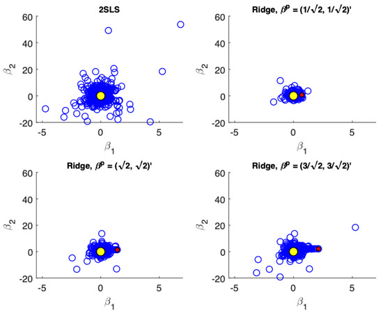
Figure 1. Scatter plots of the estimates from TSLS and ridge estimator with different priors when precision is low ($\delta =0.1$) and sample size is small ($n=25$). Estimates, the true parameter value and prior values are represented by blue, yellow and red points respectively. The variance associated with TSLS estimates is much larger than the ridge estimates. The ridge estimator is biased toward the prior.

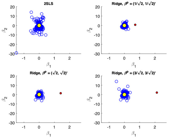
Figure 2. Scatter plots of the estimates from TSLS and ridge estimator with different priors when precision is low ($\delta =0.1$) and sample size is large ($n=500$). Estimates, the true parameter value and prior values are represented by blue, yellow and red points respectively. The variance associated with TSLS estimates is much larger than the ridge estimates. The ridge estimator is less biased towards the prior in the larger samples.

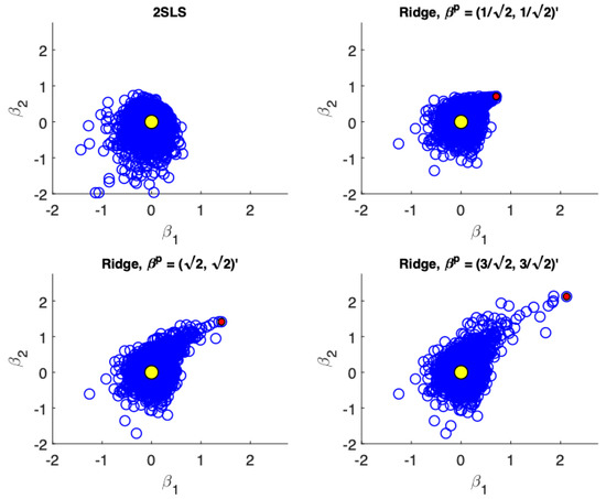
Figure 3. Scatter plots of the estimates from TSLS and ridge estimator with different priors when precision is high ($\delta =1$) and sample size is small ($n=25$). Estimates, the true parameter value and prior values are represented by blue, yellow and red points respectively. TSLS performance is much better in this setting. The variance reduction for the ridge estimator is not as dramatic.

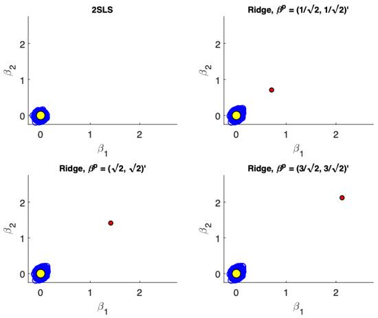
Figure 4. Scatter plots of the estimates from TSLS and ridge estimator with different priors when precision is high ($\delta =1$) and sample size is large ($n=500$). Estimates, the true parameter value and prior values are represented by blue, yellow and red points respectively. The TSLS estimates outperform the ridge estimators which is demonstrated by marginally larger clouds which are slightly off-center from the true parameter values for the ridge estimators. However, the ridge estimator using different priors is still competitive.

Table 3, summarizes the distribution of the estimated regularization parameter $\widehat{\alpha }$ for different precision levels, sample sizes and prior values. Recall Theorem 1 implies the asymptotic distribution will be a mixed distribution with some discrete mass at $\alpha =0.$ Table 3 reports the proportion of cases which correspond to “no regularization” ($\widehat{\alpha }=0$), “infinite regularization” ($\widehat{\alpha }={10}^7\approx \infty$) and “some regularization” ($\widehat{\alpha }\in (0,{10}^7)$). In all cases, there is a substantial mass of the distribution concentrated at $\widehat{\alpha }=0$. On the other hand we note that except in the cases where the prior is located at the true parameter value, there is no mass concentrated at $\widehat{\alpha }\approx \infty$. We see some interesting variations corresponding to different prior values. In low precision settings (particularly $\delta =0.1$), keeping sample size fixed, as the prior moves away from the true value, the proportion of cases with “no regularization” increases whereas the proportion of cases with “some regularization” falls. Similarly for high precision settings (particularly $\delta =1$), as the sample size increases, the proportion of cases with “no regularization” increases whereas the proportion of cases with “some regularization” falls. In this table we also present results for large sample sizes of $n=$ 10,000, which demonstrate that the mass at $\widehat{\alpha }=0$ approaches $50\%$ asymptotically, as predicted by Theorem 1. Distributions of $\widehat{\alpha }$ for large sample sizes of $n=$ 10,000 via histograms are presented in Figure 5.

Table 3. Distribution of regularization parameter $\widehat{\alpha }$. The mixed distribution associated with the finite samples is in agreement with the nonstandard asymptotic distribution given in Theorem 1. The proportion of cases with “no regularization” ($\widehat{\alpha }=0$), “some regularization” ($\widehat{\alpha }\in (0,{10}^7)$) and “infinite regularization” ($\widehat{\alpha }={10}^7\approx \infty$) are presented. For all cases, there is a substantial mass of the distribution concentrated at $\widehat{\alpha }=0$. On the other hand, there is no mass concentrated at $\widehat{\alpha }\approx \infty$except in very small samples of $n=25$. As predicted by Theorem 1, the mass at $\widehat{\alpha }=0$ is approaching $50\%$ asymptotically. Histograms for the large sample cases of $n=$ 10,000 are presented in Figure 5.

$\mathit{\delta }$	n	${\mathit{\beta }}^{\mathit{p}}={(1/\sqrt{2},1/\sqrt{2})}^{\prime }$			${\mathit{\beta }}^{\mathit{p}}={(\sqrt{2},\sqrt{2})}^{\prime }$			${\mathit{\beta }}^{\mathit{p}}={(3/\sqrt{2},3/\sqrt{2})}^{\prime }$
		$\widehat{\mathit{\alpha }}=0$	$\widehat{\mathit{\alpha }}\in (0,{10}^7)$	$\widehat{\mathit{\alpha }}={10}^7\approx \mathit{\infty }$	$\widehat{\mathit{\alpha }}=0$	$\widehat{\mathit{\alpha }}\in (0,{10}^7)$	$\widehat{\mathit{\alpha }}={10}^7$	$\widehat{\mathit{\alpha }}=0$	$\widehat{\mathit{\alpha }}\in (0,{10}^7)$	$\widehat{\mathit{\alpha }}={10}^7$
0.01	25	0.164	0.834	0.003	0.262	0.738	0.001	0.339	0.661	0.000
	50	0.166	0.834	0.000	0.275	0.725	0.000	0.354	0.646	0.000
	250	0.190	0.810	0.000	0.281	0.719	0.000	0.319	0.681	0.000
	500	0.220	0.780	0.000	0.285	0.715	0.000	0.302	0.698	0.000
	10,000	0.413	0.587	0.000	0.411	0.589	0.000	0.411	0.589	0.000
0.25	25	0.176	0.822	0.002	0.262	0.737	0.001	0.315	0.684	0.001
	50	0.184	0.816	0.000	0.263	0.737	0.000	0.299	0.701	0.000
	250	0.293	0.707	0.000	0.309	0.691	0.000	0.314	0.686	0.000
	500	0.346	0.654	0.000	0.354	0.646	0.000	0.354	0.646	0.000
	10,000	0.461	0.539	0.000	0.465	0.535	0.000	0.465	0.535	0.000
0.50	25	0.216	0.780	0.004	0.262	0.737	0.001	0.284	0.716	0.000
	50	0.255	0.745	0.000	0.284	0.716	0.000	0.294	0.706	0.000
	250	0.369	0.631	0.000	0.374	0.626	0.000	0.376	0.624	0.000
	500	0.412	0.588	0.000	0.415	0.585	0.000	0.417	0.583	0.000
	10,000	0.463	0.537	0.000	0.467	0.533	0.000	0.466	0.534	0.000
1.00	25	0.287	0.708	0.005	0.310	0.689	0.001	0.318	0.681	0.000
	50	0.333	0.667	0.000	0.346	0.654	0.000	0.351	0.649	0.000
	250	0.413	0.587	0.000	0.418	0.582	0.000	0.419	0.581	0.000
	500	0.439	0.561	0.000	0.443	0.557	0.000	0.442	0.558	0.000
	10,000	0.474	0.526	0.000	0.478	0.522	0.000	0.477	0.523	0.000

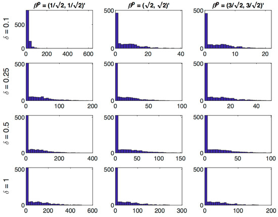
Figure 5. This figure plots the histogram of estimated regularization parameter $\widehat{\alpha }$ when $n=$ 10,000 for all precision parameters and all priors considered in the simulations. The total number of simulations to generate each of these plots is $N=1000$. As predicted by Theorem 1, the mass at $\widehat{\alpha }=0$ is approaching $50\%$ asymptotically. Distributions of $\widehat{\alpha }$ values for all cases considered are presented in Table 3.

Table 4 presents summaries of the smallest singular value of the matrix8$\left(\frac{-X^{\prime }Z}{n}\right)$ for different values of $\delta$ and n. The estimated asymptotic standard deviation is inversely related to the smallest singular value, or equivalently smaller singular values are associated with flatter objective functions at their minimum values. As the precision parameter increases from $\delta =0.1$ to $\delta =1$, the mean of the smallest singular value increases. As the sample size increases, the variance of the smallest singular values decreases.

Table 4. Summary statistics of the smallest singular value for the matrix $\left(-\frac{X^{\prime }Z}{n}\right)$ corresponding to different precision parameter values $\delta$ and sample sizes n, using 10,000 samples each. As the precision parameters increase from $\delta =0.1$ to $\delta =1$, the mean of the smallest singular value increases. As sample sizes increase from $n=25$ to $n=$ 10,000, the spread in the smallest singular value decreases.

$\mathit{\delta }$	n	Mean	Std Dev	1st Quartile	Median	3rd Quartile
0.10	25	0.25	0.14	0.14	0.23	0.33
	50	0.19	0.10	0.12	0.18	0.26
	250	0.12	0.05	0.08	0.12	0.16
	500	0.11	0.04	0.08	0.11	0.14
	2500	0.10	0.02	0.09	0.10	0.12
	5000	0.10	0.01	0.09	0.10	0.11
	10,000	0.10	0.01	0.09	0.10	0.11
0.25	25	0.32	0.17	0.19	0.30	0.42
	50	0.28	0.13	0.19	0.27	0.37
	250	0.26	0.07	0.21	0.26	0.30
	500	0.25	0.05	0.22	0.25	0.29
	2500	0.25	0.02	0.24	0.25	0.26
	5000	0.25	0.01	0.24	0.25	0.26
	10,000	0.25	0.01	0.24	0.25	0.26
0.50	25	0.50	0.21	0.35	0.48	0.63
	50	0.50	0.17	0.39	0.49	0.61
	250	0.50	0.08	0.45	0.50	0.55
	500	0.50	0.05	0.46	0.50	0.54
	2500	0.50	0.02	0.48	0.50	0.52
	5000	0.50	0.02	0.49	0.50	0.51
	10,000	0.50	0.01	0.49	0.50	0.51
1.00	25	0.86	0.27	0.67	0.85	1.03
	50	0.92	0.21	0.77	0.91	1.05
	250	0.98	0.10	0.91	0.98	1.05
	500	0.99	0.08	0.94	0.99	1.04
	2500	1.00	0.03	0.98	1.00	1.02
	5000	1.00	0.02	0.98	1.00	1.02
	10,000	1.00	0.02	0.99	1.00	1.01

5. Returns to Education

This section revisits the question of returns to schooling in Angrist and Krueger (1991). The key insight of that paper was the use of quarter of birth indicator variables as instruments to uniquely identify the impact of years of education on wages. The data are Public use Micro Sample of the 1980 U.S. Census and includes men born between 1920 and 1949 with positive earnings in 1979 and no missing observations. The sample is divided into three data sets, one for each decade. The empirical results are summarized in Table 5.

Table 5. Effect of years of education on the log of weekly earnings.

	1920–1929	1930–1939	1940–1949
OLS	0.070	0.063	0.052
TSLS	0.058	0.099	−0.073
Ridge	0.027	0.066	0.001
First stage F-test	38.3	30.5	26.3
Overidentification, Basmann	0.776	2.321	9.693
{p-value}	{0.679}	{0.313}	{0.008}
${\lambda }_{\min }$	3.3 × 10${}^{-6}$	1.3 × 10${}^{-5}$	6.6 × 10${}^{-7}$
Condition Number	4.1 × 10${}^7$	1.2 × 10${}^7$	2.8 × 10${}^8$
Sample size, n	247,199	329,509	486,926

The specification explains the log of weekly wages with the years of education; with race, standard metropolitan statistical area, marital status, region dummies, and year of birth dummies as controls9. The same data set was used in (Staiger and Stock 1997) which focused on weak instruments using the quarter of birth interacted with year of birth to create 30 instruments. To avoid weak instruments, we restrict attention to the quarter of birth dummy variables as instruments. This gives three instruments for years of education. The resulting first stage F-tests give no indication of weak instruments. The appropriateness of the specification is tested with the Basmann test for overidentify restrictions. The specification is not rejected for the 1920s and 1930s. However, the specification is rejected for the 1940s.

Each sample is split into a training sample with $\tau =0.7$ and a testing sample. The empirical results will be sensitive to this randomization. For each decade, the data was read into R from the Stata data set from the Angrist Data Archive at MIT, dplyr was used to filter the data for each decade and the random seed was set in R with “set.seed(12345)”. The samples have hundreds of thousands of observations, n, with 22 parameters estimated. However, there are precision problems with these estimates. As noted above in Section 2, the precision can be judged by the magnitude of the smallest eigenvalue of the second derivative of the objective function at the TSLS estimate for the entire sample, these are denoted ${\lambda }_{\min }$. The precision can also be judged with the condition number for the second derivatives which varies between 12 million and 282 million.

The prior for the ridge estimates was set empirically to judge the variability in the parameter estimates in the least informative dimension of the parameter space. The prior was set at four times the eigenvector associated with the smallest eigenvalue of the second derivative of the TSLS objective function for the training sample. This is moving four unit lengths away from the TSLS estimate in the flattest (least informative) direction. The ridge estimator is then defined by the value of $\alpha$ that minimizes the TSLS objective function using the test sample.

Even with the large sample sizes, the prior impacts the estimates. For the 1930s and 1940s the ridge estimate is between the OLS and the TSLS estimates. For the 1920s the ridge estimate is below both the TSLS estimate and the OLS estimate.

A final simulation exercise compares TSLS estimates with ridge estimates using the Angrist and Krueger (1991) data. As above the specification explains the log of weekly wages with the years of education; with race, standard metropolitan statistical area, marital status, region dummies, and year of birth dummies as controls. The quarter of birth dummies provide three instruments for years of education. Using the parameter estimates obtained by running the TSLS estimation on the entire sample from 1930s we obtain residuals $\widehat{u}$ and $\widehat{\epsilon }$ and their estimated covariance matrix. We then draw $N=$ 10,000 random samples of size n with replacement for the instruments and control variables and use these along with the full sample parameter estimates and error covariance to obtain simulated values of years of education and log of weekly wages.

TSLS and ridge estimates are obtained for each random sample and compared on the basis of bias, standard deviation and root mean square error (RMSE). For the ridge estimates each sample is split into a training sample with $\tau =0.7$ and a testing sample. Priors for all parameters are set to ${\widehat{\beta }}_{IV,train}$ i.e., the TSLS parameter estimate using only the training sample, except the parameter corresponding to returns to education. Three priors are considered for the returns to education parameter: ${\beta }_{edu}^p=\frac{1}{2}\left({\widehat{\beta }}_{edu,train}^{IV}\right)$, ${\beta }_{edu}^p=\left({\widehat{\beta }}_{edu,train}^{IV}\right)$ and ${\beta }_{edu}^p=2\left({\widehat{\beta }}_{edu,train}^{IV}\right)$. Results presented in Table 6 demonstrate that for the smallest sample size of n = 1000 ridge estimates corresponding to all three priors produce lower RMSE values for the parameter of interest compared to TSLS. On the other hand for the larger sample size of $n=$ 100,000 TSLS estimates produce lower RMSE values compared to ridge estimates for all three priors.

Table 6. Simulation results using returns to education data.

Prior	Sample Size	Estimator	Bias	SD	RMSE
${\beta }_{edu}^p=\frac{1}{2}\left({\widehat{\beta }}_{edu,train}^{IV}\right)$	1000	TSLS	$-0.032$	$0.185$	$0.188$
		Ridge	$-0.027$	$0.164$	$\mathbf{0}.\mathbf{166}$
	100,000	TSLS	$-0.001$	$0.039$	$\mathbf{0}.\mathbf{039}$
		Ridge	$-0.0003$	$0.058$	$0.058$
${\beta }_{edu}^p=\left({\widehat{\beta }}_{edu,train}^{IV}\right)$	1000	TSLS	$-0.032$	$0.192$	$0.194$
		Ridge	$-0.026$	$0.166$	$\mathbf{0}.\mathbf{168}$
	100,000	TSLS	$-0.002$	$0.039$	$\mathbf{0}.\mathbf{039}$
		Ridge	$-0.004$	$0.062$	$0.062$
${\beta }_{edu}^p=2\left({\widehat{\beta }}_{edu,train}^{IV}\right)$	1000	TSLS	$-0.036$	$0.181$	$0.184$
		Ridge	$-0.023$	$0.134$	$\mathbf{0}.\mathbf{136}$
	100,000	TSLS	$-0.001$	$0.038$	$\mathbf{0}.\mathbf{038}$
		Ridge	$-0.007$	$0.050$	$0.051$

6. Conclusions

The asymptotic distribution of the ridge estimator when the tuning parameter is selected with a test sample has been characterized. This estimator incorporates a non-zero prior and allows the non-negative tuning parameter to be zero. The resulting asymptotic distribution is a mixture with discrete mass on zero for the tuning parameter, a novel result, which follows from the true value of the tuning parameter lying on the boundary of the parameter space.

Simulations demonstrate where the ridge estimator produced lower MSE than the TSLS estimator, specifically when model precision is low, particularly in smaller samples and often even in larger samples. Where the TSLS estimator has lower MSE, particularly when precision is high, the ridge estimator remains competitive. As an empirical application, we have applied this procedure to the returns from education dataset used in (Angrist and Krueger 1991). Importantly, even with over 200,000 observations, the prior still influences the point estimates.

The ridge estimator will be particularly useful in addressing applied empirical questions where TSLS is appropriate but the available data suffers from low precision or where the sample size available is small. The characterization the asymptotic distribution of the ridge estimator also provides a useful framework for other estimators that involve tuning parameters.

Extensions and improvements of the approach are worthwhile to pursue. Different loss functions can be applied to the test sample (e.g., k-fold cross validation), we can allow for multiple tuning parameters, consider models without a closed form solution, allow the number of covariates to grow with the sample size, allow the number of tuning parameters to grow with the sample size, consider situation with weak instruments or nearly weak instruments, allow other penalty terms such as the LASSO or elastic-net.

References

- Andrews, Donald W. K. 2002. Generalized method of moments estimation when a parameter is on a boundary. Journal of Business & Economic Statistics 20: 530–44. [Google Scholar]
- Angrist, Joshua D., and Alan B. Krueger. 1991. Does compulsory school attendance affect schooling and earnings? The Quarterly Journal of Economics 106: 979–1014. [Google Scholar] [CrossRef]
- Antoine, Bertille, and Eric Renault. 2009. Efficient gmm with nearly-weak instruments. The Econometrics Journal 12: S135–S171. [Google Scholar] [CrossRef]
- Bengio, Yoshua. 2000. Gradient-based optimization of hyperparameters. Neural Computation 12: 1889–900. [Google Scholar] [CrossRef] [PubMed]
- Bickel, Peter J., Bo Li, Alexandre B. Tsybakov, Sara A. van de Geer, Bin Yu, Teófilo Valdés, Carlos Rivero, Jianqing Fan, and Aad van der Vaart. 2006. Regularization in statistics. Test 15: 271–344. [Google Scholar] [CrossRef]
- Carrasco, Marine, and Guy Tchuente. 2016. Efficient estimation with many weak instruments using regularization techniques. Econometric Reviews 35: 1609–37. [Google Scholar] [CrossRef]
- Carrasco, Marine, and Jean-Pierre Florens. 2000. Generalization of gmm to a continuum of moment conditions. Econometric Theory 16: 797–834. [Google Scholar] [CrossRef]
- Carrasco, Marine, Jean-Pierre Florens, and Eric Renault. 2007. Linear inverse problems in structural econometrics estimation based on spectral decomposition and regularization. Handbook of Econometrics 6: 5633–751. [Google Scholar]
- Carrasco, Marine. 2012. A regularization approach to the many instruments problem. Journal of Econometrics 170: 383–98. [Google Scholar] [CrossRef]
- Chen, Chen, Min Ren, Min Zhang, and Dabao Zhang. 2018. A two-stage penalized least squares method for constructing large systems of structural equations. Journal of Machine Learning Research 19: 40–73. [Google Scholar]
- Dorugade, Ashok Vithoba. 2014. New ridge parameters for ridge regression. Journal of the Association of Arab Universities for Basic and Applied Sciences 15: 94–99. [Google Scholar] [CrossRef]
- Firinguetti, Luis, and Gladys Bobadilla. 2011. Asymptotic confidence intervals in ridge regression based on the edgeworth expansion. Statistical Papers 52: 287–307. [Google Scholar] [CrossRef]
- Habibnia, Ali, and Esfandiar Maasoumi. 2019. Forecasting in big data environments: An adaptable and automated shrinkage estimation of neural networks (aashnet). arXiv arXiv:1904.11145. [Google Scholar]
- Hastie, Trevor, Robert Tibshirani, and Jerome Friedman. 2009. Unsupervised learning. In The Elements of Statistical Learning. New York: Springer, pp. 485–585. [Google Scholar]
- Hoerl, Arthur E., and Robert W. Kennard. 1970. Ridge regression: Biased estimation for nonorthogonal problems. Technometrics 12: 55–67. [Google Scholar] [CrossRef]
- Hoerl, Arthur E., Robert W. Kannard, and Kent F. Baldwin. 1975. Ridge regression: Some simulations. Communications in Statistics 4: 105–23. [Google Scholar] [CrossRef]
- Ichimura, Hidehiko. 1993. Semiparametric least squares (SLS) and weighted SLS estimation of single-index models. Journal of Econometrics 58: 71–120. [Google Scholar] [CrossRef]
- Larsen, Jan, Lars Kai Hansen, Claus Svarer, and Børje Ola Mattias Ohlsson. 1996. Design and regularization of neural networks: The optimal use of a validation set. Papaer presented at the 1996 IEEE Signal Processing Society Workshop, Kyoto, Japan, September 4–6; pp. 62–71. [Google Scholar] [CrossRef]
- Lawless, J. F., and P. Wang. 1976. A simulation study of ridge and other regression estimators. Communications in Statistics - Theory and Methods 5: 307–23. [Google Scholar] [CrossRef]
- Leeb, Hannes, and Benedikt M. Pötscher. 2005. Model selection and inference: Facts and fiction. Econometric Theory 21: 21–59. [Google Scholar] [CrossRef]
- Lin, Wei, Rui Feng, and Hongzhe Li. 2015. Regularization methods for high-dimensional instrumental variables regression with an application to genetical genomics. Journal of the American Statistical Association 110: 270–88. [Google Scholar] [CrossRef]
- Maclaurin, Dougal, David Duvenaud, and Ryan P. Adams. 2015. Gradient-based hyperparameter optimization through reversible learning. Paper presented at the 32nd International Conference on International Conference on Machine Learning—Volume 37, ICML’15, Lille, France, July 7–9; pp. 2113–22. [Google Scholar]
- Montgomery, Douglas C., Elizabeth A. Peck, and G. Geoffrey Vining. 2012. Introduction to Linear Regression Analysis. Wiley Series in Probability and Statistics; New York: Wiley. [Google Scholar]
- Sanderson, Eleanor, and Frank Windmeijer. 2016. A weak instrument f-test in linear iv models with multiple endogenous variables. Journal of Econometrics 190: 212–21. [Google Scholar] [CrossRef]
- Staiger, Douglas, and James H. Stock. 1997. Instrumental Variables Regression with Weak Instruments. Econometrica 65: 557–86. [Google Scholar] [CrossRef]
- Theobald, Chris M. 1974. Generalizations of mean square error applied to ridge regression. Journal of the Royal Statistical Society. Series B (Methodological) 36: 103–6. [Google Scholar] [CrossRef]
- Zhu, Ying. 2018. Sparse linear models and l1-regularized 2SLS with high-dimensional endogenous regressors and instruments. Journal of Econometrics 202: 196–213. [Google Scholar] [CrossRef]