1. Introduction
Inequality indices expressed as functions of the cumulative distribution function (CDF) are routinely used in studies that quantify inequality in self-assessed health, happiness, and other life satisfaction variables that are collected in the form of ordered response data. The large sample distribution of inequality indices of the CDF has been obtained by
Abul Naga and Stapenhurst (
2015). It is, however, an open question as to how reliable the adoption of the large sample distribution in testing hypotheses in applied work involving finite samples sizes is. Such an investigation (the first of this kind according to our best knowledge) is the main purpose of this paper. The focus of our investigation will be the Alphabeta family of inequality indices (
Abul Naga and Yalcin 2008) further extended by
Kobus and Milos (
2012). This family of indices has been associated with an important empirical literature (
Dutta and Foster 2013;
Jones et al. 2011;
Madden 2010;
Arrighi et al. 2015). This research is motivated by an important body of work, reviewed in
Cowell and Flachaire (
2015);
Davidson and Duclos (
2013), that documents poor finite sample performance of the
t-statistic of income inequality measures.
The inequality indices we investigate in this paper are smooth statistics of multinomial distributions. It is well known that for smooth statistics of multinomial distributions, the normal approximation provided by the central limit theorem is generally very accurate as sample size increases with the number of probability categories fixed, and as long as the underlying probability distribution lies in the interior of its parameter space.
1Nonetheless, there are several reasons a priori why we may want to consider undertaking bootstrap type inference for inequality indices defined on ordered response data. Firstly, we note that such indices are typically non-linear functions. The analytical calculation of their standard errors involves linearization using the
delta method.
Davison and Hinkley (
1997, p. 16) argue that simulation methods in practice can provide more accurate estimates of the distribution of test statistics than analytical methods that rely on the delta method. Also, under certain regularity assumptions, statistical theory will always recommend bootstrap inference over asymptotic tests in the context of
asymptotically pivotal test statistics and in presence of finite samples (
Horowitz 2001). Furthermore, in the income inequality literature, bootstrap methods often prove useful in cases where the exact distribution of the test is very complicated to obtain analytically (e.g.,
Barret et al. 2014).
Bootstrap methods, however, need not always be recommended over asymptotic inference in all sampling contexts. For instance,
Athreya (
1987) among others shows that bootstrap methods may fail when resampling occurs from long-tailed distributions. Likewise, in the context of income data,
Russell and Flachaire (
2007) show that the presence of outliers severely disrupts the performance of bootstrap inference in relation to income inequality measures.
A priori therefore, it is not clear which of bootstrap methods and asymptotic inference is to be preferred in economic investigations of inequality in relation to ordered response data. We therefore use Monte Carlo experiments to compare the empirical size and statistical power of asymptotic inference and the Studentized bootstrap test, in the context of a generic hypothesis test that a population has a given level of inequality
. We find that, in a broad variety of settings, both tests have similar rejection probabilities of true null hypotheses, and similar power. Nonetheless, the asymptotic test remains correctly sized in presence of certain types of severe class imbalances
2 exhibiting very low or very high levels of inequality, whereas the bootstrap test becomes somewhat oversized in these extreme settings. Given that the simulation results suggest that in practice the two tests perform very similarly, we are inclined to recommend the use of asymptotic inference in applied research involving the use of inequality indices of the cumulative distribution function.
The structure of the paper is as follows.
Section 2 presents the two families of inequality indices for ordered response data that will be the subject of our investigation.
Section 3 discusses the implementation of the Studentized bootstrap test in relation to the two families of inequality indices. In the discussion, we place particular emphasis on ensuring that sampling follows the two golden rules set out by
Davidson (
2007).
Section 4 discusses the methods of investigation used in exploring the comparative properties of the two tests.
Section 5 presents the results of the Monte Carlo simulations.
Section 6 presents a brief application, while
Section 7 concludes with a discussion of the limitations of the paper and directions for further research.
2. The Family of Inequality Indices
Let
denote a sample of observations on
k ordered categories of well-being (for example life satisfaction, self-reported health status or obesity status). Assume
individuals are reported to be in category 1,
individuals are reported to be in category
etc., and define
The resulting sample then follows a multinomial distribution. If
is drawn from an underlying population probability mass function (PMF)
the likelihood of
takes the form
We note that, in the context of multinomial sampling, the data counts
are jointly sufficient statistics for the sample
(see
Yalonetzky 2013, for further detail).
Inequality indices for ordered response data are often expressed in terms of the cumulative distribution associated with the sample We denote the sample’s frequency distribution where is the proportion of individuals who are in category We define as the resulting empirical cumulative distribution, where and we call X the empirical distribution function (EDF).
Let
denote the set of cumulative distributions defined over
k ordered categories of well-being. An inequality index for ordered response data is then some function defined on
with parameters reflecting some appropriately defined inequality aversion axiom and other ethical properties. First, to give an example of an inequality index that is linear in the cumulative distribution function, consider the family of sub-group decomposable indices of
Kobus and Milos (
2012):
Here
and
are parameter values chosen by the data analyst in order to reflect different social value judgements regarding inequality below, and above, the median category
m3 and
and
are normalization constants that insure that the index takes values in the unit interval
.
Likewise and are parameter values chosen to reflect social aversion to inequality below and above the median, and and are normalization constants. Note that the index is only linear in X in the specific case where and furthermore that for any distribution X.
The key property associated with the two families of inequality indices presented above is that they are increasing in median preserving spreads (
Allison and Foster 2004).
4 The above indices feature in studies aimed at quantifying health inequality in multiple country contexts (e.g.,
Jones et al. 2011;
Madden 2010) and also in simulating the envisaged effect of policy interventions on health inequality in the context of specific pathologies (e.g.,
Arrighi et al. 2015). They are also used in the quantification of happiness inequality in the United States (
Dutta and Foster 2013).
3. The Bootstrap and Asymptotic Test
The purpose of this section is to detail the procedures used to implement the asymptotic and bootstrap tests. We can think of a generic statistical test as a function where is a hypothesis being investigated and is a sample. The test function returns a p-value giving the lowest bound on the type-1 error rate for which we can reject the hypothesis of concern.
Let
denote the subset of
containing distributions with a median status
j. Then
and it is clear that
Accordingly, for some sample
of
n observations with EDF
drawn from a cumulative distribution function
, and some inequality index
consider testing the null hypothesis
We define the null space associated with this null hypothesis as the set of cumulative distribution functions
that exhibit the level of inequality
and whose median equals the median
m of the cumulative distribution
Let
denote any consistent estimator of the asymptotic variance of the inequality index. Conditional on the median category
an asymptotic test of the null hypothesis that
involves computing the test statistic
and approximating the exact distribution of
z under the null hypothesis by a standard normal distribution
5. Equivalently, for the asymptotic test, the critical values are obtained from the quantiles of the standard normal distribution.
As an alternative to asymptotic inference, bootstrap procedures simulate the distribution of the test via calculation of the test statistic in a large number of samples drawn from a distribution in the null space. Typically the null space (
5) contains many distributions, yet one way of ensuring a successful implementation of the bootstrap is to insure that sampling follows the related two golden rules (
Davidson 2007). The first of these rules requires that the data generating process underlying the bootstrap samples must belong to the model underlying the null hypothesis
The second golden rule requires that the data generating process underlying the bootstrap samples be obtained under the null hypothesis from an efficient estimation procedure.
Because the Maximum Likelihood estimator is generally efficient, it is of particular relevance, if possible, to use an ML procedure to select the underlying model of the null hypothesis, and to generate the bootstrap samples from this data generating process. This method of investigation, known as the
parametric bootstrap, ensures that both golden rules of bootstrap inference are satisfied (
Davidson 2007).
Associate with the estimation sample
the vector of responses
The ML estimator of the data generating process underlying
is obtained by maximizing the sample likelihood (
1) in the null space
Associate a probability mass function
f with the cumulative distribution
F. The ML estimator
of the data generating process underlying the null hypothesis of interest is then chosen as the maximizer of
in the null space
that is,
From here on, the ML estimator of the null hypothesis is used to generate
bootstrap samples
resulting in empirical distributions
and a sequence of test statistics
Here, is the empirical variance of the B values of the level of inequality. The sample quantiles of the B bootstrap statistics are used instead of the quantiles of the standard normal distribution in order to provide critical values for hypotheses tests related to the level of inequality in the underlying population.
4. Methods
Consider testing a null hypothesis of the generic form (4) using each of the asymptotic and bootstrap test discussed in the previous section. Call these two testing procedures and respectively. In this section we discuss how to use Monte Carlo simulation methods to evaluate the size and power properties of the asymptotic and bootstrap tests.
In order to obtain a good understanding of the comparative size and power properties of the two statistical tests, our interest in the Monte Carlo experiments will be to investigate for each of the two procedures, the effect of varying the parameters
F,
,
and
of the generic test (
4), in relation to different sample sizes. Our interest in examining the effect of sample size is to explore which of the two estimation procedures is to be recommended in applied work, involving small samples.
We explore changing the data generating process
F by varying its parameters, namely the number of response categories
k, the median response category
m6, and the underlying level of inequality
t. In varying these parameters of the DGP, we are particularly interested in investigating the effect of
severe class imbalances. The interest underlying DGPs exhibiting severe class imbalances, is that they allow the researcher to explore the effect of sampling near the boundary of the parameter space of the underlying multinomial population, where we expect the normal approximation of the distribution of the asymptotic test to be less accurate.
Varying
in the generic test (
4) allows us
to investigate test size (by setting
, where
t is the level of inequality associated with the DGP
F), and
to investigate statistical power (by setting
to be different from
t). We also explore variations in the null hypothesis (
4) by varying the inequality aversion parameters
and
of the underlying inequality index.
To provide a unified view of the scope of the envisaged simulation exercises, it is useful to consider a general Monte Carlo procedure as a method for studying the size and power properties a given test (in this paper we consider ) given a prescribed null hypothesis , a data generating process F, and a sample size n. A Monte-Carlo function is then an algorithmic procedure used to estimate, via simulation, the distribution of the resulting test statistic in a variety of contexts, such as those discussed above.
The strategy we pursue in the investigations is to define a baseline specification, and to explore variations from this benchmark case. The baseline case arises in relation to a sample size
n of 499 observations, a DGP associated with
socioeconomic classes, a median socioeconomic status
and a uniform probability mass function
(see
Table 1).
The inequality aversion parameters are set at the value and the resulting level of inequality is equal to The number B of bootstrap samples is set throughout equal to while the number of Monte Carlo samples is set to the value The appendix provides further detail about the DGPs used in the Monte Carlo investigations.
Our chosen method of summarizing the simulation results will be to rely on graphical methods developed by
Davidson and MacKinnon (
1998). Firstly, we shall report p
-value curves for both tests. The advantage of these graphical devices lies in allowing the researcher to investigate globally the size of tests, not just at key nominal values (such as
or
). We can furthermore identify a correctly sized test when its
p-value curve lies below the 45 degree line.To investigate power, we shall report
size–power curves. The advantage of the size–power curve is to quantify statistical power at a correct (i.e., consistently estimate) size, rather than nominal size. A test procedure
is more powerful than
in the context of a particular hypothesis of interest
, when the related size–power curve of
lies above the size–power curve pertaining to
.
5. Simulation Results
The focus in this section is on exploring the size and power properties of the asymptotic and bootstrap tests. With the exception of extreme cases of very low and very high inequality, we find that both tests are correctly sized in our investigations, and moreover, both tests have similar power even in the presence of small samples.
5.1. Sample Size
In the baseline specification of interest, we set the sample size at
and the other parameters of the DGP are chosen as indicated in
Table 1 and the
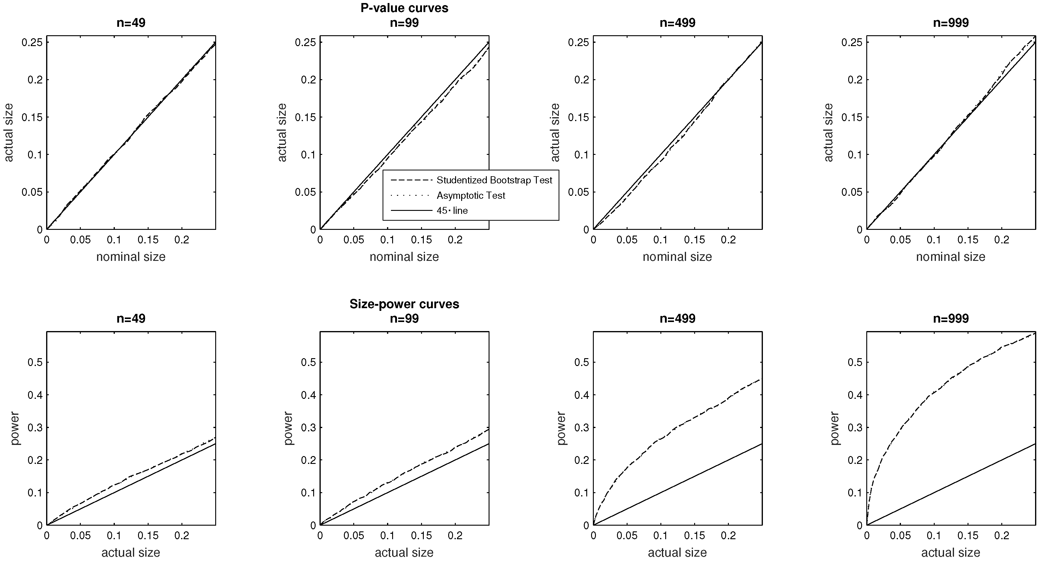
Appendix A of the paper. In the top panel of
Figure 1 we plot
p-value curves pertaining to both the asymptotic and bootstrap test, while the bottom panel plots size–power curves. The simulations pertain to sample sizes
,
,
(the baseline) and
We report on the horizontal axis of the
p-value curves nominal sizes from 0% to 25%. For the size–power curves, we report power over the same range of
actual sizes. For sample sizes of 49, 99 and 499 observations the
p-value curves lie below diagonal (45 degree) line, indicating that the tests are correctly sized. At nominal sizes exceeding 15%, we note nonetheless that the
p-value plots cross the diagonal axis in the context larger samples (
. Our central concern being the comparison of the relative performance of the two tests, we note that they perform equally well in terms of their
p-value curves.
Turning to the bottom panel where we report size–power curves, we observe that both testing methods also perform broadly similarly in terms of power, and the overall pattern is that power rises with sample size, as is of course expected to be the case.
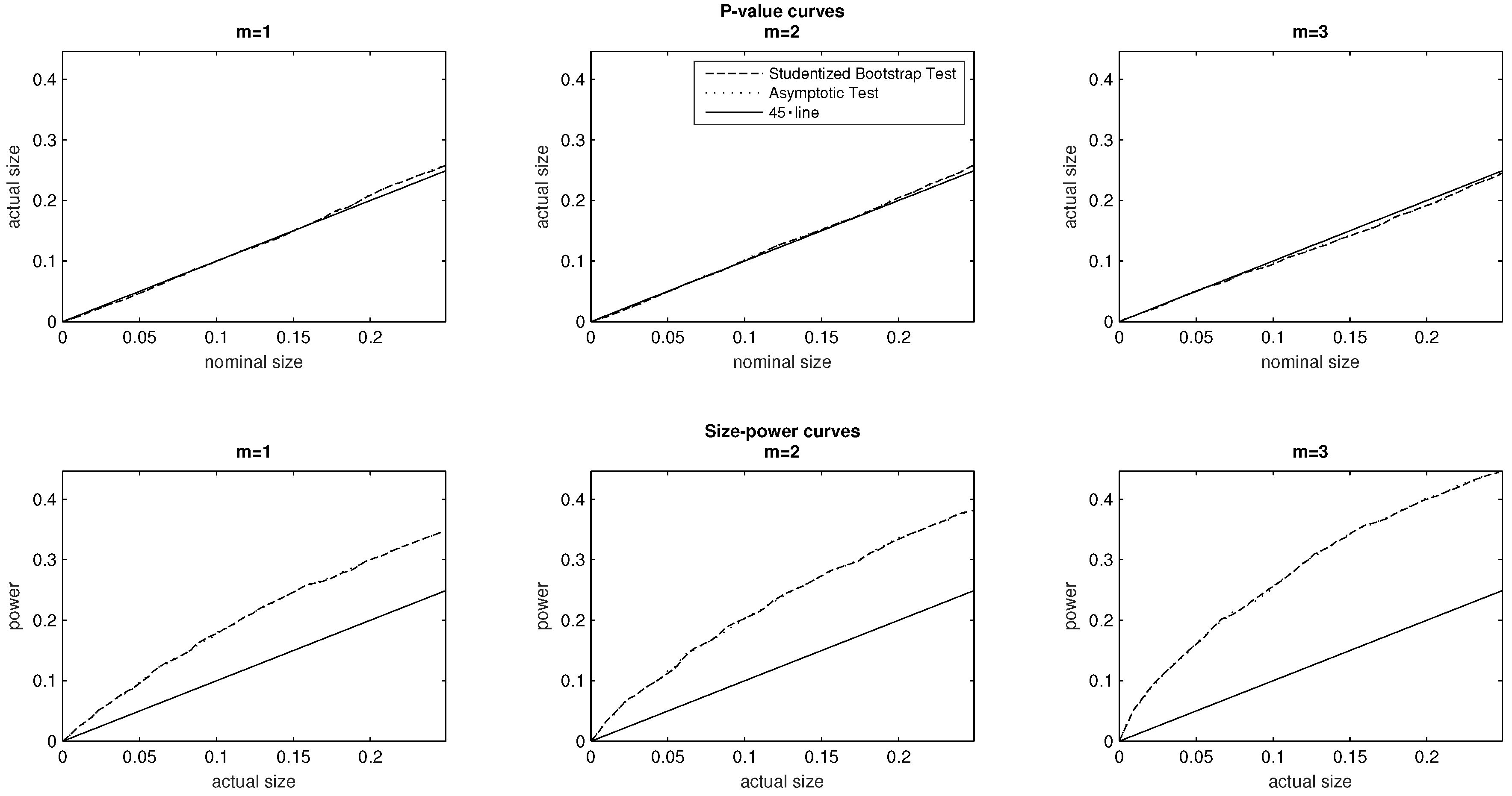
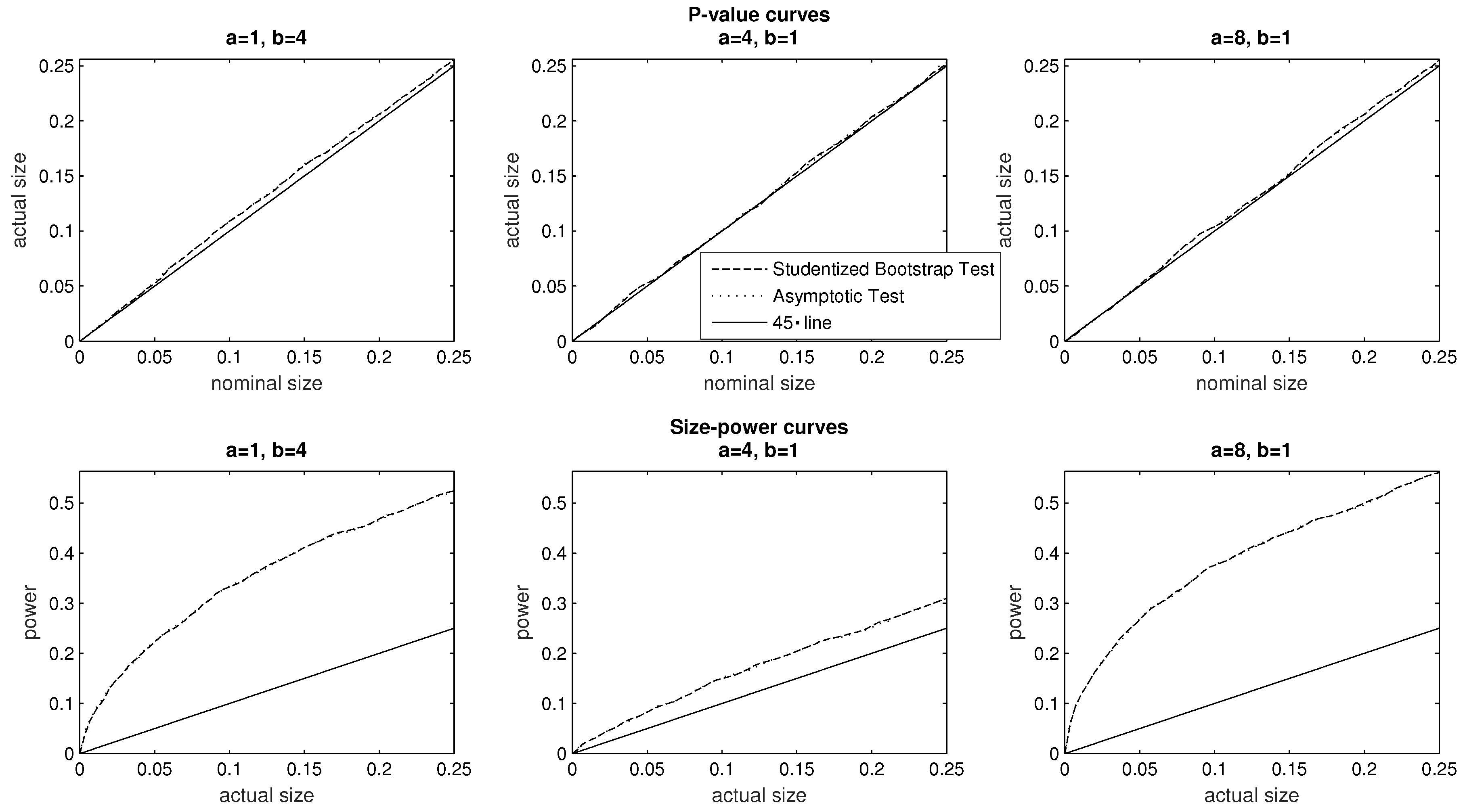
5.2. The Number of Response Categories
We are interested in exploring how the choice of DGP influences the relative performance of the asymptotic and Studentized bootstrap test. Our first investigation in this respect is to explore the effect of changing the number of response categories
The baseline specification chooses a uniform PMF defined on
socioeconomic categories, and we also examine DGPs pertaining to
and
For all three values of
the evidence plotted in the top panel of
Figure 2 supports the conclusion that both tests are correctly sized.
For a given sample size, it is not immediate to infer the effect of changing the number of response categories on the power of the tests. In the context of both tests, the findings of the bottom panel of
Figure 2 suggest, however, that other things equal, increasing
k from
to the baseline value
results in an increase of statistical power. The gain in power from increasing the number of response categories further to
is, however, less apparent in the context of both tests. In further investigations not reported in the paper, we explored the effect of further increasing
k (for a range of values from
to
for different sample sizes. We did not find however any general monotonic relation emerging between the number of response categories and statistical power in either of the asymptotic or Studentized bootstrap test.
5.3. The Median Response Category
By varying the median response category m of the distribution we can explore some parametric changes in the shape of the underlying DGP. We consider first a PMF with an associated median state We then somewhat reduce the mass at the bottom tail of the distribution (i.e., at the bottom socioeconomic status), and consider a PMF 10,000 with median state Finally, we use the baseline DGP to explore the effect of setting the median state at the value Note also that the three PMFs exhibit a level of inequality equal to (i.e., the baseline level), despite the different shapes of these probability mass functions and their varying median states.
For all three values of the median state
the evidence plotted in the top panel of
Figure 3 supports the conclusion that both tests are correctly sized. It is also the case that their
p-value curves broadly overlap. Turning to the size–power curves, the findings of the bottom panel of
Figure 3 suggest that upon varying the median response category, both tests perform equally well in terms of statistical power.
5.4. Inequality Aversion Parameters
We expect the asymptotic test to perform well in the context of a linear inequality index (i.e., when both inequality aversion parameters are set equal to one). When either inequality parameters are greater than unity, simulation methods in practice can provide more accurate estimates of the distribution of test statistics than analytical methods that rely on the
delta method (
Davison and Hinkley 1997, p. 16). For this reason, our interest here will be to investigate the practical advantage of adopting the Studentized bootstrap test, when the inequality aversion parameters are allowed to vary.
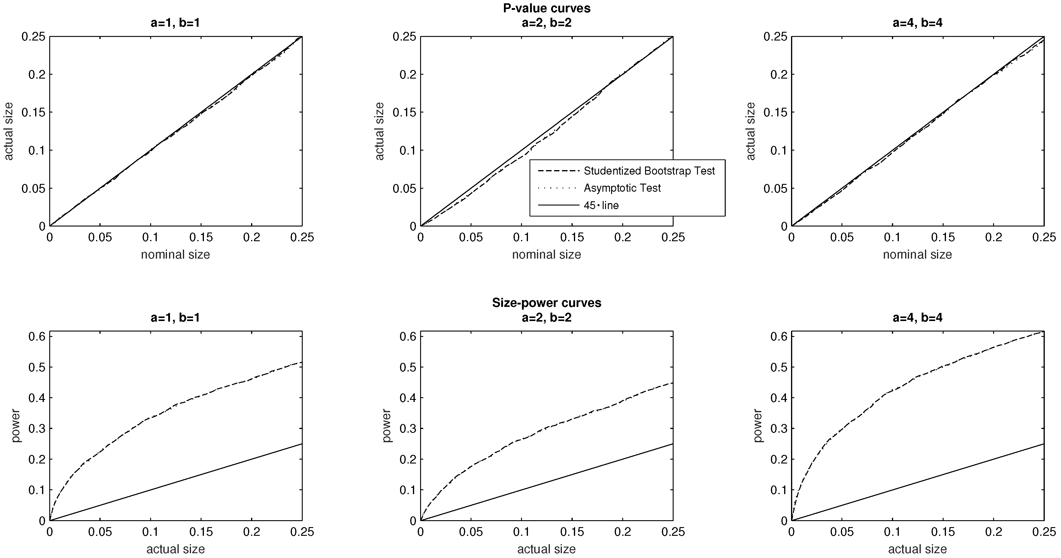
Specifically, in
Figure 4 we begin by setting the inequality aversion parameters to
The resulting inequality index being linear, is a member of the Kobus–Miłoś family (
2) of subgroup decomposable indices. We then examine the case pertaining to the baseline parameter values
followed by the case
For all three investigations, the evidence plotted in the top panel of
Figure 4 supports the conclusion that both tests are correctly sized, and the
p-value curves specific to each investigation broadly overlap. Turning to the size–power curves, the findings of the bottom panel of
Figure 4 suggest that the two tests exhibit broadly similar power for each pair of parameter values, and furthermore that the power of each given test is sensitive to the specification of the inequality index.
In the investigations of
Figure 5, we explore the effect of attaching different weight to the bottom and top tails of the distribution via setting
and
at different parameter values: a larger value of
renders the inequality index more sensitive to the bottom tail of the distribution, while increasing
makes the index more sensitive to the top tail of the distribution. We depict the
p-value and size–power curves of the two tests in relation to the following sequence of inequality aversion parameters:
and
For all three investigations, the evidence in the top panel of
Figure 5 supports the conclusion that both tests are moderately over-sized, while the
p-value curves of the two tests in each specific investigation broadly overlap. The bottom panel reveals that the power of the tests is sensitive to the specification of the inequality index. There is little to differentiate the asymptotic and Studentized bootstrap test in term of size–power curves, and, as in the findings of
Figure 4, we are led to conclude that the power of each test is sensitive to the choice of inequality aversion parameters.
5.5. Severe Class Imbalances
To investigate the effect of severe class imbalances, our strategy here is to generate a sequence of distributions that are ordered by the relation. That is, we consider a sequence of PMFs where for , is obtained from using a number of median preserving spreads. In increasing order, the level of inequality t associated with each of the distributions in the sequence equals , , , , and . We note here however that associated with the two polar cases of extreme equality and inequality are two PMFs that exhibit severe class imbalances: , and On the other hand, coincides with the PMF of the baseline model, which exhibits a property of extremely well balanced classes. There are two other PMFs in the sequence, and Both of and share a common median ( however exhibits a less balanced class structure than and furthermore lies at the boundary of the parameter space defining multinomial distributions.
We also consider a second sequence of PMFs ordered by the median preserving spreads relation, given by
where
replaces
and such that the level of inequality at
equals
. This new PMF,
is chosen to lie at the boundary between the subsets
and
pertaining to distributions with median states equal to 3 and 4 respectively.
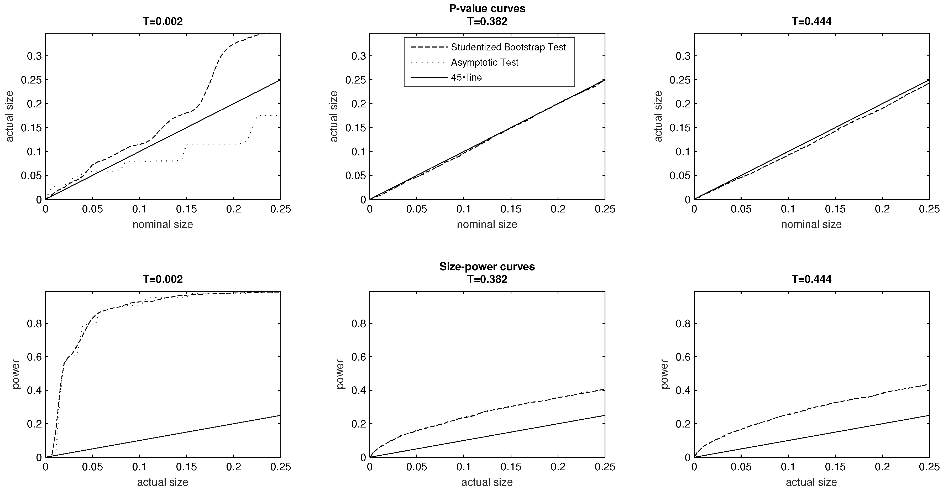
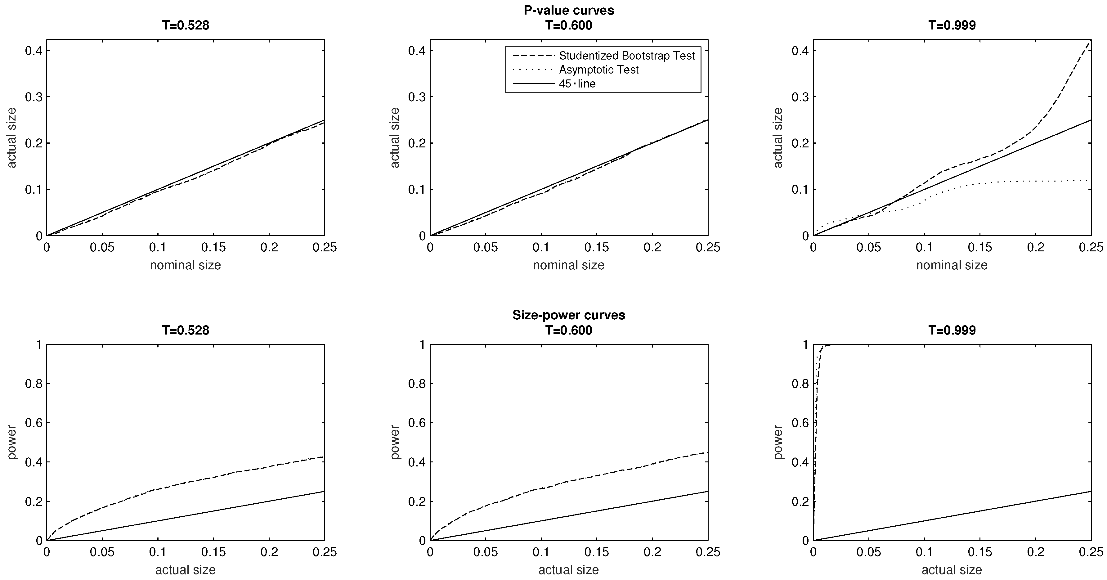
7The top panel of
Figure 6 provides
p-value plots for the tests associated with the (from left to right) the DGPs of
and
The PMF
chosen to exhibit severe class imbalances is of particular interest, as it generates marked differences in the
p-value curves associated with the asymptotic test and the Studentized bootstrap test. At low significance levels 0% to 5%, the asymptotic test is moderately oversized. We may however note that at higher significance levels (6% to 25%) the asymptotic test is correctly sized, rather than being oversized. The bootstrap test is oversized at all significance levels, and its size substantially exceeds that of the asymptotic test above the 4% significance level. It is equally important to observe that any differences between the
p-value curves of the two tests become hardly visible in relation to the DGPs associated with the PMFs
and
The bottom panel of
Figure 6 reports the size–power curves of the two tests in relation to the DGPs associated with
and
In the case of severe class imbalances (the DGP associated with
) the two tests exhibit very similar power, and the conclusion is similar when inequality rises in the case of
and
Figure 7 similarly plots
p-value and size–power curves for the DGPs associated with the remaining PMFs
and
In terms of test size and power, the plots of the top and bottom panel reveal that both the asymptotic and bootstrap test perform very similarly in relation to
and
Recalling that
is the uniform PMF of the baseline model, we do not find in this investigation that severe class balances lead to oversized tests, comparatively low power, or overall differences in the
p-value or size–power curves of the two tests.
As discussed above, the probability mass function
exhibits the polar case of high inequality
, and is associated with severe class imbalances. The findings in relation to the DGP associated with
are qualitatively similar to those of the DGP associated with
which exhibits the opposite polar case of low inequality. Here we find that at low significance levels (0% to 4%), the asymptotic test is moderately oversized. We may however note that at higher significance levels (5% to 25%) the asymptotic test is correctly sized. The bootstrap test remains correctly sized at significance levels 0% to 6% but then becomes (increasingly) oversized at all levels above the 7% significance level. Nonetheless, we do not find any substantial differences in the size–power curves of the two tests in the bottom panel of
Figure 7. What we can document, however, is that statistical power is considerably higher in the extreme cases of severe class imbalances than in the intermediate cases of the two sequences of PMFs, using either of the two tests.
6. An Illustrative Example
As an illustrative example, we return to the data application in
Abul Naga and Stapenhurst (
2015) pertaining to asymptotic inference in relation to the Alphabeta family of inequality indices (
3). These are data on five ordered nutritional health states from the Egyptian Integrated Household Survey of 1997–1999.
8 The data refer to two statistical areas of Northern Egypt (also known as
Lower Egypt), namely Metropolitan Lower Egypt (METLO) and Non-Metropolitan Lower Egypt (NMETLO). The resulting cumulative distributions are respectively
for the METLO data
and
for the NMETLO data
Note also that the median response category is
in both distributions. The data from the larger sample exhibit somewhat more class imbalances than the first sample, though neither sample exhibits the levels of class imbalances found to be problematic in the simulations of
Section 5.
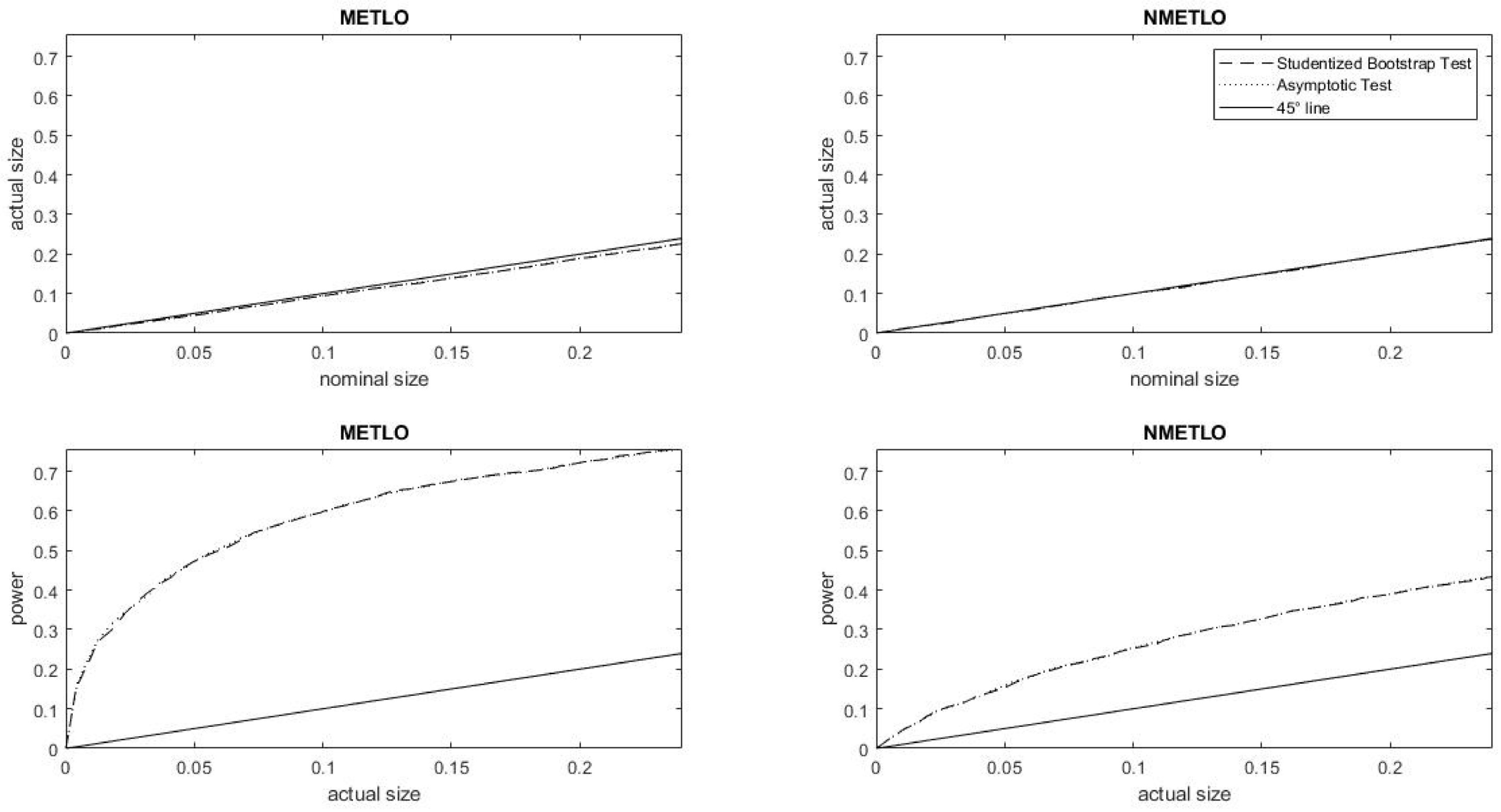
We begin by carrying out the same exercise as in
Section 5, for the empirical distribution functions of the data. Using the baseline values
of the inequality aversion parameters, inequality is calculated at
and
in respectively the Metropolitan (METLO) and Non-Metropolitan (NMETLO) samples. We next investigate a hypothesis that inequality in a given sample—computed at parameter values
—is equal to
(the level of inequality of the pooled sample, computed at the same parameter values.) On the basis of the simulations reported in the results section, we expect the asymptotic and bootstrap tests to exhibit very similar
p-value curves as well as size–power curves. Inspecting the related curves in
Figure 8, we find that this pattern indeed does emerge. It is worth noting however that the power of the test is considerably higher in the smaller METLO sample. This pattern is to be expected, as the hypothesized value of
is considerably closer to the level of inequality in the larger Non-Metropolitan sample
than it is in the Metropolitan Lower Egypt
We report these inequality computations pertaining to parameter values
in
Table 2, together with other computations of inequality in the two samples for various pairs of parameter values. Rows 4 and 5 of the Table furthermore report
p-values arising from the bootstrap test of the hypothesis that each of the respective samples has the same level of inequality
T of the combined sample. In the context of the computations pertaining to parameter values
both samples exhibit identical levels of inequality, a
figure, and hence the
p-values of both tests are equal to 1. We observe that it is also the case that for the other pairs of parameter values, the bootstrap test fails to reject at the 5% level the hypothesis that either of the two populations has a level of inequality equal to that of the combined sample. Nonetheless, we note that in the context of the computations pertaining to parameter values
, the test does reject at the
the hypothesis that METLO has the same level of inequality
as the combined sample (last column of the table).
In order to highlight one practical difference between the two tests, we calculate in rows 6 to 9 of
Table 2 the
confidence intervals for inequality in the two samples, using both bootstrap inference (the rows starting with
) and asymptotic inference (the rows starting with the cell
9. These intervals consist of all the levels of inequality that we would fail to reject at the 5% level. While the asymptotic inference confidence intervals are by construction symmetric about the sample value
of inequality, this symmetry need not arise in the context of the bootstrap confidence intervals. We find here that the bootstrap confidence intervals are generally larger than the asymptotic confidence intervals. These findings, obtained in the context of sample sizes of 100 to 500 observations, would suggest that the exact distribution of the alphabeta inequality index may exhibit thicker tails than those of the standard normal distribution.
7. Conclusions
We have used Monte Carlo experiments to compare the empirical size and statistical power of asymptotic inference and the Studentized bootstrap test. We have found that in all our investigations the asymptotic and bootstrap test exhibit very similar size–power curves. With the exception of extreme cases of very low and very high inequality, we also have found that both tests are correctly sized in our investigations. The experiments pertaining to extremely low and high levels of inequality (respective values of 0.002 and 0.999) present cases of several class imbalances in the underlying data generating process. In these two investigations, the asymptotic test remains correctly sized at all test sizes ranging between 0% and 25%, while the bootstrap test becomes increasingly oversized at all levels starting from the 6% value. Nonetheless, both tests remain correctly sized under other cases of severe class imbalances or other cases where the DGP lies at the boundary of the parameter space pertaining to multinomial distributions. Awaiting further investigations of this nature, given the numerical cost associated with implementing the bootstrap test, our broad recommendation to applied researchers would be to adopt asymptotic inference in the context of inequality indices defined on ordered response data. That is, the context of ordered response data would appear to be of a separate nature from income data, where asymptotic inference has been documented to often produce incorrectly sized tests.
These conclusions have been reached in the context of sampling where the population median, used in order to determine the functional form of the inequality index, was assumed to be known. It is therefore important in further investigations to develop a framework for exploring the performance of the two tests in sampling contexts where the median of the distribution is treated as a random quantity.
10


