State-Space Models on the Stiefel Manifold with a New Approach to Nonlinear Filtering

Abstract

We develop novel multivariate state-space models wherein the latent states evolve on the Stiefel manifold and follow a conditional matrix Langevin distribution. The latent states correspond to time-varying reduced rank parameter matrices, like the loadings in dynamic factor models and the parameters of cointegrating relations in vector error-correction models. The corresponding nonlinear filtering algorithms are developed and evaluated by means of simulation experiments.

1. Introduction

The coefficient matrix of explanatory variables in multivariate time series models can be rank deficient due to some modelling assumptions, and the parameter constancy of the rank deficient matrix may be questionable. This may happen, for example, in the factor model, which construct very few factors by using a large number of macroeconomic and financial predictors, while the factor loadings are suspect to be time-varying. Stock and Watson (2002) state that it is reasonable to suspect temporal instability taking place in factor loadings, and later Stock and Watson (2009) and Breitung and Eickmeier (2011) find empirical evidence of instability. Another setting where instability may arise is in cointegrating relations (see e.g., Bierens and Martins (2010)), hence in the the reduced rank cointegrating parameter matrix of a vector error-correction model.

There are solutions in the literature to the modelling of the temporal instability of reduced rank parameter matrices. Such parameters are typically regarded as unobserved random components and in most cases are modelled as random walks on a Euclidean space; see, for example, Del Negro and Otrok (2008) and Eickmeier et al. (2014). In these works, the noise component of the latent processes (factor loading) is assumed to have a diagonal covariance matrix in order to alleviate the computational complexity and make the estimation feasible, especially when the dimension of the system is high. However, the random walk assumption on the Euclidean space cannot guarantee the orthonormality of the factor loading (or cointegration) matrix, while this type of assumption identifies the loading (or cointegration) space. Hence, other identification restrictions on the Euclidean space are needed. Moreover, the diagonality of the error covariance matrix of the latent processes contradicts itself when a permutation of the variables is performed.

In this work, we develop new state-space models on the Stiefel manifold, which do not suffer from the problems on the Euclidean space. It is noteworthy that Chikuse (2006) also develops state-space models on the Stiefel manifold. The key difference between Chikuse (2006) and our work is that we keep the Euclidean space for the measurement evolution of the observable variables, while Chikuse (2006) puts them on the Stiefel manifold, which is not relevant for modelling economic time series. By specifying the time-varying reduced rank parameter matrices on the Stiefel manifold, their orthonormality is obtained by construction, and therefore their identification is guaranteed.

The corresponding recursive nonlinear filtering algorithms are developed to estimate the a posteriori distributions of the latent processes of the reduced rank matrices. By applying the matrix Langevin distribution on the a priori distributions of the latent processes, conjugate a posteriori distributions are achieved, which gives great convenience in the computational implementation of the filtering algorithms. The predictive step of the filtering requires solving an integral on the Stiefel manifold, which does not have a closed form. To compute this integral, we resort to a Laplace method.

The paper is organized as follows. Section 2 introduces the general framework of the vector models with time-varying reduced rank parameters. Two specific forms of the time-varying reduced rank parameters, which the paper is focused on, are given. Section 3 discusses some problems in the prevalent literature on modelling the time dependence of the time-varying reduced rank parameters, which underlie our modelling choices. Then, in Section 4, we present the novel state-space models on the Stiefel manifold. Section 5 presents the nonlinear filtering algorithms that we develop for the new state-space models. Section 6 presents several simulation based examples. Finally, Section 7 concludes and gives possible research extensions.

2. Vector Models with Time-Varying Reduced Rank Parameters

Consider the multivariate time series model with partly time-varying parameters

$${\mathit{y}}_t={\mathit{A}}_t{\mathit{x}}_t+\mathit{B}{\mathit{z}}_t+{\mathbf{\epsilon }}_t,t=1,\dots ,T,$$

(1)

where ${\mathit{y}}_t$ is a (column) vector of dependent variables of dimension p, ${\mathit{x}}_t$ and ${\mathit{z}}_t$ are vectors of explanatory variables of dimensions $q_1$ and $q_2$, ${\mathit{A}}_t$ and $\mathit{B}$ are $p\times q_1$ and $p\times q_2$ matrices of parameters, and ${\mathbf{\epsilon }}_t$ is a vector belonging to a white noise process of dimension p, with positive-definite covariance matrix $\mathsf{\Omega }$. For quasi-maximum likelihood estimation, we further assume that ${\mathbf{\epsilon }}_t\sim N_p(\mathbf{0},\mathsf{\Omega })$.

The distinction between ${\mathit{x}}_t$ and ${\mathit{z}}_t$ is introduced to separate the explanatory variables between those that have time-varying coefficients (${\mathit{A}}_t$) from those that have fixed coefficients ($\mathit{B}$). In the sequel, we always consider that ${\mathit{x}}_t$ is not void (i.e., $q_1>0$). The explanatory variables may contain lags of ${\mathit{y}}_t$, and the remaining stochastic elements (if any) of these vectors are assumed to be weakly exogenous. Equation (1) provides a general linear framework for modelling time-series observations with time-varying parameters, embedding multivariate regressions and vector autoregressions. For an exposition of the treatment of such a model using the Kalman filter, we refer to Chapter 13 of Hamilton (1994).

We assume furthermore that the time-varying parameter matrix ${\mathit{A}}_t$ has reduced rank $r<min(p,q_1)$. This assumption can be formalized by decomposing ${\mathit{A}}_t$ as ${\mathbf{\alpha }}_t{\mathbf{\beta }}_t^{\prime }$, where ${\mathbf{\alpha }}_t$ and ${\mathbf{\beta }}_t$ are $p\times r$ and $q_1\times r$ full rank matrices, respectively. If we allow both ${\mathbf{\alpha }}_t$ and ${\mathbf{\beta }}_t$ to be time-varying, the model is not well focused and hard to explain, and its identification is very difficult. Hence, we focus on the cases where either ${\mathbf{\alpha }}_t$ or ${\mathbf{\beta }}_t$ is time-varying, that is, on the following two cases:

$$\begin{array}{cc}\hfill \mathrm{Case}1:& {\mathit{A}}_t={\mathbf{\alpha }}_t{\mathbf{\beta }}^{\prime },\hfill \end{array}$$

(2)

$$\begin{array}{cc}\hfill \mathrm{Case}2:& {\mathit{A}}_t=\mathbf{\alpha }{\mathbf{\beta }}_t^{\prime }.\hfill \end{array}$$

(3)

Next, we explain how the two cases give interesting alternatives to modelling different kinds of temporal instability in parameters.

The case 1 model (Equations (1) and (2)) ensures that the subspace spanned by $\mathbf{\beta }$ is constant over time. This specification can be viewed as a cointegration model allowing for time-varying short-run adjustment coefficients (the entries of ${\mathbf{\alpha }}_t$) but with time-invariant long-run relations (cointegrating subspace). To see this, consider that model (1) corresponds to a vector error-correction form of a cointegrated vector autoregressive model of order k with ${\mathit{X}}_t$ as the dependent variables, if ${\mathit{y}}_t=\Delta {\mathit{X}}_t$, ${\mathit{x}}_t={\mathit{X}}_{t-1}$, ${\mathit{z}}_t$ contains $\Delta {\mathit{X}}_{t-i}$ for $i=1,\dots ,k-1$, as well as some predetermined variables. There are papers in the literature arguing that the temporal instability of the parameters in both stationary and non-stationary macroeconomic data does exist and cannot be overlooked. For example, Swanson (1998) and Rothman et al. (2001) give convincing examples in investigating the Granger causal relationship between money and output using a nonlinear vector error-correction model. They model the instability in $\mathbf{\alpha }$ by means of regime-switching mechanisms governed by some observable variable. An alternative to that modelling approach is to regard ${\mathbf{\alpha }}_t$ as a totally latent process.

The case 1 model also includes as a particular case the factor model with time-varying factor loadings. In the factor model context, the factors ${\mathit{f}}_t$ are extracted from a number of observable predictors ${\mathit{x}}_t$ by using the r linear combinations ${\mathit{f}}_t={\mathbf{\beta }}^{\prime }{\mathit{x}}_t$. Note that ${\mathit{f}}_t$ is latent since $\mathbf{\beta }$ is unknown. Then, the corresponding factor model (neglecting the $\mathit{B}{\mathit{z}}_t$ term) takes the form

$${\mathit{y}}_t={\mathbf{\alpha }}_t{\mathit{f}}_t+{\mathbf{\epsilon }}_t,$$

(4)

where ${\mathbf{\alpha }}_t$ is a matrix of the time-varying factor loadings. The representation is quite flexible in the sense that ${\mathit{y}}_t$ can be equal to ${\mathit{x}}_t$ and then we reach exactly the same representation as Stock and Watson (2002), but we also allow them to be distinct. In Stock and Watson (2002), the factor loading matrix $\mathbf{\alpha }$ is time-invariant and the identification is obtained by imposing the constraints $q_1\mathbf{\alpha }=\mathbf{\beta }$ and ${\mathbf{\alpha }}^{\prime }\mathbf{\beta }={\mathbf{\beta }}^{\prime }\mathbf{\alpha }={\mathbf{\alpha }}^{\prime }\mathbf{\alpha }/q_1=q_1{\mathbf{\beta }}^{\prime }\mathbf{\beta }={\mathit{I}}_r$. Notice that, if $\mathbf{\alpha }$ is time-varying but $\mathbf{\beta }$ time-invariant, these constraints cannot be imposed.

The case 2 model (Equations (1) and (3)) can be used to account for time-varying long-run relations in cointegrated time series, as ${\mathbf{\beta }}_t$ is changing. Bierens and Martins (2010) show that this may be the case for the long run purchasing power parity. In the case 2 model, there exist $p-r$ linearly independent vectors ${\mathbf{\alpha }}_{\perp }$ that span the left null space of $\mathbf{\alpha }$, such that ${\mathbf{\alpha }}_{\perp }^{\prime }{\mathit{A}}_t=\mathbf{0}$. Therefore, the case 2 model implies that the time-varying parameter matrix ${\mathbf{\beta }}_t$ vanishes in the structural vector model

$${\gamma }^{\prime }{\mathit{y}}_t={\gamma }^{\prime }\mathit{B}{\mathit{z}}_t+{\gamma }^{\prime }{\mathbf{\epsilon }}_t,$$

(5)

for any column vector $\gamma \in \mathfrak{sp}\left({\mathbf{\alpha }}_{\perp }\right)$, where $\mathfrak{sp}\left({\mathbf{\alpha }}_{\perp }\right)$ denotes the space spanned by ${\mathbf{\alpha }}_{\perp }$, thus implying that the temporal instability can be removed in the above way. Moreover, ${\mathit{x}}_t$ does not explain any variation of ${\gamma }^{\prime }{\mathit{y}}_t$.

Another possible application for the case 2 model is the instability in the factor composition. Considering the factor model ${\mathit{y}}_t=\mathbf{\alpha }{\mathit{f}}_t+{\mathbf{\epsilon }}_t$, with time-invariant factor loading $\mathbf{\alpha }$, the factor composition may be slightly evolving through ${\mathbf{\beta }}_t$ in ${\mathit{f}}_t={\mathbf{\beta }}_t^{\prime }{\mathit{x}}_t$.

3. Issues about the Specification of the Time-Varying Reduced Rank Parameter

In the previous section, we have introduced two models with time-varying reduced rank parameters. In this section, in order to motivate our choices presented in Section 4, we discuss the specification in the literature of the dynamic process governing the evolution of the time-varying parameters.

Since the sequences ${\mathbf{\alpha }}_t$ or ${\mathbf{\beta }}_t$ in the two cases are unobservable in practice, it is quite natural to write the two models into the state-space form with a measurement equation like (1) for the observable variables and transition equations for ${\mathbf{\alpha }}_t$ or ${\mathbf{\beta }}_t$. To build the time dependence in the sequences of ${\mathbf{\alpha }}_t$ or ${\mathbf{\beta }}_t$ is of great practical interest as it enables one to use the historical time series data for conditional forecasting, especially by using the prevalent state-space model based approach. How to model the evolution of these time-varying parameters, nevertheless, is an open issue and needs careful investigation. Almost all the works in the literature of time series analysis hitherto only deal with state-space models on the Euclidean space. See, for example, the books by Hannan (1970); Anderson (1971); Koopman (1974); Durbin and Koopman (2012); and more recently Casals et al. (2016).

Consider, for example, the factor model (4) with time-varying factor loading ${\mathbf{\alpha }}_t$, but notice that the following discussion can be easily adapted to the cointegration model, where only ${\mathbf{\beta }}_t$ is time-varying. The traditional state-space framework on the Euclidean space assumes that the elements of the time-varying matrix ${\mathbf{\alpha }}_t$ evolve like random walks on the Euclidean space, see for example Del Negro and Otrok (2008) and Eickmeier et al. (2014). That is,

$$\mathrm{vec}\left({\mathbf{\alpha }}_{t+1}\right)=\mathrm{vec}\left({\mathbf{\alpha }}_t\right)+{\mathbf{\eta }}_t,$$

(6)

where vec denotes the vectorization operator, and the sequence of ${\mathbf{\eta }}_t$ is assumed to be a Gaussian strong white noise process with constant positive definite covariance matrix ${\mathbf{\Sigma }}_{\eta }$. Thus, Labels (1) and (6) form a vector state-space model, and the Kalman filter technique can be applied for estimating ${\mathbf{\alpha }}_t$.

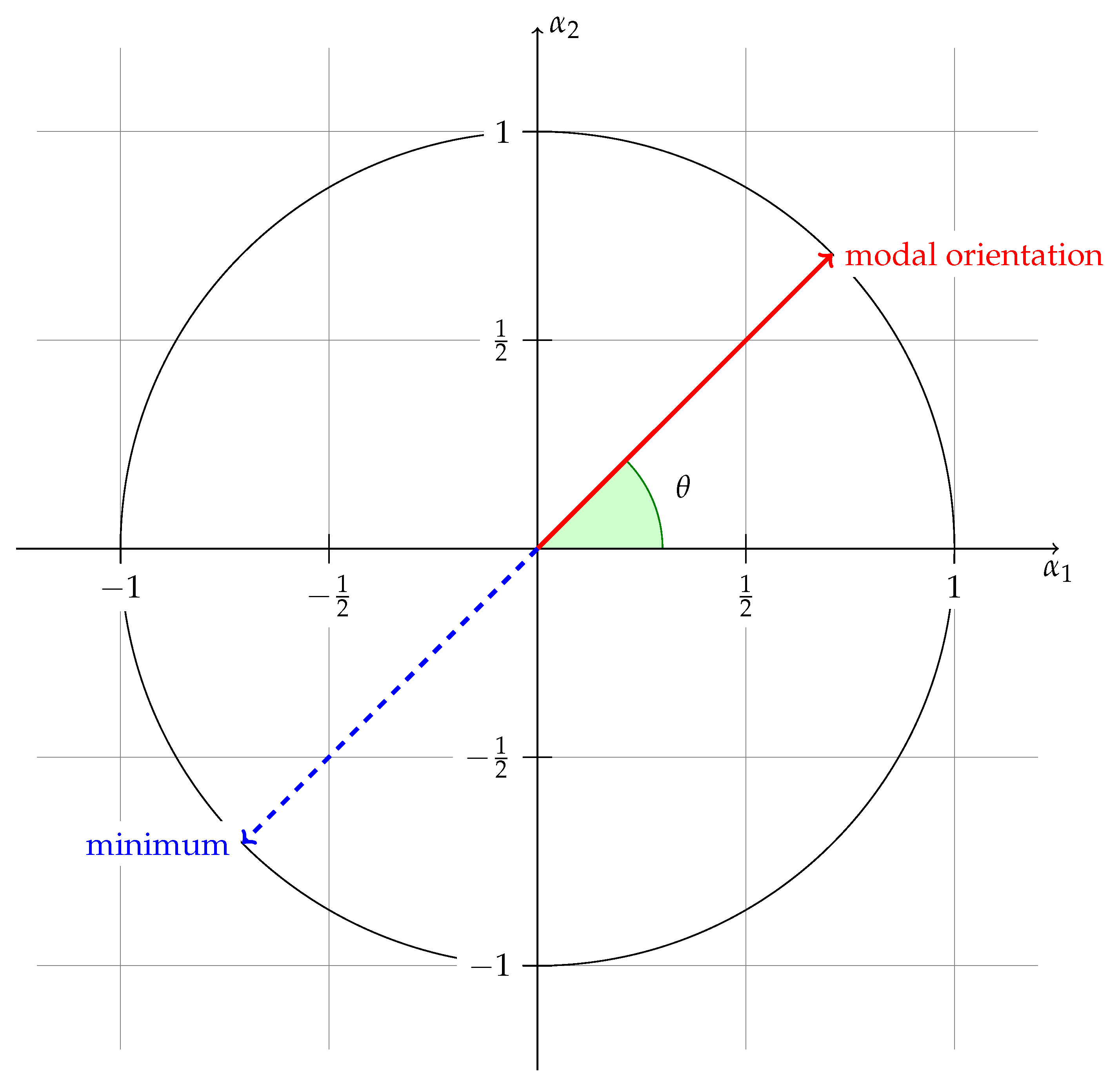
A first problem of the model (6) is that the latent random walk evolution on the Euclidean space is strange. Consider the special case $p=2$ and $r=1$: in Figure 1, points 1–3 are possible locations of the latent variable $\mathrm{vec}\left({\mathbf{\alpha }}_t\right)={({\alpha }_{1t},{\alpha }_{2t})}^{\prime }$. Suppose that the next state ${\mathbf{\alpha }}_{t+1}$ evolves as in (6) with a diagonal covariance matrix ${\mathbf{\Sigma }}_{\eta }$. The circles centered around points 1–3 are contour lines such that, say, almost all the probability mass lies inside the circles. The straight lines OA and OB are tangent lines to circle 1 with A and B the tangent points; the straight lines OC and OD are tangent lines to circle 2; and the straight lines OE and OF are tangent lines to circle 3. The angles between the tangent lines depend on the location of the points 1-2-3: generally, the more distant a point from the origin, the smaller the corresponding angle despite some special ellipses. The plot shows that the distributions of the next subspace based on the current point differ for different subspaces (angles for 3 and 2 smaller than the angle for 1); even for the same subspace (points 2 and 3), the distribution of the subspace is different (angle for 3 smaller than angle for 2).

A second problem is the identification issue. The pair of ${\mathbf{\alpha }}_t$ and $\mathbf{\beta }$ should be identified before we can proceed with the estimation of (1) and (6). If both $\mathbf{\alpha }$ and $\mathbf{\beta }$ are time-invariant, it is common to assume the orthonormality (or asymptotic orthonormality) ${\mathbf{\alpha }}^{\prime }\mathbf{\alpha }/q_1={\mathit{I}}_r$ or ${\mathbf{\alpha }}^{\prime }\mathbf{\alpha }={\mathit{I}}_r$ to identify the factors and then to estimate them by using the principle components method. However, when ${\mathbf{\alpha }}_t$ is evolving as (6), the orthonormality of ${\mathbf{\alpha }}_t$ can never be guaranteed for all t on the Euclidean space.

The alternative solution to the identification problem is to normalize the time-invariant part $\mathbf{\beta }$ as ${({\mathit{I}}_r,{\mathit{b}}^{\prime })}^{\prime }$. The normalization is valid when the upper block of $\mathbf{\beta }$ is invertible, but if the upper block of $\mathbf{\beta }$ is not invertible, one can always permute the rows of $\mathbf{\beta }$ to find an invertible submatrix of order r rows for such a normalization. The permutation can be performed by left-multiplying $\mathbf{\beta }$ by a permutation matrix $\mathit{P}$ to make its upper block invertible. In practice, it should be noted that the choice of the permutation matrix $\mathit{P}$ is usually arbitrary and casual.

Even though the model defined by (1) and (6) is identified by some normalized $\mathbf{\beta }$, if one does not impose any constraint on the elements of the positive definite covariance matrix ${\mathbf{\Sigma }}_{\eta }$, the estimation can be very difficult due to computational complexity. A feasible solution is to assume that ${\mathbf{\eta }}_t$ is cross-sectionally uncorrelated. This restriction reduces the number of parameters, alleviates the complexity of the model, and makes the estimation much more efficient, but it may be too strong and imposes a priori information on the data. However, a third problem then arises. In the following two propositions, we show that any design like (1) and (6) with the restriction that ${\mathbf{\Sigma }}_{\eta }$ is diagonal is casual in the sense that it may lead to contradiction since the normalization of $\mathbf{\beta }$ is arbitrarily chosen.

Proposition 1.

Suppose that the reduced rank coefficient matrix ${\mathit{A}}_t$ in (1) with rank r has the decomposition (2). By choosing some permutation matrix ${\mathit{P}}_{\beta }$ ($p\times p$), the time-invariant component β can be linearly normalized if the $r\times r$ upper block ${\mathit{b}}_1$ in

$${\mathit{P}}_{\beta }\mathbf{\beta }=\left(\begin{array}{c}{\mathit{b}}_1\\ {\mathit{b}}_2\end{array}\right)$$

(7)

is invertible. Then, the corresponding linear normalization is

$$\tilde{\mathbf{\beta }}={\mathit{P}}_{\beta }\mathbf{\beta }{\mathit{b}}_1^{-1}=\left(\begin{array}{c}{\mathit{I}}_r\\ {\mathit{b}}_2{\mathit{b}}_1^{-1}\end{array}\right),$$

(8)

and the time-varying component is re-identified as ${\tilde{\mathbf{\alpha }}}_t={\mathbf{\alpha }}_t{\mathit{b}}_1^{\prime }$.

Assuming that the time-varying component evolves by following

$$vec({\tilde{\mathbf{\alpha }}}_{t+1})=vec({\tilde{\mathbf{\alpha }}}_t)+{\mathbf{\eta }}_t^{\alpha }.$$

(9)

Consider another permutation ${\mathit{P}}_{\beta }^{*}\ne {\mathit{P}}_{\beta }$ with the corresponding ${\tilde{\mathbf{\alpha }}}_t^{*}$, ${\tilde{\mathbf{\beta }}}^{*}$, ${\mathit{b}}_1^{*}$ and ${\mathbf{\eta }}_t^{\alpha *}$. The variance–covariance matrices of ${\mathbf{\eta }}_t^{\alpha }$ and ${\mathbf{\eta }}_t^{\alpha *}$ are both diagonal if and only if ${\mathit{b}}_1={\mathit{b}}_1^{*}$.

Proof. 

See Appendix A. □

Proposition 2.

Suppose that the reduced rank coefficient matrix ${\mathit{A}}_t$ in (1) with rank r has the decomposition (3). By choosing some permutation matrix ${\mathit{P}}_{\alpha }$ ($p\times p$), the constant component α can be linearly normalized if the $r\times r$ upper block ${\mathit{a}}_1$ in

$${\mathit{P}}_{\alpha }\mathbf{\alpha }=\left(\begin{array}{c}{\mathit{a}}_1\\ {\mathit{a}}_2\end{array}\right)$$

(10)

is invertible. The corresponding linear normalization is

$$\tilde{\mathbf{\alpha }}={\mathit{P}}_{\alpha }\mathbf{\alpha }{\mathit{a}}_1^{-1}=\left(\begin{array}{c}{\mathit{I}}_r\\ {\mathit{a}}_2{\mathit{a}}_1^{-1}\end{array}\right),$$

(11)

and the time-varying component is re-identified as ${\tilde{\mathbf{\beta }}}_t={\mathbf{\beta }}_t{\mathit{a}}_1^{\prime }$. Assuming that the time-varying component evolves by following

$$vec({\tilde{\mathbf{\beta }}}_{t+1})=vec({\tilde{\mathbf{\beta }}}_t)+{\mathbf{\eta }}_t^{\beta }.$$

(12)

Consider another permutation ${\mathit{P}}_{\alpha }^{*}\ne {\mathit{P}}_{\alpha }$ with the corresponding ${\tilde{\mathbf{\alpha }}}^{*}$, ${\tilde{\mathbf{\beta }}}_t^{*}$, ${\mathit{a}}_1^{*}$ and ${\mathbf{\eta }}_t^{\beta *}$. The variance–covariance matrices of ${\mathbf{\eta }}_t^{\beta }$ and ${\mathbf{\eta }}_t^{\beta *}$ are both diagonal if and only if ${\mathit{a}}_1={\mathit{a}}_1^{*}$.

Proof. 

See Appendix B. □

The two corollaries below follow Propositions 1 and 2 immediately, showing that the assumption that the variance–covariance matrix ${\mathbf{\Sigma }}_{\eta }$ is always diagonal for any linear normalization is inappropriate.

Corollary 1.

Given the settings in Propostion 1, the variance–covariance matrices of the error vectors in forms like (9) based on different linear normalizations cannot be both diagonal if ${\mathit{b}}_1\ne {\mathit{b}}_1^{*}$ where ${\mathit{b}}_1$ and ${\mathit{b}}_1^{*}$ are the upper block square matrices in forms like (7).

Corollary 2.

Given the settings in Proposition 2, the variance–covariance matrices of the error vectors in forms like (12) based on different linear normalizations cannot be both diagonal if ${\mathit{a}}_1\ne {\mathit{a}}_1^{*}$ where ${\mathit{a}}_1$ and ${\mathit{a}}_1^{*}$ are the upper block square matrices in forms like (10).

One may argue that there is a chance for the two covariance matrices to be both diagonal, i.e., when ${\mathit{b}}_1={\mathit{b}}_1^{*}$. It should be noticed that the condition ${\mathit{b}}_1={\mathit{b}}_1^{*}$ does not imply that $\mathit{P}={\mathit{P}}^{*}$. Instead, it implies that the permutation matrices move the same variables to the upper part of $\mathbf{\beta }$ with the same order. If this is the case, the two permutation matrices $\mathit{P}$ and ${\mathit{P}}^{*}$ are distinct but equivalent as the order of the variables in the lower part is trivial for linear normalization.

Since the choice of the permutation $\mathit{P}$ and the corresponding linear normalization is arbitrary in practice, which is simply the order of ${\mathit{x}}_t$ (${\mathit{y}}_t$ for case 2), the models with different $\mathit{P}$ are telling different stories about the data. In fact, the model has been over-identified by the assumption that ${\mathbf{\Sigma }}_{\eta }$ must be diagonal. Consequently, the model becomes $\mathbf{\beta }$-normalization dependent, and the $\mathbf{\beta }$-normalization imposes some additional information on the data. This can be serious when the forecasts from the models with distinct normalizations of $\mathbf{\alpha }$ give totally different results. A solution to this ”unexpected” problem may be to try all possible normalizations of $\mathbf{\alpha }$ and do model selection, that is, after estimating every possible model, pick the best model according to an information criterion. However, this solution is not always feasible because the number of possible permutations for $\mathbf{\alpha }$, which is equal to $q_1(q_1-1)\dots (q_1-r+1)$, can be huge. When the number of predictors is large, which is common in practice, the estimation of each possible model based on different normalization becomes a very demanding task.

Stock and Watson (2002) propose the assumption that the cross-sectional dependence between the elements in ${\mathbf{\eta }}_t$ is weak and the variances of the elements are shrinking with the increase of the sample size. Then, the aforementioned problem may not be so serious, as, intuitively, different normalizations with diagonal covariance matrix ${\mathbf{\Sigma }}_{\eta }$ may produce approximately or asymptotically the same results.

We have shown that the modelling of the time-varying parameter matrix in (2) as a process like (6) on the Euclidean space involves some problems. Firstly, the evolution of the subspace spanned by the latent process on the Euclidean space is strange. Secondly, the process does not comply with the orthonormality assumption to identify the pair of ${\mathbf{\alpha }}_t$ and $\mathbf{\beta }$. Thus, a linear normalization is employed instead of the orthonormality. Thirdly, the state-space model on the Euclidean space suffers from the curse of dimensionality, and hence the diagonality of the covariance of the errors is often used with the linear normalization in order to alleviate the computational complexity when the dimension is high. This leads to two other problems: firstly, the diagonality assumption is inappropriate in the sense that different linear normalizations may lead to a contradiction; secondly, the model selection can be a tremendous task when there are many predictors.

In the following section, we propose that the time-varying parameter matrices ${\mathbf{\alpha }}_t$ and ${\mathbf{\beta }}_t$ evolve on the Stiefel manifold, instead of the Euclidean space, and we show that the corresponding state-space models do not suffer from the aforementioned problems.

4. State-Space Models on the Stiefel Manifold

4.1. The Stiefel Manifold and the Matrix Langevin Distribution

Before presenting the state-space models on the Stiefel manifold, we introduce some concepts and terms. The Stiefel manifold ${\mathbb{V}}_{a,b}$, for dimensions a and b such that $a\ge b$, is a space whose points are b-frames in ${\mathbb{R}}^a$. A set of b orthonormal vectors in ${\mathbb{R}}^a$ is called a b-frame in ${\mathbb{R}}^a$. The Stiefel manifold is a collection of $a\times b$ full rank matrices $\mathit{X}$ such that ${\mathit{X}}^{\prime }\mathit{X}={\mathit{I}}_b$; if $b=1$, the Stiefel manifold is the unit circle if $a=2$, sphere if $a=3$, and hypersphere if $a>3$. The link with the modelling presented in Section 2 and developed in the next subsection is that the time-varying matrix ${\mathbf{\alpha }}_t$ of (2) is assumed to be evolving in ${\mathbb{V}}_{p,r}$ (instead of a Euclidean space), and ${\mathbf{\beta }}_t$ of (3) in ${\mathbb{V}}_{q_1,r}$. Hence, each ${\mathbf{\alpha }}_t$ and ${\mathbf{\beta }}_t$ is by definition orthonormal.

We also need to replace the assumption (6) that the distribution of $\mathrm{vec}\left({\mathbf{\alpha }}_{t+1}\right)$ conditional on $\mathrm{vec}\left({\mathbf{\alpha }}_t\right)$ is $N_{p\times r}(\mathrm{vec}\left({\mathbf{\alpha }}_t\right),{\mathbf{\Sigma }}_{\eta })$ by an appropriate distribution defined on ${\mathbb{V}}_{p,r}$, and likewise for $\mathrm{vec}\left({\mathbf{\beta }}_{t+1}\right)$. A convenient distribution for this purpose is the matrix Langevin distribution (also known as von Mises–Fisher distribution) denoted by $ML(a,b,\mathit{F})$. A random matrix $\mathit{X}\in {\mathbb{V}}_{a,b}$ follows a matrix Langevin distribution if and only if it has the probability density function

$$f_{ML}\left(\mathit{X}\right|a,b,\mathit{F})=\frac{\mathrm{etr}\left\{{\mathit{F}}^{\prime }\mathit{X}\right\}}{{}_0{F}_1(\frac{a}{2};\frac{1}{4}{\mathit{F}}^{\prime }\mathit{F})},$$

(13)

where $\mathrm{etr}\left\{\mathit{Q}\right\}$ stands for $exp\left\{\mathrm{tr}\right\{\mathit{Q}\left\}\right\}$ for any full rank square matrix $\mathit{Q}$, $\mathit{F}$ is a $a\times b$ matrix, and ${}_0{F}_1(a/2;{\mathit{F}}^{\prime }\mathit{F}/4)$ is called $(0,1)$-type hypergeometric function with arguments $a/2$ and ${\mathit{F}}^{\prime }\mathit{F}/4$. The hypergeometric function ${}_0{F}_1$ is unusual due to a matrix argument, see Herz (1955), and it is actually the normalizing constant of the density defined in (13), that is,

$${}_0{F}_1\left(\frac{a}{2};\frac{1}{4}{\mathit{F}}^{\prime }\mathit{F}\right)=\int \mathrm{etr}\left\{{\mathit{F}}^{\prime }\mathit{X}\right\}\left[\mathrm{d}\mathit{X}\right],$$

(14)

where $\left[\mathrm{d}\mathit{X}\right]={\wedge }_{j=1}^{a-b}{\wedge }_{i=1}^b{\mathit{x}}_{b+j}^{\prime }\mathrm{d}{\mathit{x}}_i{\wedge }_{i<j}{\mathit{x}}_j^{\prime }\mathrm{d}{\mathit{x}}_i$, stands for the differential form of a Haar measure on the Stiefel manifold, ${\mathit{x}}_i$ is a column vector of $\mathit{X},$ and ∧ is the exterior product of vectors.

The density function (13) is obtained from a normal density for a random matrix $\mathit{Z}$ of dimension $a\times b$, defined as $vec\left(\mathit{Z}\right)\sim N_{a\times b}(vec\left(\mathit{M}\right),{\mathit{I}}_a\otimes \mathbf{\Sigma })$ (where $\mathit{M}$ is a matrix of dimension $a\times b$, and $\mathbf{\Sigma }$ is a positive definite matrix of dimension $b\times b$) by imposing that ${\mathit{Z}}^{\prime }\mathit{Z}={\mathit{I}}_b$. The parameter $\mathit{F}$ of (13) is then equal to $\mathit{M}{\mathbf{\Sigma }}^{-1}$.

The matrix $\mathit{F}$ has a singular value decomposition ${\mathit{UDV}}^{\prime }$, where $\mathit{U}\in {\mathbb{V}}_{a,b}$, $\mathit{V}$ is a $b\times b$ orthogonal matrix, and $\mathit{D}=\mathrm{diag}\{d_1,d_2,\dots ,d_b\}$ is a diagonal matrix with singular values $d_1\ge d_2\cdots \ge d_b\ge 0$. Each pair of the column vectors in $\mathit{U}$ and $\mathit{V}$ corresponds to a singular value in $\mathit{D}$. Notice that the hypergeometric function in (13) has the property that

$${}_0{F}_1\left(\frac{a}{2};\frac{1}{4}{\mathit{F}}^{\prime }\mathit{F}\right)={}_0{F}_1\left(\frac{a}{2};\frac{1}{4}{\mathit{D}}^2\right),$$

(15)

see Khatri and Mardia (1977).

It can be shown that the density function (13) has maximum value $exp({\sum }_{i=1}^b{d}_i)$ at ${\mathit{X}}_{\mathit{m}}=\mathit{U}{\mathit{V}}^{\prime }$, called the modal orientation of the matrix Langevin distribution. The mode is unique if $min\left(d_i\right)>0$. The diagonal matrix $\mathit{D}$ is called concentration as it controls how tight the distribution is in the following sense: the larger $d_i$, the tighter the distribution is around the corresponding i-th column vector of the modal orientation matrix. For more details about the matrix Langevin distribution, see, for example, Prentice (1982); Chikuse (2003); Khatri and Mardia (1977); and Mardia (1975).

The density function (13) is rotationally symmetric around ${\mathit{X}}_{\mathit{m}}$, in the sense that the density at ${\mathit{H}}_{\mathbf{1}}\mathit{X}{\mathit{H}}_{\mathbf{2}}^{\prime }$ is the same as that at $\mathit{X}$ for all orthogonal matrices ${\mathit{H}}_{\mathbf{1}}$ (of dimension $a\times a$) and ${\mathit{H}}_{\mathbf{2}}$ (of dimension $b\times b$) such that ${\mathit{H}}_{\mathbf{1}}\mathit{U}=\mathit{U}$ and ${\mathit{H}}_{\mathbf{2}}\mathit{V}=\mathit{V}$ (hence ${\mathit{H}}_{\mathbf{1}}{\mathit{X}}_m{\mathit{H}}_{\mathbf{2}}^{\prime }={\mathit{X}}_m$).

Figure 2 illustrates the Stiefel manifold and Figure 3 three matrix Langevin (not normalized) densities $ML(2,1,\mathit{F})$ where $\mathit{F}=\mathit{U}D{V}^{\prime }={(1/\sqrt{2},1/\sqrt{2})}^{\prime }D$, setting V (a scalar) equal to 1, for three values of D (a scalar); the smaller D, the flatter the density. In Figure 2, the modal orientation $\mathit{U}={(1/\sqrt{2},1/\sqrt{2})}^{\prime }$ is shown for the densities of Figure 3, and the point at which the density values are minimal, this point being equal to $-\mathit{U}$. The densities are shown on Figure 3 as functions of the angle $\theta$ shown on Figure 2, for $\theta$ between 0 and $2\pi$, instead of being shown as lines above the unit circle. Rotational symmetry in this example means that, if we premultiply the random vector $\mathit{X}$ by any orthogonal $2\times 2$ matrix ${\mathit{H}}_{\mathbf{1}}$ that does not modify the modal orientation, the densities are not changed.

4.2. Models

Chikuse (2006) develops a state-space model whose observable and latent variables are both evolving on Stiefel manifolds. For economic data, it is not appropriate to assume that the observable variables evolve on a Stiefel manifold, so that we keep the assumption that ${\mathit{y}}_t$ evolves on a Euclidean space in the measurement Equation (1).

We define two state space models corresponding to the case 1 and case 2 models introduced in Section 2, with latent processes evolving over the Stiefel manifold and following conditional matrix Langevin distributions:

$$\begin{array}{cc}\hfill \mathrm{Model}1:{\mathit{y}}_t& ={\mathbf{\alpha }}_t{\mathbf{\beta }}^{\prime }{\mathit{x}}_t+\mathit{B}{\mathit{z}}_t+{\mathbf{\epsilon }}_t,\hfill \\ \hfill {\mathbf{\alpha }}_{t+1}|{\mathbf{\alpha }}_t& \sim ML(p,r,{\mathit{a}}_t\mathit{D}{\mathit{V}}^{\prime }),\hfill \end{array}$$

(16)

$$\begin{array}{cc}\hfill \mathrm{Model}2:{\mathit{y}}_t& =\mathbf{\alpha }{\mathbf{\beta }}_t^{\prime }{\mathit{x}}_t+\mathit{B}{\mathit{z}}_t+{\mathbf{\epsilon }}_t,\hfill \\ \hfill {\mathbf{\beta }}_{t+1}|{\mathbf{\beta }}_t& \sim ML(q_1,r,{\mathit{b}}_t\mathit{D}{\mathit{V}}^{\prime }),\hfill \end{array}$$

(17)

with the constraints that ${\mathit{a}}_t{\mathit{V}}^{\prime }={\mathbf{\alpha }}_t$ and ${\mathit{b}}_t{\mathit{V}}^{\prime }={\mathbf{\beta }}_t$, respectively. We assume in addition that the error ${\mathbf{\epsilon }}_t$ and ${\mathbf{\alpha }}_{t+1}$ or ${\mathbf{\beta }}_{t+1}$ are mutually independent. The parameters of the ML distributions of the models are chosen so that the previous state of ${\mathbf{\alpha }}_t$ or ${\mathbf{\beta }}_t$ is the modal orientation of the next state. Thus, the transitions of the latent processes are random walks on the Stiefel manifold and evolve in the matrix Langevin way.

The models (16) and (17) are not yet identified due to the fact that the pairs between ${\mathit{a}}_t$ or ${\mathit{b}}_t$ and the nuisance parameter $\mathit{V}$ can be arbitrarily chosen, and therefore the time-invariant $\mathbf{\beta }$ and $\mathbf{\alpha }$ are not identified as well. The identification problem can be solved by imposing $\mathit{V}={\mathit{I}}_r$. Then, the identified version of the models is

$$\begin{array}{cc}\hfill \mathrm{Model}1:{\mathit{y}}_t& ={\mathbf{\alpha }}_t{\mathbf{\beta }}^{\prime }{\mathit{x}}_t+\mathit{B}{\mathit{z}}_t+{\mathbf{\epsilon }}_t,\hfill \\ \hfill {\mathbf{\alpha }}_{t+1}|{\mathbf{\alpha }}_t& \sim ML(p,r,{\mathbf{\alpha }}_t\mathit{D}),\hfill \end{array}$$

(18)

$$\begin{array}{cc}\hfill \mathrm{Model}2:{\mathit{y}}_t& =\mathbf{\alpha }{\mathbf{\beta }}_t^{\prime }{\mathit{x}}_t+\mathit{B}{\mathit{z}}_t+{\mathbf{\epsilon }}_t,\hfill \\ \hfill {\mathbf{\beta }}_{t+1}|{\mathbf{\beta }}_t& \sim ML(q_1,r,{\mathbf{\beta }}_t\mathit{D}).\hfill \end{array}$$

(19)

The new state-space models in (18) and (19) do not have the problems mentioned in Section 3, due to the fact that both ${\mathbf{\alpha }}_t$ and ${\mathbf{\beta }}_t$ are points in the Stiefel manifold. By construction, orthonormality is ensured, which is ${\mathbf{\alpha }}_t^{\prime }{\mathbf{\alpha }}_t=I_r$ for Model 1, and similarly ${\mathbf{\beta }}_t^{\prime }{\mathbf{\beta }}_t=I_r$ for Model 2. If the space spanned by the columns of ${\mathbf{\alpha }}_t$ (or the columns of ${\mathbf{\beta }}_t$) is subjected to a rotation, the model is fundamentally unchanged. Indeed, in the case of Model 1, let $\mathit{H}$ be an orthogonal matrix ($p\times p$), and define the rotation ${\tilde{\mathbf{\alpha }}}_t=\mathit{H}{\mathbf{\alpha }}_t$. Then, ${\tilde{\mathbf{\alpha }}}_t^{\prime }{\tilde{\mathbf{\alpha }}}_t={\mathbf{\alpha }}_t^{\prime }{H}^{\prime }H{\mathbf{\alpha }}_t={\mathbf{\alpha }}_t^{\prime }{\mathbf{\alpha }}_t={\mathit{I}}_r$. A similar reasoning holds for Model 2.

More simple versions of the models in (18) and (19) are obtained by assuming that the evolutions of ${\mathbf{\alpha }}_t$ and ${\mathbf{\beta }}_t$ are independent of their previous states, with the same modal orientations ${\mathbf{\alpha }}^{*}$ and ${\mathbf{\beta }}^{*}$ across time:

$$\begin{array}{cc}\hfill \mathrm{Model}{1}^{*}:{\mathit{y}}_t& ={\mathbf{\alpha }}_t{\mathbf{\beta }}^{\prime }{\mathit{x}}_t+\mathit{B}{\mathit{z}}_t+{\mathbf{\epsilon }}_t,\hfill \\ \hfill {\mathbf{\alpha }}_t& \sim ML(p,r,{\mathbf{\alpha }}_0\mathit{D}),\hfill \end{array}$$

(20)

$$\begin{array}{cc}\hfill \mathrm{Model}{2}^{*}:{\mathit{y}}_t& =\mathbf{\alpha }{\mathbf{\beta }}_t^{\prime }{\mathit{x}}_t+\mathit{B}{\mathit{z}}_t+{\mathbf{\epsilon }}_t,\hfill \\ \hfill {\mathbf{\beta }}_t& \sim ML(q_1,r,{\mathbf{\beta }}_0\mathit{D}).\hfill \end{array}$$

(21)

If we assume that the random variation of ${\mathbf{\alpha }}_{t+1}$ in (18) or ${\mathbf{\beta }}_{t+1}$ in (19) are inside the subspace spanned by ${\mathbf{\alpha }}_t$ or ${\mathbf{\beta }}_t$ (hence ${\mathbf{\alpha }}_0$ or ${\mathbf{\beta }}_0$), then we have another two state space models. The corresponding conditional distributions of ${\mathbf{\alpha }}_{t+1}$ and ${\mathbf{\beta }}_{t+1}$ become truncated matrix Langevin distributions with the density functions:

$$\begin{array}{cc}\hfill f\left({\mathbf{\alpha }}_{t+1}\right|{\mathbf{\alpha }}_t)& \left\{\begin{array}{cc}\propto \mathrm{etr}\left\{\mathit{D}{\mathbf{\alpha }}_t^{\prime }{\mathbf{\alpha }}_{t+1}\right\},\hfill & \mathrm{if}\mathfrak{sp}\left({\mathbf{\alpha }}_{t+1}\right)=\mathfrak{sp}\left({\mathbf{\alpha }}_t\right)\mathrm{or}\mathfrak{sp}\left({\mathbf{\alpha }}_0\right)\hfill \\ =0,\hfill & \mathrm{otherwise}.\hfill \end{array}\right.\hfill \end{array}$$

(22)

$$\begin{array}{cc}\hfill f\left({\mathbf{\beta }}_{t+1}\right|{\mathbf{\beta }}_t)& \left\{\begin{array}{cc}\propto \mathrm{etr}\left\{\mathit{D}{\mathbf{\beta }}_t^{\prime }{\mathbf{\beta }}_{t+1}\right\},\hfill & \mathrm{if}\mathfrak{sp}\left({\mathbf{\beta }}_{t+1}\right)=\mathfrak{sp}\left({\mathbf{\beta }}_t\right)\mathrm{or}\mathfrak{sp}\left({\mathbf{\beta }}_0\right)\hfill \\ =0,\hfill & \mathrm{otherwise}.\hfill \end{array}\right.\hfill \end{array}$$

(23)

These two models can be interesting if the spaces spanned by the time-varying ${\mathbf{\alpha }}_t$ and ${\mathbf{\beta }}_t$ are expected to be invariant over time.

Denote $\Delta =({\mathbf{\alpha }}_1,\dots ,{\mathbf{\alpha }}_T)$ in Model 1 or $({\mathbf{\beta }}_1,\dots ,{\mathbf{\beta }}_T)$ in Model 2; and let ${\mathcal{F}}_{t-1}=({\mathit{x}}_1,{\mathit{z}}_1,{\mathit{y}}_1,\dots ,{\mathit{y}}_{t-1},{\mathit{x}}_t,{\mathit{z}}_t)$ represent all the observable information up to time $t-1$, such that $\mathrm{E}\left({\mathit{y}}_t\right|{\mathcal{F}}_{t-1})={\mathit{A}}_t^{\prime }{\mathit{x}}_t+\mathit{B}{\mathit{z}}_t$; and let $\mathit{Y}=({\mathit{y}}_1,\dots ,{\mathit{y}}_T)$.

The quasi-likelihood function for Model 1 based on Gaussian errors takes the form

$$f(\mathit{Y},\Delta |\mathbf{\theta })=\prod _{t=1}^T{\left(2\pi \right)}^{-\frac{p}{2}}{\left|\mathsf{\Omega }\right|}^{-\frac{1}{2}}exp\left\{-\frac{1}{2}{\mathbf{\epsilon }}_t^{\prime }{\mathsf{\Omega }}^{-1}{\mathbf{\epsilon }}_t\right\}\frac{\mathrm{etr}\left\{\mathit{D}{\mathbf{\alpha }}_{t-1}^{\prime }{\mathbf{\alpha }}_t\right\}}{{}_0{F}_1(\frac{p}{2};\frac{1}{4}{\mathit{D}}^2)},$$

(24)

where $\mathbf{\theta }=(\mathbf{\beta },\mathit{B},\mathsf{\Omega },\mathit{D},{\mathbf{\alpha }}_0)$, ${\mathbf{\epsilon }}_t={\mathit{y}}_t-{\mathbf{\alpha }}_t{\mathbf{\beta }}^{\prime }{\mathit{x}}_t-\mathit{B}{\mathit{z}}_t$.

The quasi-likelihood function for Model 2 based on Gaussian errors takes the form

$$f(\mathit{Y},\Delta |\mathbf{\theta })=\prod _{t=1}^T{\left(2\pi \right)}^{-\frac{p}{2}}{\left|\mathsf{\Omega }\right|}^{-\frac{1}{2}}exp\left\{-\frac{1}{2}{\mathbf{\epsilon }}_t^{\prime }{\mathsf{\Omega }}^{-1}{\mathbf{\epsilon }}_t\right\}\frac{\mathrm{etr}\left\{\mathit{D}{\mathbf{\beta }}_{t-1}^{\prime }{\mathbf{\beta }}_t\right\}}{{}_0{F}_1(\frac{p}{2};\frac{1}{4}{\mathit{D}}^2)},$$

(25)

where $\mathbf{\theta }=(\mathbf{\alpha },\mathit{B},\mathsf{\Omega },\mathit{D},{\mathbf{\beta }}_0)$, ${\mathbf{\epsilon }}_t={\mathit{y}}_t-\mathbf{\alpha }{\mathbf{\beta }}_t^{\prime }{\mathit{x}}_t-\mathit{B}{\mathit{z}}_t$.

We treat the initial values ${\mathbf{\alpha }}_0$ and ${\mathbf{\beta }}_0$ as the parameters to be estimated, but of course they can be regarded as given.

5. The Filtering Algorithms

In this section, for the models (18) and (19) defined in the previous section, we propose nonlinear filtering algorithms to estimate the a posteriori distributions of the latent processes based on the Gaussian error assumption in the measurement equations.

We start with Model 1 which has time-varying ${\mathbf{\alpha }}_t$. The filtering algorithm consists of two steps:

$$\begin{array}{cc}\hfill \mathrm{Predict}:& f\left({\mathbf{\alpha }}_t\right|{\mathcal{F}}_{t-1})=\int f\left({\mathbf{\alpha }}_t\right|{\mathbf{\alpha }}_{t-1})f\left({\mathbf{\alpha }}_{t-1}\right|{\mathcal{F}}_{t-1})\left[\mathrm{d}{\mathbf{\alpha }}_{t-1}\right],\hfill \end{array}$$

(26)

$$\begin{array}{cc}\hfill \mathrm{Update}:& f\left({\mathbf{\alpha }}_t\right|{\mathcal{F}}_t)\propto f\left({\mathit{y}}_t\right|{\mathbf{\alpha }}_t,{\mathcal{F}}_{t-1})f\left({\mathbf{\alpha }}_t\right|{\mathcal{F}}_{t-1}),\hfill \end{array}$$

(27)

where the symbol $\left[\mathrm{d}{\mathbf{\alpha }}_{t-1}\right]$ stands for the differential form for a Haar measure on the Stiefel manifold. The predictive density in (26) represents the a priori distribution of the latent variable before observing the information at time t. The updating density, which is also called the filtering density, represents the a posteriori distribution of the latent variable after observing the information at time t.

The prediction step is quite tricky in the sense that, even if we can find the joint distribution of ${\mathbf{\alpha }}_t$ and ${\mathbf{\alpha }}_{t-1}$, which is the product $f\left({\mathbf{\alpha }}_t\right|{\mathbf{\alpha }}_{t-1})f\left({\mathbf{\alpha }}_{t-1}\right|{\mathcal{F}}_{t-1})$, we must integrate out ${\mathbf{\alpha }}_{t-1}$ over the Stiefel manifold. The density kernel $f\left({\mathbf{\alpha }}_{t-1}\right|{\mathcal{F}}_{t-1})$ appearing in the integral in the first line of (27) comes from the previous updating step and is quite straightforward as it is proportional to the product of the density function of ${\mathit{y}}_{t-1}$ and the predicted density of ${\mathbf{\alpha }}_{t-1}$ (see the updating step in (27)).

The initial condition for the filtering algorithm can be a Dirac delta function $f\left({\mathbf{\alpha }}_0\right|{\mathcal{F}}_0)$ such that $f\left({\mathbf{\alpha }}_0\right|{\mathcal{F}}_0)=\infty$ when ${\mathbf{\alpha }}_0={\mathit{U}}_0$ where ${\mathit{U}}_0$ is the modal orientation and zero otherwise, but the integral $\int f\left({\mathbf{\alpha }}_0\right|{\mathcal{F}}_0)\left[\mathrm{d}{\mathbf{\alpha }}_0\right]$ is exactly equal to one.

The corresponding nonlinear filtering algorithm is recursive like the Kalman filter in linear dynamic systems. We start the algorithm with

$$f\left({\mathbf{\alpha }}_1\right|{\mathcal{F}}_0)\propto \mathrm{etr}\left\{\mathit{D}{\mathit{U}}_0^{\prime }{\mathbf{\alpha }}_1\right\},$$

(28)

and proceed to the updating step for ${\mathbf{\alpha }}_1$ as follows:

$$f\left({\mathbf{\alpha }}_1\right|{\mathcal{F}}_1)\propto \mathrm{etr}\{{\mathit{H}}_1{\mathbf{\alpha }}_1^{\prime }\mathit{J}{\mathbf{\alpha }}_1+{\mathit{C}}_1^{\prime }{\mathbf{\alpha }}_1\},$$

(29)

where ${\mathit{H}}_1=-\frac{1}{2}{\mathbf{\beta }}^{\prime }{\mathit{x}}_1{\mathit{x}}_1^{\prime }\mathbf{\beta }$, $\mathit{J}={\mathsf{\Omega }}^{-1}$, ${\mathit{C}}_1={\mathit{U}}_0\mathit{D}+{\mathsf{\Omega }}^{-1}({\mathit{y}}_1-\mathit{B}{\mathit{z}}_1){\mathit{x}}_1^{\prime }\mathbf{\beta }$. Then, we move to the prediction step for ${\mathbf{\alpha }}_2$ and obtain the integral as follows:

$$f\left({\mathbf{\alpha }}_2\right|{\mathcal{F}}_1)=\int f\left({\mathbf{\alpha }}_2\right|{\mathbf{\alpha }}_1)f\left({\mathbf{\alpha }}_1\right|{\mathcal{F}}_1)\left[\mathrm{d}{\mathbf{\alpha }}_1\right],$$

(30)

where

$$f\left({\mathbf{\alpha }}_2\right|{\mathbf{\alpha }}_1)=\frac{\mathrm{etr}\left\{\mathit{D}{\mathbf{\alpha }}_{\mathbf{1}}^{\prime }{\mathbf{\alpha }}_{\mathbf{2}}\right\}}{{}_0{F}_1(\frac{a}{2};\frac{1}{4}{\mathit{D}}^2)},$$

(31)

due to (13) and (15), and $f\left({\mathbf{\alpha }}_1\right|{\mathcal{F}}_1)$ in (29). Hence, we have

$$f\left({\mathbf{\alpha }}_2\right|{\mathbf{\alpha }}_1)f\left({\mathbf{\alpha }}_1\right|{\mathcal{F}}_1)=\xi ·\mathrm{etr}\left\{\mathit{D}{\mathbf{\alpha }}_1^{\prime }{\mathbf{\alpha }}_2\right\}·\mathrm{etr}\{\mathit{H}{\mathbf{\alpha }}_1^{\prime }\mathit{J}{\mathbf{\alpha }}_1+{\mathit{C}}_1^{\prime }{\mathbf{\alpha }}_1\},$$

(32)

where $\xi$ does not depend on ${\mathbf{\alpha }}_1$ and ${\mathbf{\alpha }}_2$. Unfortunately, there is no closed form solution to the integral (30) in the literature.

Another contribution of this paper is that we propose to approximate this integral by using the Laplace method. (see Wong (1989, chps. 2 and 9) for a detailed exposition). Rewrite the integral (30) as

$$f\left({\mathbf{\alpha }}_2\right|{\mathcal{F}}_1)=\xi \int h\left({\mathbf{\alpha }}_1\right)exp\{p·g\left({\mathbf{\alpha }}_1\right)\}\left[\mathrm{d}{\mathbf{\alpha }}_1\right],$$

(33)

where p is the dimension of ${\mathit{y}}_t$,

$$h\left({\mathbf{\alpha }}_1\right)=\mathrm{etr}\left\{\mathit{D}{\mathbf{\alpha }}_1^{\prime }{\mathbf{\alpha }}_2\right\}\le exp\left\{\sum _{i=1}^r{d}_i\right\},$$

(34)

is bounded, and

$$g\left({\mathbf{\alpha }}_1\right)=\mathrm{tr}\{{\mathit{H}}_1{\mathbf{\alpha }}_1^{\prime }\mathit{J}{\mathbf{\alpha }}_1+{\mathit{C}}_1^{\prime }{\mathbf{\alpha }}_1\}/p,$$

(35)

which is twice differentiable with respect to ${\mathbf{\alpha }}_1$ and is assumed to be convergent to some nonzero value when $p\to \infty$.

Then, the Laplace method can be applied since the Taylor expansion on which it is based is valid in the neighbourhood for any point on the Stiefel manifold. It follows that, with $p\to \infty$, the integral (30) can be approximated by

$$\begin{array}{ccc}\hfill f\left({\mathbf{\alpha }}_2\right|{\mathcal{F}}_1)& \approx & \xi h\left({\mathit{U}}_1\right)exp\left\{pg\left({\mathit{U}}_1\right)\right\},\hfill \\ & \propto & \mathrm{etr}\left\{\mathit{D}{\mathit{U}}_1^{\prime }{\mathbf{\alpha }}_2\right\}\hfill \end{array}$$

(36)

where

$${\mathit{U}}_1=\underset{{\mathbf{\alpha }}_1\in {\mathbb{V}}_{p,r}}{\arg \max }\mathrm{etr}\{{\mathit{H}}_1{\mathbf{\alpha }}_1^{\prime }\mathit{J}{\mathbf{\alpha }}_1+{\mathit{C}}_1^{\prime }{\mathbf{\alpha }}_1\}.$$

(37)

Given $f\left({\mathbf{\alpha }}_2\right|{\mathcal{F}}_1)\propto \mathrm{etr}\left\{\mathit{D}{\mathit{U}}_1^{\prime }{\mathbf{\alpha }}_2\right\}$, then it can be shown that $f\left({\mathbf{\alpha }}_2\right|{\mathcal{F}}_2)$ has the same form as (29) with ${\mathit{H}}_2=-\frac{1}{2}{\mathbf{\beta }}^{\prime }{\mathit{x}}_2{\mathit{x}}_2^{\prime }\mathbf{\beta }$, ${\mathit{C}}_2={\mathit{U}}_1\mathit{D}+{\mathsf{\Omega }}^{-1}({\mathit{y}}_2-\mathit{B}{\mathit{z}}_2){\mathit{x}}_2^{\prime }\mathbf{\beta }$.

Thus, by induction, we have the following proposition for the recursive filtering algorithm for state-space Model 1.

Proposition 3.

Given the state-space Model 1 in (18) with the quasi-likelihood function (24) based on Gaussian errors, the Laplace approximation based recursive filtering algorithm for ${\mathbf{\alpha }}_t$ is given by

$$\begin{array}{cc}\hfill \mathrm{Predict}:& f\left({\mathbf{\alpha }}_t\right|{\mathcal{F}}_{t-1})\propto \mathrm{etr}\left\{\mathit{D}{\mathit{U}}_{t-1}^{\prime }{\mathbf{\alpha }}_t\right\},\hfill \end{array}$$

(38)

$$\begin{array}{cc}\hfill \mathrm{Update}:& f\left({\mathbf{\alpha }}_t\right|{\mathcal{F}}_t)\propto \mathrm{etr}\{{\mathit{H}}_t{\mathbf{\alpha }}_t^{\prime }\mathit{J}{\mathbf{\alpha }}_t+{\mathit{C}}_t^{\prime }{\mathbf{\alpha }}_t\},\hfill \end{array}$$

(39)

where ${\mathit{H}}_t=-\frac{1}{2}{\mathbf{\beta }}^{\prime }{\mathit{x}}_t{\mathit{x}}_t^{\prime }\mathbf{\beta }$, $\mathit{J}={\mathsf{\Omega }}^{-1}$, ${\mathit{C}}_t={\mathit{U}}_{t-1}\mathit{D}+{\mathsf{\Omega }}^{-1}({\mathit{y}}_t-\mathit{B}{\mathit{z}}_t){\mathit{x}}_t^{\prime }\mathbf{\beta }$, and

$${\mathit{U}}_{t-1}=\underset{{\mathbf{\alpha }}_{t-1}\in {\mathbb{V}}_{p,r}}{\arg \max }\mathrm{etr}\{{\mathit{H}}_{t-1}{\mathbf{\alpha }}_{t-1}^{\prime }\mathit{J}{\mathbf{\alpha }}_{t-1}+{\mathit{C}}_{t-1}^{\prime }{\mathbf{\alpha }}_{t-1}\}.$$

(40)

Likewise, we have the recursive filtering algorithm for the state-space Model 2.

Proposition 4.

Given the state-space Model 2 in (19) with the quasi-likelihood function (25) based on Gaussian errors, the Laplace approximation based recursive filtering algorithm for ${\mathbf{\beta }}_t$ is given by

$$\begin{array}{cc}\hfill \mathrm{Predict}:& f\left({\mathbf{\beta }}_t\right|{\mathcal{F}}_{t-1})\propto \mathrm{etr}\left\{\mathit{D}{\mathit{U}}_{t-1}^{\prime }{\mathbf{\beta }}_t\right\},\hfill \end{array}$$

(41)

$$\begin{array}{cc}\hfill \mathrm{Update}:& f\left({\mathbf{\beta }}_t\right|{\mathcal{F}}_t)\propto \mathrm{etr}\{\mathit{H}{\mathbf{\beta }}_t^{\prime }{\mathit{J}}_t{\mathbf{\beta }}_t+{\mathit{C}}_t^{\prime }{\mathbf{\beta }}_t\},\hfill \end{array}$$

(42)

where $\mathit{H}=-\frac{1}{2}{\mathbf{\alpha }}^{\prime }{\mathsf{\Omega }}^{-1}\mathbf{\alpha }$, ${\mathit{J}}_t={\mathit{x}}_t{\mathit{x}}_t^{\prime }$, ${\mathit{C}}_t={\mathit{U}}_{t-1}\mathit{D}+{\mathit{x}}_t{({\mathit{y}}_t-\mathit{B}{\mathit{z}}_t)}^{\prime }{\mathsf{\Omega }}^{-1}\mathbf{\alpha }$, and

$${\mathit{U}}_{t-1}=\underset{{\mathbf{\beta }}_{t-1}\in {\mathbb{V}}_{q_1,r}}{\arg \max }\mathrm{etr}\{\mathit{H}{\mathbf{\beta }}_{t-1}^{\prime }{\mathit{J}}_{t-1}{\mathbf{\beta }}_{t-1}+{\mathit{C}}_{t-1}^{\prime }{\mathbf{\beta }}_{t-1}\}.$$

(43)

Several remarks related to the propositions follow.

Remark 1.

The distributions of predicted and updated ${\mathbf{\alpha }}_t$ and ${\mathbf{\beta }}_t$ in the recursive filtering algorithms are conjugate.

The predictive distribution and the updating or filtering distribution are both known as the matrix Langevin–Bingham (or matrix Bingham–von Mises–Fisher) distribution; see, for example, Khatri and Mardia (1977). This feature is desirable as it gives great convenience in the computational implementation of the filtering algorithms.

Remark 2.

When estimating the predicted distribution of ${\mathbf{\alpha }}_t$ and ${\mathbf{\beta }}_t$, a numerical optimization for finding ${\mathit{U}}_{t-1}$ is required.

There are several efficient line-search based optimization algorithms available in the literature which can be easily implemented and applied. See Absil et al. (2008, chp. 4) for a detailed exposition.

Remark 3.

The predictive distributions in (38) and (41) are Laplace type approximations. Therefore, the dimensions of the data ${\mathit{y}}_t$ in Model 1 and the predictors in Model 2 are expected to be high enough in order to achieve good approximations.

For the high-dimensional factor models that use a large number of predictors, the filtering algorithms are natural choices to model the possible temporal instability, while a small value of the rank r implies the dimension reduction in forecasting. In the next section, our finding from simulation is that, even for small p and $q_1$, the approximations of the modal orientations can be very good.

Remark 4.

The recursive filtering algorithms make it possible to use both maximum likelihood estimation and the Bayesian analysis for the proposed state-space models.

Next, we consider the models in (20) and (21). The corresponding filtering algorithms are similar to Propositions 3 and 4. The filtering algorithm for Model 1${}^{*}$ is given by

$$\begin{array}{cc}\hfill \mathrm{Predict}:& f\left({\mathbf{\alpha }}_t\right|{\mathcal{F}}_{t-1})\propto \mathrm{etr}\left\{\mathit{D}{\mathbf{\alpha }}_0^{\prime }{\mathbf{\alpha }}_t\right\},\hfill \end{array}$$

(44)

$$\begin{array}{cc}\hfill \mathrm{Update}:& f\left({\mathbf{\alpha }}_t\right|{\mathcal{F}}_t)\propto \mathrm{etr}\{{\mathit{H}}_t{\mathbf{\alpha }}_t^{\prime }\mathit{J}{\mathbf{\alpha }}_t+{\mathit{C}}_t^{\prime }{\mathbf{\alpha }}_t\},\hfill \end{array}$$

(45)

where ${\mathit{H}}_t=-\frac{1}{2}{\mathbf{\beta }}^{\prime }{\mathit{x}}_t{\mathit{x}}_t^{\prime }\mathbf{\beta }$, $\mathit{J}={\mathsf{\Omega }}^{-1}$, ${\mathit{C}}_t={\mathbf{\alpha }}_0\mathit{D}+{\mathsf{\Omega }}^{-1}({\mathit{y}}_t-\mathit{B}{\mathit{z}}_t){\mathit{x}}_t^{\prime }\mathbf{\beta }$. In addition, for Model 2${}^{*}$, we have

$$\begin{array}{cc}\hfill \mathrm{Predict}:& f\left({\mathbf{\beta }}_t\right|{\mathcal{F}}_{t-1})\propto \mathrm{etr}\left\{\mathit{D}{\mathbf{\beta }}_0^{\prime }{\mathbf{\beta }}_t\right\},\hfill \end{array}$$

(46)

$$\begin{array}{cc}\hfill \mathrm{Update}:& f\left({\mathbf{\beta }}_t\right|{\mathcal{F}}_t)\propto \mathrm{etr}\{\mathit{H}{\mathbf{\beta }}_t^{\prime }{\mathit{J}}_t{\mathbf{\beta }}_t+{\mathit{C}}_t^{\prime }{\mathbf{\beta }}_t\},\hfill \end{array}$$

(47)

where $\mathit{H}=-\frac{1}{2}{\mathbf{\alpha }}^{\prime }{\mathsf{\Omega }}^{-1}\mathbf{\alpha }$, ${\mathit{J}}_t={\mathit{x}}_t{\mathit{x}}_t^{\prime }$, ${\mathit{C}}_t={\mathbf{\beta }}_0\mathit{D}+{\mathit{x}}_t{({\mathit{y}}_t-\mathit{B}{\mathit{z}}_t)}^{\prime }{\mathsf{\Omega }}^{-1}\mathbf{\alpha }$. We have the following remarks for both models.

Remark 5.

The predictive distributions do not depend on any previous information, which is due to the assumption of sequentially independent latent processes.

Remark 6.

The predictive and filtering distributions for Model 1${}^{*}$ and Model 2${}^{*}$ are not approximations.

We do not need to approximate integral like (30). Since $f\left({\mathbf{\alpha }}_t\right|{\mathcal{F}}_{t-1})$ does not depend on ${\mathbf{\alpha }}_{t-1}$ in Model 1${}^{*}$ and $f\left({\mathbf{\beta }}_t\right|{\mathcal{F}}_{t-1})$ does not depend on ${\mathbf{\beta }}_{t-1}$ in Model 2${}^{*}$, $f\left({\mathbf{\alpha }}_t\right|{\mathcal{F}}_{t-1})$ and $f\left({\mathbf{\beta }}_t\right|{\mathcal{F}}_{t-1})$ can be directly moved outside the integral.

The smoothing distribution is defined to be the a posteriori distribution of the latent parameters given all the observations. We have the following two propositions for the smoothing distributions of the state-space models.

Proposition 5.

The smoothing distribution of Model 1 is given by

$$\begin{array}{ccc}\hfill f(\Delta |\mathbf{\theta },\mathit{Y})& \propto & \prod _{t=1}^T\mathrm{etr}\{{\mathit{H}}_t{\mathbf{\alpha }}_{\mathit{t}}^{\prime }\mathit{J}{\mathbf{\alpha }}_{\mathit{t}}+{\mathit{C}}_t^{\prime }{\mathbf{\alpha }}_{\mathit{t}}\},\hfill \end{array}$$

(48)

where ${\mathit{H}}_t=-\frac{1}{2}{\mathbf{\beta }}^{\prime }{\mathit{x}}_t{\mathit{x}}_t^{\prime }\mathbf{\beta }$, $\mathit{J}={\mathsf{\Omega }}^{-1}$, and ${\mathit{C}}_t={\mathbf{\alpha }}_{t-1}\mathit{D}+{\mathsf{\Omega }}^{-1}({\mathit{y}}_t-\mathit{B}{\mathit{z}}_t){\mathit{x}}_t^{\prime }\mathbf{\beta }$.

Proposition 6.

The smoothing distribution of Model 2 is given by

$$\begin{array}{ccc}\hfill f(\Delta |\mathbf{\theta },\mathit{Y})& \propto & \prod _{t=1}^T\mathrm{etr}\{\mathit{H}{\mathbf{\beta }}_{\mathit{t}}^{\prime }{\mathit{J}}_t{\mathbf{\beta }}_{\mathit{t}}+{\mathit{C}}_t^{\prime }{\mathbf{\beta }}_{\mathit{t}}\},\hfill \end{array}$$

(49)

$\mathit{H}=-\frac{1}{2}{\mathbf{\alpha }}^{\prime }{\mathsf{\Omega }}^{-1}\mathbf{\alpha }$, ${\mathit{J}}_t={\mathit{x}}_t{\mathit{x}}_t^{\prime }$, ${\mathit{C}}_t={\mathbf{\beta }}_{t-1}\mathit{D}+{\mathit{x}}_t{({\mathit{y}}_t-\mathit{B}{\mathit{z}}_t)}^{\prime }{\mathsf{\Omega }}^{-1}\mathbf{\alpha }$.

There is no closed form for the smoothing distributions as the corresponding normalizing constants are unknown. Hoff (2009) develops a Gibbs sampling algorithm that can be used to sample from these smoothing distributions.

6. Evaluation of the Filtering Algorithms by Simulation Experiments

To investigate the performance of the filtering algorithm in Proposition 3, we consider several settings based on data generated from Model 1 in (18) for different values of its parameters.

Recall that at each iteration of the recursive algorithm, the predictive density kernel in (38) is a Laplace type approximation of the true predictive density which takes an integral form as (30), and hence the resulting filtering density is an approximation as well. It is of great interest to check the performance of the approximation under different settings. Since the exact filtering distributions of the latent process are not available, we resort to comparing the true (i.e., generated) value ${\mathbf{\alpha }}_t$ and the filtered modal orientation at time t from the filtering distribution $f\left({\mathbf{\alpha }}_t\right|{\mathcal{F}}_t)$, which is ${\mathit{U}}_t$ as defined in (40). The modal orientations are expected to be distributed around the true values across time if the algorithm performs well.

Then, a measure of distance between two points in the Stiefel manifold is needed for the comparison. We consider the squared Frobenius norm of the difference between two matrices or column vectors:

$$\begin{array}{ccc}{F}^2(X,Y)\hfill & =\hfill & \Vert X-{Y\Vert }^2=\mathrm{tr}\left\{{(X-Y)}^{\prime }(X-Y)\right\}\hfill \\ & =\hfill & \mathrm{tr}\{X^{\prime }X+Y^{\prime }Y-X^{\prime }Y-Y^{\prime }X\}.\hfill \end{array}$$

(50)

If the two matrices or column vectors X and Y are points in the Stiefel manifold, then it holds that $F^2(X,Y)=2r-2\mathrm{tr}\left\{X^{\prime }Y\right\}\in [0,4r]$, and $F^2(X,Y)$ takes the minimum 0 when $X=Y$ (closest) and the maximum $4r$ when $X=-Y$ (furthest). Thus, we employ the normalized distance

$$\delta (X,Y)=F^2(X,Y)/4r\in [0,1],$$

(51)

which is matrix dimension free.

Note that the modal orientation of the filtering distribution is not supposed to be consistent to the true value of the latent process with the increase of the sample size T. As a matter of fact, the sample size is irrelevant to the consistency which can be seen from the filtering density (39). We should note that the filtering distribution in (39) also has concentration or dispersion which is determined by ${\mathit{H}}_t$, $\mathit{J}$ (the inverse of $\mathsf{\Omega }$) and ${\mathit{C}}_t$ (the current information, i.e. ${\mathit{y}}_t$, ${\mathit{x}}_t$ and ${\mathit{z}}_t$), together with the parameters, while the previous information has limited influence only through the orthonormal matrix ${\mathit{U}}_{t-1}$. Since the concentration of the filtering distribution does not shrink with the increase of the sample size, we use $T=100$ in all the experiments. If the filtering distribution has big concentration, the filtered modal orientations are expected to be close to the true values and hence the normalized distances close to zero and less dispersed.

The data generating process follows Model 1 in (18). Since we input the true parameters in the filtering algorithm, the difference ${\mathit{y}}_t-\mathit{B}{\mathit{z}}_t$ is perfectly known and then there is no need to consider the effect of $\mathit{B}{\mathit{z}}_t$. Thus, it is natural to exclude $\mathit{B}{\mathit{z}}_t$ from the data generating process.

We consider the settings with different combinations of

• $T=100$, the sample size,
• $p\in \{2,3,10,20\}$, the dimension of the dependent variable ${\mathit{y}}_t,$
• $r\in \{1,2\}$, the rank of the matrix ${\mathit{A}}_t,$
• ${\mathit{x}}_t$, the explanatory variable vector has dimension $q_1=3$ ensuring that $q_1>r$ always holds, and each ${\mathit{x}}_t$ is sampled independently (over time) from a $N_3(\mathbf{0},{\mathit{I}}_3)$,
• $\mathbf{\beta }={(1,-1,1)}^{\prime }/\sqrt{3},$
• ${\mathbf{\alpha }}_0={(1,-1,1,\dots )}^{\prime }/\sqrt{p}$, the initial value of ${\mathbf{\alpha }}_t$ sequence for the data generating process,
• $\mathsf{\Omega }=\rho {\mathit{I}}_p$, the covariance matrix of the errors is diagonal with $\rho \in \{0.1,0.5,1\},$
• $\mathit{D}=d{\mathit{I}}_r$, and $d\in \{5,50,500,800\}$.

The simulation based experiment of each setting consists of the following three steps:

• We sample from Model 1 by using the identified version in (18). First, simulate ${\mathbf{\alpha }}_t$ given ${\mathbf{\alpha }}_{t-1}$, and then ${\mathit{y}}_t$ given ${\mathbf{\alpha }}_t$. We save the sequence of the latent process ${\mathbf{\alpha }}_t$, $t=1,\dots ,T$.
• Then, we apply the filtering algorithm on the sampled data to obtain the filtered modal orientation ${\mathit{U}}_t$, $t=1,\dots ,T$.
• We compute the normalized distances ${\delta }_t({\mathbf{\alpha }}_t,{\mathit{U}}_t)$ and report by plotting them against the time t.

We use the same seed, which is one, for the underlying random number generator throughout the experiments so that all the results can be replicated. Sampling values form the matrix Langevin distribution can be done by the rejection method described in Section 2.5.2 of Chikuse (2003).

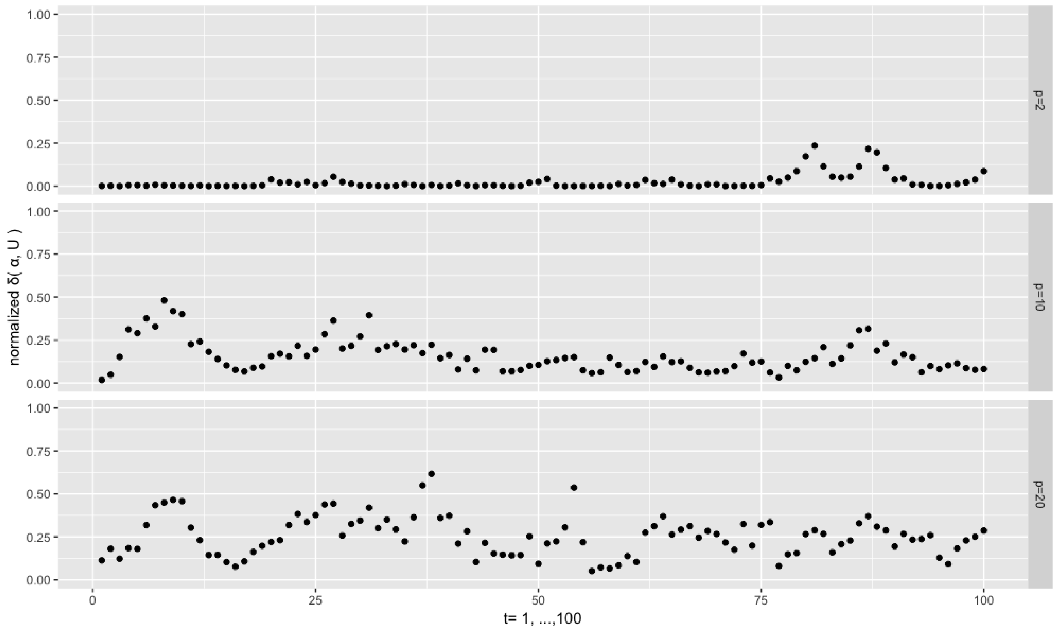
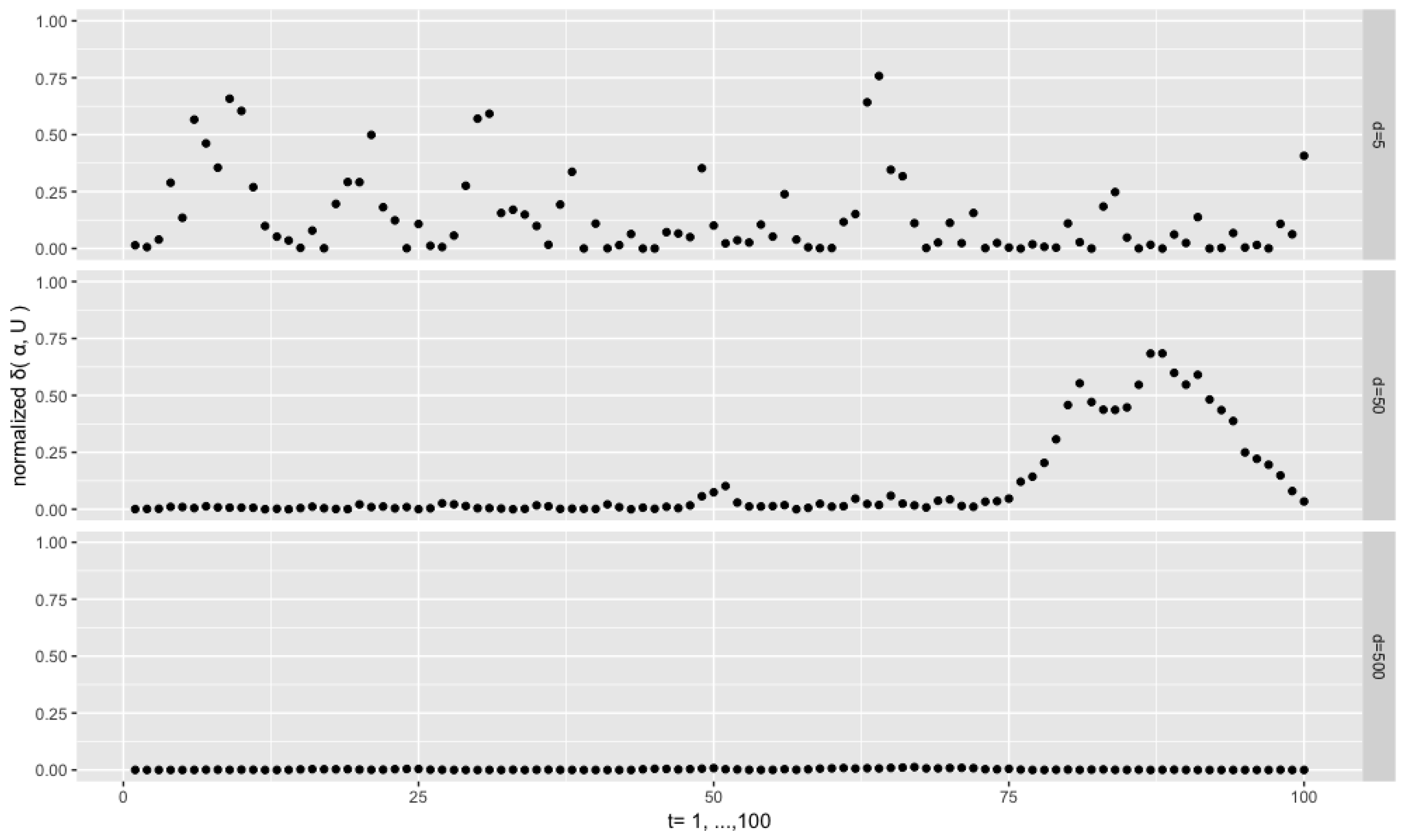
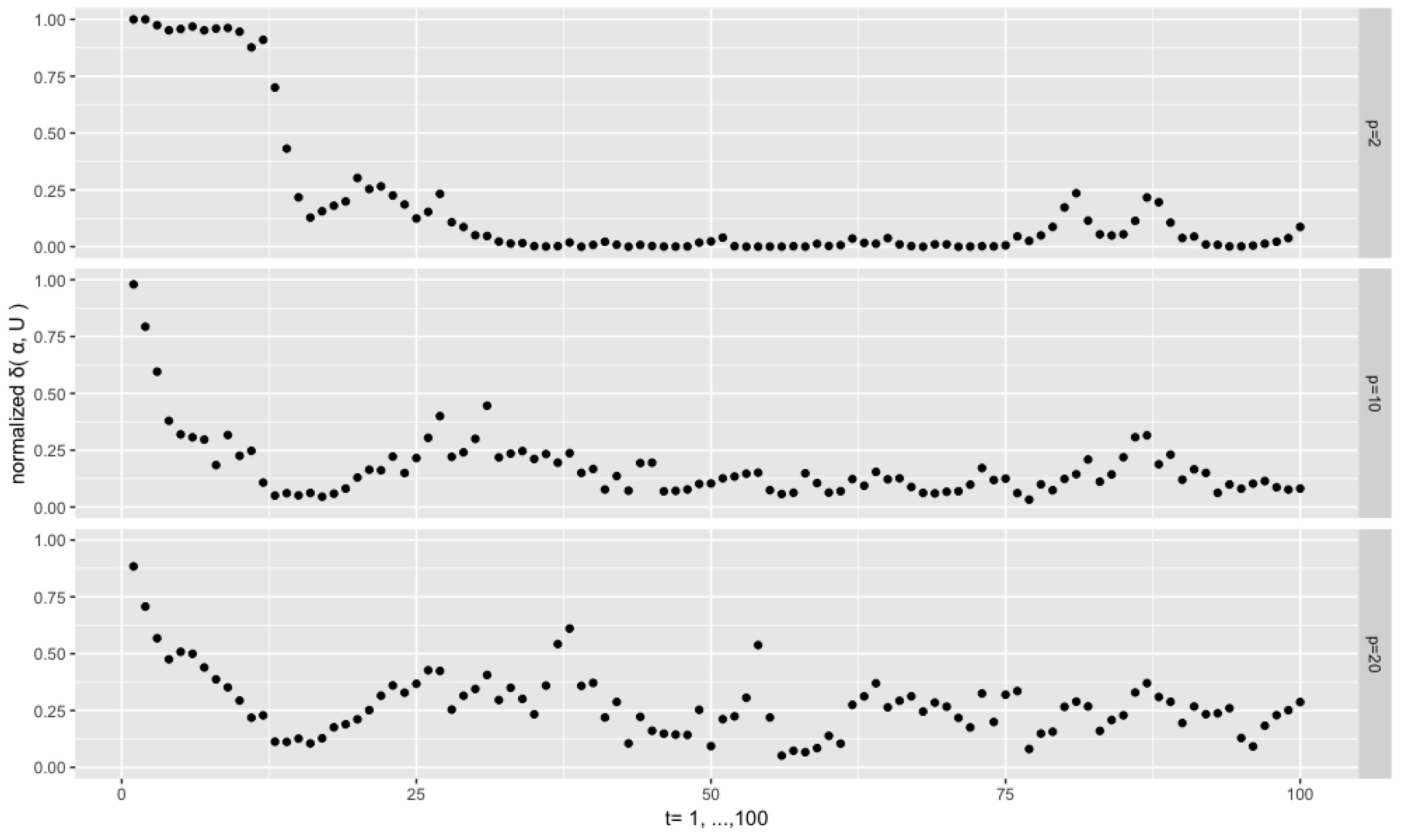
Figure 4 depicts the results from the setting $p\in \{2,10,20\}$, $r=1$, $\rho =0.1$ and $d=50$. We see that the sequences of the normalized distances ${\delta }_t$ are persistent. This is a common phenomenon throughout the experiments, and, intuitively, it can be attributed to the fact that the current ${\delta }_t$ depends on the previous one through the pair of ${\mathit{U}}_t$ and ${\mathbf{\alpha }}_t$. For the low dimensional case $p=2$, almost all the distances are very close to 0, which means that the filtered modal orientations are very close to the true ones, despite few exceptions. However, for the higher dimensional cases $p=10$ and 20, the distances are at higher levels and are more dispersed. This is consistent with the fact that, given the same concentration $d=50$, an increase of the dimension the orthonormal matrix or vector goes along with an increase of the dispersion of the corresponding distributions on the Stiefel manifold, as the volume of the manifold explodes with the increase of the dimensions (both p and r).

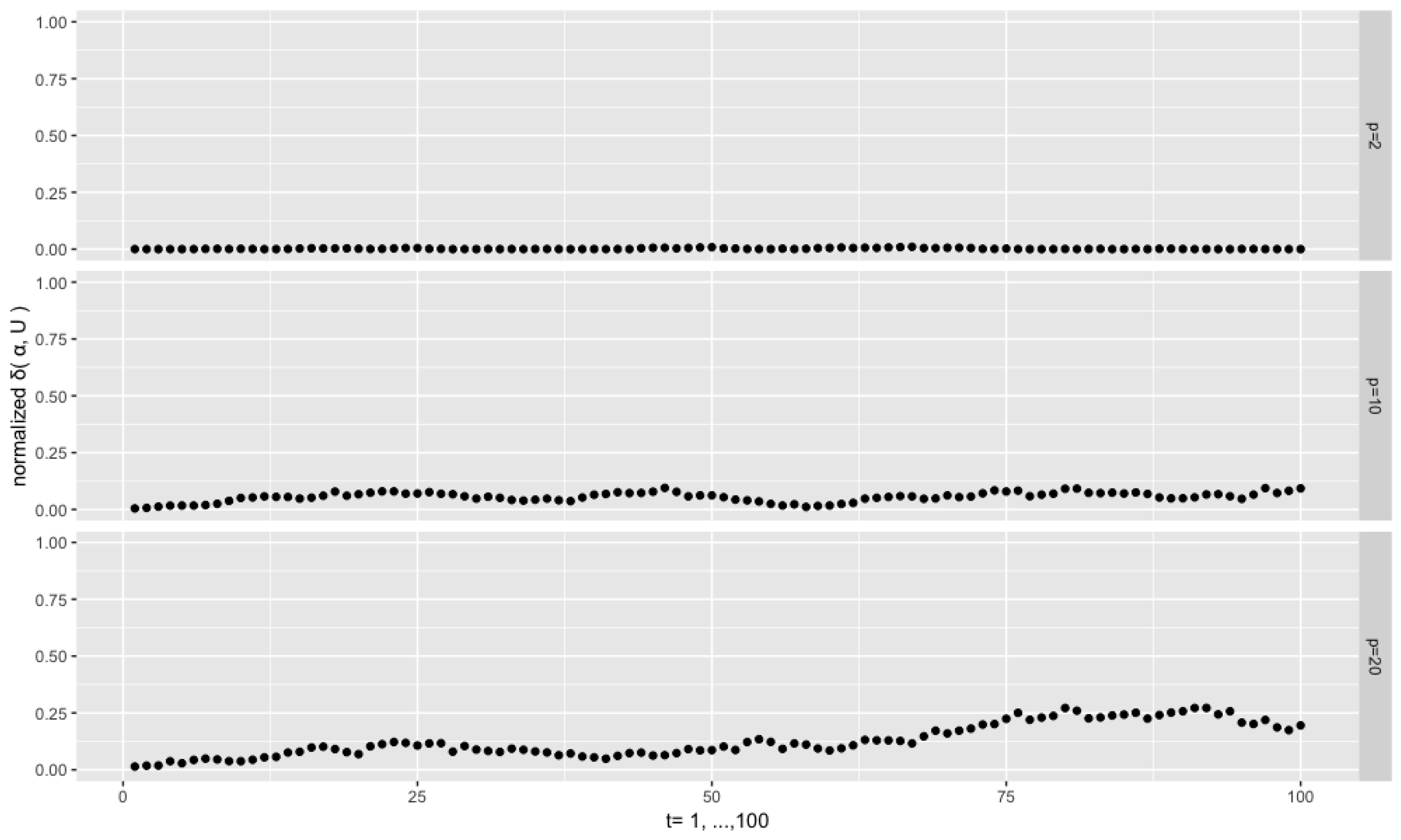
Figure 5 displays the results for the same setting $p\in \{2,10,20\}$, $r=1$, $\rho =0.1$ but with a much higher concentration $d=500$. We see that the curse of dimensionality can be remedied through a higher concentration as the distances for the high dimensional cases are much closer to zero than when $d=50$.

The magnitude $\rho$ of the variance of the errors affects the results of the filtering algorithm as well, as it determines the concentration of the filtering distribution, which can be seen from (39) through $\mathit{J}$ and ${\mathit{C}}_t$ (both depend on the inverse of $\mathsf{\Omega }$). The following experiments apply the settings $p=2$, $r=1$ and $d\in \{5,50,500\}$ showing the impact of different $\rho$ on the filtering results. Figure 6 depicts the results with $\rho =1$, and Figure 7 with $\rho =0.1$. We see that the normalized distances become closer to zero when a lower $\rho$ is applied. Their variability also decreases for the lowest value of $d=5$ and for the intermediate value $d=50$. It is worth mentioning that, in the two cases corresponding to the two bottom plots of the figures, the matrix ${\mathit{C}}_t$ dominates the density function, which implies that the filtering distribution resembles a highly concentrated matrix Langevin.

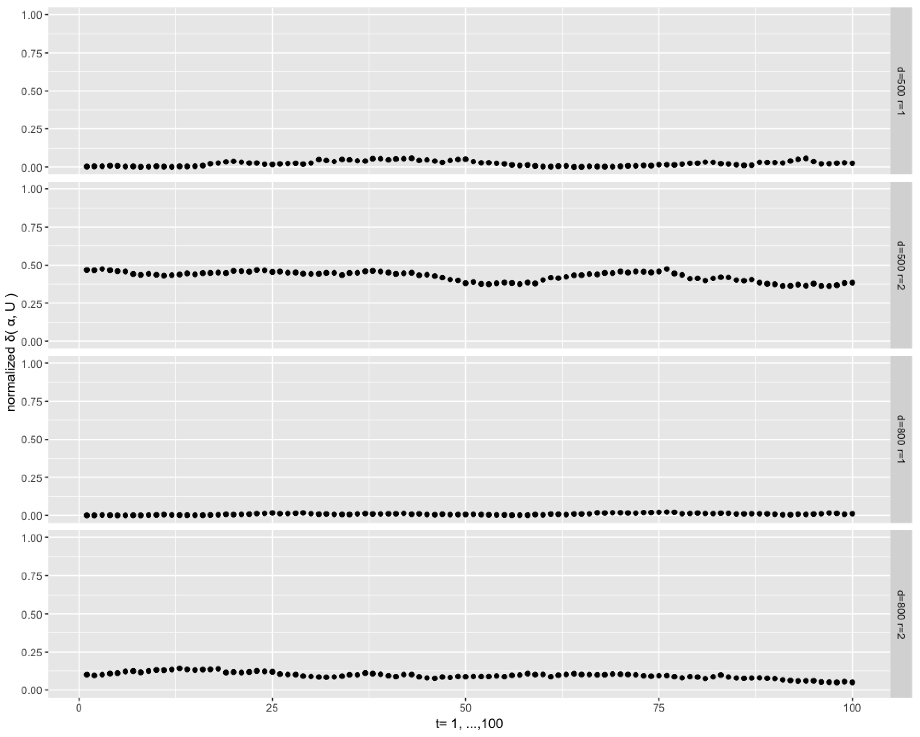
In the following experiments, our focus is on the investigation of the filtering algorithm when r approaches p. We consider the setting $p=3$ with the rank number $r\in \{1,2\}$, with $\rho =0.1$ and $d=500$. Figure 8 depicts the results. The normalized distances are stable at a low level for the case $p=3$ with $r=1$, but a high level (around 0.5) in the case $p=3$ with $r=2$. A higher concentration ($d=800$) reduces the latter level to about 0.12, as can be seen on the lower plot of Figure 8. We conclude that the approximation of the true filtering distribution tends to fail when the matrix ${\mathbf{\alpha }}_t$ tends to a square matrix, that is, $p\approx r$, and therefore the filtering algorithms proposed in this paper seems to be appropriate when p is sufficiently larger than r.

All the previous experiments are based on the true initial value ${\mathbf{\alpha }}_0$, but, in practice, this is unknown. The filtering algorithm may be sensitive to the choice of the initial value. In the following experiments, we look into the effect of a wrong initial value. The setting is $p\in \{2,10,20\}$, $r=1$, $\rho =0.1$ and $d=50$, and we use as initial value $-{\mathbf{\alpha }}_0$, which is the furthest point in the Stiefel manifold away from the true one. Figure 9 depicts the results. We see that in all the experiments the normalized distances move towards zero, hence the filtered values approach the true values in no more than 20 steps. After that, the level and dispersion of the distance series are similar to what they are in Figure 4 where the true initial value is used. Thus, we can conclude that the effect of a wrongly chosen initial value is temporary.

We have conducted similar simulation experiments for Model 2 in (19) to investigate the performance of the algorithm proposed in Proposition 4. We find similar results to those for Model 1. All the experiments that we have conducted are replicable using the R code available at https://github.com/yukai-yang/SMFilter_Experiments, and the corresponding R package SMFilter implementing the filtering algorithms of this paper is available at the Comprehensive R Archive Network (CRAN).

7. Conclusions

In this paper, we discuss the modelling of the time dependence of the time-varying reduced rank parameters in multivariate time series models and develop novel state-space models whose latent states evolve on the Stiefel manifold. Almost all the existing models in the past literature only deal with the case where the evolution of the latent processes takes places on the Euclidean space, and we point out that this approach can be problematic. These problems motivate the development of the novel state-space models. The matrix Langevin distribution is proposed to specify the sequential evolution of the corresponding latent processes over the Stiefel manifold. Nonlinear filtering algorithms for the new models are designed, wherein the integral for computing the predictive step is approximated by applying the Laplace method. An advantage of the matrix Langevin distribution is that the a priori and a posteriori distributions of the latent variables are conjugate. The new models can be useful when the temporal instability of some parameters of multvariate models is suspected, for example, cointegration models with time-varying short-run adjustment or time-varying long-run relations, and factor models with time-varying factor loading.

Further research is needed in several directions. The most obvious one is the implementation of estimation methods, which can be maximum likelihood or Bayesian inference, and the investigation of their properties. This will enable us to apply the models to data. In this paper, we only consider the case where the latent variables evolve on the Stiefel manifold in a ‘random walk’ way. It will be interesting to consider the case where the latent variables evolve on the Stiefel manifold but in a mean-reverting way.