Article

Financial Big Data Solutions for State Space Panel Regression in Interest Rate Dynamics

by
Dorota Toczydlowska
1,* and
Gareth W. Peters
2,1,3,4
1
Department of Statistical Science, University College London, 1-19 Torrington Place, London WC1E 7HB, UK
2
Department of Actuarial Mathematics and Statistics, Heriot-Watt University, Colin Maclaurin Building, Heriot-Watt University, Edinburgh EH14 4AS, UK
3
Man Institute of Quantitative Finance, University of Oxford, Oxford OX1 3BD, UK
4
Systemic Risk Center, The London School of Economics and Political Science, Houghton Street, London WC2A 2AE, UK
*
Author to whom correspondence should be addressed.
Econometrics 2018, 6(3), 34; https://doi.org/10.3390/econometrics6030034
Submission received: 12 February 2018 / Revised: 19 June 2018 / Accepted: 7 July 2018 / Published: 18 July 2018
(This article belongs to the Special Issue Big Data in Economics and Finance)

Abstract

:
A novel class of dimension reduction methods is combined with a stochastic multi-factor panel regression-based state-space model in order to model the dynamics of yield curves whilst incorporating regression factors. This is achieved via Probabilistic Principal Component Analysis (PPCA) in which new statistically-robust variants are derived also treating missing data. We embed the rank reduced feature extractions into a stochastic representation for state-space models for yield curve dynamics and compare the results to classical multi-factor dynamic Nelson–Siegel state-space models. This leads to important new representations of yield curve models that can be practically important for addressing questions of financial stress testing and monetary policy interventions, which can incorporate efficiently financial big data. We illustrate our results on various financial and macroeconomic datasets from the Euro Zone and international market.

1. Introduction

The increased collection and accessibility to complex financial and macroeconomic data are transforming the way in which financial services operate. Therefore, the methods that study such data for financial applications should acknowledge this progress in methodological developments and utilise increasingly big financial datasets to understand and reinterpret key financial applications such as interest rate dynamics. Furthermore, the increasing volume of market data poses both an opportunity and a challenge for financial institutions to deepen their understanding of market-wide and country-specific sources of risk present in financial markets and their implications for modelling and forecasting markets’ dynamics. Such information is of key importance for efficient investment decision making, understanding the influence of unconventional monetary policies and risk management procedures such as stress testing.
In this paper, we focus on providing a coherent methodology that utilises global macroeconomic and financial market datasets in modelling one of the most popular indicators of economic activity, the London Interbank Offered Rate (Libor). Libors are broadly used as benchmark rates for a wide collection of financial products. In order to use the information available in a range of financial datasets in a meaningful and parsimonious way to help explain the dynamics of Libor, we apply the feature extraction methodology with special tailoring for handling irregular time series (missing data) and outliers.

1.1. Multifactor Models for Yield Curve Dynamics

Before the financial crisis of 2007–2008, it was widely believed that interest rate dynamics were well specified by single interest rate models such as short-rate models, rational pricing kernels, forward single rate models (Heath–Jarrow–Morton or Libor market models) with a leading assumption that there were no arbitrage relations between the instruments associated with different tenors, and hence, the rates were feasibly modelled separately. The financial crisis changed this perception, uncovering not only the significant spreads between the rates of different tenors, which are no longer negligible, but also the arising discrepancies between the rates, which were very close before the crisis, such as Libor rates and Overnight-Index swaps. This resulted in the emergence of multi-curve interest rate models, which aim to capture the simultaneous presence of various interest rates and to reflect the implications of liquidity and credit risks resulting from lending in the interbank money market. For a discussion on the theory of interest models and the post-crisis challenges, the reader may refer to Grbac and Runggaldier (2015) or Cuchiero et al. (2016b). The study of Filipovic and Trolle (2013) discusses multiple factors, which are not captured by single rate models, but are proven to have a significant impact on the term structure of Libor. The authors indicated the influence of the default risk, which increases with a rate’s maturity and is a dominant driver of long maturities. The study highlights the importance of modelling the term structure of Libor rates.
The existing literature on modelling the term structure of interest rates can be divided into two sets. The first group of methodologies aims to perform the exact replication of observed market rates via stochastic interpolations. These models are useful for daily calibration on the term structure, but they are often not consistent on intraday dynamics. These term structure models are used in pricing or hedging applications. For details of methodological developments in the first class of models, the reader may refer to the recent studies of Chib and Ergashev (2009), Cuchiero et al. (2016b) or Cuchiero et al. (2016a) and notably the consistent prediction framework of Teichmann and Wuthrich (2016). The second class of approaches performs regression as opposed to interpolation. Such methods produce models more applicable to risk management, monetary policy and econometrics application such as stress testing, as they can be used as consistent in-sample estimations and forecasting applications.
The present study belongs to the second group of methods. We aim to develop under a regression state-space setting the incorporation of features extracted from macroeconomic and financial information present in big datasets, which explain the Euro Libor yield curve over time and are not associated with traditional yield curve factors. The current literature on incorporating macroeconomic and financial big data into financial modelling mostly focuses on the prediction of portfolio returns. The reader may refer to the well-known works of Cao and Tay (2003), Armano et al. (2005) or Kwon and Moon (2007) or the more recent studies of Geva and Zahavi (2014) and Kercheval and Zhang (2015) and Sirignano (2016) and Borovykh et al. (2017) for applications of advanced learning algorithms in finance. These approaches have one significant disadvantage: they leave the interpretation of the results behind without addressing the question of the individual influence of financial and macroeconomic features. Therefore, they are not applicable for policy making and stress testing purposes when one wants to source the information on interactions between market components.
The existing literature on incorporating market-specific information into yield curve modelling mostly focuses on using raw macroeconomic time series as exogenous, explanatory variables and incorporating them into a yield curve model by tracking the dynamics of their contributions to yield curve calibration over time. Other methods use compressed information obtained using feature extraction techniques from financial data. For instance, the authors of Diebold and Li (2006) used various economy condition proxies in addition to the components of the Nelson–Siegel model, introduced by Nelson and Siegel (1987), to show their significant link to U.S. Treasury yield and improve the forecast of the yield. The interactions between U.K. government bond yields and inflation, monetary rates and unemployment related proxies were combined in a stochastic volatility Nelson–Siegel model setting in Bianchi et al. (2009). Particular attention is focused on the contribution to the yield curve volatility under monetary policy shocks that introduces developments of a coherent stress testing methodology. The study of Joslin et al. (2014) further confirmed the substantial effects of inflation and economic activity on the U.S. Treasury yield curve by introducing the affine, arbitrage-free methodology, which incorporates the relevant macroeconomic factors. The approach to model simultaneously yield curve and filter unobserved macroeconomic variables using macroeconomic factors not spanned by classic yield curve components of the Nelson–Siegel model class is discussed in Coroneo et al. (2016), where the authors applied a dynamic factor methodology to the U.S. Treasury yields. More recently, Karimalis et al. (2017) proposed a multiple-country stress testing framework to efficiently capture the effects on the set of European government yield curves from shocks in country-specific liquidity and credit-related variables by employing two procedures: modelling of the dynamics of country-specific yield curves by employing the dynamic macro-finance Nelson–Siegel model of Diebold and Li (2006) and a robust covariance regression model applied to yield curves, both with the inclusion of macro-finance factors.

1.2. Feature Extraction Methods for Financial Data

The modelling of the yield curve in the presence of a data-rich environment requires an application of feature extraction methodologies in order to reduce the required model parameters and focus only on the incorporation of meaningful information into the model. A common practice in yield curve modelling is to use principal component analysis in order to reduce the dimensionality of the data and obtain features that explain the highest portion of the variance. Beginning with the study of Ang and Piazzesi (2003) or Emanuel Moench (2008), the authors used reduced information from inflation-linked and real economic activity-linked sets of U.S. financial markets by extracting the first principal component from each group of datasets and then adopting the Factor-Augmented Vector Autoregressive (FAVAR) model to calibrate the U.S. Treasury yield. The factor-augmented regression with static factors obtained by principal component analysis was introduced in Ludvigson and Ng (2010) to study the relation between bond excess returns and the macroeconomy. The use of international sovereign yield curves from leading economies in modelling, so-called, global yield curves, the sets of rates from leading countries, was investigated in Abbritti et al. (2013). The authors utilised the FAVAR framework to combine traditional determinants of the yield curve level, slope and curvature and three global factors. The other applications of incorporating features extracted from the sets of international sovereign yield curves in a term structure calibration are the work of Joslin et al. (2010), for the U.S. Treasury bond yields, or the study Wright (2011) that investigated the decomposition of the forward rates into expected future short-term interest rates and term premiums.
Hence, the following study contributes to the latter group of works in combining the financial market data feature extraction and modelling of the structure of yield curves. However, the novelty is largely in the attention to the efficient and statistically-robust feature extraction methodologies. We use international macroeconomic and financial big datasets to study the effects of global economies on the dynamics of the EUR Libor market. In order to handle the presence of irregularities in the real data time series and the possibility of outliers, we develop a novel statistically-robust class of methods for feature extraction based on probabilistic principal component analysis introduced by Tipping and Bishop (1999). Our extension uses reference distributions based on two versions of the multivariate t-Student. The extracted features are used as predictors and are incorporated into a novel dynamic state-space formulation of Nelson–Siegel model of Nelson and Siegel (1987) following the work of Diebold and Li (2006), with application to the EUR Libor yield curve.
Principal Component Analysis (PCA) and related matrix factorisation methodologies are widely used in data-rich environments as dimensionality reduction, data compression or feature extraction techniques. The methodologies identify a lower dimensional subspace to represent the data, which captures second order dominant information contained in the data. The general matrix representation of the problem assumes that the observation data matrix can be decomposed into the sum of a lower-rank matrix and a matrix of observation noise. In practice, we may identify the four most straightforward distant patterns of possible noise matrices, which are exemplified in Zhou et al. (2010). According to their abundance and the magnitude of their values, the noise matrices may have sparse or dense noise values and small or large values. Since standard PCA assumes a quadratic loss function, it is only efficient in the cases of small and dense noise. Due to this fact, the methodology is highly sensitive to distant data points, called outliers, which corrupt the sample set. In order to improve the robustness of PCA, there have been many extensions to the standard methodology proposed. The most straightforward approach is to improve the estimation of the sample moments in the PCA procedure by using their robust alternatives as in Hubert et al. (2005). The concept of robust estimators has been further extended in Huber (1964), Rousseeuw and Yohai (1984), Rousseeuw (1985) and Tyler (1987) and is broadly discussed in the existing literature in the context of robust methods for principal component analysis as in Maronna (2005) or Huber and Ronchetti (2009).
The other studies improve PCA by replacing the standard quadratic error function by some more robust alternatives, which weight the squared loss of each observation. The study De la Torre and Black (2001) investigates an M-estimation weighting algorithm for a minimisation of the error function. Another approach is based on using a loss function, which resembles the assumption on the heavy tail distribution of the data according to a Laplace Ke and Kanade (2005), Ding et al. (2006), Eriksson and Hengel (2012) or Cauchy Xie and Xing (2015) type of error function. The Laplace loss function is very convenient to work with datasets that exhibit large, sparse noises, as the L 1 norm forces sparsity of the solution, as shown in Tibshirani (1996). When working with larger and dense noises, it is more convenient to use the Cauchy type of loss function. The authors of Candes et al. (2009) or Zhou et al. (2010) proposed stable principal component pursuit, a methodology that combines both of these noise patterns. They investigate the model for PCA, which decomposes the data into the lower rank, small and dense noise matrices and a large and sparse noise matrix.
However, the non-probabilistic frameworks are difficult when one wants to specify various a priori assumptions about the distribution of the observation process in order to achieve some desirable probabilistic model properties, which are especially efficient in handling the presence of missing data or incomplete observations. The probabilistic paradigm of standard PCA has been introduced by Tipping and Bishop (1999) as Probabilistic Principal Component Analysis (PPCA), where the noise vector is assumed to follow a Gaussian distribution. In order to robustify the framework, the studies Khan and Dellaert (2003), Archambeau et al. (2006), Fang and Jeong (2008) and Chen et al. (2009) suggested to use an independent in time t-Student assumption on the noise distribution. Deriving the PPCA results then follows by remarking that t-Student is an infinite mixture of Gaussian random variables. To improve the resistance of PPCA to large, sparse noises, the authors of Ke and Kanade (2005) and Eriksson and Hengel (2012) replaced the Gaussian distribution with the Laplace distribution. All of these methodologies assumed latent vectors and the error terms to be mutually independently distributed variables with the same degrees of freedom denoted by v and independent over time with different probability functions over time, and they can be perceived as independent variables, which is not always the case in practice.
In the following study, we extend the PPCA models by forcing all observations to be distributed identically and, hence, examining the elements of the sample set as the realisations of one random variable in time. We derive and examine the proposed methodology for the t-Student distribution, which is a heavy-tailed alternative to the Gaussian distribution and is suitable to work with financial and macroeconomic data that are corrupted by dense gross errors.

1.3. Contributions and Structure

The manuscript can be split into two main parts corresponding to our two main contributions to feature extraction and dynamic yield curve modelling.
Our first contribution is a novel identical and conditional t-Student PPCA methodology and its estimation framework, which allows for efficient statistical estimation in the presence of missing data. In the first part of this manuscript, we show how to compress the information available in the big datasets in a meaningful manner. We discuss extensions of the probabilistic approach to feature extraction based on the widely-adopted principal component analysis. We assume that the multivariate observation vector follows a t-Student distribution in order to tackle the possibility of distant data points, distinguishing between two cases: when the observations are independent over time or identically distributed. The developed methodology ensures robustness by allowing various prior assumptions on the heaviness of tails of the examined data. In addition, the probabilistic methodology efficiently handles the missing values of the time series in big datasets. We illustrate how to use this framework for econometric studies on financial big datasets.
Our second contribution is extending the state space structure of the Nelson–Siegel yield curve model to efficiently incorporate additional factors. We discuss the methodology of incorporating meaningful market information into an econometric model of a yield curve. We show how to extend the model, which calibrates and forecasts the Euro Libor yield curve in order to utilize available market information. Such a model can serve as a useful tool for a parsimonious stress testing exercise. The introduction of the methodology is followed by the discussion of an optimal estimation technique based on the Kalman filter studied by Kalman and Bucy (1961). We perform comprehensive state-space model selection and structuring, and the in-sample and out-of-sample analysis confirms that our methodology outperforms the standard method.
The utilisation of the market information in yield curve modelling is well documented in the current literature. In the study of Diebold and Li (2006), the authors extended the dynamic Nelson–Siegel model of Nelson and Siegel (1987) by including observable macroeconomic variables in order to investigate the interaction between the macroeconomy and a yield curve. Nevertheless, given the current availability of the data, we find this approach disadvantageous due to two aforementioned reasons: the high possibility of the model over parametrization and hidden links between various datasets that may spoil the modelling quality. Therefore, instead of incorporating raw data, we discuss how to use the derived market features.
The paper is organised as follows. The list of datasets used in this study is detailed in Section 2. The novel extensions to the probabilistic principal component analysis are discussed in Section 3, whereas the steps of the employed estimation procedure, the expectation-maximisation algorithm, is derived in Section 4. The detailed proofs of the steps of derivations are provided in the Appendix which can be accessed online as Supplementary Material. Section 5 introduces the concept of yield curve modelling, as well as extends the framework by showing how to incorporate the market-specific features in an econometric manner. The subsequent parts of the section overview the employed methodology of the model estimation and selection. The outcomes of the derived methodologies of feature extraction applied to real datasets are discussed in Section 6. The framework for the calibration and forecasting Euro Libor yield curve is examined on real data studies presented in Section 7. The last section concludes.

2. International Macroeconomic and Financial Big Datasets

In the following section, we briefly overview various international macroeconomic and financial datasets that are investigated in this study, summarized in Table 1. We advise the reader to refer to Appendix A in the Supplementary Material for a detailed discussion and insight into the investigated time series.
Our attention is focused on investigating features that measure Euro Zone market conditions and their decomposition into their influences from the domestic and international markets. The Euro Zone market is represented by the Euro Libor yield curve. We collect the data from leading domestic and global economies, in total 12 countries, categorized as follows:
Domestic economies: 
Germany (DE), France (FR), Portugal (PO), Spain (ES), Italy (IT), Ireland (IR) and the United Kingdom (GB);
International economies: 
Japan (JP), United States (U.S.), Australia (AU), Brazil (BR) and South Africa (SA).
The subsets of data that serve to investigate various domestic and global influences are categorized as follows:
GOV: 
the panel valued time series, which measure the interactions between country-specific sovereign yield curves;
INF: 
the panel valued time series, which measures the influence of country-specific inflation risks represented by inflation-linked yield curves and Consumer Price Indexes;
PRD: 
the time series that measures the influence of country-specific productivity proxies represented by Gross Domestic Product (GDP), unemployment rates and Labour productivity;
FX: 
the time series that measures the interactions between leading foreign exchange markets and the Euro Zone market given by exchange rates for the Euro (EUR) and Japanese Yen (JPY), United States dollar (USD) and Australian dollar (AUD);
LIQ: 
the time series that serves as a proxy of Euro Zone liquidity represented by 3M Euro Repo and Euribor rates and German Bund Open Interest;
CR: 
the time series that are used as proxies of the credit quality of the Euro Zone given by the 5YMarkit Intraxx Index.
The instruments described by the three first rows of Table 1 are country-specific yield curves, which have a term structure. Therefore, their one observation is a multidimensional vector with elements corresponding to the rates with specific maturities belonging to the set τ 1 months ( M ) , 3 months ( M ) , , 20 years ( Y ) .

3. Novel Feature Extraction via Probabilistic Principal Component Methods Using the t-Student Formulation

In the following part, we discuss the existing PPCA methodologies, as well as provide our novel model extending the standard methods in the presence of missing data in an efficient and statistically-robust manner.
We discuss the feature extraction methodologies that adapt principle component analysis to a probabilistic formulation in order to reduce the dimensionality in the presence of data that contain realistic features such as missingness, as well as outliers and noise. Such techniques should be applicable to very large time series datasets.
We choose to focus on robust alternatives to the Gaussian PPCA, and we demonstrate how to use the t-Student distribution in order to account for heavy tail assumptions, which result in the methodology being statistically robust to the distant observations in a sample set of outliers. We investigate two t-Student frameworks, one in which the observations are assumed to be independent over time, which leads to different probability density functions over time, and the second in which the observation vectors are assumed to be identically distributed and conditionally independent over time. The first concept had been partially introduced by Lange et al. (1989), whereas the latter is our novel contribution to the existing literature on the probabilistic principal component analysis. The extended frameworks of the derived methodologies provides the consistent statistical incorporation of missingness.

3.1. Introduction to Probabilistic Principal Component Analysis

Let us define the random vector with observations in time t, Y t R d and the random vector of latent (unobserved) variables X t R k for d , k N . The relation between the observed values Y t and the hidden variable, X t is defined by the following model:
Y t = μ + X t W d × k T + ϵ t
for ϵ t being a d-dimensional error term with covariance matrix σ 2 I d , W a real valued d × k matrix and μ a d-dimensional intercept vector.
The existing literature introduces the concept of using the t-Student distribution to achieve this purpose. The reader may refer to Lange et al. (1989), Archambeau et al. (2006), Fang and Jeong (2008) or Chen et al. (2009) where the latent vectors and the error terms are mutually independently distributed t-Student variables with the same degrees of freedom denoted by v and independent over time. In addition, the authors assume the vectors of the response variable, Y t , to be independent over time, which forces each of the observations to be treated as an individual random variable with different probability functions. This assumption also requires X t and ϵ t to have different probability distributions over time. The assumptions provide the PPCA framework with the flexibility to treat each of the observations individually; however, this adds additional degrees of freedoms to an estimation problem, which may cause unnecessary difficulties when the sample size is not sufficiently large. Further, the statistical characteristic of the observation set, as well as the latent processes over time are limited since every realisation of the variables over time is distributed separately.
As a possible remedy to the listed limitations of Independent t-Student PPCA (t-Student IND PPCA), we propose an extension to the methodology by assuming X t and ϵ t to be identically distributed, that is the observations have the same probability distribution over time and therefore are treated as realisations of one random variable. The reader will see that the assumption of the identical distribution preserves the mutual independence of X t and ϵ t , but restricts them to be only conditionally independent over time. In addition, we add a second important extension not previously explored in this literature, which allows dealing with the general missingness structures in the response vectors Y t over time.

3.2. t-Student Principal Component Analysis

Let us denote Ψ as a vector of all static parameters of model (1), that is Ψ = [ W , μ , σ 2 , v ] . Consider the definition of the t-Student random variable density (see Gupta and Nagar 1999) rewritten as a mixture of Gaussian and Gamma random variables. One may then define the sequence of scalar Gamma random variables U t Γ ( v 2 , v 2 ) for t = 1 , N , whose elements are independent over time. The stochastic representations of t-Student random vectors X t and ϵ t may then be expressed by:
X t = 1 U t Z x , t , ϵ t = σ 2 U t Z ϵ , t ,
where Z ϵ , t and Z x , t are mutually independent d and k-dimensional standard normal random vectors, respectively, which are independent over time. The joint probability functions of model (1) in the independent t-Student case, for N realisations of Y t , is then given by:
π Y 1 : N , X 1 : N , U 1 : N | Ψ y 1 : N , x 1 : N , u 1 : N = t = 1 N π Y t | X t , U t , Ψ ( y t ) π X t | U t , Ψ ( x t ) π U t | Ψ ( u t ) ,
where the conditional distributions of Y t | X t , U t , Ψ and X t | U t , Ψ are Gaussian such that:
Y t | X t , U t , Ψ N μ + X t W T , σ 2 U t I d   and   X t | U t , Ψ N 0 , 1 U t I k .
We extend the concept of t-Student IND PPCA by proposing a more parsimonious model requiring a reduction of integrals from N to 1 when marginalizing to get the distribution of Y 1 : N . The latent variable U is no longer time dependent, and the methodology assumes one realisation of U Γ v 2 , v 2 for the sample set. Consequently, the variables X t and ϵ t are identically distributed. The stochastic representations of X t and ϵ t under the identical and conditionally independent t-Student distributed model is given by:
X t = 1 U Z x , t , ϵ t = σ 2 U Z ϵ , t .
The vectors X t and ϵ t are independent over time only when conditioned on U. Under these assumptions, the observation vector Y t is still conditionally multivariate Gaussian:
Y t | X t , U , Ψ N μ + X t W T , σ 2 U I d ,
but is not marginally independent over time, which results in the following joint probability density function of the model (1) in the identical and conditionally independent t-Student PPCA (t-Student IID PPCA) case:
π Y 1 : N , X 1 : N , U | Ψ ( y 1 : N , x 1 : N , u ) = π Y 1 : N | X 1 : N , U , Ψ ( y 1 : N ) · π X 1 : N | U , Ψ ( x 1 : N ) · π U | Ψ ( u ) = π U | Ψ ( u ) t = 1 N π Y t | X t , U Ψ ( y t ) · π X t | U , Ψ ( x t ) .

3.3. Novel Extension of Probabilistic Principal Component Analysis for a Missing Data Setting

The probabilistic principal component analysis is especially efficient in the presence of missing data. In the following, we show how to model the incompleteness of the observations in a PPCA framework.
To achieve this, the vector Y t is partitioned into two subvectors, one that contains observed values Y t o and the second that indicates missing entries Y t m , such that Y t = Y t o , Y t m . We denote d o as the number of observed elements of the vector Y t and d m = d d o the number of missing entries in time t.
Let us define an indicator random variable R t { 0 , 1 } d that decides which entries of Y t are missing, one indicating not missing and zero otherwise. In the incomplete data setting, a single observation consists of the pair Y t o , R t with some distribution parameters Ψ , Ψ r , respectively. We assume the parameters to be distinct. The likelihood of the parameters is proportional to the conditional probability Y t o , R t | Ψ , Ψ r , given by:
π Y t o , R t | Ψ , Ψ r ( y t o , r t ) = π Y t o , Y t m , R t | Ψ , Ψ r ( y t o , y t m , r t ) d y t m = π R t | Y t , Ψ , Ψ r ( r t ) · π Y t | Ψ , Ψ r ( y t ) d y t m .
In this study, we assume a Missing-At-Random (MAR) statistical framework, as defined in Little and Rubin (2002). This restricts the missingness to appear independently of the magnitude of the unobserved values. Given this assumption, we will demonstrate in the following (see further details in Section 4) how this result will be critical in an expectation maximisation algorithm. We will demonstrate importantly that under such a framework, the required expectations do not account for the distribution of the indicator variable since the vector Y t under MAR satisfies:
π R t | Y t , Ψ r ( r t ) = π R t | Y t o , Ψ r ( r t ) .
resulting in:
π Y t o , R t | Ψ , Ψ r ( y t o , r t ) = π R t | Y t o , Ψ r ( r t ) π Y t | Ψ ( y t ) d y t m = π R t | Y t o , Ψ r ( r t ) · π Y t o | Ψ ( y t o ) .
Under the MAR assumption, the estimation of Ψ via the maximum likelihood of the joint distribution Y t o , R t | Ψ , Ψ r is equivalent to the maximisation of the likelihood of the marginal distribution Y t o | Ψ . Hence, we are not concerned about the distribution of the indicator random variable R t and the distribution of Y t o and R t . If the assumption about MAR does not hold, one needs to solve the integral from Equation (6) in order to maximize the joint likelihood.
In the incomplete data case-related sections, we denote by W o and W m the d o × k and d m × k non-squared submatrices of W with corresponding rows to the elements of the vector Y t , which are observed and missing, respectively. In general, by lower index o and m, we further refer to the elements of some objects corresponding to observed and missing values of Y t , respectively.

4. EM Algorithm for the Probabilistic Principal Component with t-Student Distribution

In order to develop a procedure for estimating the static parameters and extracting the filtered hidden variables, the factor loadings of the principal components from the model (1) under various assumptions specified in Section 3, we employ an Expectation-Maximisation (EM) Algorithm introduced by Dempster et al. (1977). The algorithm is particularly useful when we need to calculate the likelihood of incomplete data by integrating with respect to latent variables. It is efficiently achieved in two iterative steps, which jointly maximize the expected log-likelihood of the data, both observed and hidden variables. Given the models from the exponential family, this technique ensures that the local maximum of the incomplete data likelihood is reached. Given the presence of missing information, the two steps of the EM algorithm for the model (1) are given by:
Step 1:
Expectation step (E-step):
The expectation of the conditional distribution Y 1 : N m , X 1 : N | Y 1 : N o over the logarithm of the joint probability function of the observed and hidden variables of the model (1) given N realisations of the variables as a function of the two vectors with static parameters Ψ = [ W , μ , σ 2 ] and Ψ = [ W , μ , σ 2 ] , that is:
Q Ψ , Ψ = E Y 1 : N m , X 1 : N | Y 1 : N o , Ψ log π Y 1 : N , X 1 : N | ψ y 1 : N , x 1 : N
Step 2:
Maximisation step (M-step):
Re-estimation of the vector of static parameters Ψ is carried out via maximisation of the resulting function Q with respect to the vector Ψ :
Ψ ^ = argmax Ψ Q Ψ , Ψ
Recall that the vectors Ψ and Ψ are, respectively, an old and updated version of the static parameters.
In the following section, we derive novel closed-form solutions to evaluate each step of the EM algorithm for t-Student PPCA cases. We show how to incorporate prior assumptions about the presence of missing data in the model, and we derive a novel robust missing data EM algorithm, which adapts the t-Student distribution to handle the incomplete data case. Each of the versions of the algorithm is derived for the two PPCA cases described in Section 3. The proofs of the theorems from the section are explained in Appendix D in the Supplementary Material.
The EM algorithm for t-Student variants of PPCA is used to estimate the parameters W , μ , σ 2 and the filtered values of unobserved processes. Recall that the models introduced in Section 3 depend on one additional parameter, v, corresponding to the degrees of freedom, which determine the t-Student probability function. We will show in Appendix E in the Supplementary Material that the likelihood profile of the EM algorithms for the two variances of t-Student PPCA is very flat over the grid of degrees of freedom, and we recommend against using the EM algorithm to specify v. Therefore, we employ an independent grid-based search to choose v by setting v and proceeding with EM algorithms for W , μ , σ 2 , which are derived in this section. The value of the scale parameter that obtains the highest log-likelihood is then chosen as an estimate of v.
As discussed in Section 3.3, We assume that random components of the observation process are unobservable, i.e., each observation of the process Y t can be partitioned into the two d o - and d m -dimensional subvectors Y t = [ Y t o , Y t m ] . The sample, which contains N realisations of the process Y t , is denoted by y 1 : N = y 1 , , y N , which can be partitioned into the subsamples y 1 : N = [ y 1 : N o , y 1 : N m ] , which contain observations of the subvectors Y t o and missing entries of Y t m for t = 1 , , N .

4.1. EM Algorithm for the Probabilistic Principal Component with the Independent t-Student Distribution in the Presence of Missing Data

The EM algorithm treats the vectors of missing observations Y t m as an additional hidden variable. Therefore, the E-step for the independent t-Student PPCA case with missingness needs to adjust for this latent process. The E-step is calculated as an expectation of the joint probability function from Equation (3) with respect to the conditional distribution Y 1 : N m , X 1 : N , U 1 : N | Y 1 : N , Ψ given the assumption in Equation (2). The expectation denoted as Q is given in Theorem 1. The maximizers of the function Q with respect to the vector of static parameters Ψ are specified in Theorem 2.
Theorem 1.
The E-step of the EM algorithm for t-Student IND PPCA given realisations of N observation vectors Y 1 : N o denoted by y 1 : N o = y 1 o , , y N o is given by:
Q ( Ψ , Ψ ) = E Y 1 : N m , X 1 : N , U 1 : N | Y 1 : N o , Ψ log π Y 1 : N , X 1 : N , U 1 : N | Ψ ( Y 1 : N , X 1 : N , U 1 : N ) = 1 2 t = 1 N [ d + k v 2 log 2 π + d log σ 2 + 1 σ 2 Tr E Y t m , U t | Y t o , Ψ U t Y t μ T Y t μ ( d + k + v 2 ) E U t | Y t o , Ψ log U t 2 σ 2 t r W E Y t m , X t , U t | Y t o , Ψ U t X t T Y t E Y t m , X t , U t | Y t o , Ψ U t X t T μ + t r 1 σ 2 W T W + I k E Y t m , X t , U t | Y t o , Ψ U t X t T X t + v E U t | Y t o , Ψ U t 2 log v 2 v 2 Γ v 2 ]
for the corresponding moments of the conditional distribution Y t m , X t , U t | Y t o , Ψ :
E U t | Y t o , Ψ U t = v + d o v + D t o , E U t | Y t o , Ψ log U t = ψ v + d o 2 log v + D t o 2 , E Y t m | Y t o , U t Ψ Y t 1 × d = y t o μ m + y t o μ o W o W o T + σ 2 I d o 1 W o W m T , E Y t m , U t | Y t o , Ψ U t Y t 1 × d = E U t | Y t o , Ψ U t E Y t m | Y t o , U t Ψ ( Y t ) , E Y t m , U t | Y t o , Ψ U t Y t T Y t d × d = 00 0 C m m W m W o T C o o 1 W o W m T + E U t | Y t o , Ψ U t E Y t m | Y t o , U t , Ψ Y t T E Y t m | Y t o , U t , Ψ Y t , E Y t m , X t , U t | Y t o , Ψ U t X t 1 × k = E U t | Y t o , Ψ U t E Y t m | Y t o , U t Ψ Y t W M 1 , E Y t m , X t , U t | Y t o , Ψ U t X t T X t k × k = σ 2 M 1 + M 1 W T E Y t m , U t | Y t o , Ψ U t Y t μ T Y t μ W M 1 , E Y t m , U t | Y t o , Ψ U t Y t μ T Y t μ = E Y t m , U t | Y t o , Ψ U t Y t T Y t 2 μ T E Y t m , U t | Y t o , Ψ U t Y t + E U t | Y t o , Ψ U t μ T μ , E Y t m , U t | Y t o , Ψ U t Y t T X t d × k = E Y t m , U t | Y t o , Ψ U t Y t T Y t E Y t m , U t | Y t o , Ψ U t Y t T μ W M 1 .
for C = W W T + σ 2 I d , M k × k = W T W + σ 2 I k , D t o ( y 1 : N o ; Ψ ) = y t o μ o C o o 1 y t o μ o T and ψ ( · ) the digamma function.
Proof. 
The proof of Theorem 1 is given in Appendix D.2.1. in the Supplementary Material. ☐
Theorem 2.
The maximizers of Q Ψ , Ψ are the solution to the set of equations given by Ψ Q = 0 . The maximizers with respect to μ , W   and   σ 2 can be obtained in closed-form according to the following solutions:
μ = 1 u ¯ ( y 1 : N o ; Ψ ) μ ¯ t s ( y 1 : N o ; Ψ ) I d W M 1 W T + u ¯ ( y 1 : N o ; Ψ ) μ W M 1 W T , W = C ¯ μ , μ t s ( y 1 : N o ; Ψ , Ψ ) W M 1 σ 2 M 1 + M 1 W T C ¯ μ t s ( y 1 : N o ; Ψ ) W M 1 1 , σ 2 = 1 d t r C ¯ μ t s ( y 1 : N o ; Ψ , Ψ ) 2 W M 1 W T C ¯ μ , μ t s ( y 1 : N o ; Ψ , Ψ ) + W T W σ 2 M 1 + M 1 W T C ¯ μ t s ( y 1 : N o ; Ψ ) W M 1
where:
u ¯ ( y 1 : N o ; Ψ ) = 1 N t = 1 N v + d o v + D t o , μ ¯ t s ( y 1 : N o ; Ψ ) = 1 N t = 1 N v + d o v + D t o E Y t m | Y t o , U t , Ψ Y t , S ¯ t s ( y 1 : N o ; Ψ ) = 1 N t = 1 N v + d o v + D t o ( y 1 : N o ; Ψ ) E Y t m | Y t o , U t , Ψ Y t T E Y t m | Y t o , U t , Ψ Y t , Q ¯ = 0 0 0 W m W m T + σ 2 I d m W m W o T W o W o T + σ 2 I d o 1 W o W m T , C ¯ μ t s ( y 1 : N o ; Ψ ) = S ¯ t s ( y 1 : N o ; Ψ ) + Q ¯ 2 μ T μ ¯ t s ( y 1 : N o ; Ψ ) + u ¯ ( y 1 : N o ; Ψ ) μ T μ , C ¯ μ t s ( y 1 : N o ; Ψ , Ψ ) = S ¯ t s ( y 1 : N o ; Ψ ) + Q ¯ 2 μ T μ ¯ t s ( y 1 : N o ; Ψ ) + u ¯ ( y 1 : N o ; Ψ ) μ T μ , C ¯ μ , μ t s ( y 1 : N o ; Ψ , Ψ ) = S ¯ t s ( y 1 : N o ; Ψ ) + Q ¯ μ + μ T μ ¯ t s ( y 1 : N o ; Ψ ) + u ¯ ( y 1 : N o ; Ψ , Ψ ) μ T μ ,
for M k × k = W T W + σ 2 I k , D t o ( y 1 : N o ; Ψ ) = y t o μ o C o o 1 y t o μ o T where C o o = W o W o T + σ 2 I d o .
Proof. 
The proof of Theorem 2 is given in Appendix D.2.2. in the Supplementary Material. ☐

4.2. EM Algorithm for the Probabilistic Principal Component with the Identical and Conditionally Independent t-Student Distribution in the Presence of Missing Data

Analogously to the previous subsection, we provide the E-Step and M-step for t-Student IID PPCA in Theorems 3 and 4. In this framework, we assume the identical probability model of X t and ϵ t ; however, now, we only assume a restricted conditional independence and identical distribution of the variables X t and ϵ t over time. This restriction we show still admits a closed-form solution.
Theorem 3.
The E-step of the EM algorithm for the t-Student IID PPCA given N realisations of the observation vector Y t o , denoted by y 1 : N o = y 1 o , , y N o , is given by:
Q ˜ ( Ψ , Ψ ) = E X 1 : N , Y 1 : N m , U | Y 1 : N o , Ψ log π Y 1 : N , X 1 : N , U | Ψ Y 1 : N , X 1 : N , U = C H ( Ψ ) C β ( y 1 : N o , Ψ ) π Y 1 : N o | Ψ ( y 1 : N o ) R + π ˜ U | Ψ ( u ) log π U | Ψ ( u ) d u + R + π ˜ U | Ψ ( u ) t = 1 N w ˜ ( y t o , u ; Ψ , Ψ ) d u
where the scalar C H is defined as in Lemma S4, the function w ˜ : R d o × N × R + R in Lemma S5 and the functions C β : R d o × N R and the density π ˜ U | Ψ ( u ) are derived in Lemma S6. Each of these ancillary lemmas and function definitions are contained in Appendix D.3.1. in the Supplementary Material.
Proof. 
The proof of Theorem 3 is contained in Appendix D.3.2. in the Supplementary Material. ☐
Theorem 4.
The maximizers of Q ˜ Ψ , Ψ are the solution to the set of equations Ψ Q ˜ = 0 . The maximizers with respect to μ , W and σ 2 can be obtained in closed-form according to the following solutions:
μ = μ ¯ ( y 1 : N o ; Ψ ) I d W M 1 W T + μ W M 1 W T , W = σ 2 Q ¯ + α β ( y 1 : N o ; Ψ ) C ¯ μ , μ ( y 1 : N o ; Ψ , Ψ ) W M 1 × M 1 W T σ 2 Q ¯ + α β ( y 1 : N o ; Ψ ) C ¯ μ ( y 1 : N o ; Ψ ) W M 1 + σ 2 M 1 1 , σ 2 = 1 d ( σ 2 Tr M 1 W T W + Tr σ 2 Q ¯ + α β ( y 1 : N o ; Ψ ) C ¯ μ ( y 1 : N o ; Ψ , Ψ ) 2 Tr σ 2 Q ¯ + α β ( y 1 : N o ; Ψ ) C ¯ μ , μ ( y 1 : N o ; Ψ , Ψ ) W M 1 W T + Tr M 1 W T σ 2 Q ¯ + α β ( y 1 : N o ; Ψ , Ψ ) C ¯ μ ( y 1 : N o ; Ψ ) W M 1 W T W
for the scalar α = v 2 + d o N 2 and the function β : R d o × N R :
β ( y 1 : N o ; Ψ ) = v 2 + 1 2 σ 2 t = 1 N y t o μ o V o o y t o μ o T .
defined as in Lemma 6 in Appendix D.3.1. in the Supplementary Material, the matrices V d × d = I d W M 1 W T and M k × k = W T W + σ 2 I k and the following function of y 1 : N o ,
E Y t m | Y t o , U , Ψ Y t = y t o μ m + y t o μ o V o o V o m 1 , μ ¯ ( y 1 : N o ; Ψ ) = 1 N t = 1 N E Y t m | Y t o , U , Ψ Y t , S ¯ ( y 1 : N o ; Ψ ) = 1 N t = 1 N E Y t m | Y t o , U , Ψ Y t T E Y t m | Y t o , U , Ψ Y t , Q ¯ = 1 N t = 1 N 0 0 0 V m m 1 V m o 1 V o o V o m 1 , C ¯ μ , μ ( y 1 : N o ; Ψ , Ψ ) = S ¯ ( y 1 : N o ; Ψ ) μ ¯ ( y 1 : N o ; Ψ , Ψ ) μ + μ T + μ T μ , C ¯ μ ( y 1 : N o ; Ψ ) = S ¯ ( y 1 : N o ; Ψ ) μ ¯ ( y 1 : N o ; Ψ , Ψ ) μ T + μ T μ , C ¯ μ ( y 1 : N o ; Ψ , Ψ ) = S ¯ ( y 1 : N o ; Ψ ) μ ¯ ( y 1 : N o ; Ψ , Ψ ) μ T + μ T μ .
Proof. 
The proof of Theorem 4 is given in the Appendix D.3.3. in Supplementary Material. ☐

5. Multifactor Model with Macroeconomic Factors for the EUR Libor Yield Curve

In this section, we show how to utilize the features extracted using PPCA to incorporate into statistical models as exogenous factors in state or observation equations. In particular, we consider latent factor term structure yield curve dynamic regression models, which we use to calibrate and forecast EUR Libor yields over time. The Nelson–Siegel model was initially proposed by Nelson and Siegel (1987) and subsequently extended, by Diebold and Li (2006), to a dynamic latent factor model to allow for time-varying parameters. The dynamic approach provides not only a good quality of the calibration of the yield curves, but in addition, supplies information about interactions between the explanatory components of the level, slope and curvature over time, allowing both efficient and optimal estimation, as well as direct model interpretation. Furthermore, the class of models we develop improves the forecast performance and interpretation of the model. We start by discussing the classic version of the model to later show the extension to its dynamic version, which utilizes exogenous factors. The section is finished with a brief overview of the estimation and model selection methodology.

5.1. The Dynamic Nelson–Siegel Model

The dynamic version of the Nelson–Siegel model is an extension to the classic, regression-based model introduced in Nelson and Siegel (1987). Let y 1 : N = [ y 1 , , y N ] be a set of N observations of a yield curve. Each observation is a d-dimensional vector of yields corresponding to rates at different maturities τ 1 τ d , that is y t = [ y t 1 , , y t d ] where y t i is a rate at maturity τ i available in calendar time t. Following the work of Diebold and Li (2006), the term structure of yields at maturities τ 1 τ d in time t is modelled by the set of equations:
y t τ 1 y t τ 2 y t τ d = 1 1 e λ τ 1 λ τ 1 1 e λ τ 1 λ τ 1 e λ τ 1 1 1 e λ τ 2 λ τ 2 1 e λ τ 2 λ τ 2 e λ τ 2 1 1 e λ τ d λ τ d 1 e λ τ d λ τ d e λ τ d L t S t C t + ϵ t τ 1 ϵ t τ 2 ϵ t τ d , L t S t C t = c L c S c C + a L , L a L , S a L , C a S , L a S , S a S , C a C , L a C , S a C , C L t 1 S t 1 C t 1 + η t L η t S η t C .
which we summarize as follows:
y t = Λ β t + ϵ t β t = c 3 × 1 + A 3 × 3 β t 1 + η t
for the matrix Λ d × 3 : = Λ ( λ ) with Nelson–Siegel factor loading being a function of the static parameter λ. The ( i , j ) -th element is given by:
Λ i j ( λ ) = 1 , for j = 1 , ( 1 e λ · τ i ) / λ · τ i , for j = 2 , ( 1 e λ · τ i λ · τ i e λ · τ i ) / λ · τ i , for j = 3 .
The measurement (top) equation in Equation (9) or Equation (10) relates observed variables to the unobserved vector β t , that is a set of d yields of bonds to the three latent factors L t , S t and C t . The vector of unobserved variables is modelled by the state (bottom) equation in (9) or (10). The error terms of the observation and state equations, ϵ t N 0 d × 1 , Q d × d and η t N 0 3 × 1 , R 3 × 3 , respectively, are assumed to be mutually independent and independent over time. In this study, the vector of latent process β t = L t , S t , C t follows a vector autoregressive process of first order, VAR(1), but this assumption can be easily extended.
We assume that the matrix with factor loading, Λ ( λ ) , does not vary over time, i.e., we assume one value of λ for the whole period of the examination per a given yield. The rationale behind this assumption is the interpretability of the Nelson–Siegel polynomials, which can be seen as a level, slope and curvature of a yield curve. The loading on the first factor from the matrix Λ equals one and is interpreted as the level of the yield curve since it affects all components of the yield equally. The second loading is called the slope because, as a function that starts at one and converges quickly and monotonically to zero as τ i increases, it affects short rates more heavily than long rates and, as a consequence, changes the slope of the yield curve. The last factor from the matrix Λ loads medium rates more heavily since it rapidly starts from zero and, after a hump, decays towards zero. Therefore, the third factor changes the yield curve curvature.
Given the fixed λ, the magnitude of the impact of each of the factors on the shape of a yield is given by the values of coefficients L t , S t and C t over time. In order to capture the interactions between L t , S t and C t and construct the forecasting distribution, the vector of coefficients β t = [ L t , S t , C t ] is assumed to have a time series structure.

5.2. Extending the Dynamic Nelson–Siegel to the Macroeconomic Factor Model

We demonstrate a general approach one may adopt to extend the state-space model formulations from Equation (10) to incorporate additional observable factors, which contain compressed information about the market. The features extracted from the various datasets as macroeconomic, financial or demographic datasets are added to the dynamic Nelson–Siegel model in a static form, but with dynamic coefficient on factor loadings, the latent state processes. Thus, we are able to assess the impact of the factors on a yield over time. This approach has the advantage that we do not have to model explicitly the macroeconomic data, which may have a complex structure.
Let us define F t as a d × k -dimensional matrix with various market features, where k represents a number of the maturity-related factors. We can obtain F t as a matrix with leading eigenvectors from datasets that are assumed to be exogenous observable input that is believed to have a potential influence on the term structure of yield curve dynamics under study in the responses. Each feature vector regressor, extracted from the exogenous data, we add to the state-space model (10).
There are numerous structural ways to achieve this in a state-space model. For instance, the factors may either influence the whole term structure by entering the factor into the state equation or it may influence components of the yield curve differently by adding them to the observation equation at different tenors on the term structure. We can also try a combination of such approaches, dependent on which macroeconomic data the feature was extracted from in the context of the model construction.
We assume that the influence of features varies over time. Therefore, we specify a time dynamic for the processes, which are coefficient factor loadings, the latent variable, a d · k -dimensional vector ϱ t , which is modelled by the VAR(1) process given by:
ρ t = Ψ + Ω ρ t 1 + ω t , ω t i i d N ( 0 , H d k × d k )
with the homogeneous covariance matrix of the error term ω t . ρ t is a dynamic regression parameter, which specifies the impact of an i-th market’s features corresponding to the i-th column of [ F t ] . Depending on the interpretation of the desired model, one may incorporate F t into observation, the top equation of Equation (10) (Case 1), the latent dynamic of β t (Case 2), that is the bottom equation of Equation (10) or both (Case 3). The new class of the hybrid models, which combines the standard Nelson–Siegel model with exogenous features, named the extended Nelson–Siegel class, is defined as follows:
y t = Λ ˜ t β ˜ t + ϵ t , ϵ t i i d N ( 0 , Q ) ,
β ˜ t = c ˜ + A ˜ t β ˜ t 1 + η ˜ t , η ˜ t i i d N ( 0 , R ˜ )
where β ˜ t = [ β t , ϱ t ] is a ( 3 + d k ) -dimensional latent process vector and:
c ˜ = c 3 × 1 Ψ p k × 1 ( 3 + d k ) × 1
is an interception term of the state equation. The covariance matrix of the error terms of state equation, η ˜ t , is given by:
R ˜ = R Υ Υ H ( 3 + d k ) × ( 3 + d k )
where Υ defines the correlation structure between latent processes β t and ϱ t . Let us specify the following two objects, F ˜ t = j = 1 k [ F t ] j , · , for ⨁ being a direct sum operator and f ˜ t = v e c F t T , that is:
F ˜ t = [ F t ] 1 , · 0 0 0 0 [ F t ] 2 , · 0 0 0 [ F t ] p , · d k × d k and   f ˜ t = F t 1 , 1 F t 1 , 2 F t d , k d k × 1
where [ F t ] j , · and [ F t ] j , m represent the vector of the j-th row of the matrix F t and the element corresponding to j-th row and m-th column, respectively. The case-specific formulations of the transition matrices of the observation and state equations of the extended model (11) are the following:
Λ ˜ t d × ( 3 + d k ) = Λ d × 3 F ˜ t for Case 1 , Λ d × 3 0 d × d k otherwise , A ˜ t , ( 3 + d k ) × ( 3 + d k ) = A 3 × 3 0 3 × d k 0 d k × 3 Ω d k × d k for Case 1 , A 3 × 3 f ˜ t T f ˜ t T f ˜ t T 0 d k × 3 Ω d k × d k for Case 2 .

5.3. Estimation Based on the Kalman Filter

Given the fact that the transition matrix Λ of the observation Equation (9), as well as the version incorporating exogenous factors (11) are non-linear functions of the static parameter λ, both the dynamic Nelson–Siegel model and its extensions are non-linear Gaussian models. However, as pointed out in Cairns and Pritchard (2001), the non-linear estimators are extremely sensitive to the initialisation values of an estimation process, and the probability of getting local optima is high. The existence of more than one maximum can lead to miscalibration of a yield curve. To overcome this problem while working with the Nelson–Siegel class of models, a common approach is to work with the conditionally linear model (10) (equivalently, the model in Equations (11)), that is to fix the parameters λ in the estimation process of the other static parameters and specify it separately. The parameter λ is treated as a part of a model selection stage, rather than the estimation one, and its selection is carried out as a λ-based grid search given some score function of the estimation, usually the likelihood function of a model.
When we treat λ as a model selection criterion, the dynamic Nelson–Siegel model (10) and its extension (11) are linear Gaussian state-space models. Hence, the vector of latent variable β t is optimally estimated by means of the Kalman filter introduced by Kalman and Bucy (1961) given the historical and current observations. The reader may refer to Harvey (1990) for more detailed discussion of the properties of the Kalman filter. The conditional distributions involved in the multivariate Kalman filter recursions are given by:
β ˜ t 1 | y 1 : t 1 N ( β ˜ t 1 | t 1 , P t 1 | t 1 ) , β ˜ t | y 1 : t 1 N ( β ˜ t | t 1 , P t | t 1 ) , y t | y 1 : t 1 N ( f t , F t )
where:
β ˜ t 1 | t = c ˜ + A ˜ β ˜ t 1 | t 1 P t | t 1 = A ˜ P t 1 | t 1 A ˜ T + R ˜ f t = Λ ˜ t β ˜ t | t 1 F t = Λ ˜ t P t | t 1 Λ ˜ t T + Q β ˜ t | t = β ˜ t 1 | t + P t | t 1 Λ ˜ t T F t 1 ( y t f t ) P t | t = P t | t 1 P t | t 1 Λ ˜ t T F t Λ ˜ t P t | t 1
for t = 1 , ߪ , T . The initial states of the latent vector are assumed to be Gaussian variables, β ˜ 0 N ( b 0 , P 0 ) , with an initial mean b 0 and an initial covariance matrix P 0 . The estimation of the vector of static parameters Ψ = [ Q , c , Ψ , A , Ω , R , H ] is carried out by maximising the log-likelihood function of the Kalman filter based on the conditional distribution of the prediction errors e t : = y t f t , that is:
l ( Ψ ) = d T 2 log π 1 2 t = 1 T log | F t | 1 2 t = 1 T e t T F t 1 e t .
given T observations of y t . The value of λ that obtains the highest value of the likelihood function (13) of a given model (the same assumption about Q ˜ , A ˜ and R ˜ ) is then chosen as an estimator of the shape parameter.

5.3.1. Kalman Filter Estimation of Missing Data

An appealing feature of the state-space framework (11) is its efficiency in handling missing data in the observation set, i.e., irregular time series. Let us suppose that the observation vector at time t, y t , can be partitioned into two subvectors that correspond to its observed and unobserved entries, y t = [ y t o , y t m ] that are d 0 - and d m -dimensional for d o + d m = d . For instance, we may not have the whole information about the yield curve at some maturities for a given period of time since there was no financial instruments to construct it. The state equation of the model (11) can be re-expressed in terms of the subvectors y t o and y t m as follows:
y t o y t m = Λ ˜ t o Λ ˜ t m β ˜ t + ϵ t o ϵ t m , ϵ t o ϵ t m i i d N 0 , Q o o Q o m Q m o Q m m
where Λ ˜ t o and Λ ˜ t m are d o × ( d + k ) and d m × ( 3 + k ) submatrices of Λ ˜ t with rows corresponding to observed and missing entries of the observation vector y t , respectively, the square d o × d o and d m × d m matrices Q o o and Q m m are submatrices of Q corresponding to the rows and columns of observed and missing entries of the observation vector y t .
The Kalman filter framework proceeds exactly as in the standard case, provided that y t , Λ t and Q are replaced by y t o , Λ t o and Q o o , respectively, at relevant time points that do not affect the validity of the filtering recursion. Given the estimates of the static vector Ψ, the missing entries of the observation vector at time t can be optimally predicted as follows:
y t | t m = Λ ˜ t m β ˜ t | t + c Λ ˜ t m P t | t Λ ˜ t m T
for c being a scale parameter, which controls the deviation of the missing observation from its expected value.

5.4. Model Selection Methodology for the Nelson–Siegel Class of Models

Given the state-space representation of the extended Nelson–Siegel model in Equation (11), we have multiple choices for the model calibration. In the work of Diebold and Li (2006), the authors assumed the matrix Q to be diagonal, whereas the matrix R ˜ to be unrestricted, that is non-diagonal. The assumption of a diagonal Q matrix, which implies mutually uncorrelated deviations of yield elements at various maturities, is quite common as one may expect the measurement errors to be independent across a term structure. The dynamic Nelson–Siegel models allow accounting for serial correlation between components of the latent vector. The form of the transition matrix A ˜ and the covariance matrix R ˜ specifies the strength of the linear dependencies between the elements of β ˜ t . Therefore, in this study, we examine the following collection of models:
Model 1: diagonal Q , A ˜ , R ˜ Model 3: diagonal Q , R ˜ ,
Model 2: diagonal Q , A ˜ , Model 4: diagonal Q .
In addition, we examine two covariance structures: heterogeneous (‘hete’) and homogeneous (‘homo’). In addition, we assume that the subvectors of β ˜ t , the latent vectors β t and ϱ t , are orthogonal, and hence, the matrices A ˜ and R ˜ are block-diagonal.
In order to avoid the possibility of selecting a model that overfits the data, we use a criterion that penalizes the number of parameters. A natural candidate for such a measure is the Akaike Information Criterion (AIC) introduced in Akaike (1973), a popular estimator of the quality of statistical models founded on information theory and having the Bayesian interpretation:
A I C ( Ψ ) = 2 | Ψ | 2 l ( Ψ ) ,
where | Ψ | denotes the number of free parameters in the model to estimate. The preferred model is selected as the one that minimizes AIC.

6. Feature Extraction Using Cross-Country Macroeconomic Datasets

We undertook excessive synthetic data case studies on setting up the PPCA EM algorithm detailed in Appendix E in the Supplementary Material. From this, we learned that the robust initialisation step and the robust estimation of the data’s moments increase the sensitivity of the algorithms to the initialisation step without significantly improving the quality of the estimation (recovery) of PPCA models’ static parameters (such as the matrix W in the model (1)).
In addition, the studies aim to identify which methodology is the most robust in the presence of two different perturbation patterns: when the whole observation is perturbed or its individual elements are perturbed. We examine the methodology under different input parameters: length of the sample, the dimensionality of an observation, the proportion of missing values and the proportion of the corrupted sample. These synthetic studies performed, shown in Appendix E in the Supplementary Material, taught us that in the presence of the element-wise perturbation, the best methodology that estimates the mean vector μ is the t-Student IND regardless of the input parameters. The three first eigenvectors of the estimated covariance matrix are the most accurately estimated, either t-Student IND or Gaussian PPCA in most of the cases, except for the high dimensions and highest perturbation when the t-Student IID outperforms the other methodologies. When we perturb the data row-wise, the t-Student IID is most accurate in estimating the three eigenvectors when the dimensionality of the data is high.
In this section, we detail the feature extraction, using the described PPCA methodologies, which is conducted yearly on the real datasets outlined in Section 2, summarized in Table 1. As a consequence of the synthetic data studies, we decided to exclude the robust initialisation and the robust Gaussian PPCA from the examined methodologies.
The features extracted using PPCA represent the relevant directions of the most meaningful variation of a dataset, described by the spectral information in the form of eigenvectors of the robust factor model estimated covariance matrix via PPCA frameworks. The eigenvectors determine the directions along which the dataset can be orthogonally decomposed in decreasing degree of variability. The first eigenvector explains the projection direction of the data with most variability.
The three first subsections discuss the features extracted from country-specific sovereign yield curves from Appendix A.2. in the Supplementary Material, the various inflation-linked yield curves from Appendix A.3.2. in the Supplementary Material and the dataset that consists of proxies to the Euro Zone market condition: the liquidity, credit and foreign exchange risk from Appendix A.5. in the Supplementary Material. The last subsection examines the correlation between the features among various datasets per year and the PPCA framework. We use the following acronyms for the analysed datasets:
D2 
the country-specific government yield curves for countries listed in Table S2 in Appendix A in the Supplementary Material;
D3 
the set of country-specific inflation-linked sovereign yield curves for Germany, France, the United Kingdom, Italy, Japan and the United States of America, mixed with inflation-linked swap curves for countries in which inflation-linked government instruments are not available, that is Australia and Spain;
D3b 
the set of country-specific inflation-linked sovereign yield curves;
D3s 
the set of country-specific inflation-linked swap curves;
D4 
the set of the Euro Zone activity proxies: the four FX rates against EUR: AUDEUR, JPYEUR, GBPEUR and USDEUR; the proxies for Euro Zone liquidity risk: the open interest of the front future contract on Euro Bund and the spread between three-month Euribor and three-month Euro Repo rate; and the proxy for the credit risk of the Euro Zone: the 5Y Markit iTraxx Index.
We test and compare each of the PPCA methods on each dataset D2D4, treating the presence of missing values, which are illustrated in the corresponding figures in Section 2. Some results are matrix values time series (such as sets D2D3b), containing information across various maturities and countries; others are vector valued. We assess the discrepancies between leading eigenvectors obtained from considered PPCA frameworks.
The feature extraction for the sets of time series from Table 1, the observations of which arrive with yearly or monthly frequencies (such as CPI, GDP, unemployment rates and labour productivity), is not discussed in this section. For these datasets, we employ a different feature extraction procedure, which is done by carrying forward the step-function of the observed signal until the next observed value of the variable is recorded. Therefore, we replicate less frequent values in order to match the daily frequency of Libor yield curve, that is if a CPI is recorded monthly, all daily records in a given month related to this CPI are equal to the monthly value. The procedure results in the data matrix of daily variables corresponding to the blocks of yearly or monthly values of GDP, labour productivity, unemployment rates and CPIs.

6.1. Feature Extraction for Country-Specific Sovereign Yield Curves

The daily observations of the instruments from the dataset D2 are multidimensional, that is their entries correspond to the points on the term structure of a country-specific sovereign yield. Consequently, the eigenvectors of the data’s covariance matrix, which have the same dimensionality, can be partitioned into the country-specific sub-vectors. The dimensionality of each such sub-eigenvector equals the number of tenors of the corresponding term structures for a given country.
The plots in Figure 1 show the yearly logarithms of three eigenvalues for the dataset D2 (the left panel) and the optimal degrees of freedom for t-Student PPCA methodologies (the right panel) across different years. When we compare the difference in magnitude between the logarithms of the three eigenvalues, we notice that the eigenvalues obtained by t-Student IID PPCA are the most consistent, especially the distance between the second and third eigenvalue. What is more, the t-Student IID PPCA provides the highest three first eigenvalues among considered methodologies.
The degrees of freedom chosen for t-Student IND PPCA are more volatile across years than for t-Student IID PPCA, which most frequently equal one, the lowest possible value on the grid. Let us recall that the t-Student IID PPCA down-weights the whole set of the observations in order to estimate the moments of the distribution, whereas the t-Student IND PPCA treats each observation individually and calculates the moments using observation-specific weights. Therefore, the independent methodology leans toward the lighter tails, for the same sample set. Intuitively, when an individual point of a sample is extreme, we would expect that one needs larger degrees of freedom to capture it as a distant point since the observation-specific weight diminishes the information about the tails more than if we consider the aggregated sample with one weight as in the case of t-Student IID PPCA. The synthetic data study in Appendix E.2. in the Supplementary Material confirms this reasoning, especially for the higher dimensionality of the data and the presence of missing entries.
The relative difference between logarithms of the first and second eigenvalue in Figure 1a indicates that the first eigenvectors of the D2 dataset explain at least a ten-times higher portion of the variance than the second eigenvectors and remain significantly dominant for the whole period 2006–2016.
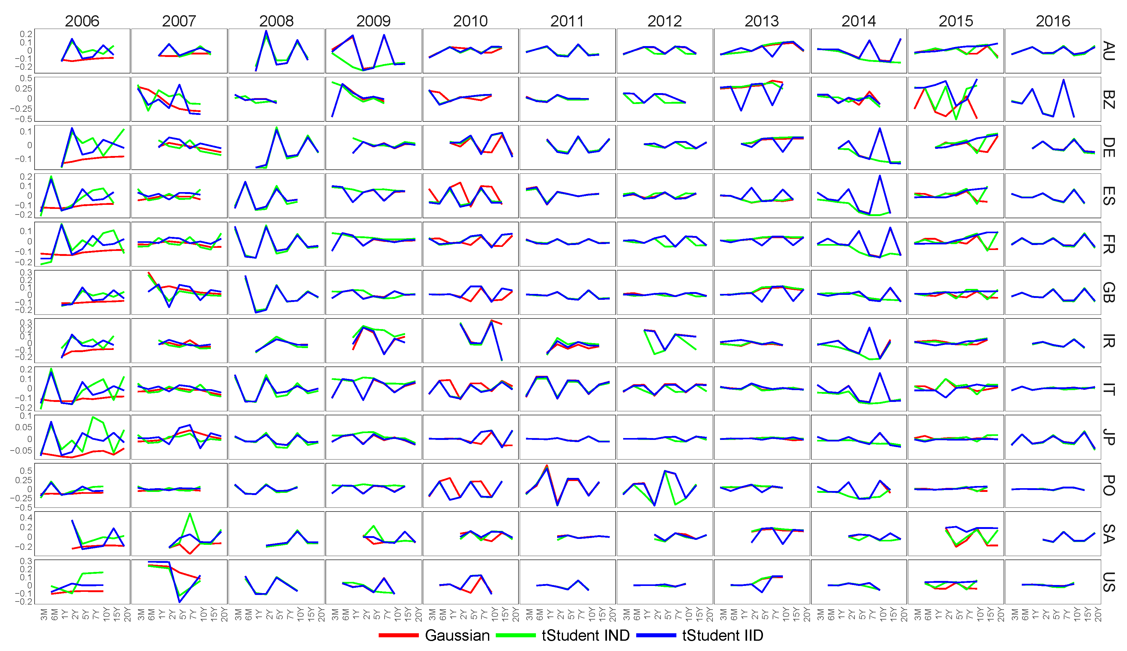
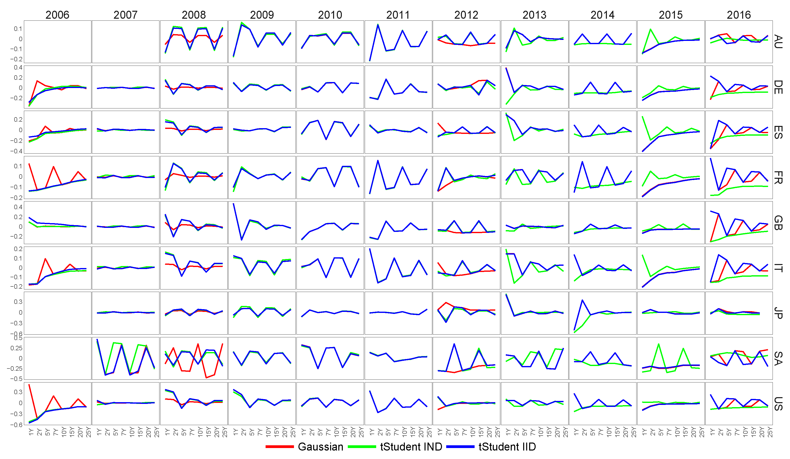
Figure 2 illustrates the first eigenvectors, which were obtained on yearly non-overlapping subsets of the D2 data corresponding to the period 2006–2016. The column-wise order of the panels illustrates the results for subsequent years, whereas the row-wise order corresponds to the country-specific sub-vectors. The term structure of the eigenvectors is given on the x-axis of the plots. We show the results for different frameworks: Gaussian PPCA (red line), t-Student IND PPCA (green line) and t-Student IND PPCA (blue line).
It is worth recalling that the eigenvectors obtained by different PPCA methodologies can be rotated, that is they may have the opposite signs (+/−1), but still provide similar directions. As an example, let us consider the plot of South Africa’s sub-eigenvector for the year 2007. The green and blue lines have the maximum point in 5Y maturity, whereas the red line indicates the minimum is the same point. If we multiply the red line by ‘−1’, all three lines would be consistently pointing towards the maximum in 5Y, but would indicate different magnitudes. Therefore, when analysing the resulting eigenvectors, we must distinguish between the difference in a rotation and the difference in the information given by the eigenvectors obtained by various PPCA methodologies.
The eigenvectors for the years 2008, 2011 and 2016 are very similar among all PPCA frameworks. The Gaussian PPCA and t-Student IID PPCA provide consistent features for the years 2009, 2012 and 2014, whereas the eigenvectors extracted using t-Student IND PPCA are smoother and shifted one term structure point backwards. The shift shows that t-Student IND PPCA indicates the heavier loadings on the shorter terms. For the year 2013, the features extracted using Gaussian and t-Student IND PPCA are both smoother across the term structure of a given country. The two t-Student methodologies agree in 2010 with the terms at maturities, which have the heaviest loadings. The vectors obtained by Gaussian PPCA highlighted longer points of maturities having the highest values.
With regards to the pre-crisis period 2006–2007, we notice strong differences between the t-Student and Gaussian PPCA frameworks. The values of the vectors provided by the non-robust methodology are consistent across the term structures and indicate non-varying decomposition of the features without pointing towards any subset of maturities. The contradicting information is given by t-Student PPCA methodologies, which highlight particular points on the term structures. It is an interesting outcome that illustrates the discrepancies between information provided by robust and non-robust frameworks and highlighting the importance of real data for adopting our proposed new methodology in such feature extraction in practice.
When analysing the country-specific panels year by year, one may remark that each methodology provides a consistent set of maturities for all examined countries, which have the highest loadings. The outcome gives us the intuition that the variability of the country-specific yield curves is determined by a common set of maturities across countries. The results differ on a yearly basis. In 2006, the eigenvectors point in the direction of the South African curve as the main source of the variability, which is complemented for most of the European countries. The source of the dominant variability of the dataset D2 in 2007 corresponds to the middle maturities from Brazil, the United Kingdom, South Africa and the United States.
In addition, one of the exceptional findings is the changed order of the degrees of freedom for the two t-Student PPCA frameworks in 2007. The optimal degrees of freedom chosen for t-Student IID PPCA in 2007 are higher than for the Student IND PPCA. One may expect that the reason for the increase in the degrees of freedom for the former methodology reflects the smaller variability of the yields. The first column of the panels in Figure S11 in the Supplementary Material illustrates the sovereign yields for 2006 and 2007 across various countries (row-wise) and maturities (the colours of the lines). The dynamics of the yields of European countries and the United States does not support this reasoning as the yields have started to decline in the middle of 2007 (the middle components of the United States yield even earlier). In addition, the optimal degrees of freedom for t-Student IND PPCA decreased in 2007, and consequently, the individual weights of the observations are lower in 2007 than in 2006. The assumed distribution in 2007 is more heavy-tailed than in 2006. The eigenvectors obtained by the two t-Student PPCA frameworks illustrated in Figure 2 are similar for most of the considered countries. The two methodologies agree that one of the main sources of the data’s variability is the middle tenors of the United States (U.S.) and United Kingdom (GB) yields. The strongest discrepancies between the results obtained by the two PPCA frameworks relate to the eigenvector components corresponding to Brazilian (BZ) and South African (SA) yields. The t-Student IID PPCA assumes the greater impact of the Brazilian yield on the variability of the dataset and loads more heavily on the middle terms of the yield, whereas t-Student IND PPCA selects the South African yield.
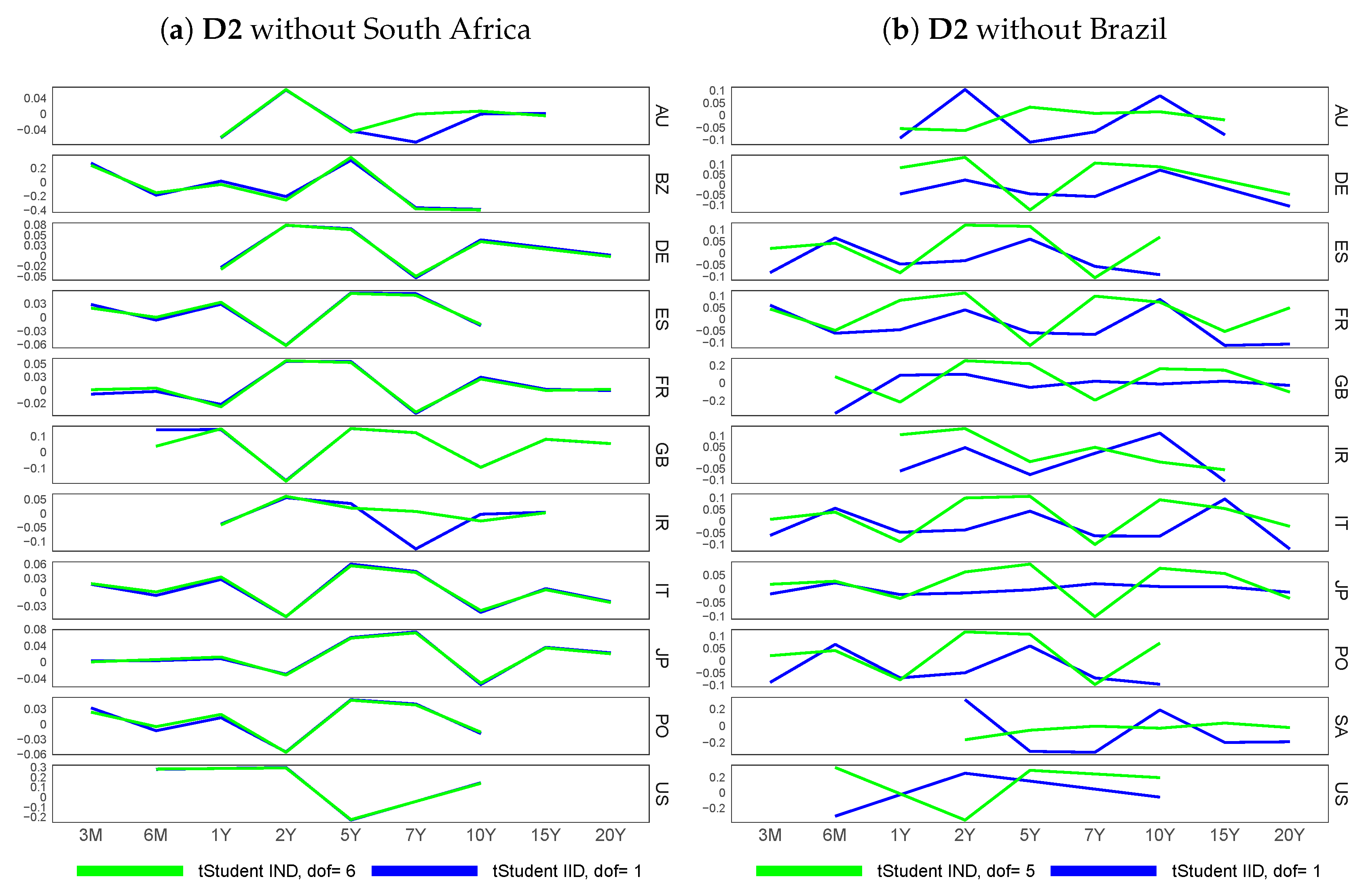
The Brazilian and South African yields are characterized by the moderate and strong missingness, respectively, as shown in the corresponding panels in Figure S5 in the Supplementary Material. The projections that are used to handle the presence of missing values in Brazilian and South African yields are determined by the conditional means of the corresponding distributions. We suspect that the source of this discrepancy is the difference in how the missing values present in the Brazilian and South African yields are projected. To verify this explanation, we check the eigenvectors and optimal degrees of freedom of the two t-Student frameworks for 2007 when the South African or Brazilian yields are removed from the dataset. The panels in Figure 3 show the obtained eigenvectors across the term structures (x-axis) and examined countries (row-wise). When either of the time series is removed from the dataset, the order of degrees of freedom reverts. In addition, when the South African yield is removed, the two PPCA methodologies provide consistent eigenvectors. Therefore, the South African yield is the source of the disagreement between the two t-Student frameworks in 2007.

6.2. Feature Extraction for Country-Specific Inflation-Linked Yield Curves

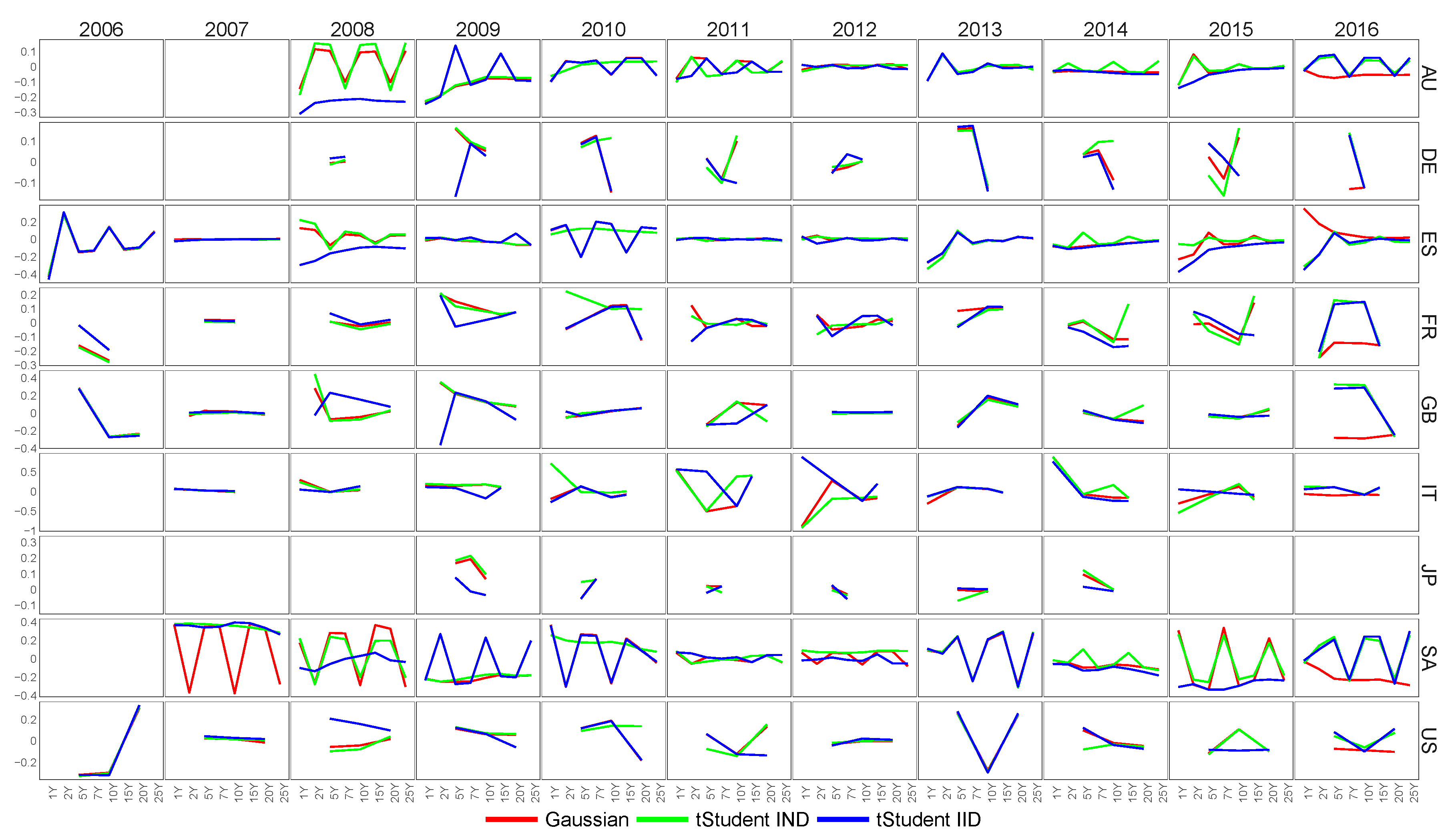
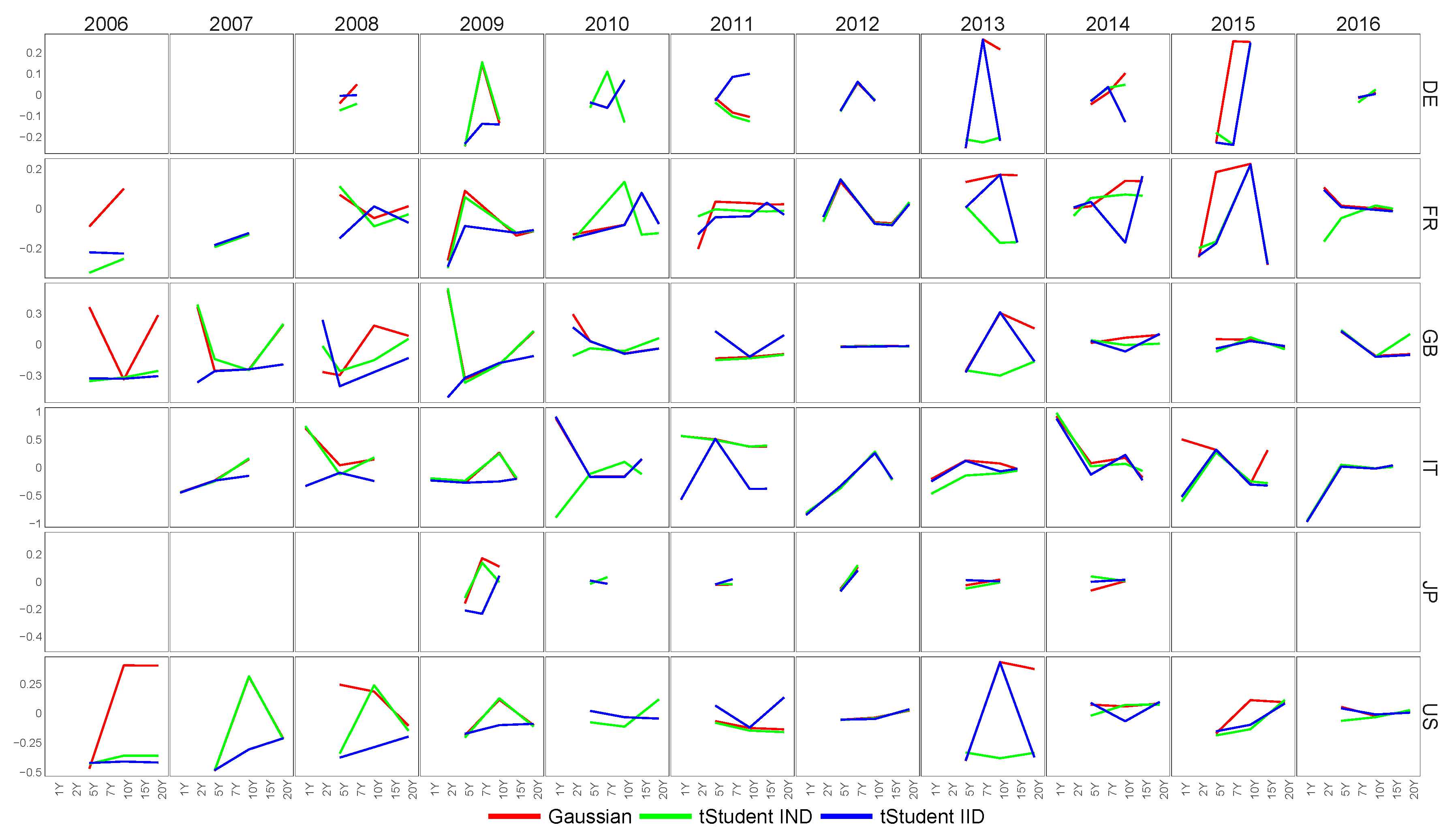
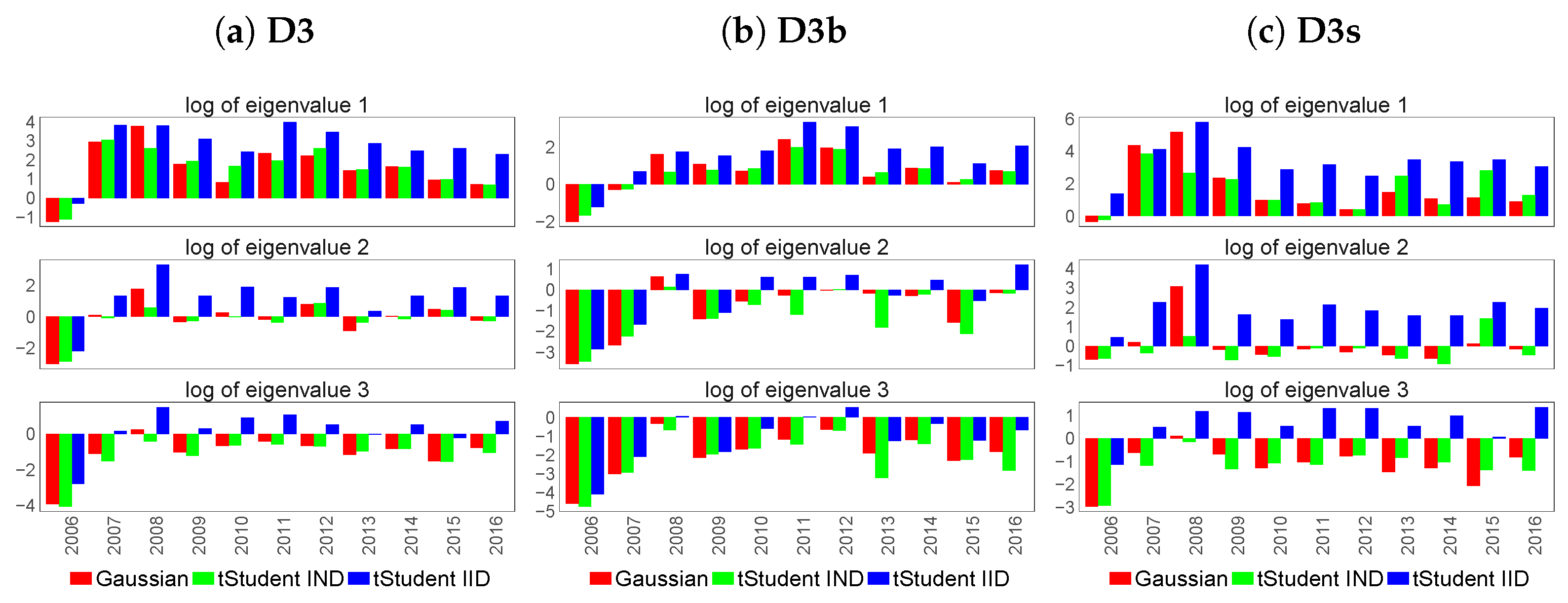
The eigenvectors of the datasets D3, D3b and D3s correspond to the country-specific inflation-linked yield curves and their term structures’ points. The first eigenvectors over different periods of time and across countries are illustrated in Figure 4, Figure 5 and Figure 6. The corresponding eigenvalues over years are also displayed in Figure 7a.
Interestingly, the eigenvectors of the sets D3 and D3b provide different information even though D3 contains all time series included in D3b in addition to two inflation-indexed swap yields, from Australia (AU) and Spain (ES). Surprisingly, the eigenvectors for swap curves in D3 are significantly different from their equivalents in the set D3s for Australia (AU) and Spain (ES).
The eigenvectors extracted from datasets D3 and D3b differ more significantly across the three examined PPCA methodologies than the corresponding results of the D2 dataset. If the choice of the fixed maturities was the same across these datasets, we would expect the information contained in eigenvectors of inflation-linked sovereign bond yield curves to be more consistent with the direction calculated from the conventional sovereign bonds. We notice smaller discrepancies when we compare the features between D3s and D2, especially when we analyse the yearly and country-specific patterns highlighting maturities with highest loadings.
The plots of eigenvalues are displayed in Figure 7a. The magnitude of the values is similar among the sets with various inflation-linked instruments. The yearly sequences of the second and third eigenvalues are consistent for the sets D3 and D3b, whereas the results for D3s are greater.
The choices of the degrees of freedom for two t-Student frameworks for three sets of inflation-linked rates are illustrated in Figure 8a. The IND t-Student PPCA exhibits more variability of the sequences of selected degrees of freedom, but it fluctuates around small values, indicating that robust weights are beneficial.

6.3. Feature Extraction for Macroeconomic Proxies of Euro Zone Activity

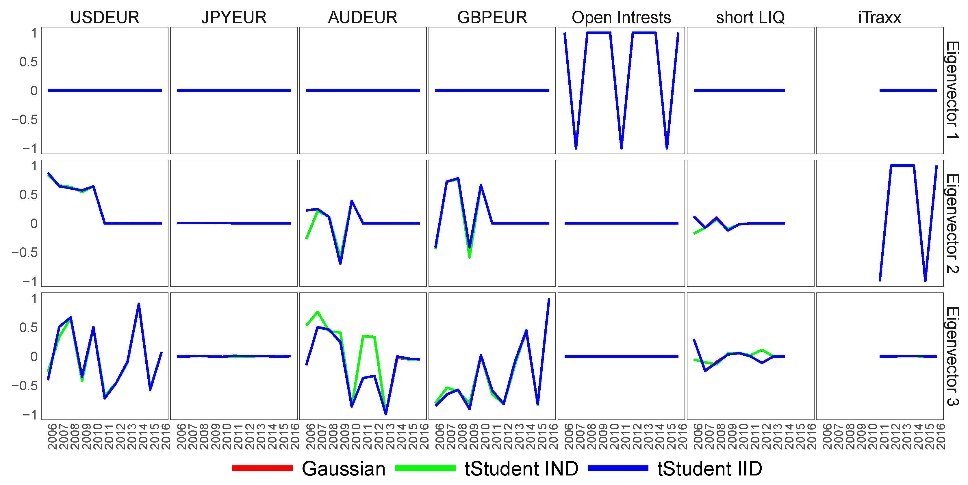
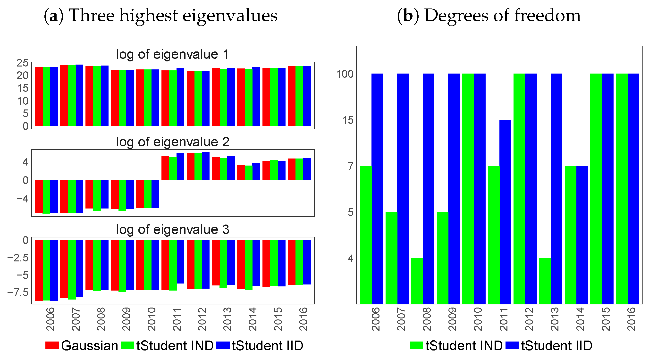
The features extracted from the dataset D4 are considered in this section. Since the instruments included in the dataset are vector-valued rather than matrix-valued, the resulting eigenvectors have the length corresponding to the number of instruments. Figure 9 shows the eigenvectors, which are extracted on yearly non-overlapping windows. The row-wise order of the panels illustrates the yearly sequences of the instrument-related elements of the three most significant eigenvectors, whereas the corresponding eigenvalues and selected degrees of freedom are shown in the panels of Figure 10b.
The two t-Student methodologies select the parameters of degrees of freedom, which differ significantly across years except for 2010–2012 and 2014–2016. The discrepancies are the highest among all examined datasets. Interestingly, the extracted features are very consistent across three PPCA frameworks and exhibit stronger differences only in the third eigenvector, which explains the insignificant portion of the data’s variability, as shown in Figure 10a.
The first eigenvector is indifferent across years and resembles a straight line for most of the instruments, except for the element that corresponds to the open interests of the Euro Bund features. The open interests are indicated as the most influential directions of the data’s variability.
Starting with 2011, we notice the increase in the importance of the second eigenvector, which is related to the presence of the Markit iTraxx Index, which started to be available from 2011. The presence of the index changes the yearly structure of the second eigenvector. Until 2011, its highest values corresponded to the exchange rates USDEUR, AUDEUR and GDPEUR, whereas after 2011, the only non-zero elements were related to the index.
Wit the dominance of the open interests over years in the variability of the set D4 given both by the values of corresponding elements of the eigenvector and the significance in the disproportion between the first and second eigenvalue, we can freely use only this dataset as a predictor of Euro Zone economic activity. The other time series contributes more negligibly to the shape of proxy indicators.

6.4. Similarity of Extracted Features across Various Financial Datasets

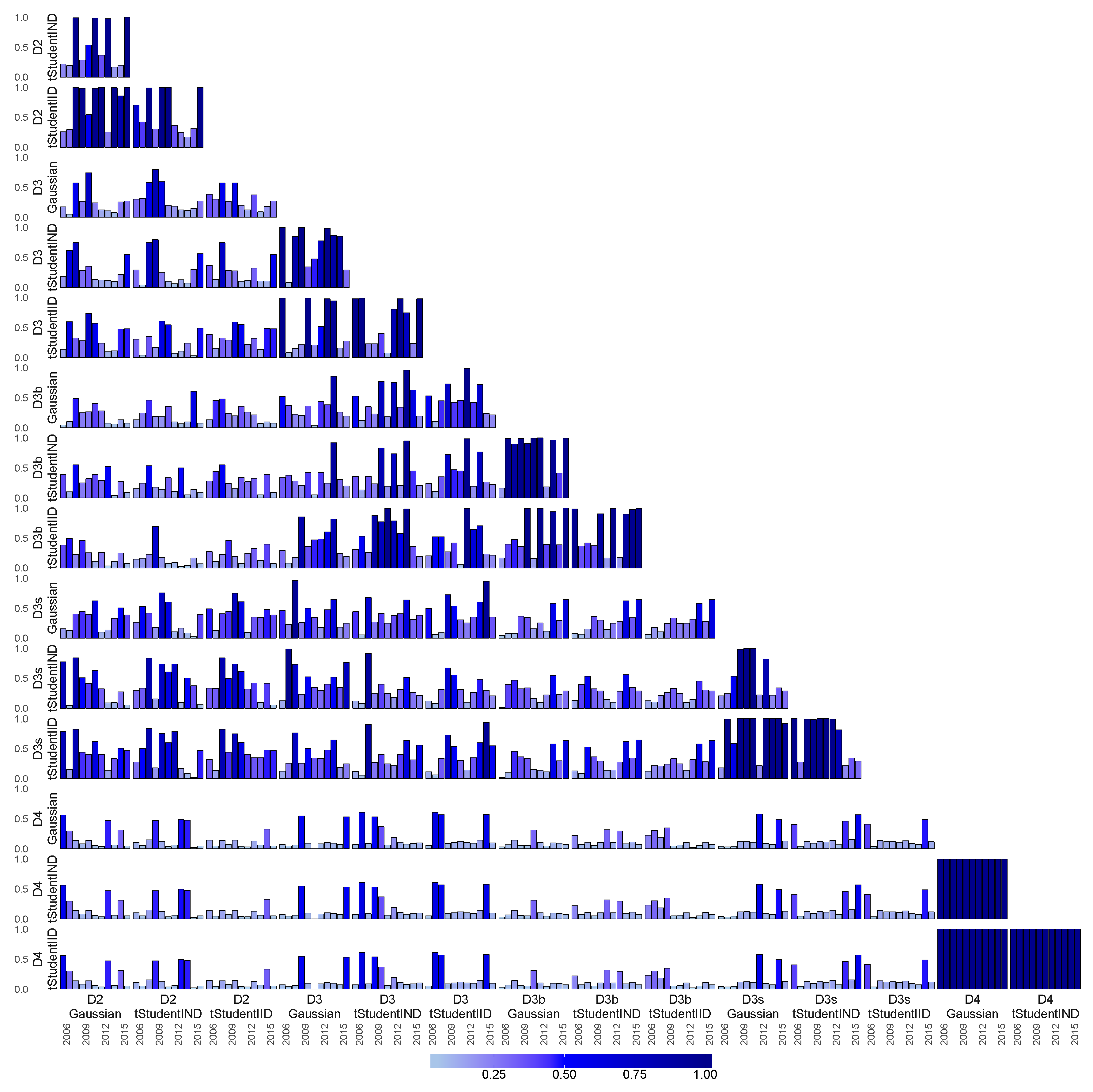
Having extracted spectral features via different PPCA methods, for a range of different financial datasets, we seek to study the statistical similarities among the resulting features. To achieve this, we analyse the strength of the matrix correlation between yearly features extracted from the datasets D2D4 discussed in Section 6.1, Section 6.2 and Section 6.3. This is performed using a multivariate generalization of the squared Pearson correlation coefficient Robert and Escoufier (1976) taken between two real m × n and m × l matrices A and B according to:
RV ( A , B ) = Tr A A T B B T Tr A A T 2 Tr B B T 2 .
Since the matrices with features are incorporated as exogenous factors of the extended Nelson–Siegel model for the Euro Libor yield curve, we need to ensure that the rows of matrices with features correspond to the term structure of Euro Libor curve. Consequently, we obtain the matrices with features that have consistent number of rows and are ready to calculate the correlation between them.
The last set of features extracted from datasets consists of proxies for Euro Zone credit, liquidity and foreign exchange risks and does not have a term structure, that is an extracted feature for yearly data is represented as a d e u r o -dimensional vector, where d e u r o denotes the number of scalar financial instruments in the dataset D4. Therefore, we replicate the vector with features across the terms structure in order to obtain a new d × d e u r o matrix, denoted as F t 4 . The new matrix has identical values across the term structure corresponding to the Euro Libor yield curve.
Figure 11 illustrates RVcoefficients across years (x-axis) between features extracted yearly from different examined datasets and using different PPCA frameworks. The bars correspond to pairwise RV coefficients for a given year between factors obtained using different methodologies and given different datasets. The row-wise and column-wise order specifies the coefficient over years for matrices and PPCA methodologies given by the row’s and column’s labels. The strength of similarity reaches values between zero and one, one being identical matrices. Both the height of the bars, as well as the colours correspond to the values of the RV coefficient.
The indicators of strong correlations between matrices are highlighted by values above 0.75 and support the previous discussion related to the eigenvectors of dataset M4 in Figure 9, which are consistent among examined PPCA methodologies. One may notice the strong yearly autocorrelation between features extracted from the dataset D4 within different PPCA methodologies highlighted by dark blue pars in the bottom right corner of the plots, which correspond by rows and columns to factors from the D4 set. In general, we see resulting higher values of the RV coefficient for factors from the same datasets. The strength of similarity between the factors across different sets is mostly weak, which indicates that our different classes of extracted exogenous factors may act as distinct sets of possible predictors to enter into our dynamic Nelson–Siegel term structure multi-factor models. As expected, the yearly factors from the D3 and D3b datasets usually exhibit high correlation due to their common attributes. Interestingly, we see strong autocorrelation between yearly factors from the D2 and D3s datasets, which is higher than between the factors from the country-specific sovereign yield curves dataset and other examined inflation-linked datasets.

7. Hybrid Multi-Factor Dynamic Nelson–Siegel Yield Curve Model of Euro Libor

In the following section, we examine the predictive and explanatory ability of extracted features from macroeconomic and financial datasets. Our goal is to verify whether the yearly market features provide us with additional explanatory power in the presence of the Nelson–Siegel yield regression state-space model. Given the extended model of Nelson–Siegel from Section 5, we use the yearly extracted features from datasets D2D4, discussed in Section 6, as exogenous factors. The features consist of the first eigenvectors of the sets’ covariance matrix calculated yearly.
Since the analysis of eigenvectors from the dataset D4 highlights that the Euro Bund Open Interests dominate the variance of the dataset, we utilise the daily time series of Open Interests as an exogenous variable in the observation equation. In addition, we examine the information contained in macroeconomic datasets with monthly or yearly observations, the raw time series of GDP, labour productivity, unemployment rates and CPI discussed in Appendix A.5. and A.3.1 in the Supplementary Material.
The analysed Euro Libor yield consists of two points at maturity 1Y, which correspond to either the 12-month Euro Libor rate provided by ICEor the 12-month Euro Libor swap rate. In the following section, we verify which of these two rates is the most informative in predicting and in-sample estimation of the Euro Libor yield model.

7.1. The Specification of the Optimal Models for EUR Libor Yield Dynamic Analysis

The selection of the set of assumptions for the models of the extended Nelson–Siegel class is a multiple step procedure. Therefore, before presenting the calibration results for the Euro Libor yield, we describe the four steps that we follow in order to find an optimal model per year.
Step 1: The choice of λ
The parameter λ specifies the shape of the Nelson–Siegel basis regression functions, which affects the concavity and convexity of the fitted yield curve model. The first step of the model selection is to select the best values of the parameter per year for all possible variants of the standard Nelson–Siegel model (all possible combinations of variants for matrices A , Q , R : diagonal or non-diagonal, heterogeneous or homogeneous, described in Section 5.4).
A grid of λ is fixed for every year and is specified by obtaining daily estimates of λ from the static daily fits of the static Nelson–Siegel model using non-linear regression for the period of time 2006–2016. The grid consists of 20 equally-spaced points between the 97.5 % and 2.5 % quantiles of the daily estimated λ. Next, we calculate the yearly estimates of the matrices A , Q , R for all values of λ, which belong to the grid, given different assumptions on the structure of the matrices. The estimates are obtained by maximising the likelihood of the corresponding Kalman filter estimations. This step provides us with 20 × 2 4 = 320 different Nelson–Siegel models per year: (the number of points on the λ-grid) × (diagonal or non-diagonal matrix A ) × (diagonal or non-diagonal matrix Q ) × (diagonal or non-diagonal matrix R ) × (heterogeneous or homogeneous matrix Q ) × (heterogeneous or homogeneous matrix R ). Hence, we have 20 possible different values of λ for each of the 2 4 variants of the Nelson–Siegel model. Within 20 values of λ, we select the one that provides the highest value of the marginalized likelihood obtained from the Kalman Filter for each variant of the Nelson–Siegel model.
Step 2: The specification of the baseline model: the assumptions on matrices A , Q , R per year
In the previous step, we selected the optimal values of λ for each of 2 4 examined variants of the Nelson–Siegel model per year. We use the Akaike Information Criterion (AIC) in order to compare between 2 4 different Nelson–Siegel models per year penalising for model complexity. The goal of this study is to examine the supplementary information provided by the various market features to the factors of the standard Nelson–Siegel model: the levels, slope and curvature of a yield. Hence, we first chose a baseline model for the Nelson–Siegel class of models, and as a next step, we plugged in additional factors, the yearly market features, to the model under the baseline’s model assumptions. We follow the two selection criteria for determining the Nelson–Siegel baseline model per year:
1. minAIC 
We select two standard Nelson–Siegel models with different restrictions on the static parameters that provided the lowest AIC;
2. diagAll 
We choose two models with a low complexity (the number of parameters to estimate) per year: the matrices of the model (10) are all diagonal; the covariance matrix Q is heterogeneous; the covariance matrix R is heterogeneous or homogeneous.
Step 2 left us with at most four models per year: the two models with the smallest AIC and the two models with low complexity.
Step 3: The choice of the yearly market features
The number of yearly country-specific market features is equal to 3 × 4 = 12 . The number four reflects the number of datasets D2D3s discussed in Section 6, and three is the number of different PPCA frameworks used to obtain the features: Gaussian PPCA, t-Student IND PPCA and t-Student IID PPCA. The analysis of the pairwise correlation discussed in Section 6.4 indicates the presence of strong correlations between some of the features. Therefore, we proceed with the preliminary feature selection methodology in order to remove the features that provide duplicated information. We choose as a yearly benchmark feature the first eigenvector from the dataset D2 obtained by the Gaussian PPCA framework. Every set of features contains at least the benchmark feature. Any other vector with features, the correlation of which with the benchmark feature, or any other feature already included in the analysis, is lower than 0.75 , is also added to the set of yearly market features. Hence, the sets of features might be of different sizes across years (maximum of nine) and consist of at least one element: the benchmark feature. The yearly choices of features are listed in Table S4 in Appendix F in the Supplementary Material. We denote the sets of models with different features by M2M3s, where the digits correspond to the datasets D2D3s.
We subset the obtained matrices of features from country-specific sovereign and inflation-linked yield curves in order to take only these elements, which correspond to Euro Libor term structure. If the datasets do not provide the feature for particular maturity, we set the corresponding elements of the new factor matrices to zero. Hence, the new F t 2 , F t 3 , F t 3 b and F t 3 s matrices with features extracted as the first eigenvectors of datasets D2D3s are d × d g o v t -, d × d i n f -, d × d i n f b - and d × d i n f s -dimensional, respectively, where d denotes the number of elements in the term structure of the Euro Libor curve, d g o v t denotes the number of country-specific sovereign yield curves, d i n f the number of country-specific bond-base filled with swaps inflation-linked yield curves, d i n f b the number of country-specific inflation-linked government bond yield curves and d i n f s the number of country-specific inflation-linked swap yield curves.
Furthermore, we separately examine the forecasting and calibration performance of the daily Euro Bund Open Interests since the time series of the instrument significantly dominate the variability of the dataset D4, as has been discussed in Section 6.3. The daily observations are added to the standard Nelson–Siegel models as the exogenous variable. The model that utilizes daily values of the Euro Bund Open Interests is denoted by M4.
The daily features of monthly and yearly time series of GDP, labour productivity and unemployment rate enter the base-line Nelson–Siegel model into the observation equation with the same magnitude across all maturities. Before the features are used for modelling, we verify that the columns of the loading matrix are collinear on a yearly basis. We detect the collinearity between the time series using the variance inflation factors test. The test discards all the positions in the datasets except the monthly-provided CPIs. We denote the model with the raw values of CPI, which are added to standard Nelson–Siegel models as an exogenous variable, by M1.
The standard Nelson–Siegel model is denoted by M0.
Step 4: The choice of the optimal model per year
After adding the additional explanatory variables (features from the datasets D2D3, daily observations of Open Interests or monthly observations of country-specific CPIs) to the standard Nelson–Siegel model, we use the Kalman filter to re-estimates the matrices A , Q , R under the reference model’s assumptions for all selected features. We compare the values of AIC in order to select the optimal model per year from the considered set of models: M0M4.

7.2. The Comparison of the Baseline Model Selection Methodologies

Tables S5 and S6 in Appendix F in the Supplementary Material compare the two baseline model selection methodologies described in Step 2 from the previous subsection within the considered two datasets of Euro Libor rates: with the one-year ICE Euro Libor rate or with the one-year swap Euro Libor rate, respectively. The table consists of the columns with yearly model’s specifications, its in-sample and out-of-sample performance. If the model belongs to the class of the extended Nelson–Siegel models, the last two columns describe which PPCA framework and the market-related dataset were utilized in the optimal model in a particular year.
The green colours of cells correspond to the years when the two baseline model selection methodologies agree on the best standard Nelson–Siegel model. The blue colour of cells correspond to the years when the extended Nelson–Siegel models chosen using the minAIC methodology obtained better in-sample performance than the extended Nelson–Siegel models with the lower complexity, whereas the yellow colour of cells corresponds to the years when it achieved better out-of-sample performance measured by mean square errors of 1-day, 1-week or 1-month predictions over the next calendar year. The upper index ‘*’ correspond to the yearly models belonging to the extended Nelson–Siegel family, which obtained poorer in-sample performance than the reference models from the standard Nelson–Siegel class.
Table S6 shows that the models that provide the best in-sample and out-of-sample fit for Euro Libor rates with the one-year ICE Euro Libor rate according to the minAIC criterion have mostly either non-diagonal transition matrix A ˜ or the covariance matrix R ˜ . The models chosen according to the selection methodology diagAll outperformed these models according to the in-sample calibration only in 2007 and according to the out-of-sample performance (one-day prediction) in 2008, 2009, 2011, 2012 and 2015.
The best models that are selected for Euro Libor rates with the one-year swap rate have mostly all matrices diagonal. The exceptions are the years 2006–2007 and 2014–2015. It is observed that for this dataset, we see particular years when the models with market features achieved poorer in-sample performance than their reference models. This is the case for the models selected according to minAIC in the years 2007, 2009 and 2010. What is more, we observe only three years when the models selected according to the minAIC methodology performed better than the models with lower complexity, the years 2006 and 2014–2015, and the improvement of the in-sample performance did not ensure better forecasting results.
In general, the differences between the models selected according to the two baseline model selection methodologies, which are highlighted by blue and yellow colours, are not significant in terms of their in-sample and out-of-sample performance. Considering the fact that the extended Nelson–Siegel models specified according to the minAIC methodology are more prone to calibrate the curve poorer than their simpler reference model, we drop this group of results from the following analysis.

7.3. In-Sample Fit of the Best Models for the Euro Libor Yield Curve

The calibration of the Euro Libor yield curve with either the 1Y ICE Libor rate or 1Y swap rate is the most accurate for the hybrid models from the extended Nelson–Siegel family, which significantly outperform the standard Nelson–Siegel model fits. We show that only for the short rates in the crisis period, the estimation of the yields carried by the standard Nelson–Siegel models is as good as by more complex models.
Table 2 provides the description of the extended Nelson–Siegel and the standard Nelson–Siegel models, which are selected on a yearly basis (the first column) as the best models for two Euro Libor yields, as well as their in-sample performance results. The column Model lists the acronyms of the best models corresponding to Step 3 in Section 7.1 (in case of the extended Nelson–Siegel family, it refers to a specific dataset of features). If applicable, the column PPCA indicates the PPCA framework used to obtain the market feature, the column R describes the structure of the covariance matrix R ˜ and, lastly, the column log λ informs about the value of the shape parameter of the Nelson–Siegel model. The models across the years have diagonal transition and covariance matrices and heterogeneous matrix Q as imposed by the baseline model selection methodology diagQ. The repeatedly-chosen structure of R ˜ is heterogeneous, allowing for differences in the magnitude of the latent vector’s elements’ variability. The smallest values of λ for the Euro Libor dataset with the 1Y swap rate are selected at the beginning and the end of the sample set, the years 2006 and 2007 indicating that the shape of the yield across the term structure is the flattest among examined periods. The highest values of the shape parameter correspond to the crisis period, 2008–2009, when the relative differences between the Euro Libor rates are the biggest. The shapes of the Euro Libor yield with the 1Y ICE Euro Libor rate do not follow this pattern, indicating a rapid decline of the parameter’s value in the middle of the sample period, in 2010.
Regardless of the different 1Y rates, we observe the agreement in the choice of the sets of assumptions on the static parameters for Nelson–Siegel and extended Nelson–Siegel models per year. Recall that the estimates of the parameters may still differ. The utilized market features mostly belong to the dataset D2 (the model M2 ) with the country-specific sovereign yields discussed in Section 6.1, except for the years 2008 and 2011, when the inflation-linked features from the dataset D3 are chosen to be more relevant. Most of the features selected for the extended Nelson–Siegel models are extracted using robust frameworks highlighting the importance of the information one may omit when it does not account for outliers in the data. The robust features are confirmed to provide more explanatory power in most of the cases.
The features from the dataset D2 in the year 2006 extracted by the two t-Student PPCA frameworks are characterized by a strong correlation reaching 0.7 . However, the independent t-Student methodology provides better in-sample performance. The reader may recall the discussion of the features from the dataset D2 in 2007 in Section 6.1, which are extracted using different PPCA frameworks. In 2007, all the features from the dataset D2 are very distant, but the smoother eigenvectors obtained by Gaussian PPCA are shown to obtain the explanatory power of the Euro Libor dynamics. In 2009, the most informative features are obtained using the independent t-Student PPCA framework, whereas the features from the same set next year obtained by two t-Student frameworks reveal high correlation and are similarly informative. The best features selected for 2011, which contain inflation-related information, are extracted using a non-robust methodology. In 2012, the Gaussian and t-Student IID PPCA provide similar eigenvectors, which have less explanatory power than the vectors obtained by t-Student IND PPCA. The opposite relation is present in 2013, when the results of the t-Student IND PPCA agree with the Gaussian PPCA, but capture fewer dynamics of corresponding Euro Libor yields. The features selected to model the yields in 2014 and 2013 are distant from the other choices of factors from the dataset D2, whereas the three vectors with features align in 2016.

7.3.1. The Calibration of the Euro Libor Yield Curve Using the 1Y ICE Euro Libor or 1Y Swap Rates

We observe that the difference of the time series of the rates at 1Y maturity impacts the resulting values of AIC, especially related to the standard Nelson–Siegel models’ fit. Before and during the crisis period, 2006–2010, the optimal models for the set with the 1Y swap rate obtained lower AIC values, whereas after 2012, this trend reverts. We want to verify if the information contained in different 1Y rates influences the calibration of the other terms of the Euro Libor yield. Figure 12 illustrates the yearly mean square errors of in-sample fit on the log scale across the term structure for different classes of the models and datasets. We define the mean square errors (MSE) for the considered models as a conditional mean of the difference between the observed data, y t , and the mean of the in-sample one-step ahead model forecast given by the Kalman filter, y t | t 1 = E [ y t | ψ , y 1 : ( t 1 ) ] given in Equation (12). Therefore, we calculate the mean square error of in-sample prediction (MSE) as the following average:
MSE : = E y t y t | t 1 y t y t | t 1 T
when T is the end of an in-sample period.
Recall that the only difference between the two datasets is a time series of the rate at 1Y maturity. Hence, all the results illustrated in Figure 12, except the ones corresponding to the 1Y rate, give us the intuition about which of the time series of the 1Y rate performs better in the calibration of the other tenors of the yield according to MSE. The column-wise order of the panels in Figure 12 corresponds to the calendar years, whereas the row-wise order of the panels refers to the results for different maturities. Every panel shows the MSE statistics for a particular year and rate. The grey bars present the results for the Nelson–Siegel models and the green ones for the extended Nelson–Siegel models. The colour of the borders corresponds to the different datasets: red, with the 1Y ICE Euro Libor rate; blue, with the 1Y swap rate. Comparing the two model classes, we observe that in all maturities and all years, the extended Nelson–Siegel family of models outperformed the classical standard Nelson–Siegel model. Hence, we can conclude that using market features benefited all tenors of the yield. The results do not provide the clear information about which rate is more informative for calibration of the yield in the considered period. The Nelson–Siegel model calibrated using the 1Y ICE Euro Libor rate more accurately estimates the rates at the 1M and 3M rate than the model fitted on the dataset containing the swap rate, with the exceptions in 2009 and 2012 for the 1M rate and 2010 and 2013 for the 3M rate. In general, the corresponding extended Nelson–Siegel model performs better in the calibration of the short end of the curve, when the one-year swap rate is present in the sample set. Only in 2011 does the hybrid model, which is fitted to the Euro Libor data with the 1Y ICE rate, outperform all other examined models. Recall that for the hybrid model estimated this year, we use the market features extracted from the dataset D3 with national inflation-linked yields.
The impact of the datasets on the calibration of the rates at 2Y–5Y maturity is the highest for 2006–2013 when the choice of the rate at 1Y maturity is year-specific. The middle terms, 7Y–20Y, are calibrated with the consistent accuracy regardless of the dataset. Furthermore, the rates at the maturities between 5Y and 10Y are similarly estimated by both classes of models. The rates at longest maturities are more successfully calibrated using the set containing the 1Y swap rate and market-related features.
The panels in Figure 13 show the resulting estimates of the Euro Libor rates at various maturities against their actual values over time. The column-wise order of the panels corresponds to different model classes and the datasets. The red colour of lines and shading correspond to the one-step ahead in-sample predictions given by y t | t 1 with corresponding 97.5 % confidence intervals, which are carried out on the dataset containing the 1Y ICE Euro Libor rate. The blue colour of lines and shading refer to the results for the dataset with the 1Y swap rate. Again, the displayed time series of the actual observations differ only for the rate at 1Y maturity. Hence, the reference observation over time in the panels corresponding to 1Y maturity is different for the results highlighted by red and blue colour. We can observe the aforementioned lower accuracy of the estimation given by the extended Nelson–Siegel model for the rates at short maturities, 1M and 3M for a crisis period. The gap between the actual observations and their predictions is visible for the hybrid models, and the corresponding confidence intervals are wide. On the other hand, the estimation given by the standard Nelson–Siegel model is very volatile (it jumps around the actual curve), which results in the comparable values of MSE as discussed above. In 2011, we see that the red extended Nelson–Siegel model is most accurate in estimating the 1M rate and is the worst for the 3M rate, whereas the pattern reveres for the extended Nelson–Siegel model fitted to the dataset with the swap rate. In addition, the panels that refer to the estimation of the rates at the longer maturities confirm that the extended Nelson–Siegel models should be used in the calibration of these rates.

7.3.2. Filtering of Latent Variables

Since the market features utilized in the extended Nelson–Siegel model are country-specific, we can analyse the results in terms of the strength of the influence of each examined country on the Euro Libor yield. The panels in Figure 14 and Figure 15 show the filtered values of the coefficient loadings, the latent state vector, over time given by the conditional mean β ˜ t | t from Equation (12) with corresponding 97.5 % confidence intervals, for the Nelson–Siegel and the extended Nelson–Siegel models over time, respectively. The illustrated time series are continuous only within a on- year period since the models are optimized every year. The blue colour of lines corresponds to the results associated with the dataset containing the 1Y swap rate. The dynamics of different components of the latent process are ordered by rows. The latent processes corresponding to level, slope and curvature have consistent dynamics for the two datasets. The only exception is the year 2010, when the levels of the latent processes shifted upwards when the 1Y ICE Euro Libor rate was present in the dataset. The reader may recall the model’s specification given in Table 2 and the rapid decrease of the shape parameter λ for this year. Hence, the reason for the shift is the significant change in the shape of the polynomials of the baseline Nelson–Siegel model for the dataset with the 1Y ICE Euro Libor rate. When considering the other country-specific components of the latent vectors of the extended Nelson–Siegel model, we may specify the list of countries that have the biggest impact on the Euro Libor yields across the examined period of time. Recall that the majority of the extended Nelson–Siegel models utilized the market features extracted from the datasets D2 with international sovereign yields. Only in 2008 and 2011, we use the features from the dataset D3 with inflation-linked yield curves
The country-specific time series that fluctuate around zero inform us that this specific country does not have an impact on Euro Libor yields. With the beginning of the crisis, we can observe that all the latent vectors corresponding to the European countries are characterized by non-zero dynamics with increased volatility, especially Portugal, Ireland, Spain and France. In addition, we see the increased activity of the processes corresponding to international markets, Australia, Japan and Brazil. The influences of other countries start to grow in 2009. However, for this year, we see the discrepancies between the information provided by the two different Euro Libor dataset. The dataset with the 1Y swap rate indicates the lack of influence of the French features, whereas the other set is the opposite. In recent years, we observed that most of the country-specific latent processes fluctuated around zero, which agrees with the previous remark that the fits provided by the standard Nelson–Siegel are closely informative for the fits of the models with the market features. We observe the higher shifts in the levels of the processes and the increase of their volatility in 2016.
In the majority of the considered periods, the difference between the inclusion of either the original 1Y Euro Libor rate or the swap rate affects only the magnitude of the movements of the country-specific processes, which is also linked to the different estimates of the models’ static parameters. Mostly, the two sets with different 1Y time series indicate a similar set of countries having an impact on the Euro Libor curve per year.

7.4. Forecasting Performance of the Extended Nelson–Siegel Models with Macroeconomic Factors

We use our models to produce term-structure forecasts at 1-day, 1-week and 1-month horizons, with encouraging results. The out-of-sample prediction of the Euro Libor yield with one and five steps ahead using extended Nelson–Siegel models outperforms the results provided by the standard models. When we increase the forecast horizon to one month, the discrepancies between the models from different families decrease and the Nelson–Siegel models provide a more accurate out-of-sample prediction, especially for shorter rates before 2011. What is more, the two model classes provide mostly consistent forecasts for the rates at middle term maturities, between 5Y and 20Y.
The prediction is performed on the one-day sliding window. Let us denote k as a forecasting horizon. We fit the models in the calendar year Y 0 (T observations) and take as an out-of-sample period the next calendar year, Y 1 ( T 1 observation points). Then, we predict the value of a rate in time T + t + k where t = 1 , , T 1 T , using the window of T consecutive observations from t , , T + t . Recall that the model was previously fitted to the data in time 1 , , T .
We use the Kalman filter in order to obtain the forecasting distribution. The Bayesian state-space framework allows us to obtain the forecasting distributions given by the Kalman filter, that is:
β ˜ T + t + k N c ˜ + A ˜ β ˜ T + t + k 1 , P T + t + k | T + t + k 1 y T + t + k N Λ ˜ T β ˜ T + t + k , F T + s + k .
where Λ ˜ T is a coefficient matrix with features up to the end of the in-sample period, the time T. Let us define the mean squared error of the out-of-sample prediction (MSEP) of k steps ahead as follows:
MSEP ( k ) = E y T + t + k E y T + t + k | y t : ( T + t ) y T + t + k E y T + y + k | y t : ( T + t ) T
Table 3 compares the forecasting performance of the examined models for different sets of sample data, with the 1Y swap rate and the 1Y ICE Euro Libor rate, respectively. The MSEP-related columns show the logarithms of the mean square errors of 1-day, 1-week and 1-month ahead predictions of the Euro Libor yield given the data from the next calendar year using the following conditional means: y t | t 1 , y t | t 5 , y t | t 22 . The yellow shading of the cells highlights the examples when the standard Nelson–Siegel model outperforms the hybrid model. The reader can observe that for the majority of years and the prediction horizons of one day and one week, the extended Nelson–Siegel models provide better out-of-sample forecasting performance and, hence, the information contained in the market features is meaningful for the out-of-sample prediction of the Euro Libor yield in addition to the in-sample calibration properties. The discrepancies between the two classes of models decline when we move to one-month ahead prediction, especially for the calendar years belonging to the pre-crisis and crisis period. The Nelson–Siegel model for one-month ahead prediction obtains better results for 2008 and 2011 when the 1Y swap rate is present in the dataset or only in 2011 when we use the corresponding swap rate.
Similarly to the in-sample analysis, we can study the tenor-specific out-of-sample forecasting performance of the models and verify if the quality of prediction is consistent across the tenors. We calculate the maturity and calendar year-specific MSEP for two datasets with different 1Y rates and two families of models. Figure 16, Figure 17 and Figure 18 illustrate the MSEP of 1-day, 1-week and 1-month predictions across different years and maturities. Regardless of the prediction horizon, the dependencies between the forecasting performance between the two classes of models, the standard and hybrid one, are the smallest for the rates at maturities between 2Y and 20Y. It is worth remarking that the prediction of the models calibrated on the dataset with the 1Y ICE Euro Libor rate provides in majority of cases the best results for the rates with maturities longer than 5Y for all prediction horizons. The exceptions is the year 2012 for the rate at 25Y maturity for prediction one-day and one-week ahead, when the extended Nelson–Siegel model calibrated on the dataset with the 1Y ICE rate obtained the poorest results among all examined models. Except for 2006 and 2012, the hybrid models exhibit significantly better forecasting properties of the rate at highest maturity.
With regards to the rates at short maturities, there is no clear pattern that indicates a model with the best prediction across years for a particular maturity. The rates at shortest maturities, 1M and 3M, are more successfully predicted one-step ahead by extended Nelson–Siegel models, except for 3M rates in 2008 and 2011 when the standard Nelson–Siegel model calibrated on the dataset with the 1Y ICE rate obtained the smallest MSEP. The similar pattern refers to the one-week prediction of these rates. However, when we move the forecasting horizon to one month, the less complex standard Nelson–Siegel models predict the short end of the Euro Libor curve at least as successfully as the hybrid models with the country-specific market features, especially for the years 2007–2011. Hence, the better performance one-month ahead prediction by the Nelson–Siegel models in 2008 and 2011 noted in Table 3 is a consequence of their more accurate forecast of the short end of the yields. In addition, the results of the one-month ahead prediction are characterized by the biggest discrepancies between the models calibrated on different Euro Libor datasets. It is not a surprising outcome since the inaccuracy of the prediction starts to dominate the results due to the long forecast horizon.
The panels in Figure S23 and Figure 19 show the one-step ahead out-of-sample prediction with corresponding 97.5 % confidence intervals across different maturities and for different models. Figure 19 illustrates the portions of the forecast when the biggest discrepancies are present. The blue colour of lines highlights the results for models calibrated on the dataset with the 1Y swap rate. Hence, the panels, which show the results for 1Y rate, consist of the different sets of data for models stressed by blue and red lines and shading. Recall that the out-of-sample prediction is conducted in the next calendar year from the year when a model was estimated. Hence, the results plotted in the panels of Figure S23 for the year Y 0 show the forecasting ability of a model calibrated in the year Y 1 . The most remarkable discrepancies of the various model’s forecast are noted for short maturities, 1M and 3M, and the longest maturity 25Y, especially for the year before 2013. We see substantial differences between two classes of models predicting the 1Y ICE Euro Libor rate. The extended Nelson–Siegel model more accurately captures the future movement of the rate. What is more, both hybrid models are characterized by the higher confidence of the results for 1Y rates as in the majority of case, the confidence intervals of the reference Nelson–Siegel model are wider.

8. Conclusions

In this work, we undertook three studies. We have shown the extensive analysis of the real data for what we believe is the most complete analysis of yield curve modelling to date in the literature, which has incorporated the country-specific financial and macroeconomic factors and comprehensively examined the variant of the models’ structure. Secondly, in order to conduct a parsimonious dimensionality reduction of big datasets, we extended the probabilistic principal component analysis in order to deal with missingness and robustness. We develop the novel PPCA methodology utilising the t-Student distribution in a new way and provide the efficient estimation framework, which is robust in the presence of missing data. We examined the derived framework both on synthetics and real data, conducting an excessive analysis of results.
As a third result, we combined these results together in order to create a hybrid multi-factor regression state-space model, and we assessed the performance of that on the real data with promising outcomes. The hybrid multi-factor model outperforms the standard Nelson–Siegel model in both forecast and in-sample analysis of Euro Libor yield.

Supplementary Materials

The following are available online at https://www.mdpi.com/2225-1146/6/3/34/s1. In Appendix A we provide the detailed overview of the time series analysed in this study and discussed in Section 2 along with their Bloomberg identifiers; in Appendix B we provide supplementary material to Section 6; in Appendix C we describe the EM algorithm for the standard Gaussian PPCA and its robust variant, robust Gaussian PPCA, as a complementary theory to Section 4; in Appendix D we show the proofs to the theorems related to the steps of EM algorithm and discussed in Section 4. The section is divided into the part corresponding to the EM algorithms for t-Student IND and t-Student IID PPCA, respectively; in Appendix E we illustrate the results of the synthetic data studies which we conducted to examine the sensitivity, convergence and robustness of various PPCA frameworks. We study the behaviour of the methodologies under various data characteristics such as dimensionality, sample size, proportions of missingness and perturbation and types of the data corruption; in Appendix F we detail the supplementary results to the real data case studies.

Author Contributions

D.T. is the main author of the manuscript and the implementations. The authors D.T. and G.W.P. contributed equally to methodological developments and data analysis.

Funding

This research received no external funding.

Acknowledgments

Dorota Toczydlowska and Gareth W. Peters would like to acknowledge the generous support of the Institute of Statistical Mathematics in Tokyo, Japan for providing the opportunity to visit, present and get feedback on aspects of this work.

Conflicts of Interest

The authors declare no conflict of interest.

References

  1. Abbritti, Mirko, Salvatore Dell’Erba, Antonio Moreno, and Sergio Sola. 2013. Global Factors in the Term Structure of Interest Rates. Washington, DC: International Monetary Fund. [Google Scholar]
  2. Akaike, Hirotogu. 1973. Information theory and an extension of the maximum likelihood principle. Paper presented at 2nd International Symposium on Information Theory, Tsahkadsor, Armenia, September 2–8. [Google Scholar]
  3. Ang, Andrew, and Monika Piazzesi. 2003. A no-arbitrage vector autoregression of term structure dynamics with macroeconomic and latent variables. Journal of Monetary Economics 50: 745–87. [Google Scholar] [CrossRef]
  4. Archambeau, Cédric, Nicolas Delannay, and Michel Verleysen. 2006. Robust Probabilistic Projections. Paper presented at the 23rd International Conference on Machine Learning, Pittsburgh, PA, USA, June 25–29; pp. 33–40. [Google Scholar]
  5. Armano, Giuliano, Michele Marchesi, and Andrea Murru. 2005. A hybrid genetic-neural architecture for stock indexes forecasting. Information Sciences 170: 3–33. [Google Scholar] [CrossRef]
  6. Bianchi, Francesco, Haroon Mumtaz, and Paolo Surico. 2009. Dynamics of the Term Structure of UK Interest Rates. SSRN Electronic Journal. [Google Scholar] [CrossRef]
  7. Borovykh, Anastasia, Sander Bohte, and Cornelis W. Oosterlee. 2017. Conditional Time Series Forecasting with Convolutional Neural Networks. arXiv, arXiv:1703.04691. [Google Scholar]
  8. Cairns, Andrew J. G., and Delme J. Pritchard. 2001. Stability of Descriptive Models for the Term Structure of Interest Rates with Applications to German Market Data. British Actuarial Journal 7: 467–507. [Google Scholar] [CrossRef]
  9. Candès, Emmanuel J., Xiaodong Li, Yi Ma, and John Wright. 2009. Robust principal component analysis? Neural Computation 21: 3179–213. [Google Scholar]
  10. Cao, Li-Juan, and Francis Eng Hock Tay. 2003. Support vector machine with adaptive parameters in financial time series forecasting. IEEE Transactions on Neural Networks 14: 1506–18. [Google Scholar] [CrossRef] [PubMed]
  11. Chen, Tao, Elaine Martin, and Gary Montague. 2009. Robust probabilistic PCA with missing data and contribution analysis for outlier detection. Computational Statistics and Data Analysis 53: 3706–16. [Google Scholar] [CrossRef] [Green Version]
  12. Chib, Siddhartha, and Bakhodir Ergashev. 2009. Analysis of Multi-Factor Affine Yield Curve. Journal of American Statistical Association 104: 1324–37. [Google Scholar] [CrossRef]
  13. Coroneo, Laura, Domenico Giannone, and Michele Modugno. 2016. Unspanned macroeconomic factors in the yield curve. Journal of Business & Economic Statistics 34: 472–85. [Google Scholar]
  14. Cuchiero, Christa, Claudio Fontana, and Alessandro Gnoatto. 2016a. A general HJM framework for multiple yield curve modeling. Finance and Stochastics 20: 267–320. [Google Scholar] [CrossRef]
  15. Cuchiero, Christa, Claudio Fontana, and Alessandro Gnoatto. 2016b. Affine multiple yield curve models. arXiv, arXiv:1603.00527v1. [Google Scholar]
  16. De la Torre, Fernando, and Michael J. Black. 2001. Robust Principal Component Analysis for Computer Vision. Paper presented at Eighth IEEE International Conference on Computer Vision, ICCV 2001, Vancouver, BC, Canada, July 7–14. [Google Scholar]
  17. Dempster, Arthur P., Nan M. Laird, and Donald B. Rubin. 1977. Maximum Likelihood from Incomplete Data via the EM Algorithm. Journal of Royal Statistical Society. Series B (Methodological) 39: 1–38. [Google Scholar]
  18. Diebold, Francis X., and Canlin Li. 2006. Forecasting the term structure of government bond yields. Journal of Econometrics 130: 337–64. [Google Scholar] [CrossRef]
  19. Ding, Chris, Ding Zhou, Xiaofeng He, and Hongyuan Zha. 2006. R1-PCA: Rotational Invariant L1-norm Principal Component Analysis for Robust Subspace Factorization. Paper presented at the 23rd International Conference on Machine Learning, ICML 2006, Pittsburgh, PA, USA, June 25–29; pp. 281–88. [Google Scholar]
  20. Mönch, Emanuel. 2008. Forecasting the Yield Curve in a Data-Rich Environment: A No-Arbitrage Factor-Augmented VAR Approach. Journal of Econometrics 146: 26–43. [Google Scholar]
  21. Eriksson, Anders, and Anton van den Hengel. 2012. Efficient Computation of Robust Weighted Low-Rank Matrix Approximations Using the L 1 Norm. IEEE Transactions on Pattern Analysis and Machine Intelligence 34: 1681–90. [Google Scholar] [CrossRef] [PubMed]
  22. Fang, Yi, and Myong K. Jeong. 2008. Robust Probabilistic Multivariate Calibration Model. Technometrics 50: 305–16. [Google Scholar] [CrossRef]
  23. Filipović, Damir, and Anders B. Trolle. 2013. The Term Structure of Interbank Risk. Journal of Financial Economics 109: 707–33. [Google Scholar]
  24. Geva, Tomer, and Jacob Zahavi. 2014. Empirical evaluation of an automated intraday stock recommendation system incorporating both market data and textual news. Decision Support Systems 57: 212–23. [Google Scholar] [CrossRef]
  25. Grbac, Zorana, and Wolfgang J. Runggaldier. 2015. Interest Rate Modeling: Post-Crisis Challenges and Approaches. New York: Springer. [Google Scholar]
  26. Gupta, Arjun K., and Nagar Daya K. 1999. Matrix Variate Distributions. Boca Raton: Chapman and Hall/CRC. [Google Scholar]
  27. Harvey, Andrew C. 1990. Forecasting, Structural Time Series Models and the Kalman Filter. Cambridge: Cambridge University Press. [Google Scholar]
  28. Huber, Peter J. 1964. Robust Estimation of a Location Parameter. The Annals of Mathematical Statistics 35: 73–101. [Google Scholar] [CrossRef]
  29. Huber, Peter J., and Elvezio M. Ronchetti. 2009. Robust Statistics. Wiley Series in Probability and Statistics; Hoboken: John Wiley & Sons, Inc. [Google Scholar]
  30. Hubert, Mia, Peter J. Rousseeuw, and Karlien Vanden Branden. 2005. ROBPCA: A New Approach to Robust Principal Component Analysis. Technometrics 47: 64–79. [Google Scholar] [CrossRef]
  31. Joslin, Scott, Marcel Priebsch, and Kenneth J. Singleton. 2014. Risk Premiums in Dynamic Term Structure Models with Unspanned Macro Risks. The Journal of Finance 69: 1197–1233. [Google Scholar] [CrossRef]
  32. Joslin, Scott, Kenneth J. Singleton, and Haoxiang Zhu. 2010. A New Perspective on Gaussian Dynamic Term Structure Models. Review of Financial Studies 24: 926–70. [Google Scholar] [CrossRef]
  33. Kalman, Rudolph E., and Richard S. Bucy. 1961. New Results in Linear Filtering and Prediction Theory. Journal of Basic Engineering 83: 95–108. [Google Scholar] [CrossRef] [Green Version]
  34. Karimalis, Emmanouil, Ioannis Kosmidis, and Gareth Peters. 2017. Multi Yield Curve Stress-Testing Framework Incorporating Temporal and Cross Tenor Structural Dependencies. Working Paper No. 655. London, UK: Bank of England. [Google Scholar]
  35. Ke, Qifa, and Takeo Kanade. 2005. Robust L1 Norm Factorization in the Presence of Outliers and Missing Data by Alternative Convex Programming. Paper presented at IEEE Conference on Computer Vision and Pattern Recognition, San Diego, CA, USA, June 20–25; pp. 739–46. [Google Scholar]
  36. Kercheval, Alec N., and Yuan Zhang. 2015. Modeling high-frequency limit order book dynamics with support vector machines. Quantitative Finance 15: 1–36. [Google Scholar] [CrossRef]
  37. Khan, Zia, and Frank Dellaert. 2003. Robust Generative Subspace Modeling: The Subspace t Distribution. Paper presented at British Machine Vision Conference 2003, Norwich, UK, September 9–11; pp. 1–17. [Google Scholar]
  38. Kwon, Yung-Keun, and Byung-Ro Moon. 2007. A Hybrid Neurogenetic Approach for Stock Forecasting. IEEE Transactions on Neural Networks 18: 851–64. [Google Scholar]
  39. Lange, Kenneth L., Roderick J. A. Little, and Jeremy M. G. Taylor. 1989. Robust Statistical Modeling Using the t Distribution. Journal of the American Statistical Association 84: 881–96. [Google Scholar] [CrossRef]
  40. Little, Roderick J. A., and Donald B. Rubin. 2002. Statistical Analysis with Missing Data, 2nd ed. Hoboken: John Wiley & Sons, Inc. [Google Scholar]
  41. Ludvigson, Sydney C., and Serena Ng. 2010. A Factor Analysis of Bond Risk Premia. In Handbook of Empirical Economics and Finance. Cambridge: National Bureau of Economic Research, pp. 313–72. [Google Scholar]
  42. Maronna, Ricardo. 2005. Principal Components and Orthogonal Regression Based on Robust Scales. Technometrics 47: 264–73. [Google Scholar] [CrossRef]
  43. Nelson, Charles R., and Andrew F. Siegel. 1987. Parsimoniuos Modeling of Yield Curves. The Journal of Business 60: 473–89. [Google Scholar] [CrossRef]
  44. Robert, Paul, and Yves Escoufier. 1976. A Unifying Tool for Linear Multivariate Statistical Methods: The RV- Coefficient. Applied Statistics 25: 257–65. [Google Scholar] [CrossRef]
  45. Rousseeuw, Peter J. 1985. Multivariate Estimation with High Breakdown Point. Mathematical Statistic and Applications 8: 37. [Google Scholar]
  46. Rousseeuw, Peter, and Victor Yohai. 1984. Robust Regression by Means of S-Estimators. In Robust and Nonlinear Time Series Analysis. New York: Springer, pp. 256–72. [Google Scholar]
  47. Sirignano, Justin. 2016. Deep Learning for Limit Order Books. arXiv, arXiv:1601.01987. [Google Scholar]
  48. Teichmann, Josef, and Mario V. Wüthrich. 2016. Consistent Yield Curve Prediction. The Journal of IAA 46: 181–224. [Google Scholar] [CrossRef]
  49. Tibshirani, Robert. 1996. Regression Shrinkage and Selection via the Lasso. Journal of the Royal Statistical Society. Series B (Methodological) 58: 267–88. [Google Scholar]
  50. Tipping, Michael E., and Christopher M. Bishop. 1999. Probabilistic Principal Component Analysis. Journal of the Royal Statistical Society 61: 622–61. [Google Scholar] [CrossRef]
  51. Tyler, David E. 1987. Statistical Analysis for the Angular Central Gaussian Distribution on the Sphere. Biometrika 74: 579–89. [Google Scholar] [CrossRef]
  52. Wright, Jonathan H. 2011. Term Premia and Inflation Uncertainty: Empirical Evidence from an International Panel Dataset. American Economic Review 101: 1514–34. [Google Scholar] [CrossRef]
  53. Xie, Pengtao, and Eric Xing. 2015. Cauchy Principal Component Analysis. arXiv, arXiv:1412.6506. [Google Scholar]
  54. Zhou, Zihan, Xiaodong Li, John Wright, Emmanuel Candes, and Yi Ma. 2010. Stable Principal Component Pursuit. Paper presented at IEEE International Symposium on Information Theory, Austin, TX, USA, July 13. [Google Scholar] [Green Version]
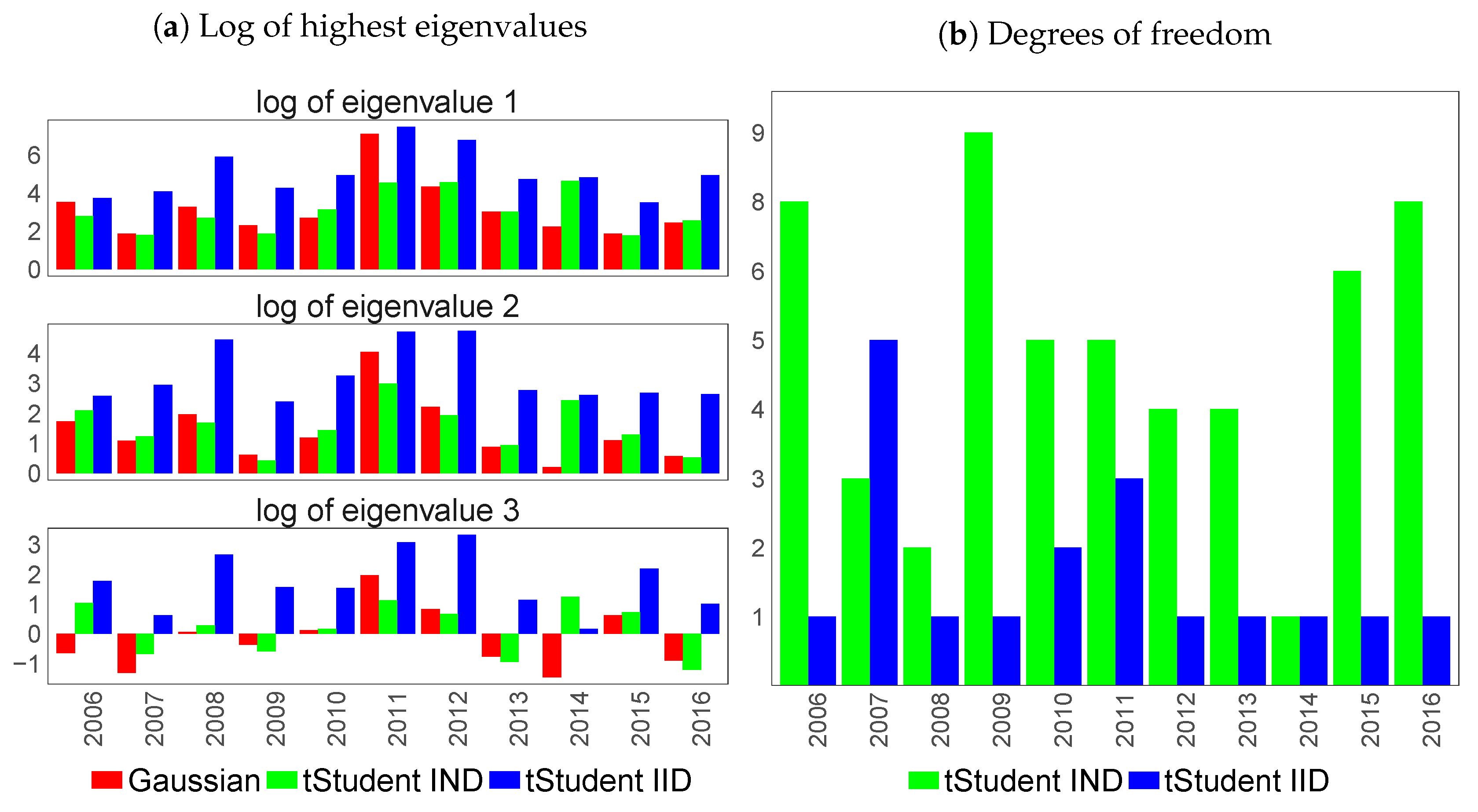
Figure 1. The left panel (a): the logarithms of the three highest eigenvalues of the covariance matrix; the‘right panel (b): the optimal values of the degrees of freedom for t-Student PPCA frameworks over years (x-axis) for the datasets D2, which consists of country-specific sovereign yields. IND, Independent; IID, identical and conditionally independent.
Econometrics 06 00034 g001
Figure 2. The first eigenvector of a covariance matrix for the D2 set of country-specific sovereign yield curves across different years (column-wise) partitioned into country-specific subvectors (row-wise) and their term structure (x-axis). The colours of lines correspond to different PPCA frameworks: Gaussian PPCA (red line), t-Student IND PPCA (green line) and t-Student IID PPCA (blue line).
Econometrics 06 00034 g002
Figure 3. The first eigenvector of a covariance matrix for the D2 dataset of country-specific sovereign yield curves without South African or Brazilian yields in 2007 partitioned into country-specific subvectors (row-wise) and their term structure (x-axis). The colours of lines correspond to different PPCA frameworks: t-Student IND PPCA (green line) and t-Student IID PPCA (blue line). The optimal degrees of freedom chosen for t-Student IND PPCA and t-Student IID PPCA are six and one, respectively.
Econometrics 06 00034 g003
Figure 4. The first eigenvector of a covariance matrix for the D3 set of inflation-linked mixed yield curves across different years (column-wise) partitioned into country-specific subvectors (row-wise) and their term structure (x-axis). The colours of lines correspond to different PPCA frameworks: Gaussian PPCA (red line), t-Student IND PPCA (green line) and t-Student IID PPCA (blue line).
Econometrics 06 00034 g004
Figure 5. The first eigenvector of a covariance matrix for the D3b set of inflation-linked bond-only yield curves across different years (column-wise) partitioned into country-specific subvectors (row-wise) and their term structure (x-axis). The colours of lines correspond to different PPCA frameworks: Gaussian PPCA (red line), t-Student IND PPCA (green line) and t-Student IID PPCA (blue line).
Econometrics 06 00034 g005
Figure 6. The first eigenvector of a covariance matrix for the D3s set of inflation-linked swap-only yield curves across different years (column-wise) partitioned into country-specific subvectors (row-wise) and their term structure (x-axis). The colours of lines correspond to different PPCA frameworks: Gaussian PPCA (red line), t-Student IND PPCA (green line) and t-Student IID PPCA (blue line).
Econometrics 06 00034 g006
Figure 7. The evolution of three highest eigenvalues of covariance matrix for the D3, D3b and D3s datasets of country-specific inflation-linked yield curves over years (x-axis).
Econometrics 06 00034 g007
Figure 8. The evolution of degrees of freedom for the D3, D3b and D3c datasets of country-specific inflation-linked yield curves over years (x-axis).
Econometrics 06 00034 g008
Figure 9. The first eigenvector of a covariance matrix for the D4 dataset of Euro Zone activity proxies across different years (row-wise) partitioned into country-specific subvectors (column-wise) and their term structure (x-axis). The colours of lines correspond to different PPCA frameworks: Gaussian PPCA (red line), t-Student IND PPCA (green line) and t-Student IID PPCA (blue line).
Econometrics 06 00034 g009
Figure 10. The evolution of three highest eigenvalues of the covariance matrix (a) and the evolution of degrees of freedom of the t-Student PPCA framework (b) over years (x-axis) for the datasets, which consist of country-specific sovereign yield.
Econometrics 06 00034 g010
Figure 11. The RV coefficients between various factors over different years (x-axis). The row-wise and column-wise orders of the panels correspond to the RV between different features extracted from sets of data using different PPCA methodologies in the same calendar year. The colours of bars refer to the value of the coefficient and the strength of similarity.
Econometrics 06 00034 g011
Figure 12. The logarithms of mean square errors (MSE) per year (column-wise) and tenor (row-wise) of the best Nelson–Siegel( grey colour of bars) and extended Nelson–Siegel (green colour of bars) models. The colour of the bar corresponds to different datasets, Euro Libor yield with the one-year ICE Euro Libor rate (red) or the one-year swap Euro Libor rate (blue).
Econometrics 06 00034 g012
Figure 13. The market observed yields of the Euro Libor rates at various maturities over time against the conditional mean of in-sample one-step ahead prediction y t | t 1 with corresponding predictive 97.5 % confidence intervals. The column-wise order of the panels corresponds to the results of the models that belong to different model classes, the standard Nelson–Siegel or the extended Nelson–Siegel family, and to the different set of the data Euro Libor yield with the one-year ICE Euro Libor rate (red lines and shading) or the one-year swap Euro Libor rate (blue lines and shading). The row-wise order of the panels corresponds to different terms of the yield.
Econometrics 06 00034 g013
Figure 14. The conditional mean of filtered latent states β t | t of the coefficient loadings with corresponding confidence intervals of the Nelson–Siegel models over time, which are optimal in term of the AIC criterion. The column-wise order of the panels corresponds to the models for the Euro Libor yield with the one-year ICE Euro Libor rate (the left column) or the one-year swap Euro Libor rate (the right column). The row-wise order of the panels corresponds to different terms of the yield.
Econometrics 06 00034 g014
Figure 15. The conditional mean of filtered latent states β ˜ t | t with corresponding confidence intervals of the extended Nelson–Siegel models over time, which are optimal in term of the AIC criterion. The column-wise order of the panels corresponds to the models for Euro Libor yield with the one-year ICE Euro Libor rate (the left column) or the one-year swap Euro Libor rate (the right column). The row-wise order of the panels corresponds to different terms of the yield.
Econometrics 06 00034 g015
Figure 16. The logarithms of mean squared errors of one-day prediction per year (column-wise) and tenor (row-wise) of the optimal Nelson–Siegel (NS) and Extended Nelson–Siegel (ENS) models (x-axis). The colours of the bar correspond to different datasets, Euro Libor yield with the one-year ICE Euro Libor rate (red) or the one-year swap Euro Libor rate (blue).
Econometrics 06 00034 g016
Figure 17. The logarithms of mean squared errors of one-week prediction per year (column-wise) and tenor (row-wise) of the optimal Nelson–Siegel (NS) and Extended Nelson–Siegel (ENS) models (x-axis). The colours of the bar correspond to different datasets, Euro Libor yield with the one-year ICE Euro Libor rate (red) or the one-year swap Euro Libor rate (blue).
Econometrics 06 00034 g017
Figure 18. The logarithms of mean squared errors of one-month prediction per year (column-wise) and tenor (row-wise) of optimal NS and ENS models (x-axis). The colours of the bar correspond to different datasets, Euro Libor yield with the one-year ICE Euro Libor rate (red) or the one-year swap Euro Libor rate (blue).
Econometrics 06 00034 g018
Figure 19. The Euro Libor rates at 1M, 3M, 1Y and 25Y maturities (black line) with the one-step ahead out-of-sample prediction given by the conditional mean y T + s + 1 | T + s with the corresponding predictive 97.5 % confidence intervals over the considered period. The column-wise order of panels corresponds to different classes of models, the Nelson–Siegel or extended Nelson–Siegel model, calibration on two datasets with different 1Y rates (colours of lines and shading). The row-wise order corresponds to the evolution of rates at different maturities over time.
Econometrics 06 00034 g019
Table 1. The list of collected financial and macroeconomic time series investigated in the study. The first three columns of the table correspond to the name, sector category and frequency of the quotes of an instrument. The rest of the columns indicate country-specific availabilities of the collected data. The Bloomberg identifiers of the data are listed in Tables S2 and S3 in Appendix A in the Supplementary Material.
InstrumentCatFreq.Availability
EUDEFRPOESITIRGBJPU.S.AUBRSA
Libor Curve daily
Sovereign CurveGOVdaily
Inflation CurveINFdaily
FXRatesFXdaily
CPIINFmonthly
GDPPRDyearly
Unemployment RatesPRDyearly
Labour ProductivityPRDyearly
German Bund OILIQdaily
Euro Repo and Euribor 3MLIQdaily
Markit iTraxx 5YCRdaily
Table 2. The model specification and in-sample statistics for the best standard Nelson–Siegel model and the extended Nelson–Siegel models chosen by diagAll per calendar year (the first column) for the two sets of Euro Libor yield: with the 1Y ICE Euro Libor rate or the 1Y swap rate. The column Model lists the acronyms of the best models corresponding to Step 3 in Section 7.1 (in the case of the extended Nelson–Siegel family, it refers to a specific dataset of features). The column PPCA indicates the PPCA framework used to obtain the market feature (1, Gaussian PPCA; 2, t-Student IND PPCA; 3, t-Student IID PPCA). The column R describes the structure of the covariance matrix R ˜ , and the column log λ informs about the value of the shape parameter of the Nelson–Siegel model. The columns l, AIC and logMSE provide the yearly values of measures of the estimation accuracy: the log-likelihood of the Kalman filter, the Akaike information criterion statistics from Equation (14) and the logarithm of the mean squared error from Equation (15). hete, heterogeneous.
Year1Y ICE Euro Libor Rate1Y Swap Rate
ModelPPCAR log λ lAIClog MSEModelPPCAR log λ LAIClog MSE
2006M0 hete−1.425922.73−11,843.46−3.99M0 hete−1.426164.91−12,327.83−4.07
M22hete−1.427898.12−15,794.25−4.30M22hete−1.428101.40−16,200.80−4.36
2007M0 hete−0.765965.95−11,929.90−3.16M0 hete−0.966256.79−12,511.59−3.23
M21hete−0.767305.62−14,609.24−3.67M21hete−0.967114.59−14,227.19−3.99
2008M0 hete−0.523331.25−6660.50−3.03M0 hete−0.483581.24−7160.47−2.64
M33hete−0.524841.08−9680.15−3.98M33hete−0.485077.73−10,153.47−3.81
2009M0 hete−0.525184.72−10,367.44−4.27M0 hete−0.485679.58−11,357.15−4.47
M22hete−0.526764.61−13,527.22−5.64M22hete−0.487108.11−14,214.22−5.77
2010M0 hete−2.185422.09−10,842.19−3.66M0 hete−0.646027.31−12,052.63−4.31
M22hete−2.187650.23−15,298.46−6.20M22hete−0.647450.24−14,898.48−5.81
2011M0 hete−0.524357.33−8712.66−3.40M0 hete−0.565191.04−10,380.08−4.26
M31hete−0.526502.81−13,003.63−5.19M31hete−0.566513.74−13,025.47−5.07
2012M0 hete−0.524368.44−8734.87−2.90M0 hete−0.744377.26−8752.52−4.66
M22hete−0.527773.09−15,544.17−6.23M22hete−0.747535.36−15,068.73−5.76
2013M0 hete−0.835738.36−11,474.72−4.69M0 hete−0.745390.17−10,778.33−5.29
M23hete−0.837854.03−15,706.06−6.55M23hete−0.748128.64−16,255.27−6.72
2014M0 hete−0.915225.34−10,448.68−4.43M0 hete−0.965638.23−11,274.46−5.40
M22hete−0.918462.48−16,922.96−6.42M22hete−0.968525.73−17,049.46−6.47
2015M0 hete−0.996243.56−12,485.13−4.93M0 hete−0.966639.60−13,277.21−5.87
M21hete−0.998886.02−17,770.05−6.63M21hete−0.968927.51−17,853.02−6.67
2016M0 hete−0.995150.36−10,298.73−4.69M0 hete−1.096108.33−12,214.66−5.54
M21hete−0.998595.78−17,189.57−6.98M21hete−1.098908.23−17,814.46−7.15
Table 3. The forecasting performance of the best extended Nelson–Siegel and Nelson–Siegel models for the Euro Libor yield curve with 1-year ICE Euro Libor rate and the 1-year swap rate per year.
Year1Y ICE Euro Libor Rate1Y Swap Rate
Modellog MSEPModellog MSEP
1D1W1M 1D1W1M
2006M0−3.93−3.78−2.94M0−4.01−3.85−3.26
M2−6.35−4.93−3.41M2−6.20−4.96−3.59
2007M0−1.95−2.09−1.88M0−2.24−2.36−1.75
M2−4.90−3.33−2.01M2−4.92−3.42−1.94
2008M0−4.10−3.74−2.81M0−4.43−3.89−2.65
M3−5.70−3.96−2.57M3−5.46−3.56−2.05
2009M0−3.77−2.77−1.26M0−3.80−2.76−1.38
M2−5.60−3.07−1.45M2−5.66−3.16−1.53
2010M0−2.29−2.29−1.78M0−4.18−3.62−2.34
M2−5.52−3.69−2.22M2−6.02−4.51−2.68
2011M0−2.90−2.90−2.23M0−3.49−3.18−2.12
M3−6.16−4.23−1.99M3−6.02−3.98−1.70
2012M0−3.86−3.69−3.03M0−4.79−4.43−3.52
M2−7.31−5.79−4.13M2−7.26−5.82−4.17
2013M0−4.30−4.24−2.97M0−4.91−4.81−2.85
M2−7.18−5.74−3.73M2−7.19−5.88−3.74
2014M0−4.86−4.42−2.92M0−5.83−4.93−2.92
M2−7.05−5.25−3.17M2−7.01−5.21−3.01
2015M0−4.34−4.17−3.55M0−5.32−5.05−3.97
M2−7.77−6.31−4.49M2−7.69−6.29−4.38