1. Introduction
Skill-biased technological change (SBTC) is the leading hypothesis in the literature to explain the rise in wage inequality.
3 It is often argued that for SBTC to be a compelling explanation of labor market trends, the trends have to be similar across different countries having access to the same technology (
Card and Lemieux 2001), provided institutions—or other developments—do not cause different trends. SBTC explains a rise in wage dispersion both between education groups (rising education premia) and within education groups (growing returns to experience and unobserved skills). In addition to SBTC, the literature on the rise in wage inequality discusses the role of the supply of skilled workers,
4 changes in institutions such as the decline in unionization and changes in the minimum wage,
5 the rise of international trade
6 or the increase in workplace heterogeneity (
Card et al. 2013).
In contrast to technology based explanations for the U.S.,
DiNardo et al. (
1996) and
Lemieux (
2006a) argued that increasing wage inequality in the 1980s and the early 1990s can be explained to an important part by changing labor market institutions, i.e., falling real minimum wages and deunionization, and a changing composition of the workforce. If institutional differences matter, one would not necessarily expect to see similar patterns in wage growth and polarization for different countries. The evidence for Germany regarding the role of the decline in unionization in explaining the increase in wage inequality is mixed.
Dustmann et al. (
2009) and
Biewen and Seckler (
2017) found a strong role of deunionization on explaining the rise in wage inequality, while
Card et al. (
Card et al. 2013) and
Antonczyk et al. (
2010) pointed to the growing heterogeneity in wage setting at the firm level as key drivers.
Dustmann et al. (
2014) pointed out that wage inequality rose strongest after 1995 among workers covered by collective bargaining. The study attributes the rise in wage inequality to a decentralization of wage setting to the firm level among firms covered by collective bargaining.
Autor et al. (
2008) argued that changing minimum wages and institutions in the U.S. are unlikely to explain the continuing trend of increasing wage inequality in the upper part of the wage distribution.
SBTC has been refined by the task approach introduced by
Autor et al. (
2003) which implies polarization of employment and which may also be consistent with polarization of wages (
Autor 2013;
Autor and Dorn 2013;
Autor and Handel 2013;
Autor et al. 2008).
Autor et al. (
2003) proposed as a nuanced version of SBTC that technological change can have a “polarizing” effect on the labor market rather than uniformly favoring skilled workers. That is, technological change—for example, computerization—favors more highly skilled workers relative to less skilled routine-manual and routine-cognitive workers. At the same time, various studies find a disproportionate growth of employment for low-wage jobs (often involving non-routine-manual work) relative to medium-skilled jobs. Altogether, starting in the 1990s, the distribution of jobs has been “polarizing” with faster employment growth in the highest and lowest-paying jobs and slower growth in the middling jobs.
7 However, the relationship between changes in employment and wages is less clear.
Autor and Dorn (
2013) developed a theoretical model where the wage effects at the bottom of the wage distribution are ambiguous, because they depend upon whether low-skilled jobs are complements or substitutes of high-skilled jobs. Thus, technology driven polarization in employment may also be consistent with rising wage inequality at the bottom of the wage distribution.
From the late 1970s to the mid-1990s, trends in wage inequality differed strongly between the U.S. and Germany. The U.S. experienced in the 1980s a uniform increase of wage inequality along the entire wage distribution (
Katz and Autor 1999), while the increase in wage inequality in Germany was restricted to the upper part of the wage distribution (
Dustmann et al. 2009;
Fitzenberger and Wunderlich 2002). In Germany, the increase in wage inequality in the lower half of the wage distribution began in the mid-1990s (
Dustmann et al. 2009;
Dustmann et al. 2014,
Biewen et al. 2017) and there was a uniform increase of wage inequality along the entire wage distribution until 2010 (
Biewen et al. 2017;
Dustmann et al. 2014).
Autor et al. (
2008) provided evidence for a polarization of wages in the U.S. during the 1990s such that wage inequality only continued to rise in the upper part of the wage distribution. Furthermore,
Autor and Dorn (
2013) found that employment and wages in low-skill service jobs, which involve non-routine manual tasks and which pay low wages, have grown considerably since the early 1990s. In contrast,
Dustmann et al. (
2009) for Germany and
Goos et al. (
2014) for 16 EU countries found no evidence for this. Hence, despite similar employment changes, wage inequality has been changing differently in the U.S. compared to European countries. These differences motivate our paper which takes a fresh look at the comparison of trends in wage inequality in the U.S. and in Germany using a unified framework of analysis.
As its key contribution, our study accounts for cohort effects. We define these as effects which are associated with the time a specific cohort was born and which have a permanent effect on this specific cohort.
Card and Lemieux (
2001) allowed for imperfect substitutability between younger and older workers to explain the fact that the large increase of the wage gap between young college- and high-school graduates is mainly driven by a slowdown in the growth of college graduates in the U.S. during the 1980s. This resulted in a stronger rise of the college–high-school wage gap for younger workers compared to older workers. In a similar vein,
Glitz and Wissmann (
2017) argued for Germany that the slowdown in the decline of the share of low-education relative to medium-education employment can explain the the rise in the wage differential between these two education groups.
Carneiro and Lee (
2011) reanalyzed the rising college–high-school premium and provide evidence that about half of the increase reported may be explained by an increased quality of college graduates during this period, which again reflects a cohort effect. Even though SBTC may have a bias in the age/cohort dimension, most of the recent literature on trends in wage inequality (see, e.g.,
Autor et al. 2008;
Dustmann et al. 2009) restricts itself to a comparison of cross-sectional age or experience profiles in different years.
This paper builds on the empirical framework developed by
MaCurdy and Mroz (
1995) to investigate the importance of age, time, and cohort effects on wages in light of the linear relation between the three variables. We implement a test of the separability of the three effects using standard errors robust against correlation across time and cohort, and we discuss identification of the linear effects. Based on this approach, we examine trends in wage inequality within and across cohorts of full-time working men in the U.S. and Germany by describing a set of quantiles. Wage dispersion in both countries has been rising since the end of the 1970s. While there is strong evidence of rising wage inequality in both economies, we confirm wage polarization only for the U.S. after 1985 and for Germany prior to 1985.
Our main findings are as follows: Based on the estimated conditional time trends, we confirm widening wage dispersion in both the U.S. and Germany between 1979 and 2004. This is the case if we consider trends for wages at the median between education groups as well as quantile specific time trends within education groups. However, there are various distinct patterns. For the U.S., we find that time-trends at the median are more positive for high-education workers than for less educated workers throughout the entire period—the medium-low-education gap ceases to increase during the 1990s. Moreover, time-trends within both the group of low- and medium-education workers start polarizing at the end of the 1980s, while within wage dispersion for high-education workers steadily increases. Trends in Germany are more difficult to interpret. We find little evidence for wage polarization in Germany and growing inequality among low- and medium-education workers after 1985. Moreover, we see a large role played by cohort effects in Germany—suggesting a role for supply-side effects or an interaction with institutions in Germany—while we find smaller cohort effects of opposite sign in the U.S. In addition to wage trends, we analyze the changes in the skill composition of the workforce and find strong parallel movements between the U.S. and Germany.
The remainder of the paper proceeds as follows:
Section 2 describes the two data-sets. The third section presents the basic facts of wage growth and wage dispersion for the U.S. and Germany.
Section 4 introduces our version of the
MaCurdy and Mroz (
1995) approach. The corresponding empirical results are presented in
Section 5. Finally,
Section 6 provides our conclusions. The
Supplementary Material contains graphical illustrations of our estimation results. Detailed estimation results are available upon request.
2. Data
The data we use for our analysis are the U.S. Current Population Survey (CPS) and the German IAB employment subsample (IABS) [while our paper refers to Germany, recall that our analysis is restricted to West Germany]. We focus on male workers who are between 25 and 55 years old. This avoids interference with ongoing education and early retirement.
2.1. CPS for U.S.
The U.S. data used for this analysis are from the Current Population Survey, Outgoing Rotation Groups (CPS-ORG) from 1979–2004. The CPS-ORG data contain wage and salary information for respondents during the month they leave the basic (monthly) survey. Wages are inflated to 2004 dollars using the CPI-U-RS. Workers’ calculated hourly wage rates are either the reported hourly wage (for the 60 percent of workers paid on that basis) or weekly earnings divided by weekly hours (for the other 40 percent of workers). For the latter group, earnings per week divided by the usual hours per week was used, unless information on usual hours per week was missing (in 2004, for example, the figures were missing for 5 percent of workers not paid on an hourly basis). In that case, the analysis used the number of actual hours worked in the previous week to construct hourly wages. While that procedure minimizes the number of workers excluded from the analysis, it introduces some noise into the calculated hourly rate of pay because the actual hours worked last week may differ from usual hours worked per week. For roughly 15 percent of workers not paid on an hourly basis, the number of actual hours worked the previous week was different from the usual hours per week. Most often, those workers indicated that they worked part time in the previous week for various reasons, but usually worked full time. The U.S. Census Bureau imputed data on hourly wage rates, usual weekly earnings, and usual hours worked per week were used in the analysis. Over the sample period, the percentage of workers with imputed wage data has increased and was 31 percent in 2004.
We consider male workers from the sample who (normally) work full time. The education level between 1979 and 1989 is measured as a categorical variable with three values regarding the years of schooling completed:
| (U) 12 years or less of schooling | (low-education) |
| (M) 13 to 15 years of schooling | (medium-education) |
| (H) 16 years or more of schooling | (high-education). |
These categories are defined in a slightly different way after 1990 due to changes in the CPS: (U) having a high school diploma or less and not having attended college; (M) having attended college but not having received a degree; and (H) having at least a college degree. Age is measured continuously (in years). Observations are weighted by a person-weight variable and by the hours worked in the preceding week. There is topcoding in labor earnings in the CPS but the share of topcoded observations is very small compared to the data used for Germany (
Burkhauser and Larrimore 2009) so this is unlikely to affect the 80%-quantile regressions which we undertake in our subsequent analysis.
2.2. IABS for Germany
The German data used in the empirical analysis are the version of the IABS (IAB employment subsample) ending in 2004.
8 Even though the IABS starts in 1975, we only use data starting from 1979, consistent with the time period available in the CPS
9, and we also inflate wages to 2004 euros using the German CPI. The IABS involves a randomly drawn 2% sample of employees subject to social security taxation. The IABS is provided by the
Institute for Employment Research. It contains about 400,000 individuals in each annual cross-section and it covers about 80% of the German employees. Different versions of this data set have been used in the literature (see, e.g., (
Fitzenberger and Wunderlich 2002;
Dustmann et al. 2009,
Card et al. 2013;
Dustmann et al. 2014). The IABS is an earlier version of the SIAB data used, e.g., in
Biewen et al. (
2017).
There are two important advantages of using data from the IABS. First, the IABS is a very large sample compared to survey data such as the German Socioeconomic Panel, which is also often used in the analysis of wage trends. Second, the IABS remains representative for the workers contributing to the social security system. There are three important disadvantages of the IABS. First, there exists censoring of wages from above. When the daily gross wage exceeds the upper social security threshold (“Beitragsbemessungsgrenze”), the daily social security threshold is reported instead. This censoring affects roughly the top 10%–14% of the workers in the wage distribution.
10 Among university graduates, censoring from above can affect about half of the population. This is one of the reasons why we estimate quantile regressions of wages, which are robust against right censoring. Second, there exists a structural break in 1984. Since that year, one-time payments and other bonuses have been included in the reported earnings leading to an increase in the observed inequality of wages at that time. The correction suggested by
Fitzenberger (
1999) is used as a conservative correction (see also, among others,
Dustmann et al. (
2009);
Fitzenberger and Wunderlich (
2002);
Glitz and Wissmann (
2017), who use such a correction).
11 Third, the IABS does not provide detailed information on hours worked, but it provides an indicator for full-time work. As we restrict the analysis to full-time working males, our results are likely to be robust and comparable to the U.S.-data. Recall that the studies mentioned at the end of the previous paragraph are based on data as reported in the IABS.
Workers are grouped by their skills according to the following formal education levels given in the IABS:
| (U) without a vocational training degree | (low-education) |
| (M) with a vocational training degree | (medium-education) |
| (H) with a technical college (“Fachhochschule”) or a university degree | (high-education) |
The education groups for the U.S. are defined by years of schooling while the grouping for Germany is based on educational degrees because of the importance of the vocational training system in Germany. A number of medium-education degrees in Germany would rather correspond to tertiary degrees in the U.S. e.g., technical degrees. We follow the common definitions taken in the literature on wage inequality for the two countries to make our results comparable to the literature.
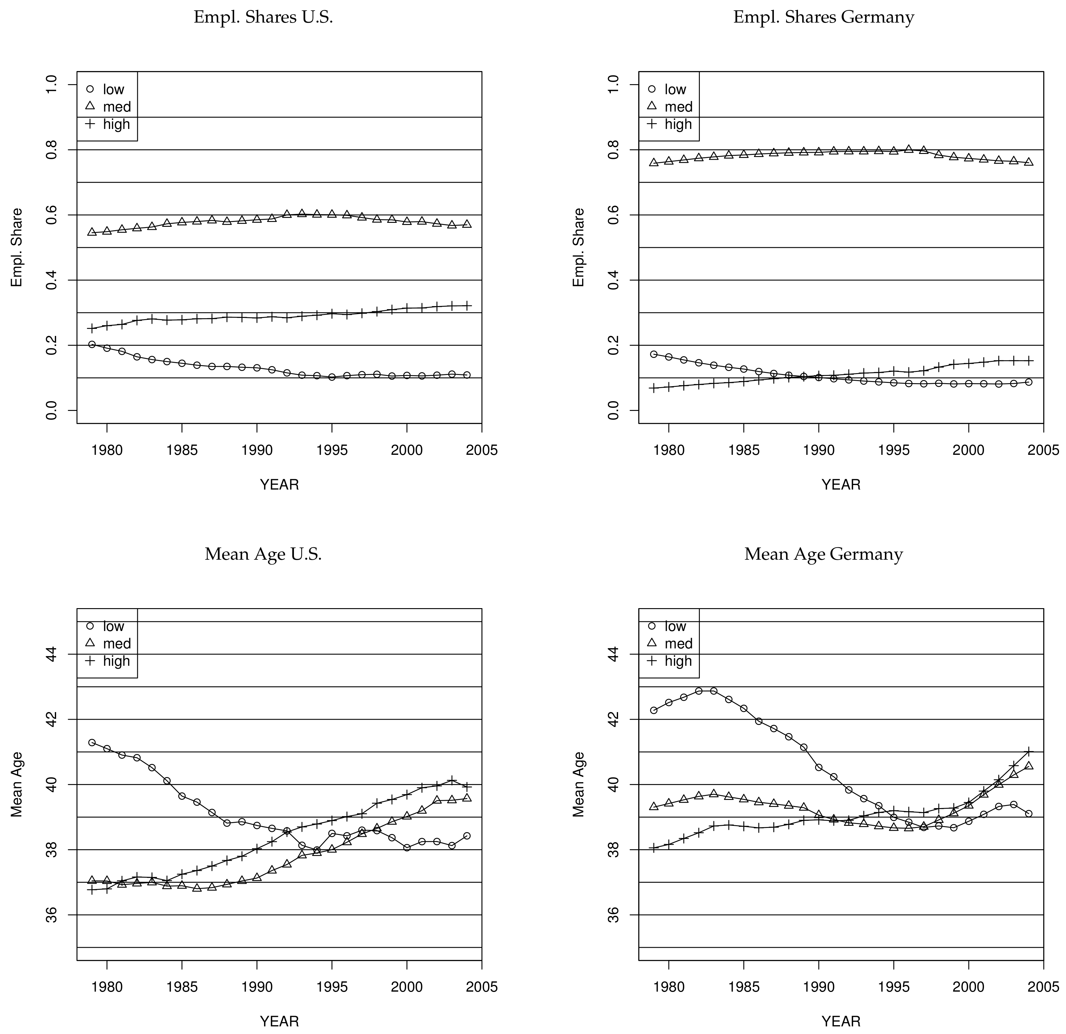
In light of the polarization hypothesis, our choice of education groups was driven by the desire to be able to analysis non-monotonic wage trends/profiles with regard to higher education, i.e., whether the medium-education group is losing ground relative to the high- and low-education groups. If polarization in wages or employment is relevant, the precise definition of the education groups would not matter as long as the medium group covers the middle of the education distribution, which clearly is the case for both countries (see evidence on employment shares in
Figure 1 as discussed in
Section 3.2), even though the size of different education groups differ by country.
2.3. Construction of Cohort-Year-Education Cells
Our level of analysis are wage quantiles by year, cohort/age, and education level, where cohort is defined by year of birth. For each cell, we calculate different quantiles for the real wage. Applying the approach proposed by
Fitzenberger (
1999), this is done for the German data in the following way. The IABS contains information on the social security insurance spells comprising the starting point and the end point as well as the average daily gross wage
12 (excluding employer’s distribution) for this spell.
An annual wage observation for one individual is calculated as the weighted average of the wages he earned during his different spells within one year, where the spell lengths are used as the weights. The sum of the spell lengths for all individuals in one cell is used to calculate the number of employed workers within this cell. This variable is used as a weight in the regressions.
The next step consists of calculating the 20%, 50%, and 80% quantile for the cells, where again the spell lengths are used as weights. We also record the sum of spell lengths as cell weights. In the case of Germany, when the quantile coincides with the threshold, it is recorded as being censored. These information are sufficient for our empirical analysis to estimate quantile regressions based on cell data. The cohort year-skill cell data for the CPS are constructed in an analogous way as for the German data, using the weights described above.
4. Empirical Approach
This section presents the empirical framework developed by
MaCurdy and Mroz (
1995) to investigate the movement of the entire wage distribution for synthetic cohorts over time. A cohort is defined by the year of birth. We estimate various quantile regressions to decompose between- and within-group shifts in the wage distribution. We allow that wage trends differ across cohorts indicating the presence of
cohort effects and across quantiles indicating a trend towards changing within group wage dispersion.
A cohort effect designates a movement of the entire life-cycle wage profile for a given cohort relative to other cohorts. In providing a parsimonious representation of trends in the entire wage distribution, we are able to pin down precisely the differences in wage trends across groups of workers defined by education level.
Due to the inherent identification problem between age, cohort, and time effects, wage profiles based on cross-section relationships between age and wages over a sequence of years and movements of life-cycle wage profiles faced by successive cohorts are mathematically the same mapping. However, considering the wage growth experienced by a particular cohort over time or over age, it can be tested whether apart from the differential age effect, different cohorts exhibit the same time trend.
4.1. Characterization of Wage Profiles
We denote the age of an employee by
and calendar time by
t. A cohort
c can be defined by the year of birth. The variables age, cohort and calendar year are linked by the relation
, which causes the age-period-cohort identification problem. Studies of wage trends often investigate movements of “age-earnings profiles”
The deterministic function
measures the systematic variation in wages (modeling a certain location measure—in our case, conditional quantiles) and
u reflects cyclical or transitory variations. For a fixed year
t, the function
yields the conventional cross-sectional wage profiles. Movements of
f as a function of
t describe how cross-sectional wage profiles shift over time. The cross-sectional relation
f as a function of age does not describe “life-cycle” wage growth for any cohort or, put differently, the cross-sectional relation may very well be the result of “cohort effects”. In fact, “cohort earnings profiles”
given by
represent mathematically the same function as “age-earnings profiles”
, i.e.,
and
represent the same mapping of
to log wages.
The function g describes how age-earnings wage profiles differ across cohorts. Holding age constant, describes the profiles of wages earned by different cohorts over time. Holding the cohort constant yields the profile experienced by a specific cohort over time and age. The latter is referred to as the “life-cycle profile”, because it reflects the wage movements over the life-cycle of a given cohort. Without further assumptions, “pure life-cycle effects” due to aging or “pure cohort effects” cannot be identified, because, e.g., variations in wages due to aging may be associated with changing time based on or changing cohort based on .
4.2. Testing for Uniform Insider Wage Growth
Our analysis investigates whether wage trends are uniform across cohorts in the sense that every cohort experiences the same time trend in wages and the same age-specific wage growth (life-cycle effect). Despite the age-period-cohort identification problem, the existence of a uniform (separable) time trend across cohorts is a testable implication.
The following notion of wage growth proves useful: Wage growth for a given cohort in the labor market over time (“Insider Wage Growth”), given by
comprising the simultaneous change of time and age. Alternatively, holding age constant yields the change of wages earned by different cohorts at specific ages. For the age at labor market entry,
, entry wage growth is given by
again comprising two effects, namely a change of cohort and time. Equation (
4) describes entry wage growth.
If wage growth is separable in age and time, i.e., is the sum of a pure aging effect and a pure time effect as follows
then life-cycle wage growth
is the same for each year
t. Condition (
5) is designated as the “uniform insider wage growth hypothesis” (
). If
holds, we can construct a “life-cycle wage profile” independent of the calendar year and a macroeconomic time trend independent of age. We will investigate
by testing for the significance of interaction terms of
and
t in the specification of
.
Integrating back condition (
5) on the derivative
with respect to
yields an additive form for the systematic component of the wage function
:
where
is the cohort specific constant of integration. At a given point in time, the wages of cohorts differ only by the age-effect, given by
, and by a cohort specific level, given by
. The “uniform insider wage growth hypothesis”
can be tested by investigating whether “interaction terms”
enter specification (
6) which are constructed as integrals of interaction terms of
and
t in
.
4.3. Empirical Implementation
We specify the wage function
for individual
i in the sample year
t using a fairly flexible functional form:
where
and
denote the age of individual
i at time
t and the cohort of individual
i, respectively.
is specified as a smooth function of
c and
. We further decompose the error term into a period specific fixed effect
and a stochastic error term
. In the empirical analysis, we take 25 years to be the age of entry into the labor market and we define
and therefore
. Analogously, since the observation period starts in 1979, we define time
. For each cohort,
c corresponds to the time
t at which
equals zero. For the cohort of age 25 in the year 1979,
c equals zero and older cohorts have negative values for
c.
As a flexible empirical approximation of the wage profile imposing the hypothesis of uniform insider wage growth, we use polynomials in age, cohort, and time:
We include year dummies that are orthogonalized with respect to
to estimate period specific fixed effects
, i.e., the estimated year effects are uncorrelated with the estimated smooth time trend
, see
Fitzenberger and Wunderlich (
2002) for details. Altogether, we fully saturate the time dimension, i.e., the model is estimated as if a complete set of year dummies is used. However,
is estimated just as if no further year effects
where included. Thus,
represents the year specific deviation from the smooth trend
, which we interpret as cyclical year effect. We estimate a fifth order polynomial in time for
, yielding a satisfactory decomposition of trend and cycle.
14 Equation (
8) allows for a third order polynomial in age, a third order polynomial in
, and a second order polynomial in
.
15To test
, we consider in the derivative
the following four interaction terms of age and time
,
,
, and
. The implied non-separable variant of
expands (
6) by incorporating the integrals of these interaction terms, denoted by
-
, see
MaCurdy and Mroz (
1995) and
Fitzenberger and Wunderlich (
2002) for details, and we test for significance of
-
.
16Only if
holds, it is meaningful to construct an index of a life-cycle wage profile as a function of pure aging
a macroeconomic trend index. Otherwise, a different wage profile would apply for each cohort. Under
, the life-cycle
is given by
and the macroeconomic
wage trend index is given by
When interpreting these indices, it is important to recognize that neither the level nor the coefficient on the linear term are identified in an econometric sense. In fact, identification relies on the assumption that the coefficient on the linear cohort term is equal to zero. To motivate this, we argue that setting the linear cohort term to zero is quite natural. If, for instance, also entry wages grow at the same rate as the time effect before and during the sample period, the entire cross-section profile exhibits purely parallel shifts over time, a situation, one would not naturally characterize by the existence of “cohort effects”. Our notion of a cohort effect requires a situation where the differences in starting points of the common life-cycle profile differ from the macroeconomic wage growth experienced by the cohorts in the labor market. For this reason, we also orthogonalize our polynomial specifications for and with respect to the linear cohort effect.
Quantile regressions provide a useful tool to study wage differences across and within groups of workers with different socio-economic characteristics. We estimate conditional quantiles of wages
where
denotes the
-quantile of the wage in cohort age-cell
(≡ cohort year-cell
where
). The vector
comprises the coefficients relating to the set of regressors (≡ powers of
and
t; year dummies). In the empirical analysis, we model the following quantiles:
(20%, 50%, and 80% quantile).
We use the minimum-distance approach proposed by
Chamberlain (
1994) or
MaCurdy and Mroz (
1995) for the estimation of quantile regressions when the data on the regressors can be grouped into cells and censoring is not too severe. The approach consists of calculating the respective cell quantiles in a first stage and regressing (by weighted least squares) those empirical quantiles, which are not censored, on the set of regressors in the second stage. For the dataset used in this study, the cell sizes are large enough for making this a fruitful approach. However, for Germany, we do not estimate the 80% quantile for males in education group (H) since censoring is too severe in this case. When applying the minimum-distance approach, we use the cell sizes as weights.
The error terms are allowed to be dependent across individuals within cohort year-cells and across adjacent cohort year-cells. We use a flexible moving block bootstrap approach allowing for standard error estimates which are robust against fairly arbitrary heteroscedasticity and autocorrelation of the error term. The block bootstrap approach employed here extends the standard bootstrap procedure in that it draws blocks of cell observations, including the cell weights, to form the resamples. While the goal to capture dependence across observations is similar to a cluster bootstrap, we do not rely on fixed cluster but rather moving clusters which overlap. Specifically, we draw a two-dimensional block of observations with block length eight in the cohort and block length six in the time dimension with replacement until the resample has become at least as large as the resample size, see
Fitzenberger and Wunderlich (
2002) for details. Contrasting the results using the moving-blocks-bootstrap approach with conventional standard error estimates indicates that allowing for correlation between the error terms within and across cohort year-cells (when forming the blocks) changes the estimated standard errors considerably (detailed results are available upon request).
5. Results
Based on the empirical framework introduced above, this section discusses the estimated specifications and then presents the empirical results.
5.1. Estimated Specifications for Wage Equations
We estimate two specifications for the 20%, 50%, and 80% quantile for males by education groups (U), (M), and (H). The high degree of censoring allows only a meaningful estimation of the more restrictive specification for the 20% and the 50% quantile in the case of high-education (H) males in Germany.
The more general specification (Model 1), which does not impose the uniform insider wage growth hypothesis (
) introduced in
Section 4.2, is given by
where the age polynomial is of order 3, the time polynomial of order 5, and
and
are the cohort terms before and after 1979, orthogonalized with respect to the linear cohort term. All specifications include the cyclical year dummies
which are orthogonalized with respect to the time trend, thus
(we lose six degrees of freedom [
] because an intercept is included).
Model 2 is the restricted version of Model 1 in Equation (
12):
Model 2 imposes
, i.e., separability of wage growth into age and time effects. Statistical tests imply that for all education groups at the three quantiles considered both life-cycle profiles [Equation (
9)] and macro-trends [Equation (
10)] are the same across cohorts, because
cannot be rejected at a 1% significance levels (detailed results are available in the
Supplementary Material, Tables S1 and S2). In all cases except two, we also do not find significance at the 5% significance level. Note that we do not perform the test for high-education workers in Germany because of the high degree of censoring in this group (see
Section 2). Because of the evidence in favor of
, we only report in the following estimation results for Model 2. For this model, the estimation of time trends and life-cycle profiles is thus meaningful. Even though, further hypothesis tests would suggest to use a more parsimonious specification of model (see again
Tables S1 and S2 in the Supplementary Material), we do not further restrict the model specifications because we do not want to base the comparison across worker groups on differences in specification choices. We also include estimates of Model 2 for high-education workers in Germany for the 20%- and the 50%-quantile.
5.2. Life-Cycle Profiles
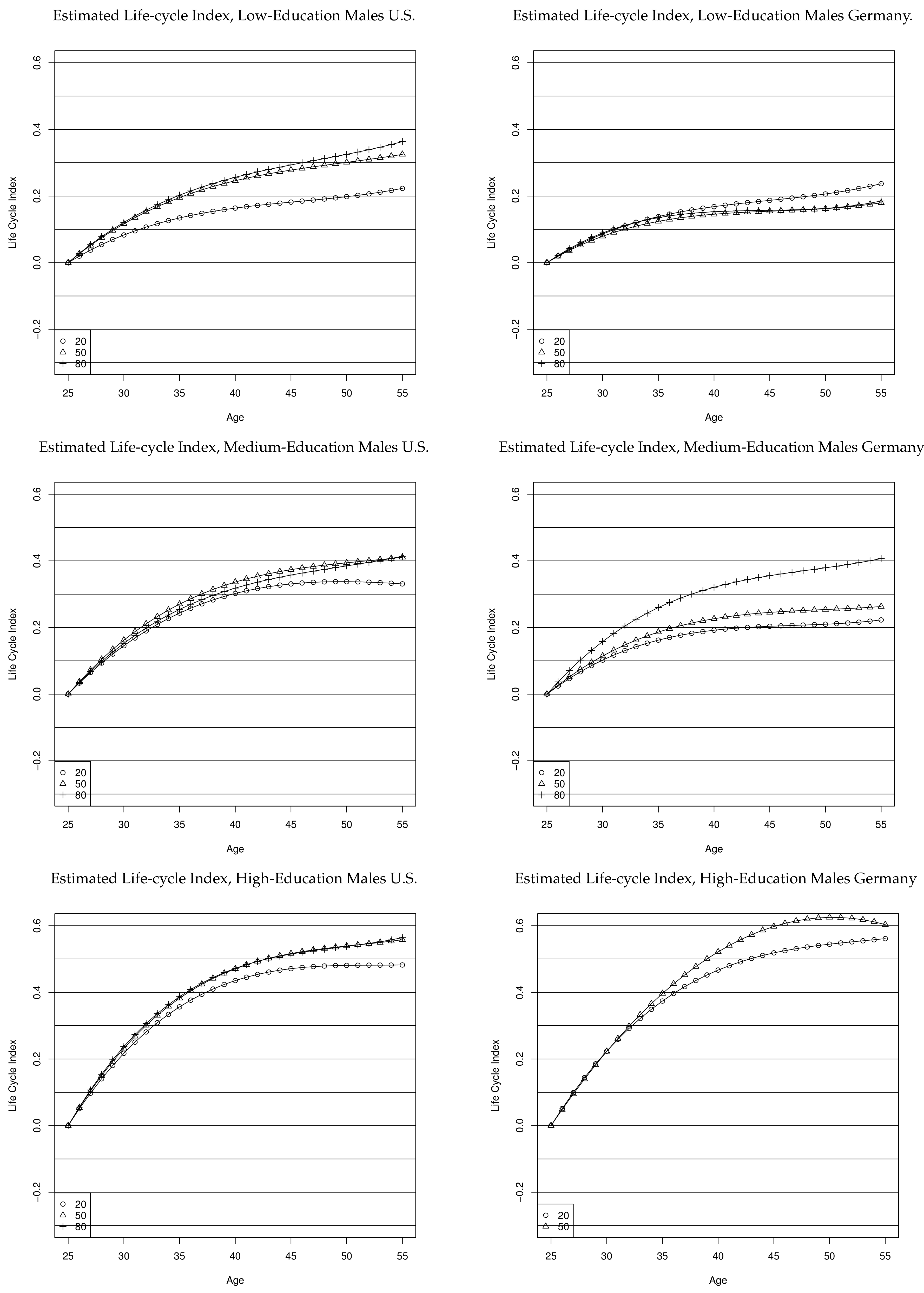
Figure 6 shows the estimated life-cycle profiles. Note that wage growth over the life-cycle at the median wage, which closely relates to a standard human capital wage equation (
Gosling et al. 2000), is positively correlated with educational level—i.e., the descriptive returns to experience are increasing with education. For most cases, life-cycle wage growth is higher at higher quantiles (and mostly significantly so, detailed results are available upon request), i.e., inequality within education group typically increases with age. There are three exceptions: At the 50% and 80% quantile for medium-education in the U.S. and for low-education in Germany, life-cycle profiles basically coincide which implies that upper-tail wage dispersion does not increase with age. For low-education in Germany, life-cycle wage growth is even higher at the 20% quantile than at the median, i.e., for this education group lower-tail wage dispersion falls with age.
Despite the similar concave profiles, the amount of within-cohort life cycle wage growth differs both across education groups and across countries. Life-cycle wage growth increases with education in both countries and is higher in the U.S. for low-education at the two higher quantiles and for medium-education at the two lower quantiles. Life-cycle wage growth is very similar in both countries at the upper quantile for medium education and at the two lower quantiles for high education.
The decreasing within-cohort wage dispersion when workers age for low-education in Germany may be due to a selection process. Older German low-education workers at the bottom of the skill-specific wage distribution might drop out of the labor-market as they get older, e.g., due to layoffs, if their productivity lies below the wages set by union wage agreements. Contrary to low education, the increase of within-cohort wage dispersion associated with aging is twice as strong for German medium-education workers compared to U.S. medium-education workers. This may reflect the larger heterogeneity of the medium education group in Germany, which comprises a higher share of workers compared to the medium education group in the U.S.
The development of wage dispersion over the life-cycle for the U.S. is in line with findings for the UK (
Gosling et al. 2000). Wage dispersion over the life-cycle grows less for higher education levels, i.e., in the U.S. low-education workers experience the highest increase in wage dispersion over the life-cycle, while for Germany dispersion increases most strongly for medium-education in the upper part of the wage distribution.
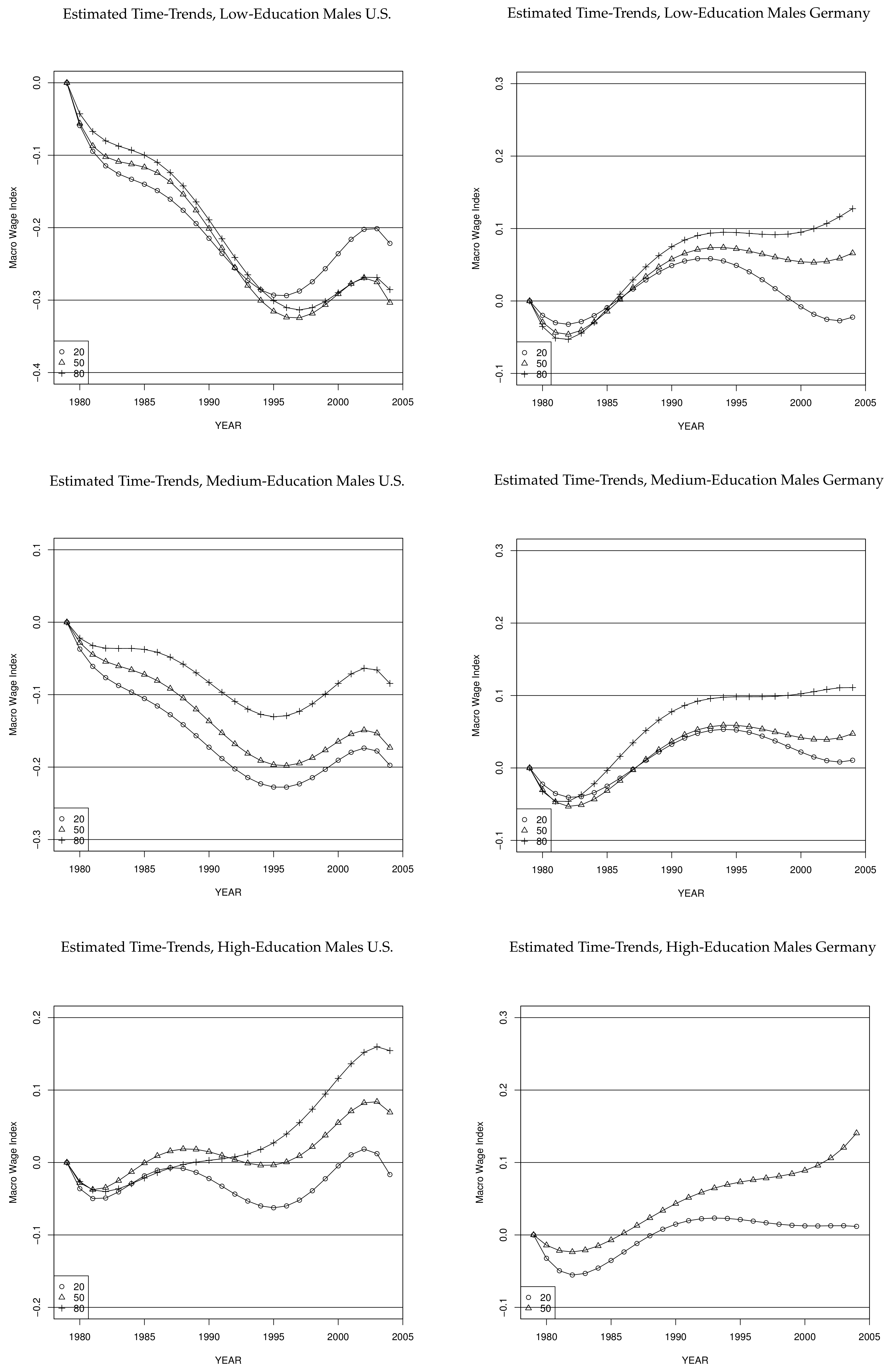
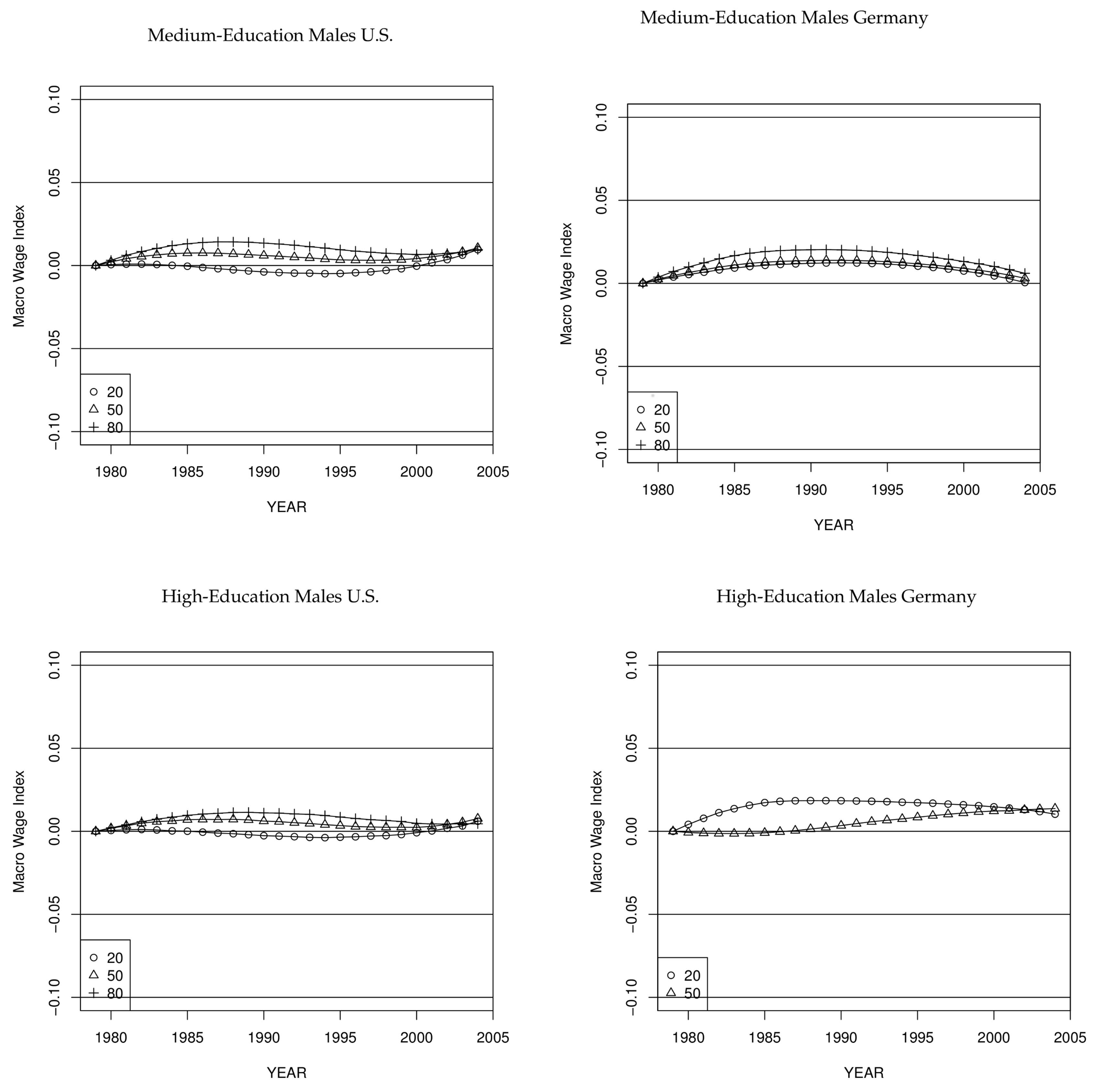
5.3. Time-Trends
Figure 7 depicts trends in real wages due to macroeconomic shifts in the U.S. and Germany. Time-trends in the U.S. were more positive for workers with higher educational attainment than for low- and medium-education workers. Comparing low- and medium-education workers in Germany at the different quantiles, we see that time-trends in wages were roughly the same across education groups. Time-trends for German high-education workers were similar to those of less skilled workers until the early 1990s, but wage growth was stronger thereafter. Finally, our estimates suggest that time-trends in wages developed more positively for German workers than for U.S. workers.
The mid-1990s mark a turning point in the development of the macro wage indices of both low-education and medium-education worker in the U.S. Until that point in time, workers in both subgroups experienced real wage losses throughout the entire wage distribution, being stronger for the low-education (−30 log points at the 80% and 20% quantile and −32 log points at the median). Medium-education workers incurred losses of −11, −20, and −22 log points at the 80%, 50%, and 20% quantile, respectively. Between 1996 and 2004, however, wages grew considerably at all considered quantiles of both low- and medium-education workers. Wages for low-education at the 20% quantile grew by 10 log points, wages at the median and at the 80% quantile by 5 log points. For medium-education, the wage growth starting in the mid-1990s was less pronounced. Wage growth was about 4 log points at both the 20% and the 80% quantile and about 3 log points at the median. Time trends are most positive for high-education workers in the U.S., with a cumulated wage growth of −1, 8, and 17 log points at the 20%, 50%, and 80% quantile, respectively, between 1979 and 2004.
For low-education workers in Germany, the 20%, 50%, and 80% quantiles of the wage distribution move in a parallel manner between 1979 and 1992, resulting in an uniform gain of about 8 log points along the entire distribution. Thereafter, wages at the 80% quantile exhibit small gains, while the wages at the 20% quantile decrease, resulting in real wage losses of 5 log points between 1992 and 2004. Wages at the median remain flat during this period.
17 Medium-education workers in Germany do slightly better than low-education workers, in terms of time-trends at the lower end of the skill-specific wage-distribution. Time-trends for wages at and above the median are fairly similar. Cumulated wage growth at the 20% quantile for German medium-education workers is slightly above zero, compared to real wage losses of about 2 log points in the group of the low-education. However, this masks the fact that since the beginning of the 1990s, real wage losses are more pronounced among low-education workers in the lower part of the distribution. Wages at the 20% quantile of German high-education workers were staying flat since the beginning of the 1990s. Over the entire period, cumulated wage growth is about 1 log points for this group at the 20% quantile. The time-trend for German high-education workers at the median starts to increase monotonically in the early 1980s, at an annual rate of about 0.5 log points. Wages at the 20% quantile were rising between the early 1980s and the early 1990s, but then started to flatten out.
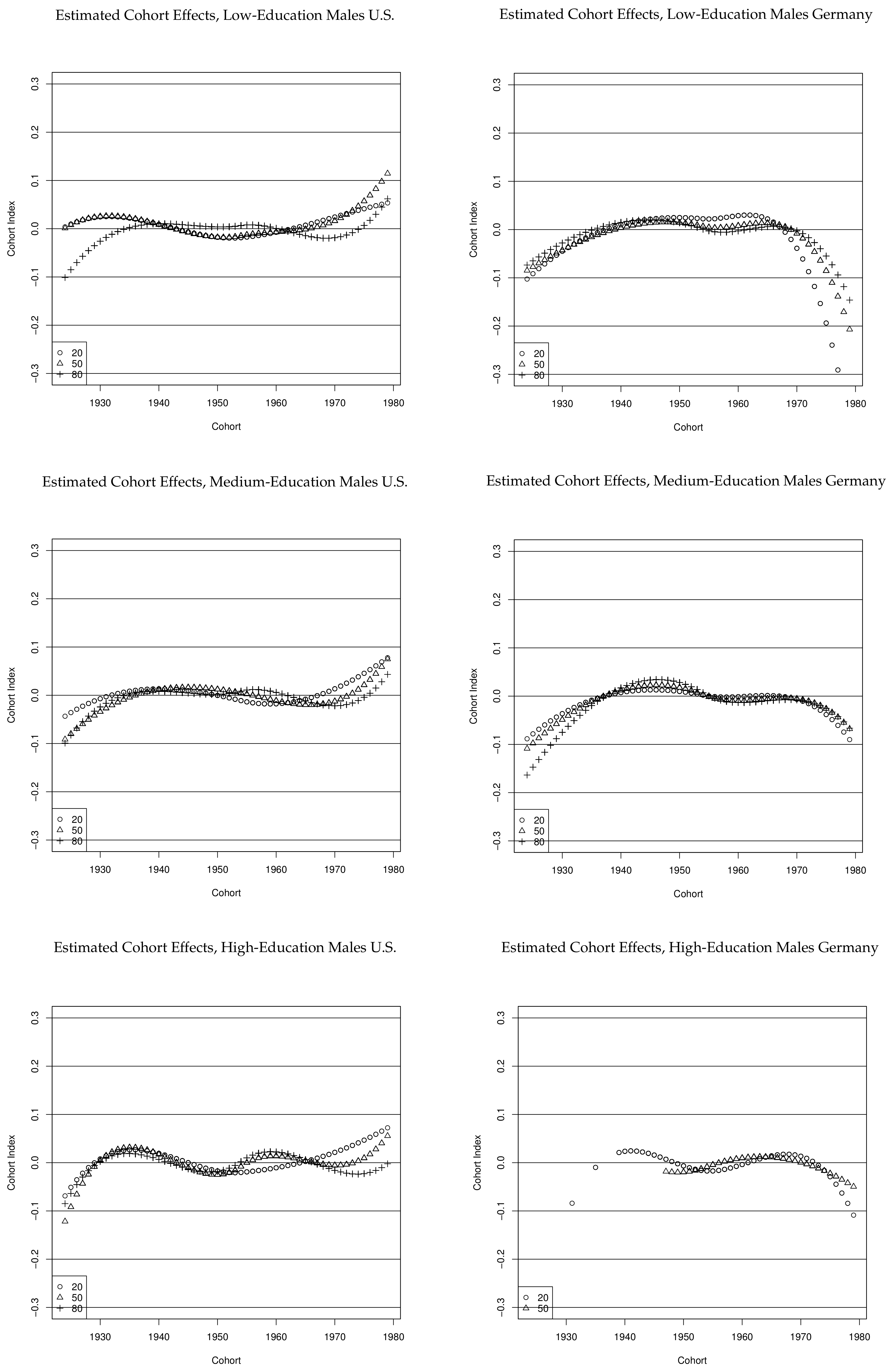
5.4. Cohort Effects
There are a number of reasons for the existence of cohort effects. Not being exhaustive, we discuss three. First,
Card and Lemieux (
2001) argued that the increasing wage premium between college graduates and high-school graduates is due to a slowdown in the growth of supply of higher-skilled workers. Second, cohort effects may reflect changes in educational policy, or more generally, any pre-labor market conditions (
Carneiro and Lee 2011). Third, cohort effects may reflect labor market conditions at labor market entry which may have lasting effects over the life course (see, e.g.,
Berger (
1985) for the effect of cohort size). In a labor market with frictions, cohort effects may be implied by wage adjustments which are strongest among younger workers at labor market entry and which may persist over the life cycle. These mechanisms may operate at the same time and our analysis will not be able to distinguish between them.
Figure 8 plots the estimated cohort effects for the different groups in both economies. These are quadratic and cubic terms for cohorts that enter the labor market before and after 1979, orthogonalized to the linear cohort term. For both medium- and high-education workers in the U.S., negative cohort effects are estimated for the oldest cohorts and positive effects for the youngest cohorts. For low-education workers, we find positive cohort effects for the youngest cohorts and negative ones for the oldest cohorts at the 80% quantile. Interestingly, we find that during the 1980s cohort effects had a positive effect on medium-education and high-education workers—this is the period for which
Card and Lemieux (
2001) observed increasing skill premia among younger workers for the U.S.
18 For Germany, for all education groups, both the youngest and the oldest cohorts exhibit negative cohort effects, relative to the cohorts entering the labor market between the mid-1960s and mid-1980.
19 Furthermore, the youngest cohorts experience higher within-cohort wage dispersion due to these effects.
The trend in entry wages is the sum of cohort effects and the macroeconomic time-trend (see
Section 4;
Figure S1 in the Supplementary Material shows the estimated entry wages over time). In the U.S., positive cohort effects for the youngest cohorts partly reverse the decline in real wages for low- and medium education. Furthermore, entry-wages become more dispersed among medium- and high-education workers, and less dispersed for low-education workers. In Germany, the negative cohort effects and the increase in within-group wage dispersion for younger cohorts since the 1990s add to the rising wage dispersion, especially within education groups. The least-paid low-educated workers show the largest real wage loss at labor market entry. While cohort effects mitigate within-group inequality of entry wages in the U.S. cohort effects are more sizeable the low-educated in Germany and strongly increase inequality of entry wages, especially in the lower tail of the wage distribution.
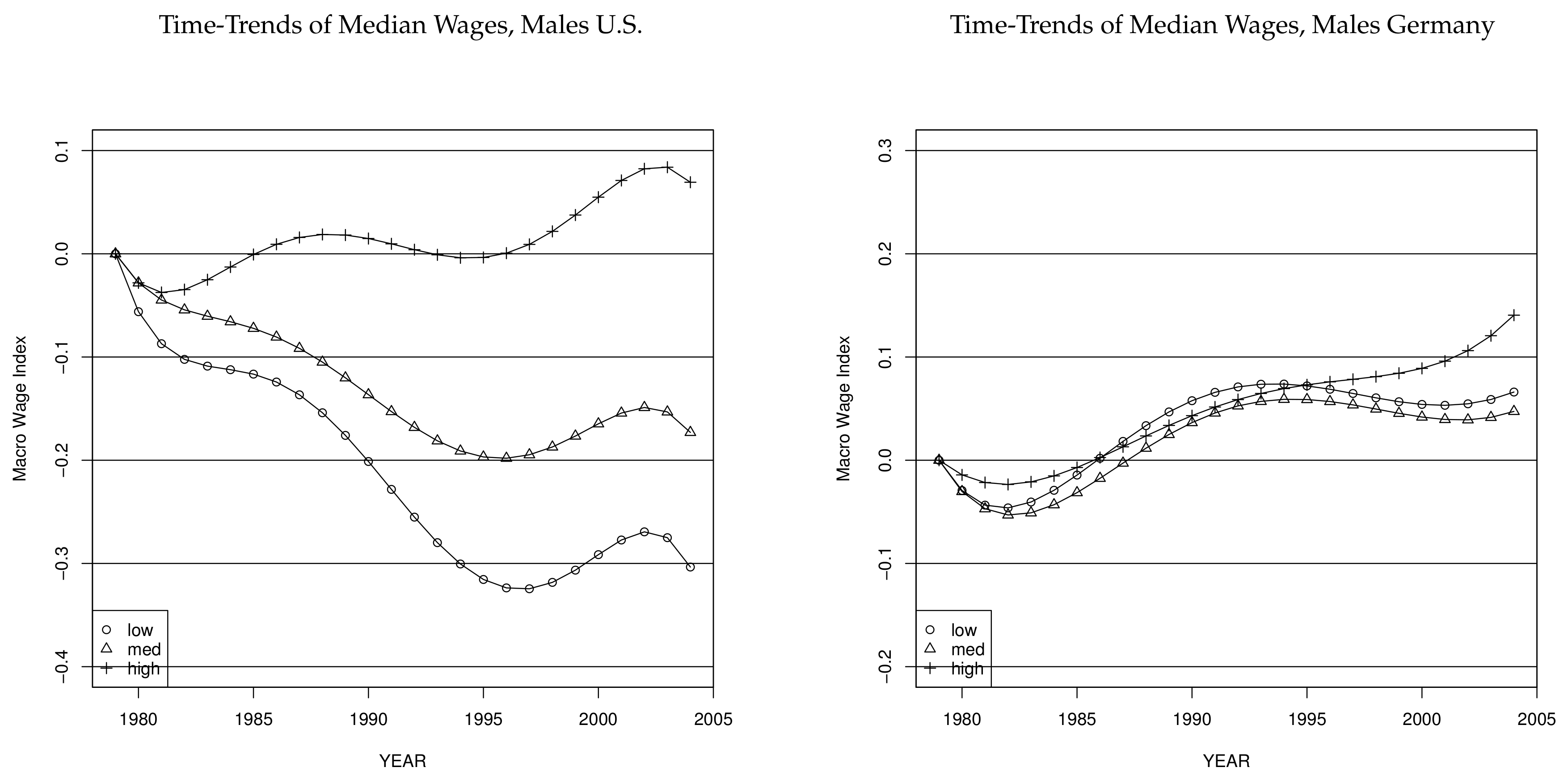
5.5. Uniformly Rising Wage Dispersion or Wage Polarization?
5.5.1. Development of Skill Premia due to Macroeconomic Shifts
How much of the increase in wage dispersion in the U.S. and Germany is due to rising skill premia across educational groups? Some studies have suggested that this part is substantial. For example,
Lemieux (
2006b) found that almost half of the increase in wage inequality in the U.S. can be explained by changes in skill premia. For Germany, our descriptive results in
Section 3 show that the rise of the low-to-medium education premium and the increase in dispersion in the lower part of the German wage distribution in the 1990s take place during the same period. Most of the rise of the education premium between high- and medium-education workers occurs also after 1990.
Figure 9 depicts the estimated time-trends of median wages across education groups. Cumulated wage growth over time in the U.S. at the median is much better the higher the education level, i.e., the education premium is increasing strongly which is consistent with the SBTC. Note, however, that the medium-to-low wage premium started to decrease slightly since the mid-1990s, which reflects a weak (albeit not significant) tendency towards wage polarization (see
Autor and Dorn 2013;
Autor et al. 2008) for further evidence of wage polarization during the 1990s in the U.S.). For Germany, until the mid-1990s, median-wages across education groups move in a parallel fashion. Since then, wages of the high-education exhibit higher growth rates than those of low- and medium-education workers, while the education premium across medium- and low-education German workers does not change over time. The latter observation is somewhat surprising, as the unconditional dispersion between those two groups at the median is clearly increasing since the end of the 1980s (see
Figure 5). What can explain these differences between the unconditional development of the education premium and the time-trends? Below, we provide evidence that negative cohort effects for young low-education workers have contributed to the increasing education premium observed unconditionally
20— which could have been caused by the inflow of young low-education workers into West Germany after the fall of the iron curtain (note that
D’Amuri et al. (
2010) and
Glitz and Wissmann (
2017) provided evidence against this). Moreover, and at least as important, we find that the decline in average age of low-education workers and changes in the age-structure of the group of the medium-education (
Figure 1) contributed to the rising education premium in Germany, as
Figure 10 reveals. Mechanically, this happens because the median wage of the medium-education (low-education) workers increases (decreases) as medium-education (low-education) workers become older (younger). Finally, unions may have successfully counteracted an increasing education premium between medium- and low-education workers, which otherwise would have prevailed due to technological change. The same mechanical compositional effects account for roughly 40% of the sharp increase of 17 log points in the education premium between medium- and high-education workers in Germany during the early 1990s and 2004, which is observed unconditionally. During the early 1980s, time-trends seem to play no substantial role in explaining the somewhat increasing education premium between medium- and high-education German workers observed unconditionally.
For the U.S., the time-trends describe the same qualitative but attenuated patterns for the skill premia as the ones observed unconditionally. During the 1980s, when the education premium between medium- and low-education U.S. workers increased, negative cohort effects for the low-education were at work. The declining age of low-education workers also contributed to the rising wage premium, while the age-structure of medium-education workers was quite stable during the 1980s. Regarding the wage premium between high-education and medium-education in the U.S., we see that the aging of the high-education contributed to an increasing premium during the 1980s. Altogether, we find somewhat similar patterns regarding the compositional effects on the wage premia for the U.S. and Germany.
Macroeconomic shifts are likely to be smooth functions of SBTC, institutional factors,
21 and supply-side factors. Given that we observe two industrialized countries that arguably have access to the same technologies, our evidence regarding the different developments of education premia is unlikely to be explained by technological change alone. In fact, supply-side and institutional factors seem to play a key role in explaining the rise of unconditional wage differences between education groups in Germany. This suggests to consider the interaction between labor market institutions, supply-side effects, and SBTC.
22 Note that trends in relative labor-supply across education groups as well as the age-pattern within skill groups show very similar trends in both countries. This indicates that institutional factors—and their interaction with SBTC—may be more important than supply-side factors in explaining the differences across countries.
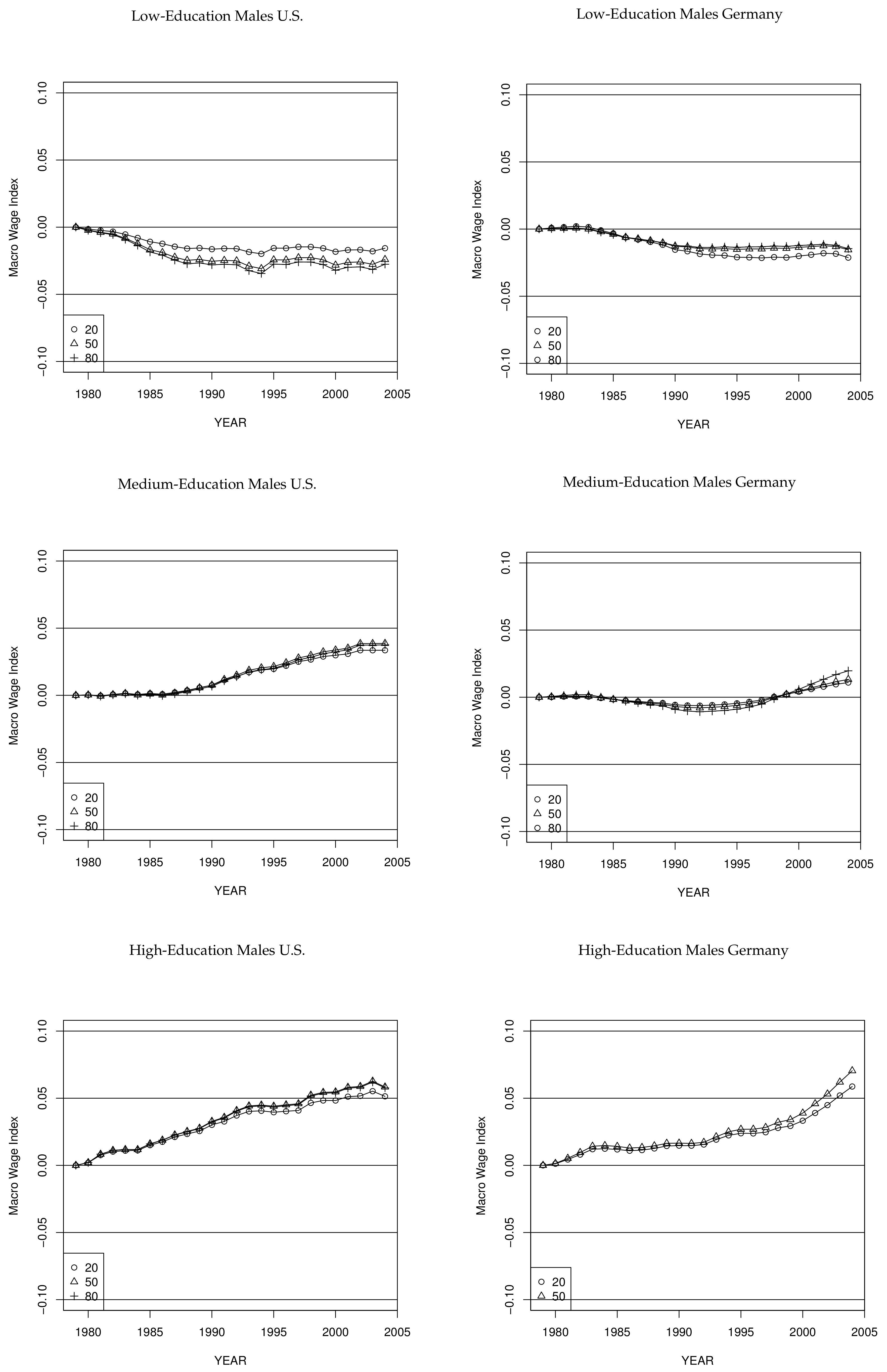
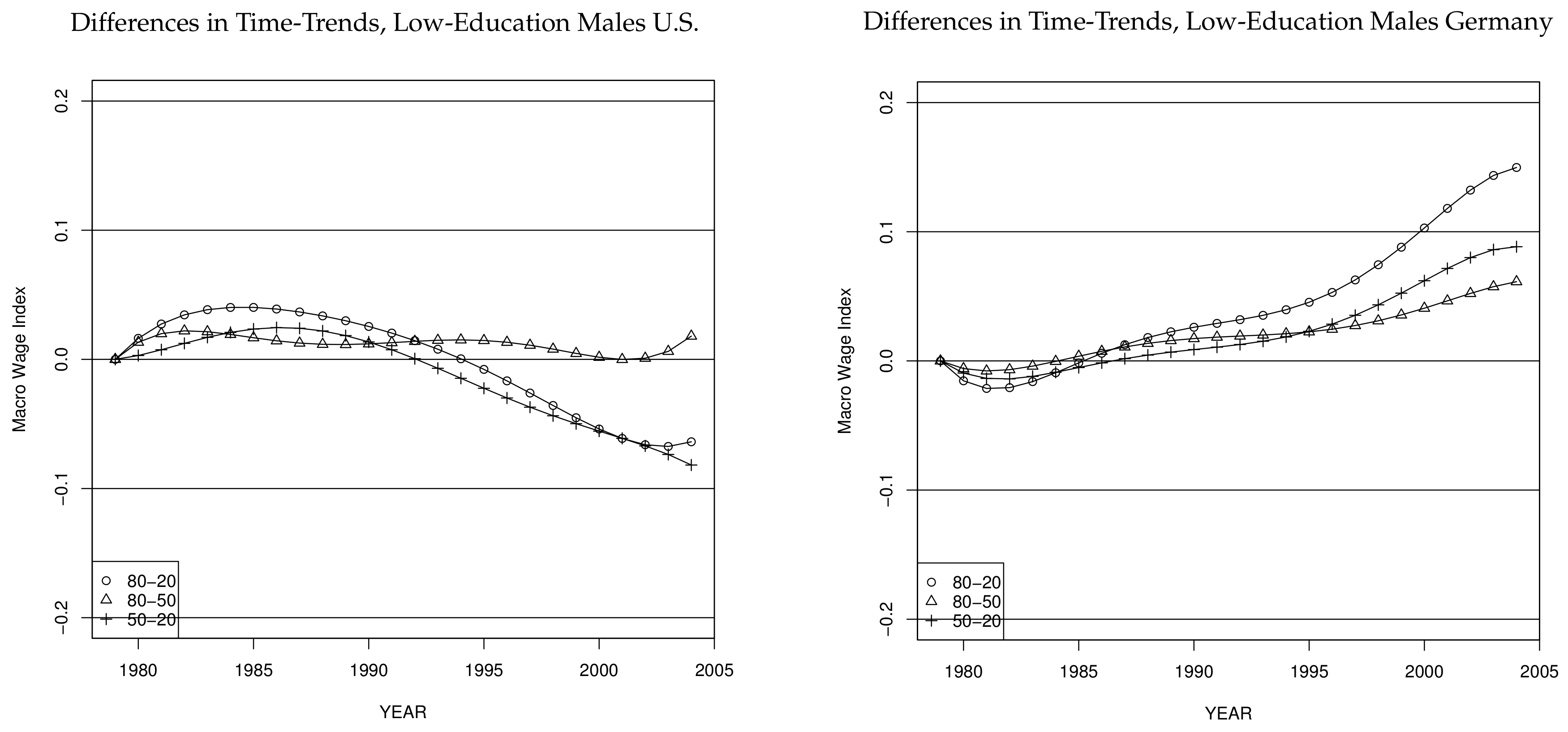
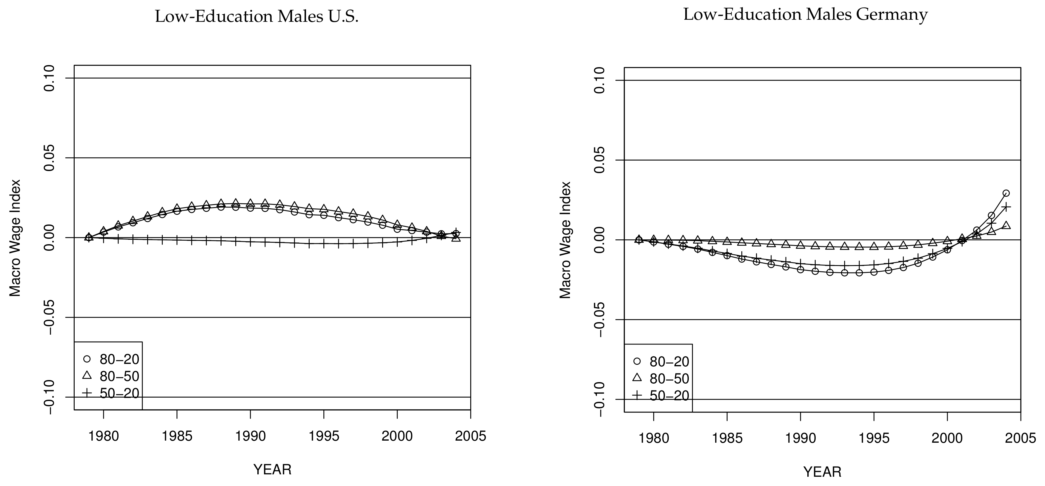
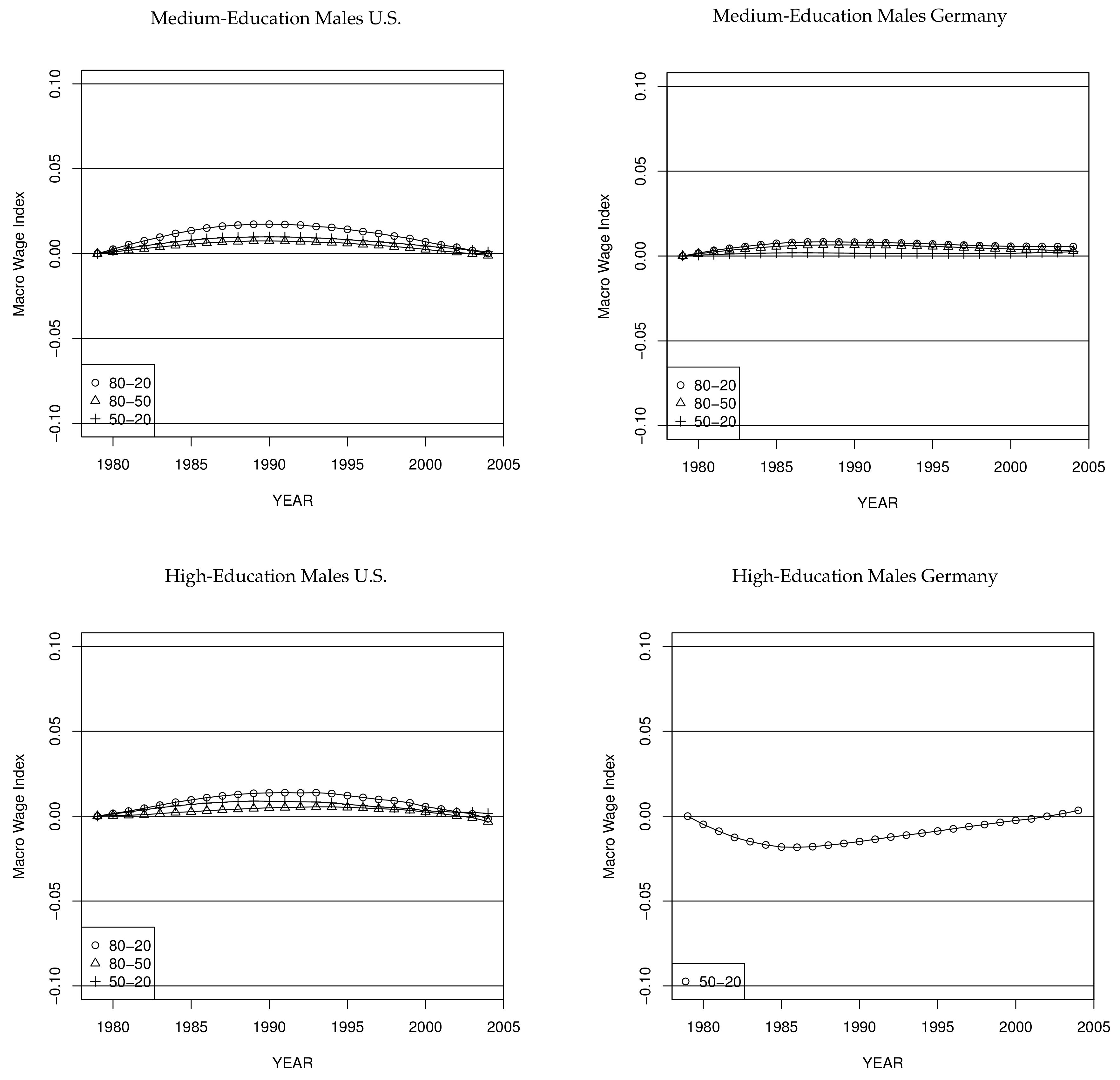
5.5.2. Wage Dispersion within Skill-Groups
Since the macroeconomic changes in education premia are very small in Germany, most of the increase of wage dispersion in Germany is therefore likely to be due to diverging time-trends within education groups. For low-education workers,
Figure 11 depicts the estimated macroeconomic changes in within-group inequality due to macroeconomic shifts within education groups, as measured by the difference of the time trends at the three quantiles. We focus on the strong differences across countries found for low-education workers. The trends for medium- and high-education are fairly similar across countries generally showing a similar increase in within-group wage dispersion over time (see
Figure 7 in the main text as well as
Figure S2 in the Supplementary Material).
In the U.S., low-education workers experienced an astonishing decline in wage dispersion in the lower part of the wage distribution starting in the mid-1980s. After a short period with a rise of the 50%–20% difference by 2 log points, wages at the median dropped more sharply then wages at the 20% quantile until 1996 (and thereafter increased more slowly), resulting in a decreasing dispersion of the lower part of the wage-distribution. Moreover, this decrease is the driving force behind the decline of overall decreasing wage inequality, as measured by the 80%–20% difference, as the inequality in the upper part was quite stable between 1980 and the end of the 1990s (thereafter wage inequality in the upper part decreased by about 2 log points).
23 Increasing wage inequality among U.S. medium-education workers since the early 1990s masks a weak polarization pattern which starts as early as the end of the 1980s, because from then onwards wage growth is slightly higher at the 20% quantile compared to the median. Inequality increases above the median during the 1980s and afterwards basically stays constant.
Our results regarding wage inequality of U.S. low-education workers and the lower part of U.S. medium-education workers for the 1980s may reflect “episodic events”, such as the declining real minimum wage and deunionization, and are thus in line with
Card and DiNardo (
2002).
24 The polarization of wages, beginning at the end of the 1980s, has also been documented by
Autor and Dorn (
2013), who argued that the low-skill service sector is the driving force.
The highest increase of overall wage dispersion, as well as dispersion in the lower part of the distribution, is observed for the group of high-education workers in the U.S. for whom neither unions nor minimum wages are likely to play an important role. It is rather likely that technological change had heterogeneous effects among the group of college-graduates (see
Lemieux 2006b). Moreover, changes in social norms might have played a certain role especially for this group (see
Piketty and Saez 2003).
After a short period of decreasing overall wage inequality in Germany between 1979 and 1982, low-education workers experience a large increase in wage dispersion, where the rise in the 50%–20% difference dominates after the mid-1990s. Unemployment rates in Germany are high among those workers, hence there might also be selection processes driving these developments.
Until the mid-1990s, the 50%–20% difference of medium-education workers in Germany remained almost unchanged, compared to 1979. The rise in overall wage inequality until then was purely driven by an increasing dispersion in the upper part of the wage distribution. Since the mid-1990s wage dispersion is increasing monotonically both in the lower- and upper part of the distribution (this is similar to findings in
Dustmann et al. (
2009)).
The 50%–20% difference of high-education workers is quite flat until the early 1990s, when it starts to increase monotonically until the end of our observed period. The late increase in wage dispersion among German high-education workers is interesting considering the fact that unconditional wage dispersion in Germany at the top already started to increase during the 1980s. Apparently this was not caused by an increasing within-wage dispersion among high-education workers below the median.
What explains these differences in the development of polarization between the U.S. and Germany? For the U.S., we see patterns of polarization due to macroeconomic shifts both within and across education groups.
25 For Germany, we find little evidence after the early 1980s for polarization of unconditional wages and of wage inequality within education groups.
Similar to
Fitzenberger and Wunderlich (
2002) and
Dustmann et al. (
2009), the development of the German wage structure is consistent with the SBTC story, if one allows for institutional factors (including the effects of social norms
Piketty and Saez (
2003)), such as unions and implicit minimum wages implied by the welfare state, which, in comparison to the U.S., delayed the widening of the German wage dispersion in the lower part for about ten years. A further explanation might be that social norms in Germany have been different, an explanation which is put forward by
Piketty and Saez (
2003) for other continental European countries as well. Similar to the argument made by
Chernozhukov et al. (
2013) that the decline of unions and of the minimum wage in the 1980s in the U.S. counteracted the polarization of wages during that period, the increasing flexibility in Germany due to a higher decentralization of wage setting during the 1990s and the early 2000s (see
Dustmann et al. 2014) may have counteracted a polarization of wages.
5.5.3. Compositional Effects on Wage growth and Inequality
Figure 6 depicts the life-cycle profiles of wage growth conditional on education, showing that inequality varies by age. To illustrate this,
Figure 10 plots the effect of the changing age structure on wage growth and (implicitly) on wage dispersion. This is done by using the estimates of the life-cycle profile of wages and the changing distribution of ages to calculate the implied change in wages. The increase of the mean ages both of medium- and high-education workers in the U.S. reflect the changes of the age structure which result in increasing wages in these two subgroups. However, wage inequality within education groups only slightly increases due to the changing age structure. The trend for low-education workers in the U.S. is reversed: The mean age decreases between 1979 and 2004, and changes in the age-structure lead to decreasing wages as well as less wage-inequality over time, being mainly driven by declining wage dispersion in the lower part of the wage distribution. Comparing the development of the wages at the medians across education groups, it is clear that, first, throughout the entire period the changing age structure among low- and medium-education U.S. workers led to an increasing education premium between medium and low, second, that during the 1980s, the aging of high-education workers led to an increasing education premium between high and medium.
For Germany, the results differ for the low-education. Although the age-pattern is qualitatively the same between 1979 and 2004 compared to the U.S., the rejuvenation of this education group, indicated by a decrease of the mean age, leads to an increasing within wage dispersion over time, as the 20% quantile in this group experiences the largest life-cycle wage growth. The changing age-structure of medium- and high-education workers in Germany, indicated by the rise of the mean age starting in the late 1990s, mechanically leads to increasing wages for both groups. The age-decomposition effect only plays a minor role in explaining changes of wage dispersion conditional on education though. The aging of German medium-education workers since the early 1990s led to an increasing education premium between low- and medium-education workers, which, as we have shown above, is not due to macro-economic shifts. Similarly, differences in the pattern of aging between medium- and high-education workers led to an increasing education premium between those two groups.
Figure 12 and
Figure 13 depict the impact of the inflow and outflow of the cohorts on skill-specific wage growth and dispersion, respectively. The latter graphs show that starting in the early 1990s, the change in the cohort structure supports the catching-up process of both wages at the median and the 20% quantile to wages at the 80% quantile in the group of low-education workers in the U.S. The 80–50 and 80–20 difference of wages had increased before, though, due to cohort effects. Contrary to that, cohort effects in Germany for the group of low-education led to an increasing wage dispersion of about 5 log points throughout the entire wage-distribution between 1992 and 2004, while before the early 1990s, cohort effects led to a decreasing wage dispersion, with the movements of the 80-20 difference mainly being driven by changes of the wage dispersion in the lower part. Cohort effects for medium- and high-education workers affect wage dispersion somewhat less in both countries. Relatively to the oldest and the youngest cohorts, those in the middle seem to exhibit higher cohort specific wage dispersion, driven mostly by positive cohort effects at the median and the 80% quantile. In the middle of the observation period, the presence of these cohorts in the middle is strongest, resulting in the strongest increase in wage dispersion within skill groups. Based on
Figure 12, the sharp drop of cohort effects among low-education German workers mechanically increases the wage premium between low- and medium-education workers in Germany. Compositional effects regarding the cohort structure also seem to increase the education premium between high- and medium-education workers in Germany since the early 1990s. For the U.S., such compositional effects play only a minor role.
5.6. Employment Growth
A large literature finds polarization of employment in both Germany and the U.S. since the 1980s based on employment trends for occupations (see, e.g.,
Autor et al. 2003;
Spitz-Oener 2006). We complement these findings based on data for age-education cells. Using a method similar to
Card et al. (
1999), we rank the age-education cells across education groups for a base year according to the cells unconditional median wages, which we normalized by the estimated age-specific life-cycle wage growth of the specific cells, i.e., we do not use the unconditional wage level as in the polarization literature (e.g.,
Autor and Dorn 2013).
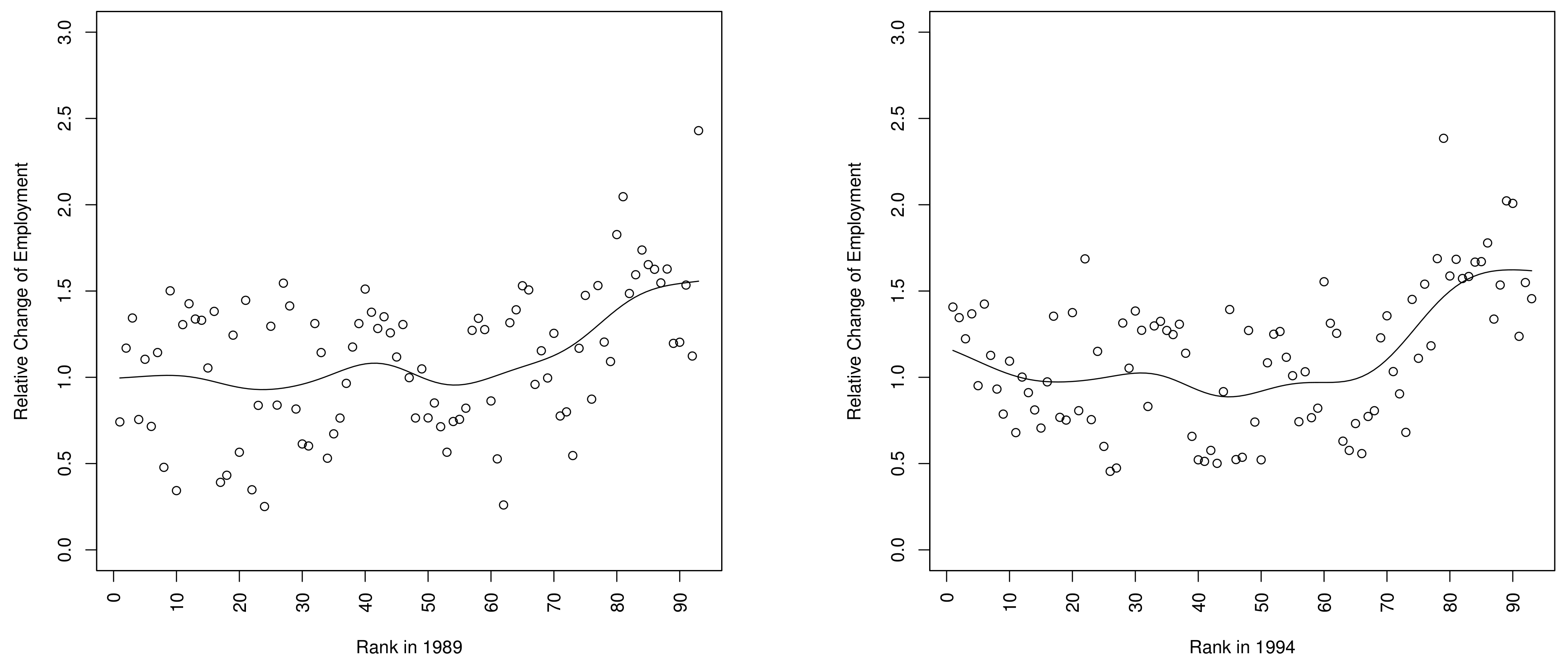
26 Then, we calculate the cumulated relative employment growth of each cell over the next ten years.
27 Our age variable is discrete, ranging between 25 and 55, and we distinguish between three educational levels, which yields 93 cells for this analysis, which
Card et al. (
1999) interpreted as “education groups”. The base years we choose are 1979, 1984, 1989, and 1999. The results are depicted in
Figure 14 and
Figure 15.
For the base years 1979 and 1984, relative changes in employment in both economies is a monotonically increasing function of the rank of wages in the base year. We find evidence of employment polarization in Germany starting with the base year 1989, which becomes more pronounced for the base year 1994. This means that for the latter two base years, age-education cells which are ranked at the bottom exhibit higher growth rates than those at the middle, while the highest ranked age-education exhibit the largest growth rates. For the U.S., we observe a similar pattern of polarization starting in the second half of the 1990s. There are striking similarities in the four graphs between the U.S. and Germany.
This simple analysis helps us to separate demand-side vs. supply-side stories. In the U.S., we observe polarization in wages and employment, as a nuanced version of the SBTC-story would suggest, while in Germany we observe polarization in employment but little evidence for polarization in wages.
6. Conclusions
This paper revisits the rise in wage inequality in both the U.S. and Germany. A technology-based explanation for a widening wage gap between high-education workers and low-education workers should apply to both economies, while episodic changes and institutional differences may imply cross-country differences. The methods we employ enable us to separately identify life-cycle wage profiles, time-trends in wages (due to macroeconomic shifts), and cohort wage effects. Our analysis applies quantile regressions of wage focussing on three representative quantiles (20%, median, and 80%).
We find that there is increasing wage inequality over the life cycle in both countries and for all education groups, with one exception. For low-education workers in Germany, there is decreasing wage inequality over the life cycle. The changing age structure of the workforce has important implications for trends in wage inequality in both the U.S. and Germany. There exist important cohort effects for Germany. Both the old and the young cohorts of workers have sizeable negative cohort effects. These effects could be the result of supply-side factors such as immigration, cohort size, or selection into education group. However,
D’Amuri et al. (
2010) and
Glitz and Wissmann (
2017) argued that immigration waves in Germany had only a small impact on wages among the natives. In the U.S., by contrast, the size of the cohort effects is considerably smaller.
The time trends in wages favor high-education workers in both the U.S. and in Germany, but rising skill premia are much more important in the U.S. In the U.S., there were secular declines in wages until the mid-1990s for low- and medium-education workers when these trends reversed. In Germany, we see the opposite pattern—rising secular trends in wages until the mid-1990s and a flattening (at the median) or a decline (at the 20% quantile) in wages afterwards. After the mid-1990s, wage inequality increases among the low-education workers in Germany and declines among the low-education workers in the U.S. In Germany, the rising premium between medium- and low-education workers is entirely due to cohort and aging effects. In the U.S., there is faster wage growth both at the top and the bottom of the distribution. We see basically no evidence of wage polarization in Germany after the early 1980s.
Summing up, on the one hand, there are some similarities in trends in wage inequality—and in particular in employment—between the U.S. and Germany which is consistent with a technology-based explanation of labor market trends since the late 1970s. On the other hand, various patterns in wage inequality differ strongly between the two countries, which makes it unlikely that technology effects alone can explain the empirical findings. Episodic changes resulting from changes in institutional factors such as deunionization, decentralization of wage setting to the firm level, or the minimum wage may explain the differences, which are partly reflected in the cross-country differences in cohort effects. SBTC may interact in important ways with institutional differences between the U.S. and Germany. The decentralization of wage setting in Germany may have lowered in particular wages of less skilled workers in the youngest cohorts, whose entry wages are less protected by the institutions in Germany.


