Abstract
It is well known that inference on the cointegrating relations in a vector autoregression (CVAR) is difficult in the presence of a near unit root. The test for a given cointegration vector can have rejection probabilities under the null, which vary from the nominal size to more than 90%. This paper formulates a CVAR model allowing for multiple near unit roots and analyses the asymptotic properties of the Gaussian maximum likelihood estimator. Then two critical value adjustments suggested by McCloskey (2017) for the test on the cointegrating relations are implemented for the model with a single near unit root, and it is found by simulation that they eliminate the serious size distortions, with a reasonable power for moderate values of the near unit root parameter. The findings are illustrated with an analysis of a number of different bivariate DGPs.
Keywords:
long-run inference; test on cointegrating relations; likelihood inference; vector autoregressive model; near unit roots; Bonferroni type adjusted quantiles JEL Classification:
C32
1. Introduction
Elliott (1998) and Cavanagh et al. (1995) investigated the test on a coefficient of a cointegrating relation in the presence of a near unit root in a bivariate cointegrating regression. They show convincingly that when inference on the coefficient is performed as if the process has a unit root, then the size distortion is serious, see top panel of Figure A1 for a reproduction of their results. This paper analyses the p-dimensional cointegrated VAR model with r cointegrating relations under local alternatives
where are and is i.i.d. . It is assumed that and are known matrices of rank and c is and an unknown parameter, such that the model allows for a whole matrix, of near unit roots. We consider below the likelihood ratio test, for a given value of calculated as if that is, as if we have a CVAR with rank The properties of the test can be very bad, when the actual data generating process (DGP) is a slight perturbation of the process generated by the model specified by . The matrix describes a surface in the space of matrices of dimension . Therefore a model is formulated that in some particular “directions”, given by the matrix has a small perturbation of the order of and extra parameters, c, that are used to describe the near unit roots.
A similar model could be suggested for near unit roots in the model, see Di Iorio et al. (2016), but this will not be attempted here.
The model (1) contains as a special case the DGP used for the simulations in Elliott (1998), whe the errors are i.i.d. Gaussian and no deterministic components are present. The likelihood ratio test, for equal to a given value, is derived assuming that and analyzed when in fact near unit roots are present, . The parameters and can be estimated consistently, but c cannot, and this is what causes the bad behaviour of
The matrix is an invertible function of the parameters see Lemma 1, so that the Gaussian maximum likelihood estimator in model (1) is least squares, and their limit distributions are found in Theorem 2. The main contribution of this paper, however, is a simulation study for the bivariate VAR with , It is shown that two of the methods introduced by McCloskey (2017, Theorems Bonf and Bonf -Adj), for allowing the critical value for to depend on the estimator of give a much better solution to inference on in the case of a near unit root. The results of McCloskey (2017) also allow for multivariate parameters and for more complex adjustments, but in the present paper we focus for the simulations on the case with and so there is only one parameter in c. In case the matrix is linear in and for it has an extra unit root. Therefore there is a near unit root for , and we choose the vector such corresponds to the non-explosive near unit roots of interest.
The assumption that and are known is satisfied under the null, in the DGP analyzed by Elliott, see (15) and (16). This is of course convenient, because as free parameters, are not estimable.
Let denote the parameters and and let and denote the maximum likelihood estimators in model (1). For a given (here or the quantile is defined by . Simulations show that the quantile is increasing in and solving the inequality for a confidence interval, is defined for c. For given (here or the quantile is defined by and McCloskey (2017) suggests replacing the critical value by the stochastic critical value or introducing the optimal by solving the equation
for a given nominal size (here 10%).
These methods are explained and implemented by a simulation study, and it is shown that they offer a solution to the problem of inference on in the presence of a near unit root.
2. The Vector Autoregressive Model with near Unit Roots
2.1. The Model
The model is given by (1) and the following standard assumptions are made.
Assumption 1.
It is assumed that c is and that the equation
has roots equal to one, and the remaining roots are outside the unit circle, such that . Moreover has rank p and
has all roots outside the unit circle for all .
For the asymptotic analysis we need condition (2) to hold for T tending to ∞, and for the simulations, we need it to hold for In model (1) with cointegrating rank r and and known, the number of free parameters in and is The next result shows how the parameters are calculated from For any matrix of rank we use the notation to indicate a matrix of rank for which and the notation
Lemma 1.
Let and let Assumption 1 be satisfied. Then, for β normalized as
To discuss the estimation we introduce the product moments of and
Theorem 2.
In model (1) with and known, the Gaussian maximum likelihood estimator of is the coefficient in a least squares regression of on For β normalized on some matrix b, the maximum likelihood estimators are given in (3)–(5) by inserting
For such that the rank of Π is the likelihood ratio test for a given value of β is
where the maximum likelihood estimator is determined by reduced rank regression assuming the rank is r.
2.2. Asymptotic Distributions
The basic asymptotic result for the analysis of the estimators and the test statistic is that converges to an Ornstein-Uhlenbeck process. This technique was developed by Phillips (1988), and Johansen (1996, chp. 14) is used as a reference for details related to the CVAR. The results for the test statistic can be found in Elliott (1998).
Under Assumption 1, the process given by (1) satisfies
where is the Ornstein-Uhlenbeck process
and is Brownian motion generated by the cumulated
Theorem 3.
The test for a given value of derived assuming see (6), satisfies
where the stochastic noncentrality parameter
is independent of the distribution and has expectation
Here and so it follows that if and only if in which case
Let β be normalized as The asymptotic distribution of the estimators, , , , see (3)–(5), are given as
Note that the asymptotic distributions of and given in (11) and (12) are not mixed Gaussian, because and are not independent of which is generated by
Corollary 1.
In the special case where we choose so that and find
where
3. Critical Value Adjustment for Test on in the CVAR with near Unit Roots
3.1. Bonferroni Bounds
In this section the method of McCloskey (2017, Theorem Bonf) is illustrated by a number of simulation experiments. The simulations are performed with data generated by a bivariate model (1), where and The direction is chosen such that The test for a given value of is calculated assuming , see (6). The simulations of Elliott (1998), see Section 3.3, show that there may be serious size distortions of the test, depending on the value of c and , if the test is based on the quantiles from the asymptotic distribution.
The methods of McCloskey (2017) consists in this case of replacing the critical value with a stochastic critical value depending on in order to control the rejection probability under the null hypothesis.
Let and let denote the probability measure corresponding to the parameters The method consists of finding the quantile of see (5) with replaced by , as defined by
for or say, and the quantile of as defined by
for or say.
By simulation for given and a grid of given of values the quantiles and are determined. It turns out, that both and are increasing in see Figure A2. Therefore, a solution can be found such that
This gives a confidence interval for c, based on the estimator . Note that for it holds by monotonicity of that such that
but we also have
such that
In the paper from McCloskey (2017) it is proved under suitable conditions that we have the much stronger result
Thus, the limiting rejection probability, for given of the test on calculated as if but replacing the quantile by the estimated stochastic quantile lies between and In the simulations we set and , so that the limiting rejection probability is bounded by
Note that is replaced by the consistent estimator It obviously simplifies matters that in all the examples we simulate, it turns out that is approximately linear and increasing in and is approximately quadratic and increasing in c for the relevant values of c, see Figure A2.
3.2. Adjusted Bonferroni Bounds
McCloskey (2017, Theorem Bonf-Adj) suggests determining by simulation on a grid of values of c and the quantitity
It turns out that is monotone in and we can determine for a given nominal size (here 10%)
The Adjusted Bonferroni quantile is then
and we find
The result of McCloskey (2017, Theorem Bonf-Adj) is that under suitable assumptions
where we illustrate the upper bound.
3.3. The Simulation Study of Elliott (1998)
The DGP is defined by the equations,
It is assumed that are i.i.d. with
and the initial values are The data are generated from (15) and (16), and the test statistic for the hypothesis is calculated using (6).
The DGP defined by (15) and (16) is contained in model (1) for . Note that such that
where the sign on has been chosen such that Finally and and therefore
For the process is and is stationary, and if is close to zero, has a near unit root.
Applying Corollary 1 to the DGP (15) and (16), the expectation of the test statistic is found to be
which increases approximately linearly in
Based on simulations of errors , , the data , are constructed from the DGP for each combination of the parameters
where indicates the interval from a to c with step b. Based on each simulation, and the test for are calculated.
Top panel of Figure A1 shows the rejection probabilities of the test as a function of , using the asymptotic critical value, for a nominal rejection probability of . The rejection probability increases with and with c. When (corresponding to an autoregressive coefficient of ) and , the size of the test is around , as found in Elliott (1998). The results are analogous across models with an unrestricted constant term, or with a constant restricted to the cointegrating space. In the paper by Elliott (1998) a number of tests are analyzed, and it was found that they were quite similar in their performance and similar to the above likelihood ratio test from the CVAR with rank equal to 1.
3.4. Results with Bonferroni Quantiles and Adjusted Bonferroni Quantiles for
Data are simulated as above and first the rank test statistic, , see Johansen (1996, chp. 11) for rank equal to 1, is calculated. The rejection probabilities for a 5% test using are given in the bottom panel of Figure A1 and they show that for the hypothesis that the rank is 1, is practically certain to be rejected. If the probability of rejecting that the rank is 1 is around , so that plotting the rejection probabilities for covers the relevant values, see Figure A3.
For and the quantiles of are reported in Figure A2 as a function of c. The quantiles are nearly linear in and they are approximated by
where the coefficients depend on , which is used to construct the upper confidence limit in (14) as
For and the quantiles of are reported in Figure A2 as function of c for four values of . It is seen that for given , the quantiles are monotone and quadratic in c, for relevant values of and hence they can be approximated by
where the coefficients depend on and . The modified critical value is then constructed replacing by in (19), and thus one finds the adjusted critical value
which depends on estimated values, and , and on discretionary values, and .
The adjusted Bonferroni quantile is explained in Section 3.2. Simulations show that is linear in and the solution of the equation
where is the nominal size of the test, determines ; the adjusted Bonferroni q-quantile is then found like (20) as
where .
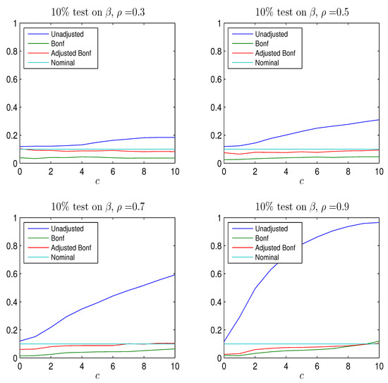
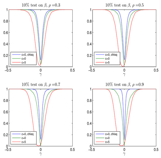
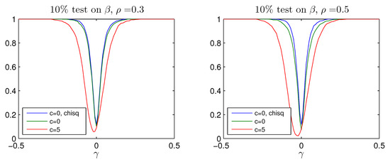
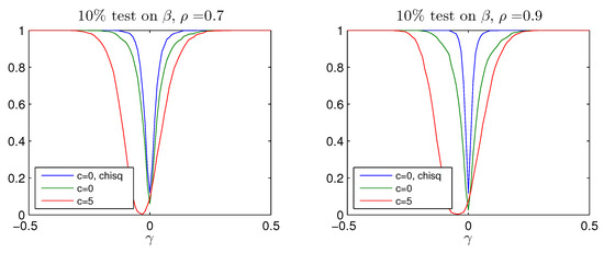
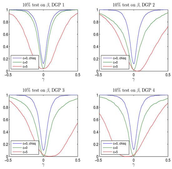
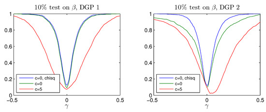
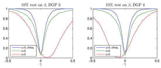
The rejection frequency of the test for calculated using the quantile, the Bonferroni quantile in (20) for and and the adjusted Bonferroni quantile in (21) for is reported as a function of c for four values of in Figure A3. For both corrections the rejection frequency is below the nominal size of ; hence both procedures are able to eliminate the serious size-distortions of the test. While the Bonferroni adjustment leads to rather conservative test with rejection frequency well below the nominal size, the adjusted Bonferroni procedure is closer to the nominal value. The power of the two procedures is shown in Figure A4 and Figure A5 for values of It is seen that the better rejection probabilities in Figure A3 are achieved together with a reasonable power for where the probability of rejecting the hypothesis of is around , see bottom panel of Figure A1. Notice that both tests become slightly biased, that is, the power functions are not flat around the null .
In conclusion, the simulations indicate that the adjusted Bonferroni procedure works better than the simple Bonferroni, the reason being that the former relies on the joint distribution of and .
3.5. A Few Examples of Other DGPs
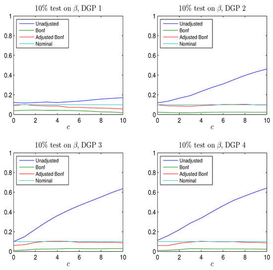
Four other data generating processes are defined in Table 1, to investigate the role of different choices of and for the results on improving the rejection probabilities for test on under the null and alternative. The DGPs all have . The vectors and are chosen to investigate different positions of the near unit root in the DGP.

Table 1.
The matrix for four different DGPs given by which are the basis for the simulations of rejection probabilities for the adjusted test for . The positions of give the different and .
The choice of DGP turns out to be important also for the test, for In fact the probability of rejecting is around for DGP 1 if , for DGP 2 if , whereas for DGP 3 and 4 the value value is 8.
The rejection probabilities in Figure A6 are plotted for to cover the most relevant values.
The results are summarized in Figure A6, Figure A7 and Figure A8. It is seen that the conclusions from the study of the DGP analyzed by Elliott seem to be valid also for other DGPs. For moderate values of using the Bonferroni quantiles gives a rather conservative test while the adjusted Bonferroni procedure is closer to the nominal size and the power curves look reasonable for although the tests are slightly biased, except for DGP 1. For this DGP, such that which means that the asymptotic distribution of is see Theorem 3, despite the near unit root. It is seen from Figure A6, there is only moderate distortion of the rejection probability in this case and in Figure A7 and Figure A8, the power curves are symmetric around so the tests are approximately unbiased.
4. Conclusions
It has been demonstrated that for the DGP analyzed by Elliott (1998), it is possible to apply the methods of McCloskey (2017) to adjust the critical value in such a way that the rejection probabilities of the test for are very close to the nominal values. By simulating the power of the test for it is seen that for the test has a reasonable power. Some other DGPs have been investigated and similar results have been found.
Acknowledgments
The first author gratefully acknowledges partial financial support from MIUR PRIN grant 2010J3LZEN and Stefano Fachin for discussions. The second author is grateful to CREATES - Center for Research in Econometric Analysis of Time Series (DNRF78), funded by the Danish National Research Foundation, and to Peter Boswijk and Adam McCloskey for discussions.
Author Contributions
Both authors contributed equally to the paper.
Conflicts of Interest
The authors declare no conflict of interest.
Appendix A. Proofs
Proof of Lemma 1.
Multiplying by we find
Multiplying by we find
Multiplying by b we find
It follows that from (A2)
and from (A1)
which proves (3) and (4).
Inserting these results in the expression for we find using
Proof of Theorem 2.
The unrestricted maximum likelihood estimator of is and and the results for follow from Lemma 1. If the maximum likelihood estimator can be determined by reduced rank regression, see (Johansen (1996, chp. 6)). ☐
Proof of Theorem 3.
Proof of (7) and (8): The limit results for the product moments are given first, using the normalization matrix and the notation ,
The test for a known value of is given in (6). It is convenient for the derivation of the limit distribution of to normalize on the matrix such that and define This gives the representation
The proof under much weaker conditions can be found in Elliott (1998), and is just sketched here. The estimator for for known and is given by the equation
where The limit distribution of follows from (A5) and (A6) as follows. Because it follows that
and from it is seen that
say. Conditional on the distribution of U is Gaussian with variance and mean The information about satisfies
and inserting U for determines the asymptotic distribution of Conditional on K, this has a noncentral distribution with noncentrality parameter
where which proves (8). The marginal distribution is therefore a noncentral distribution with a stochastic noncentrality parameter, which is independent of the distribution, as shown by Elliott (1998).
Proof of (9): For it is seen that
which proves (9). Note that this expression is zero if and only if or in which case the asymptotic distribution of is
Proof of (10) and (11):
It follows that can be expressed as
where, using (A5) and (A6),
From it follows that
where and This proves (11).
From the normalization we find, replacing by
which proves (10).
Proof of (12): To analyse the limit distribution of , define
and write
The expansion (A7), and the limits (A8) and (A9) are then applied to give the limit results
Thus
Multiplying by and and inverting, it is seen that because and are of full rank,
which proves (12). ☐
Appendix B. Figures
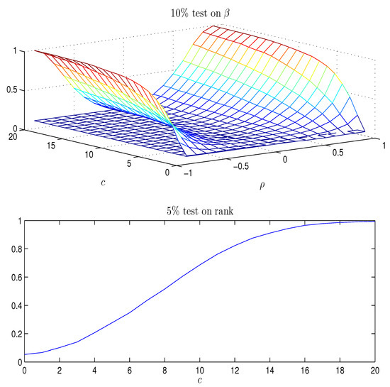
Figure A1.
Top panel: Rejection frequency of the test for using the quantile as a function of c and . Bottom panel: Rejection frequency of the 5% test for using Table 15.1 in Johansen (1996) as a function of c. simulations of observations from the DGP (15) and (16).
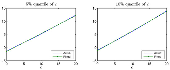
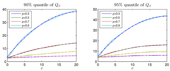
Figure A2.
Quantiles and fitted values in the distributions of and as a function of c for different values of ; simulations of observations from the DGP (15) and (16).
References
- Cavanagh, Christopher L., Graham Elliott, and James H. Stock. 1995. Inference in Models with Nearly Integrated Regressors. Econometric Theory 11: 1131–47. [Google Scholar] [CrossRef]
- Di Iorio, Francesca, Stefano Fachin, and Riccardo Lucchetti. 2016. Can you do the wrong thing and still be right? Hypothesis testing in I(2) and near-I(2) cointegrated VARs. Applied Economics 48: 3665–78. [Google Scholar] [CrossRef]
- Elliott, Graham. 1998. On the robustness of cointegration methods when regressors almost have unit roots. Econometrica 66: 149–58. [Google Scholar] [CrossRef]
- Johansen, Søren. 1996. Likelihood-Based Inference in Cointegrated Vector Autoregressive Models. Oxford: Oxford University Press. [Google Scholar]
- McCloskey, Adam. 2017. Bonferroni-based size-correction for nonstandard testing problems. Journal of Econometrics. in press. Available online: http://www.sciencedirect.com/science/article/pii/S0304407617300556 (accessed on 12 June 2017). [CrossRef]
- Phillips, Peter C. B. 1988. Regression theory for near integrated time series. Econometrica 56: 1021–44. [Google Scholar] [CrossRef]
© 2017 by the authors. Licensee MDPI, Basel, Switzerland. This article is an open access article distributed under the terms and conditions of the Creative Commons Attribution (CC BY) license (http://creativecommons.org/licenses/by/4.0/).