Abstract
The ability to distinguish between sustainable and excessive debt developments is crucial for securing economic stability. By studying US private sector credit loss dynamics, we show that this distinction can be made based on a measure of the incipient aggregate liquidity constraint, the financial obligations ratio. Specifically, as this variable rises, the interaction between credit losses and the business cycle increases, albeit with different intensity depending on whether the problems originate in the household or the business sector. This occurs 1–2 years before each recession in the sample. Our results have implications for macroprudential policy and countercyclical capital-buffers.
Keywords:
debt sustainability; credit losses; financial crises; financial obligations; smooth transition regression; non-linear cointegration JEL Classification:
E32; E44; G01
1. Introduction
The concern that private sector debt accumulations can become excessive, threatening both real and financial stability, has gained considerable momentum during the past decade. To assess the importance of such considerations empirically, one must be able to separate sustainable debt developments from excessive buildups. By studying US aggregate credit loss dynamics over the period 1985–2010, we show that the upper limit for sustainable debt developments is determined by the strength of the incipient aggregate liquidity constraint, as measured by the financial obligations ratio. In particular, we find that both household and business sector financial obligations ratios act as regime switching variables. Once they move beyond critical levels, the interaction between business cycle fluctuations and credit losses starts to intensify. This occurs in either the household or the business sector 1–2 years prior to each economic downturn in our sample. The more severe recessions ensue when both sectors are affected simultaneously. In contrast to existing cross-sectional studies on individual episodes of financial distress, we do not find that leverage, as measured by the debt to income ratio, to be informative in this respect. These patterns suggest that increasing liquidity problems associated with excessive aggregate debt accumulations can undermine both real and financial stability.
The idea that credit cycles can be a source of real fluctuations is by now well established in a large body of theoretical work on financial frictions. For instance, Bernanke et al. (1999) show that feedback between firms’ net worth and their borrowing opportunities can generate credit booms which result in increased investments. Similarly, by focusing on households, Kiyotaki and Moore (1997) demonstrate that increases in house prices raise the value of collateral available to households, increasing their borrowing opportunities and thereby their consumption spending. In both cases, there is a financial accelerator effect which tends to reinforce the business cycle. More recent contributions along these lines include Kiyotaki and Gertler (2010), and references therein.
While the aforementioned literature is mainly concerned with the amplifying effect of credit on ordinary macroeconomic shocks, there is also a risk that aggregate debt can reach excessive and inefficient levels. For example, Lorenzoni (2008) and Miller and Stiglitz (2010) discuss how self-reinforcing processes between net worth and borrowing can lead to asset price bubbles and excessive leverage under the assumptions that agents have limited commitment in financial contracts or dispersed beliefs. Because banks can have incentives to reduce their lending standards during upturns, the problem may be further exacerbated (Ruckes 2004; Dell’Ariccia and Marquez 2006). When aggregate debt reaches unsustainable levels, debt holders become highly vulnerable to any common negative shock which reduces their net worth, as it constrains their refinancing ability. In such situations, they may attempt to sell off assets and reduce spending to meet their debt obligations. Campello et al. (2010), for instance, document such alterations in behavior among financially constrained firms during the recent financial crisis. However, such actions can be contagious as they tend to reinforce the negative effects of the initial shock, triggering off a self-reinforcing downward spiral which can lead to a severe recession or even a systemic financial crisis (e.g., Gai et al. (2008)).
Theoretical predictions of this type have been lent considerable credibility by empirical studies that find a close association between high aggregate debt to income ratios (leverage) and subsequent credit and output losses1. For example, King (1994) documents this type of relationship across countries in connection with the early 1990s recession. More recently, Mian and Sufi (2010) obtain similar results by exploiting US cross-county variation from the recent financial crisis. However, because these studies focus on cross-section variation from individual episodes of financial distress, they tend to overlook the persistent upward trend that has been present in US debt to income ratios for the past 30 years. Because such long-run developments probably impinge on the cross-section in a uniform way, most of the cross-sectional variation will be due to possibly excessive short-run accumulations. If so, this would explain why the past studies find a seemingly close relationship between leverage and losses. The question remains, however: If high aggregate leverage was one of the major factors behind the early 1990s recession, as suggested by King (1994), then how could even higher and increasing debt ratios be sustained during the two following decades?
To make progress, it seems crucial to be able to distinguish between sustainable and excessive debt developments already from the outset. This is recognized by Borio and Lowe (2002) and Borio and Drehmann (2009) who construct early warning indicators of systemic banking crises based on leverage and asset price gaps. While the indicators perform well both in and out of sample, the gaps are, however, constructed using the Hodrick-Prescott filter rather than motivated by economic rationale. Thus, there is a risk of mistaking sustainable debt developments for excessive buildups. For example, if a credit boom lasts for a long time the filtered trend will eventually catch up, producing a gap which is close to zero or even negative. Similar problems can occur if the true underlying trend in debt-to-income suddenly changes. This suggests that the debt to income ratio should be detrended using economic rather than statistical criteria.
The most likely explanation for the upward trend in leverage during the recent decades is the concurrent decline in real interest rates, documented for example in Caballero et al. (2008), among others. Indeed, the optimal (sustainable) allocation of aggregate debt in a dynamic stochastic environment should vary with changes in the terms of credit (see e.g., Stein (2006)). If this is the case, a more appropriate alternative measure for the burden imposed by private sector indebtedness is given by the financial obligations ratio constructed by the Federal Reserve (see Dynan et al. (2003)). By consisting of interest payments and repayments on debt divided by income, the financial obligations ratio captures the incipient aggregate liquidity constraints of borrowers (Hall 2011). Rising financial obligations, for instance, indicate that borrowers have less leeway to smooth their consumption or make new investments, and are also more vulnerable to income and interest rate shocks. This may not be a problem as long as the business cycle is benign and banks’ lending standards are soft. However, when the business cycle turns, the liquidity constraints start to bind for more and more borrowers, forcing them in arrears and ultimately to default, thereby driving up banks’ losses.
To investigate this possibility, we compare the ability of the financial obligations ratio for explaining US banking sector credit losses with that of the debt-to-income ratio. Focusing on credit losses instead of output losses also allows us to assess the differential roles that business and household loans play in generating real and financial weakness (see e.g., Iacoviello (2005))2. We allow the two debt measures to enter credit loss determination both linearly, in line with the literature on financial accelerators, as well as non-linearly, to capture altered behavior and contagion effects during episodes in which aggregate credit constraints become binding. In the latter case, each debt measure is allowed to enter the empirical model as a regime switching variable which smoothly increases the interaction between credit losses and the business cycle once it exceeds an estimated critical threshold.
Applying this approach to quarterly US data from 1985Q1 to 2010Q2, we find evidence of significant nonlinearities in the credit loss data, associated with the episodes of severe financial distress in our sample. This seems consistent with theories that allow for excessive aggregate buildups of credit. However, we do not find any significant temporal relationship, linear or otherwise, between aggregate leverage and credit losses. Replacing leverage by the financial obligations ratio, we find that the latter significantly enters credit loss determination as a regime switching variable of the type described above. Hence, based on this variable we can adequately account for the nonlinear dynamics inherent in aggregate credit losses. In addition, we are able to accurately estimate the parameters of the transition function which determines the weights given to the high and low credit loss regimes as a smooth function of the financial obligations ratio. We refer to the half way point between regimes as the maximum sustainable debt burden (MSDB).
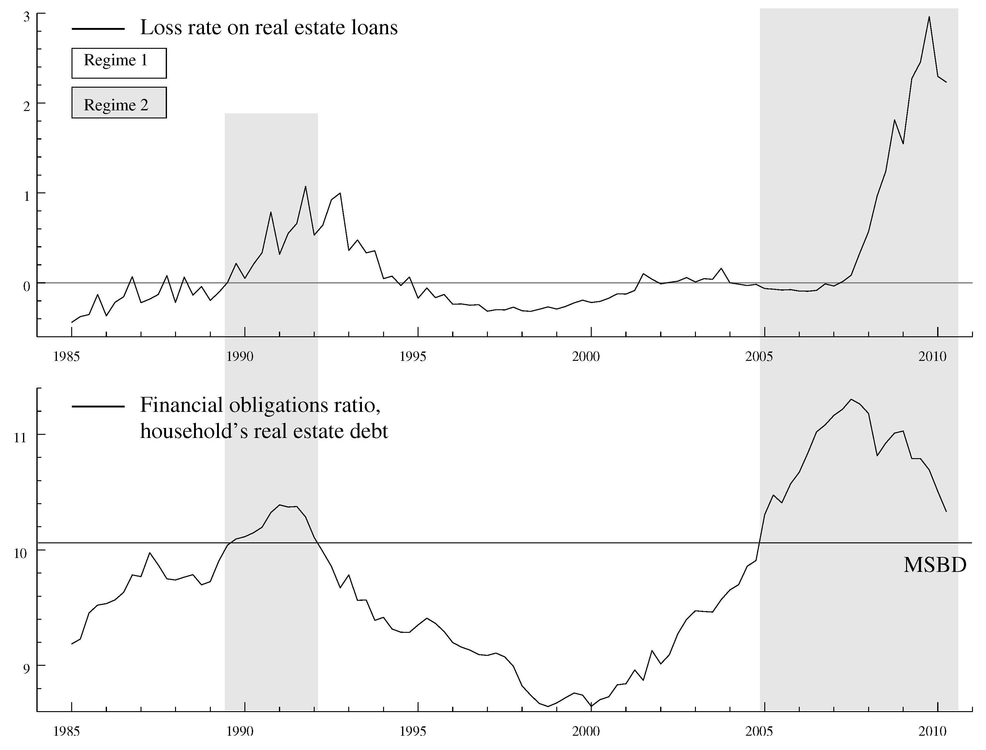
By further distinguishing between total debt and real estate related debt in both the household and business sector, we gain important insights into how these different debt categories contribute to aggregate credit loss dynamics. For the household sector we find that the financial obligations ratio, specifically associated with real estate debt, exceeds an estimated MSDB threshold of 10.1% at two intervals over the sample period. The first interval is 1989Q2–1992Q1, i.e., MSDB is exceeded roughly one year prior to the recession in the early 1990’s and returns to the sustainable region at the bottom of the recession. The second starts in 2005Q1, more than two years before the recent crisis, and continues to the end of the sample in 2010Q2, by which time the financial obligations ratio has not yet returned to the sustainable region. Both of these episodes are associated with massive credit losses and an unusually large number of bank failures, but differ with respect to the severity and length of the ensuing recession. This difference appears to be related to size with which the financial obligations ratio exceeded the MSDB estimate on each occasion.
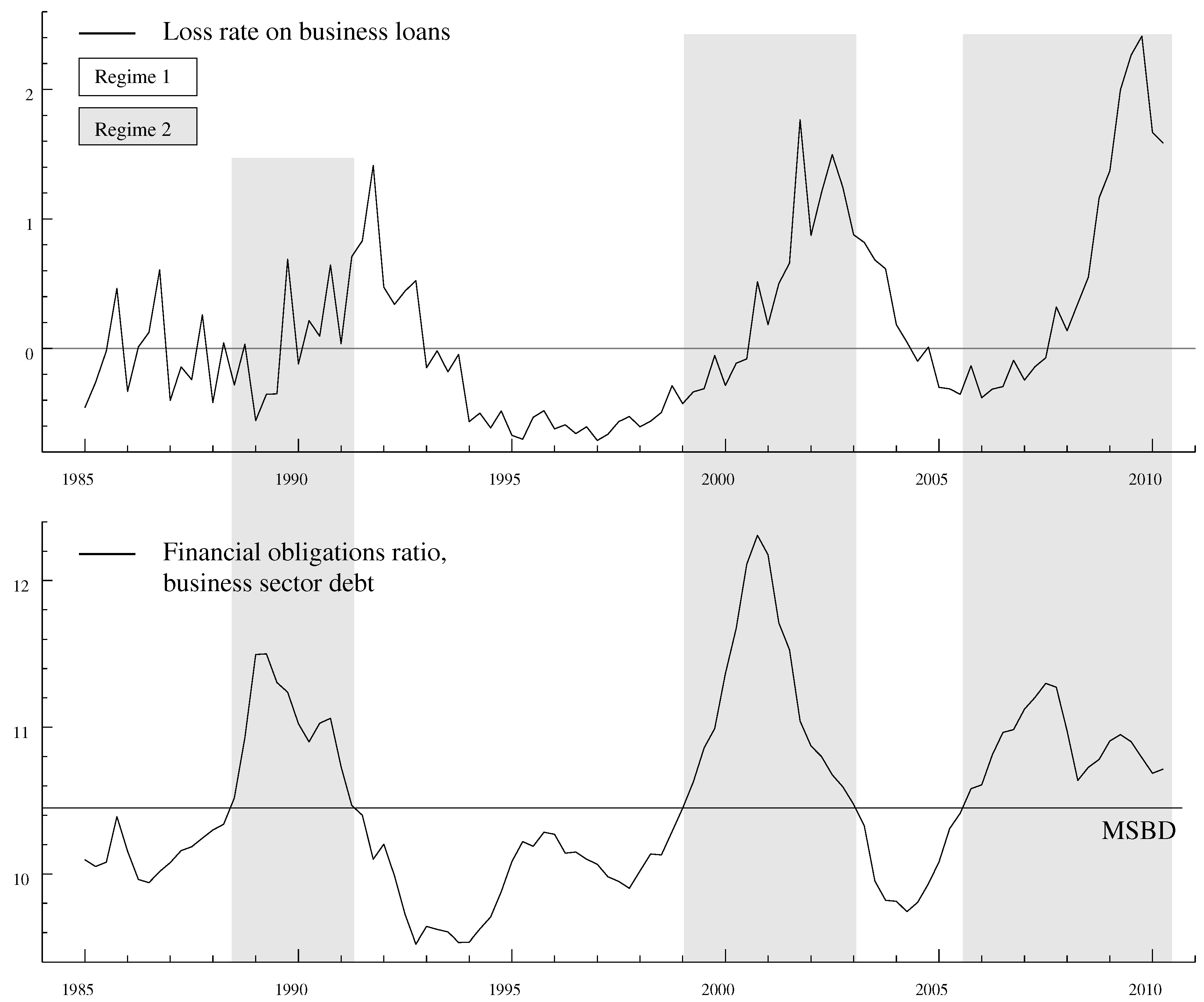
For the business sector, we similarly find that major credit losses ensue when the associated financial obligations ratio crosses its MSDB estimate of 10.4% into the unsustainable region. This happens 1–2 years prior to each of the three US recessions in the sample but, as exemplified by the recession in the early 2000s, does not necessarily lead to large-scale bank failures. While the credit losses associated with excessive business loans seem less detrimental to financial stability than those associated with households’ real estate loans, they may, nevertheless, exert a significant effect on the business cycle.
The observation that the financial obligations ratio in excess of its MSDB level precede economic downturns could be useful in designing capital standards for banks (Drehmann et al. 2010; Repullo et al. 2010) and for implementing more general macro prudential policies (e.g., Borio (2009)). For instance, our analysis suggests that credit risk assessment based on financial obligations ratios could lead to more countercyclical capital standards. Similarly, the financial obligations ratios, in particular those related to real estate debt, may be useful for macro prudential policy as early warning indicators of such long-term debt accumulations which may eventually threaten financial stability3. Our results also suggest a channel through which monetary policy may affect financial stability under certain conditions. For instance, an interest rate increase, intended to curb inflationary pressure, can impinge on financial stability in periods when aggregate debt is close to or above the sustainable level. This is because an interest rate increase directly raises the financial obligations of borrowers, which in turn can make credit losses both more likely and more severe.
2. Data
This section introduces quarterly US time-series data of the key variables, spanning the sample 1985Q1–2010Q2. We first introduce credit loss rates and indicators of the business cycle, and discuss their temporal association graphically. Then, in Section 2.2, we present two different measures of aggregate debt and relate their dynamics to that of the credit loss rates. Detailed descriptions of the variables and their sources are provided in Appendix A.
2.1. Credit Losses and Business Cycle Indicators
As a measure of credit losses we use the net charge-off rate on loans held by all insured commercial US banks. The banks are required to charge off an estimate of the current amount of loans and leases that are not likely to be collected, or are more than 120 days delinquent, from their loan loss allowance4. The net change-off rate is the current period change-offs minus recoveries. Hence, it constitutes the most accurate and timely estimate of credit losses that are available for US banks.
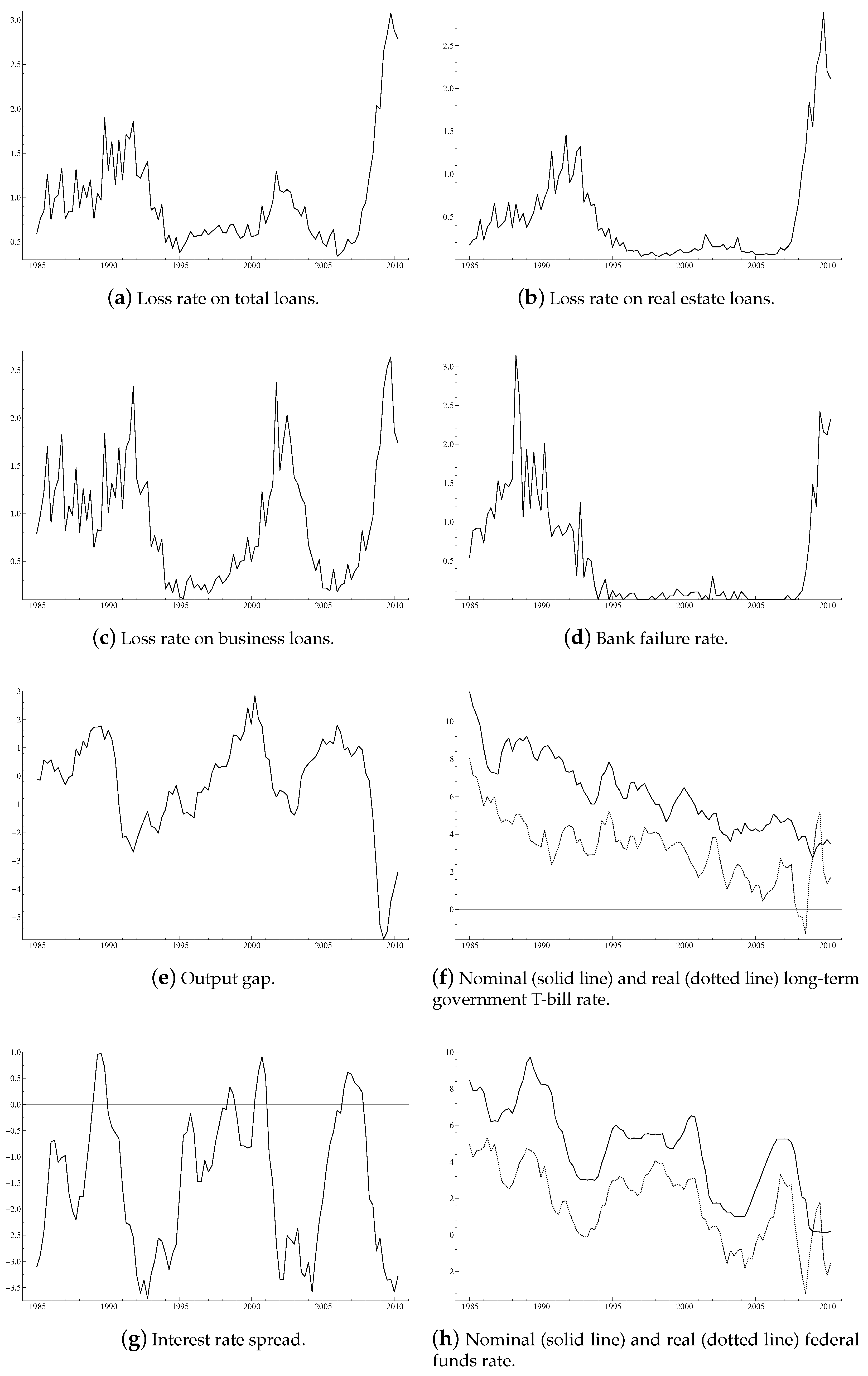
We distinguish between losses on total loans (TL), real estate loans (RL), and business loans (BL), denoted , , and , respectively. The loss rate on total loans, depicted in panel (a) of Figure 1, shows peaks at the low point of each of the three US recessions in the sample (as indicated by a standard output gap measure, , depicted in panel e of the figure), with the most recent one being almost twice as severe as the previous ones. This pattern, however, is not preserved over different loan categories. For example, the loss rate on real estate loans (panel b) peaks only twice over the sample, first during the recession in the early 1990s and next during the recent financial crisis. As can be seen from panel (d) of the figure, both of these occasions are associated with large-scale bank failures. In contrast, the loss rate on business loans (panel c) displays peaks of roughly equal magnitude at each of the three recessions. In this sense, it more closely resembles the term-spread, , depicted in panel (g), where is the federal funds rate and is the yield of 10-year treasury securities. We also note that losses on business loans seem less strongly connected to bank failures, as exemplified by the early 2000s recession.
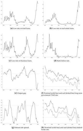
Figure 1.
Credit loss rates and various indicators of financial, monetary, and real conditions in the United Sates. The real (ex-post) interest rates are constructed using the 4-quarter moving average inflation rate to facilitate the exposition.
This ocular evidence suggests that there may be significant interactions between credit losses across different loan categories and the business cycle, potentially reinforcing each other. For instance, deep recessions and financial instability appear to be more closely associated with losses on real estate loans than losses on business loans, whereas the latter seems more related to ordinary business cycle fluctuations. The question is whether a suitable measure of the aggregate debt burden, either the conventional leverage or the financial obligations ratio that we propose in this paper, can predict when such interactions become pivotal5.
2.2. Leverage vs. Financial Obligations
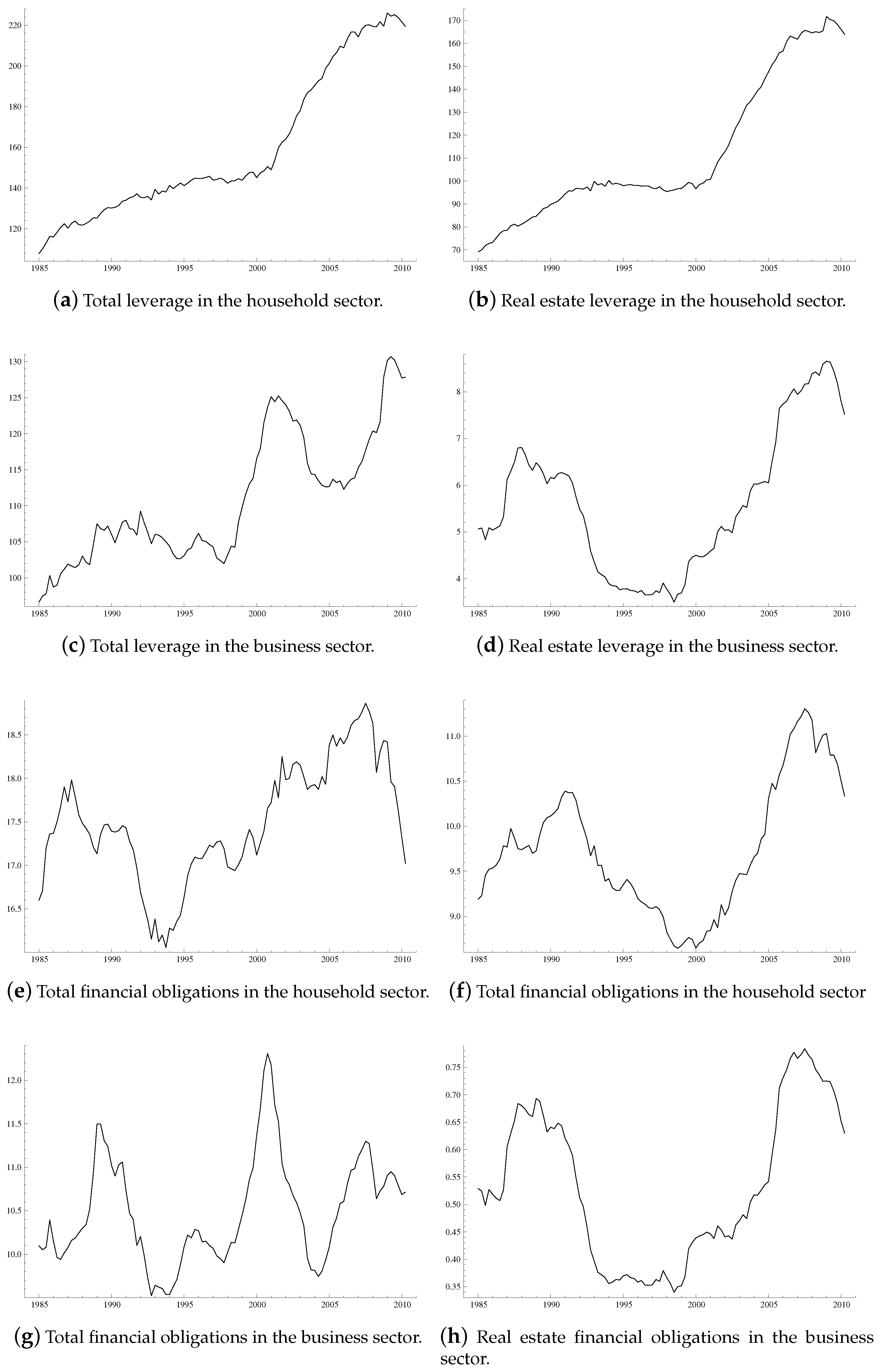
Panels (a)–(d) in Figure 2 depict the household (H) and business (B) sector debt-to-income ratios, distinguishing between total and real estate loans (RL), respectively. We use these ratios as a measure of leverage and denote them by , where and . By comparing panels (a) and (b), as well as panels (c) and (d), it can be seen that real estate loans comprise more than two thirds of total loans in the household sector, but less than 10% of total loans in the business sector. Moreover, business sector leverage appears to be more volatile than household sector leverage. This points to potentially important disparities between the processes which generate excessive debt in the two sectors.

Figure 2.
Indicators of leverage and financial obligations in the household and business sectors.
One potential problem with using the leverage variables for determining debt sustainability is their clear upward trends over the sample. This either implies that debt in the two sectors did not reach excessive levels until possibly just before the recent crisis or, alternatively, that the associated critical threshold must have been time-varying. The evidence in King (1994), for example, would argue against the former case, whereas estimation is problematic in the latter.
The likely reasons for the growth displayed by the debt-to-income ratios are changes in the terms of credit, as discussed in the introduction. For instance, both the federal funds rate and the long-term interest rate have been declining over the entire sample, as is evident from panels (f) and (h) in Figure 1.
A measure that explicitly accounts for changes in the terms of credit is the financial obligations ratio, reported by the Federal Reserve. It is broadly defined as the ratio of financial obligations, consiting mostly of interest payments and amortizations, to income6. As the Federal Reserve only reports this measure for the household sector, we construct a corresponding measure for the business sector by using the federal funds rates as the relevant interest rate, a fixed maturity of 3 years7, and a linear amortization schedule. Panels (e)–(h) in Figure 2 depict the financial obligations ratios, denoted by , where i corresponds to the two sectors and j to the two loan categories. These ratios show less persistent growth and a stronger tendency to revert back to some benchmark value, compared to the leverage variables. Moreover, given that a large fraction of debt outstanding has longer maturity than one quarter, the per-period financial obligations ratios are considerably lower than the corresponding debt to income ratio as can clearly be seen from the figure.
The differences in the dynamic behavior between the leverage variables and the financial obligations ratios indicate that much of the upward trend in the former is due to changes in the terms of credit. Hence, the financial obligations ratio is more likely to be informative about the limits to private sector indebtedness than leverage.
3. Methodology
In this section, we present our empirical strategy for determining the role of aggregate debt variables in credit loss determination and discuss statistical models which can be used for its implementation. We first document that our credit loss variables display considerable variability at frequencies close to zero. This suggest that standard cyclical variables, such as output gaps or credit spreads, may not be able to fully account for the variation in them. We then consider two alternative sources for the persistence, both related to the aggregate debt variables.
The first possibility is that the persistence of the credit loss rates is directly (linearly) inherited from the debt variables. This would be in line with existing empirical work on financial accelerators (e.g., Gertler and Lown 1999; Gilchrist et al. 2009). Because the economic models which underlie such accelerator effects typically exclude credit rationing (see e.g., Bernanke et al. (1999)), they seem more relevant as descriptions of credit market and business cycle interactions during normal (stable) times. To allow for this possibility we approximate the persistence in the credit loss rates and the debt variables by unit-roots and test for cointegration between them.
If the persistence cannot be accounted for linearly, a second possibility is that it stems from threshold dynamics related to excessive debt. For example, Leybourne et al. (1998) and Nelson et al. 2001 find that such non-linear dynamics can give rise to the appearance of stochastic trending. To study this possibility, we use the debt measures as transition variables in nonlinear regime-switching models for the credit loss rates. The idea is to capture increases in the interaction between credit losses and the business cycle which may arise if aggregate debt is allowed to reach excessive levels (see e.g., Miller and Stiglitz (2010)). The reason is that borrowers who are at the limits of their credit constraints may not be able to smooth their consumption or make optimal investments as they have to honor their debt obligations in the wake of a negative shock. Campello et al. (2010), for example, document significant changes in the investment and employment decisions of credit constrained firms during the recent financial crisis. If the proportion of constrained borrowers is large, this type of behavior can easily reinforce the negative effects of the initial shock, thereby creating increased feedback between loan defaults and the business cycle. An additional benefit of this modeling strategy is that it allows us to estimate a critical threshold for each debt variable above which it becomes excessive, provided that nonlinear transition-dynamics are present8.
3.1. Statistical Models
A convenient way of testing for linear long-run co-movement between the credit loss rates and the debt variables is to model them jointly in a cointegrated VAR model
where for , is successively one of the debt measures presented in Section 2.2, i.e., or for and , is a vector consisting of a constant and seasonal dummies (and possibly other dummies defined in the text), , and k is the lag-length. This setting implies that we only consider each debt variable separately rather than jointly. Note that we also include the federal funds rate as a separate variable in the system. This is to allow for possibility that the decline in interest rates over the past decades have reduced credit risks associated with the existing stock of loans in banks’ loan portfolios (see e.g. Altunbas et al. (2010)).
Cointegration in (1) can be tested by the likelihood ratio (LR) test for the rank of (Johansen (1996)). If the rank, r, is equal to the number of variables in the system, p, then is stationary, i.e., . If , then , where and are two matrices of full column rank and describes the cointegration relationships. In this case and cointegrated with r cointegration vectors, , and common stochastic trends, assuming that the “no trends” condition is met, where ⊥ denotes orthogonal complements. For example, any variable in that is stationary a priori, such as the term spread and the output gap, is expected to increase r by one and add a unit-vector to . If , then and the process is not cointegrated. A testing sequence that ensures correct power and size starts from the null hypothesis of rank zero and then successively increases the rank by one until the first non-rejection. When , it is possible to test the hypothesis that a variable, say, is weakly exogenous with respect to the long-run parameters of the model. The test of this hypothesis is asymptotically , and amounts to imposing zero-restrictions on a row of corresponding to .
If the persistence in the credit loss rates cannot be explained linearly, there is still a possibility that it stems from important nonlinearities. To allow for this possibility, we specify a smooth transition regression (STR) model for the credit loss rates. As we do not expect to find strong nonlinearities in the other variables9, we focus on a single-equation model to keep the analysis tractable, rather than attempt to estimate a full-fledged multivariate STR model (see van Dijk et al. (2002)). In particular, the model takes the form
where, is a vector of potentially difference stationary explanatory variables, is a vector of deterministic terms define above, and is assumed to be a mean zero stationary disturbance term10. We note that the stationarity assumption on the disturbance term implies that and are either linearly or non-linearly cointegrated. Thus, verifying this assumption ensures model consistency, as well as safeguards against spurious results, for example due to growth correlations over time.
Our primary interest lies in the transition function
which determines the relative weights between regimes 1 and 2, and has the properties and . We use as the primary transition variable, i.e., we successively try one of the leverage or financial obligations ratios as arguments in 11. Hence, for positive and , say, (2) captures gradual changes in the effect (given by ) of the cyclical variables in on credit losses, as the debt variable increases. The halfway point between regimes, which we will loosely refer to as the maximum sustainable debt burden (MSDB), is determined by the and the speed of the transition is determined by .
We apply a linearity test by Choi and Saikkonen (2004) to identify the statistically significant transition variables. The test is based on a Taylor series approximation of (2), which under the null hypothesis of linearity will not contain any significant second (or higher) order polynomial terms. However, under the STR alternative, all significant higher order terms will involve the transition variable. Hence, statistically valid transition variables can be detected by applying the test successively to each variable from the set of potential transition variables. Such information may be helpful in distinguishing between competing explanations for the recent crisis, such as lax monetary policy or excessive debt.
4. Results
This section reports the main empirical findings. Section 4.1 first investigates whether the observed persistence in the credit loss rates is due to exogenous factors or related to (transitory) regime shifts, or both. Next, Section 4.2 compares the ability of leverage and the financial obligations ratio for explaining shifts in credit loss dynamics. Section 4.3 reports the estimates associated with regime shift dynamics, and shows that they are informative about debt sustainability.
4.1. Linearity vs. Regime Shifts
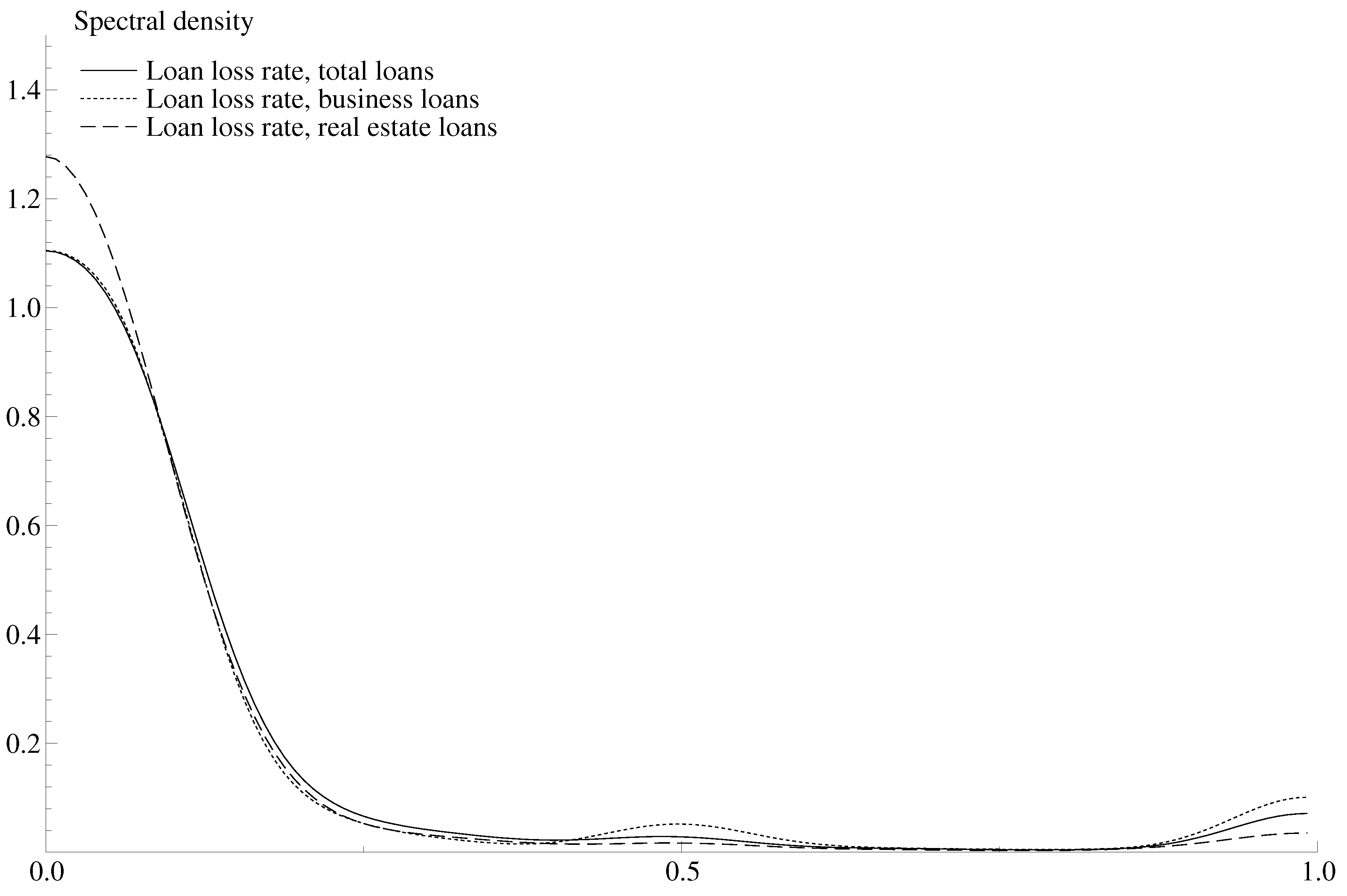
We find that all credit loss rates show significant variation at frequencies close to zero, indicating the presence of cycles of longer duration than the available sample. This can be clearly seen from the spectral densities reported in Figure 3. Moreover, the unit-root hypothesis cannot be rejected for any of the loss rates using standard Augmented Dickey-Fuller (ADF) tests. We also find that our leverage variables, financial obligations ratios, and the federal funds rate (see Figure 1 and Figure 2) all display similar stochastic trending12. Hence, each of the latter variables may conceivably be a source of persistence in the credit loss rates.
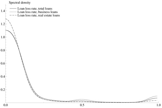
Figure 3.
Spectral densities of the credit loss rates.
While unit-roots are a convenient way of capturing the persistence in the credit loss rates, giving such roots a structural interpretation in this context does not seem reasonable. Instead, the persistence is more likely to reflect breaks or other types of nonlinearities, possibly associated with the recent crisis and its aftermath. For this reason, we adopt a cautious approach, initially restricting our attention to the pre-crisis sample 1985Q1–2006Q4, where regime shift dynamics are less likely to have played a dominant role in credit loss determination. We model credit loss rates jointly with the other variables to see if we can identify the source of the persistence in them, i.e., we estimate (1) with for and successively indicating one of the debt variables in Section 2.2. We are especially interested to see if the persistent debt variables are relevant in this regard.
Applying the LR test for cointegration rank, as well as tests for unit-vectors in , we find that: (i) unit-roots in the credit loss rates cannot be rejected in the pre-crisis sample; (ii) none of the other persistent debt variables are linearly cointegrated with the loss rates; and (iii) that the output gap and the term spread are stationary (i.e., they have corresponding unit vectors in )13. The only variable that is linearly cointegrated with the loss rates is the nominal federal funds rate, suggesting that the declining interest rates during the past decades have reduced credit risk, consistent with Altunbas et al. (2010).
We next ask if the pre-crisis sample cointegration results continue to hold once the recent crisis period is included. For simplicity, we do this within a smaller model with , , a restricted constant, three centered seasonal dummies, and transitory impulse dummies (reported in Appendix A), but the results remain the same if we also include the stationary variables and the debt variables. Table 1 reports the results of the LR test for the rank of and tests of weak exogeneity (conditional on ). The upper part of the table confirms the cointegration results for the pre-crisis sample. As can be seen, is always rejected, whereas cannot be rejected in this sample. Moreover, we cannot reject the hypothesis that the federal funds rate is weakly exogenous. The lower part of the table shows that the cointegration results break-down in the full sample from 1985Q1 to 2010Q2. This is likely caused by a transitory but influential change in the process that govern short-run credit losses associated with the crisis.

Table 1.
Linear cointegration results. Notes: The rows labeled “” and “” report the p-values of the LR tests for the rank of . The following two rows report the p-values from testing weak exogeneity for both of the variables in . Boldface values indicate significance at the 5% level.
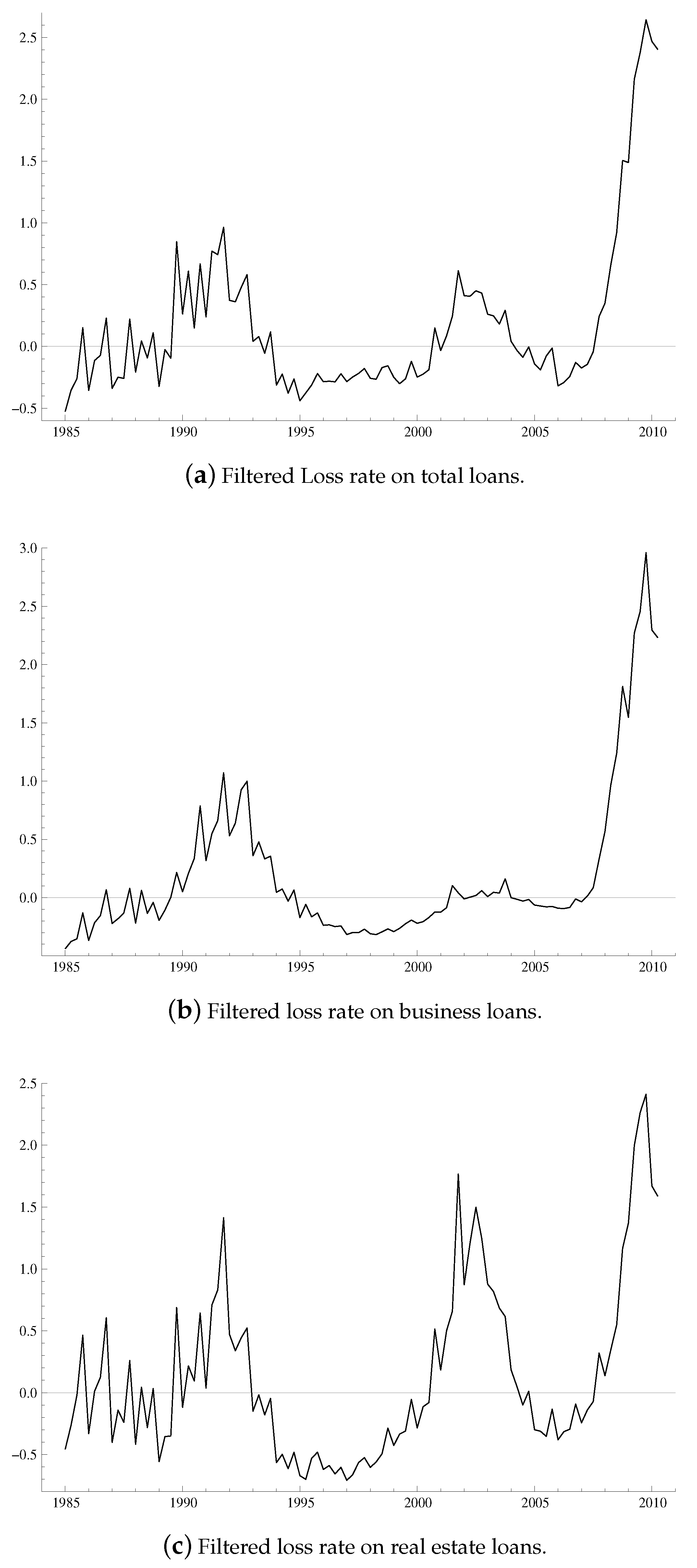
The presence of a small downward trend associated with the long-term decline in the federal funds rate is a nuisance, as there is a risk that it can be mixed-up with the type of nonlinearity that are the main focus of the study. For this reason, we estimate it by Hodrick-Prescott filtering the federal funds rate and remove it from the credit loss rates based on the pre-crisis cointegration estimates14. The adjusted loss rates are depicted in Figure 4. Comparing these loss rates with the unadjusted ones in Figure 1, reveals that the effect of the detrending is relatively small. The main change is a relative reduction in the loss rates at the beginning of the sample compared to the rates at the end.

Figure 4.
Credit loss rates with stochastic trend component removed.
Having controlled for linear stochastic trends in the loss rates, we proceed to test the null hypothesis of linearity against the STR model alternative in (2) using a test by Choi and Saikkonen (2004). Initial modeling suggested that none of the debt variables (which successively enter through ) yielded significant coefficients in or , i.e., the two regimes. Hence, we excluded them from altogether. Similarly, the output gap, , was never significant in the model for the loss rate on business loans, , and was therefore excluded from this model. This has very little effect on the estimated regime switching dynamics, but improves the precision of the and estimates. We consistently apply these restrictions in the subsequent analysis, using in the models for losses on total loans and real estate loans and in the model for losses on business loans.
Given the indicated choices of , Table 2 reports the results of the linearity tests corresponding to each of the individual debt variables. For the pre-crisis period, the results in the upper part of the table show that the null hypothesis of linearity cannot be rejected in any of the models15. However, turning to the lower part of Table 2, we see that the null hypothesis of linearity is rejected for several potential transition variables in the full sample. For instance, in the model for the loss rate on real estate loans, , there seems to be significant nonlinearities associated with household and business sector real estate debt-to-income, as well as the household sector’s real estate financial obligations ratio. In the model for the loss rate on business loans, on the other hand, all debt-to-income ratios and the financial obligations ratio in the business sector, are significant. The results of the model for the loss rate on total loans, are, by and large, a combination of the results from the models of and . Hence, while regime shifts do not play a very dominant role in the pre-crisis period, they seem crucial for describing credit loss dynamics in the full sample, and in particular during the recent financial crisis.

Table 2.
Tests of linearity against a STR alternative. Boldface values indicate rejection of the null hypothesis at the 5% significance level.
4.2. Leverage vs. Financial Obligations
Next we estimate (2) for each the three credit loss rates, , with as in the previous section, and in successively equal to one of the transition variable candidates that has a significant entry in Table 2. Before we turn to the estimates, it is worthwhile to ask if the resulting regressions can account for the persistence in the credit loss rates associated with the crisis period. To this end, we apply both ADF tests and and (KPSS) stationarity tests to the residual. While these tests are strictly not valid for the residuals from (2), which are mixture processes, this technicality may not be so important in practice16. Nevertheless, these results should be viewed with some caution.
When the leverage variables, , are used we find that the stationarity of the residual cannot be secured in most cases. This can be seen from Table 3 which reports (ADF) unit-root and (KPSS) stationarity tests for the residual. In only two cases, in the equation for and in the equation for , do the tests conclusively yield stationary residuals. In both of these cases, however, the estimated parameters of are such that regime 2 never occurs within the sample. In one case ( in the equation for ), the tests yield inconclusive results. These results suggest that non-linear cointegration is generally rejected when the leverage variables are used, implying they cannot adequately account for the large and persistent fluctuations in the credit loss rates associated with the regime-shift dynamics.

Table 3.
Tests for non-linear cointegration. The null hypothesis of the Augmented Dickey-Fuller (ADF) test is that the residual from (2), with explained and transition variable as indicated in the columns, is a unit-root process. A constant and seasonal dummies were included, and lag-length was chosen based in the AIC information criterion. The 10%, 5%, and 1% critical values for this test are −2.58, −2.89, and −3.50, respectively. The null hypothesis of the Kwiatkowski–Phillips–Schmidt–Shin (KPSS) test is that the aforementioned residual is stationary. The bandwidth was set to 2 in each case. The 10%, 5%, and 1% critical values for this test are 0.35, 0.46, and 0.74, respectively. Rejections of the null hypothesis at the 10%, 5% and 1% significance levels are indicated by ⋆, , and , respectively. † Estimated values for and imply that regime 2 occurs outside the rage of .
In contrast, when the financial obligations ratios are used, both the ADF and the KPSS tests conclusively support the stationarity of the residuals as can be seen from Table 3. Moreover, in all of these cases the estimated parameters of yield regime transitions inside the range of the relevant financial obligations ratio. In the model for losses on total loans, both the financial obligations ratios associated with real estate debt in the household and business sectors, and , have significant entries in Table 2. We choose the former financial obligations ratio as it produces a somewhat better fit and higher likelihood than the latter. Based on these results, the leverage variables do not seem to signal an impending crisis with sufficient precision, whereas the Financial obligations ratios seem more relevant in this respect.
4.3. Explaining Credit Losses
Table 4 reports the key parameter estimates of the STR models. As can be seen from the table, both the estimated coefficients measuring the speed of transition between regimes, , and the estimated thresholds, , are positive, indicating that regime 2 dominates for values above . Furthermore, the estimates of indicate that speeds of transitions between regimes are rather fast in all cases. The two regimes are characterized by the parameters and , describing the effect of of the term spread, and the output gap, , on credit losses, , in each regime (except in the equation for where only enter the regimes). The parameters in the first regime are generally negative but not significant, whereas in the second regime both parameters become negative and significant. It is notable that the effect on credit losses from a change in the output gap or the interest rate spread is much larger in the second regime. Therefore, the financial system becomes much more exposed to real economic fluctuations when the financial obligations ratios are above the estimated threshold values. Thus, the second regime describes unstable periods where even small negative shocks can lead to massive credit losses. In this sense, the threshold values, , can be viewed as estimates of the maximum sustainable debt burden (MSDB) with respect to a given credit category. Our estimates suggest that both total debt and real estate debt become unsustainable (i.e., susceptible to high loss rates) when the financial obligation ratio associated with households real estate loans exceed 10.19% and 10.08%, respectively. Similarly, business debt becomes unsustainable when the financial obligations ratio associated with total business loans exceeds 10.44%.

Table 4.
Estimated transition parameters and regime coefficients from STR models of the adjusted credit loss rates. Boldface values indicate significance at the 5% level (standard errors in parenthesis).
The results in Table 4 are robust to more general specifications of (2). For example, adding auto-regressive lags to the equation yields a well-specified model with approximately constant parameters that displays both quantitatively and qualitatively similar results. Moreover, the model also compares favorably to a simple Markov-Switching specification of (2). This suggests that conditioning the transition dynamics on the financial obligations ratio is indeed beneficial for describing credit loss dynamics. The details of these robustness checks are reported in Appendix B.
The relationship between the financial obligations ratio and the credit losses can also be presented graphically. The upper panel of Figure 5 depicts the loss rate on real estate loans, and the lower panel depicts the financial obligations ratio related to household real estate debt along with a line demarking the corresponding MSDB estimate. The periods during which the second regime dominates are demarked by grey bars in the figure. As can be seen, there are only two unstable periods in the sample. The first begins in 1989Q2, roughly one year in advance of the recession in the early 1990s, and ends at its bottom. The second begins in 2005Q1, over two years in advance of the recent crisis, and has not yet ended by the last observation in our sample (2010Q2). Hence, in retrospect this MSDB estimate would have signaled a significant increase in credit risk a full two years before the onset of the crisis. In addition, the magnitude and duration by which the financial obligations ratio exceed the MSDB line may explain both the severity and length of the ensuing downturns. We leave this interesting aspect for future work.
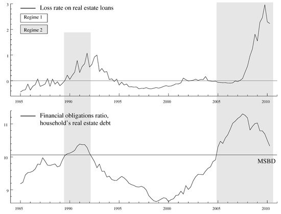
Figure 5.
Transitions in the loss rate on real estate loans. The upper panel depicts the loss rate on real estate loans, whereas the lower panel depicts the financial obligations ratio associated with household’s real estate debt and the corresponding MSDB estimate. Episodes when regime 2 dominate are demarked by grey bars.
Similarly, Figure 6 depicts the loss rate on business loans and the corresponding financial obligations ratio. As can be seen form the figure, there are three unstable periods in our sample, each beginning between 1–2 years prior to one of the three known US recessions in the sample, and ending roughly at their low points. Prior to the 1990s recession, the MSDB of business loans is exceeded in 1988Q2, a full year earlier than the MSDB of households real estate loans. However, prior to the recent crisis the relative timing is reversed, i.e., the household sector MSDB was exceeded first. Finally, we note that it is possible to construct the business sector financial obligations ratio for earlier dates than those in our estimation sample. Hence, as a tentative test of the out-of-sample performance of the business sector MSDB, we checked whether it predicts the deep recession in the early 1980’s17. We find that the financial obligations ratio crosses the MSDB line from below in 1980Q4, three quarters before the onset of the early 80’s recession, and returns to the sustainable region at bottom of the recession. Since this pattern is in accordance with the within-sample results, it gives some additional support to our estimates.
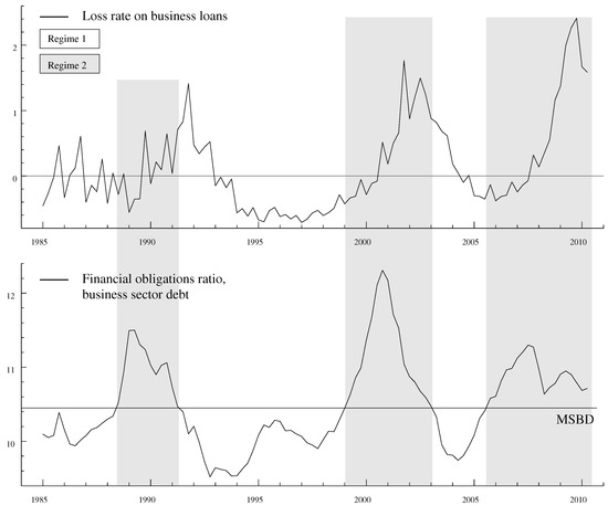
Figure 6.
Transitions in the loss rate on business loans. The upper panel depicts the loss rate on business loans, whereas the lower panel depicts the financial obligations ratio associated with total business sector debt and the corresponding MSDB estimate. Episodes when regime 2 dominate are demarked by grey bars.
5. Conclusions
When do aggregate debt accumulations become excessive, compromising both macroeconomic and financial stability? By studying US credit loss dynamics over the period 1985–2010, we show that it is the strength of the aggregate liquidity constraint, as measured by the financial obligations ratio, which determines the upper limit for sustainable debt developments. In contrast to previous studies which use cross-sectional data, we do not find the debt-to-income ratio, or leverage, to be particularly relevant in this respect. The reason for this finding seems to be that a large part of the growth trend in leverage during the past decades was in fact sustainable and due to a concurrent decline in the real interest rate. Because this trend is likely to have a uniform effect on the cross-sections, most of the cross-sectional variation in leverage will be due to excessive buildups which, thereby, generate seemingly strong association with subsequent credit losses.
We find that the private sector financial obligations ratio displays a cyclical pattern, reaching unsustainable levels 1–2 years prior to each of the three US recessions in our sample. This pattern is, however, not identical among households and businesses. For instance, the household sector cycle seems to be approximately twice as long as the corresponding business sector cycle. Thus, the household sector financial obligations ratio only reached unsustainable levels prior to the deep recessions in the early 1990s and late 2000s, whereas the Business sector financial obligations ratio reached unsustainable levels prior to each of the three recessions. These results suggest that the distinction between excessive financial obligations in the household and business sectors may be important for understanding why some recessions become deep and prolonged while others do not. However, They also indicate that the financial obligations ratio may be useful as an early warnings indicator.
While our empirical approach seems promising in the sense of successfully spotting buildups of excessive aggregate debt, several interesting avenues for future research remain to be explored. For instance, because different types of households are likely to differ with respect the tightness of their financial constraints (Hall (2011)), it might be worthwhile to decompose the financial obligations ratio according to such characteristics as age and income. This may significantly improve our ability to detect excessive debt accumulations, especially when population cohorts change along these dimensions. It is also conceivable that our framework can be extended to an analysis of public sector debt, which could potentially be very valuable in light of the ongoing US and European sovereign debt crisis. As a final remark, we note that the recurrent nature of excessive debt accumulations suggests that the underlying credit market behavior is systematic, which seems inconsistent with the basic assumptions of most theoretical models. Asset price models that incorporate imperfect knowledge and heterogeneous expectations (e.g., Frydman and Goldberg (2009) and Burnside et al. (2016)) are able to generate pervasive boom and busts as a consequence of the market’s allocation of capital and, hence, seem more promising in this respect.
Acknowledgments
We thank Michael Goldberg and Katarina Juselius for giving us extensive feedback on an earlier version of this paper. We have also benefited from numerous valuable comments and suggestions provided by Sigbjørn Attle Berg, Claudio Borio, Diana Bonfim, Stephen Cecchetti, Andrew Filardo, Staffan Ringbom, Jerome Stein, Paul Wachtel, and participants at presentations given at the Bank for International Settlements, 17th Dubrovnik Economic Conference, Bank of Finland, Norges Bank, Van Leer Jerusalem Institute, the 14th DNB Annual Research Conference, and 21st EC-squared conference. Remaining errors and omissions are our own.
Author Contributions
Mikael Juselius and Moshe Kim developed the analysis and drafted the article. Mikael Juselius collected the data, implemented the analysis in CATS in RATS, PcGive and GAUSS, and interpreted the results. Both authors contributed to the critical revision of the article.
Conflicts of Interest
The authors declare no conflict of interest.
Appendix A
Detailed definitions of the variables used in the analysis are provided in Table A1.

Table A1.
Variable definitions and sources.
Table A1.
Variable definitions and sources.
| Data and Definitions | |
|---|---|
| Variable: | Definition: |
| Net charge-off rate on loans, all insured US commercial banks. h = TL (total loans), RL (real estate loans), and BL (business loans). Source: FRS (Bank Assets & Liabilities) | |
| Debt-to-income ratio (in %). (households’), B (Nonfarm nonfinancial corporate business). (total loans), (real estate loans). Household income: total wages and salaries. Business income: Value added in non farm business. Sources: FRS (Flow of Funds Accounts) and BEA (National Economic Accounts). | |
| Financial obligations ratio. i and j are as above. For the series are taken from the FRS (Household Finance). For the definition is . | |
| Effective federal fund rate (3-month average). Source: FRS (Interest Rates) | |
| Yield on 10-year Treasury securities. Source: FRS (Interest Rates) | |
| , where is log real output and is the OECD production function | |
| based level of potential output. Source: OECD. | |
Sources: Federal Reserve System (FRS), Bureau of Economic Analysis (BEA), Bureau of Labor Statistics (BLS), OECD databases (OECD), Federal Housing Finance Agency (FHFA).
The underlying data are publicly available at the listed sources. To check robustness, we considered several alternative measures. For instance, we used the household debt service ratio (FRS) instead of , deviations between real and Hodric-Prescott filtered GDP and the unemployment gap (congressional budget office definition) instead of , and the difference between corporate BAA and AAA bonds instead of . This did not produce significant changes to the results.
A few transitory impulse dummies were used in connection with the VAR estimates in Section 4.1. These dummies (labeled ) take the value 1 at date and –1 at the consecutive date, where and Q refer to the year and quarter digits, respectively. The model for includes , the model for includes , and , and the model for includes and .
Appendix B
In this section we test robustness of the results reported in the main text with respect to alternative specifications. We begin by comparing the results in Table 4 with those obtained from a dynamic specification of (2). We also report the results from break-point Chow tests for these models. Finally, to assess the value added of the financial obligations ratios for explaining regime-switching in credit loss rates, we compare the weights to Regime 2 from models in Table 4 with the ones obtained from a simple Markov-Switching (MS) dynamic regression specification of (2).
The results in Section 4.2 indicate that the STR models for the credit loss rates in conjunction with the financial obligations ratios can produce stationary residuals. These residuals are, however, severely auto-correlated and show other signs of misspecification as well. As this can affect both the precision and consistency of the estimates reported in Table 4, we re-estimate the STR models using a dynamic specification of the form
where for , and and are as in Section 4.3. Table A2 reports the estimates. As can be seen from the table, the estimated parameters of the transition function, and , are fairly close to the ones reported in Table 4. The biggest difference with respect to these parameters occurs in the model for losses on real estate loans, where increases from 10.08 to 10.92. While this increase is substantial, the speed of adjustment is now reduced from 3.61 to 2.50. This has the effect of widening the transition region, producing very similar regimes as before. At the same time, however, it becomes less appropriate to interpret as a maximum sustainable debt burden.
The effect of the explanatory variables, as given by and , cannot easily be compared to the estimates in Table 4. The reason is the contemporaneous effects in Table A2 will be reinforced by the auto regressive terms. The long run (steady state) effects are given by . In the models for , , and , the sums of auto-regressive coefficients are 0.88, 0.81, and 0.83, respectively, as can be seen from Table A2, giving long-run multipliers of 8.3, 5.3, and 5.9. This implies that the effects of the explanatory variables are larger than what is immediately apparent from the table. Overall, the same general patter that was found in Table 4 seems to hold for the dynamic versions of the model: the effects in Regime 1 are smaller in magnitude and insignificant, whereas the effects in Regime 2 are large and often significant. Hence, we conclude that the patterns and results reported in the main text are broadly robust to dynamic extensions of the models.
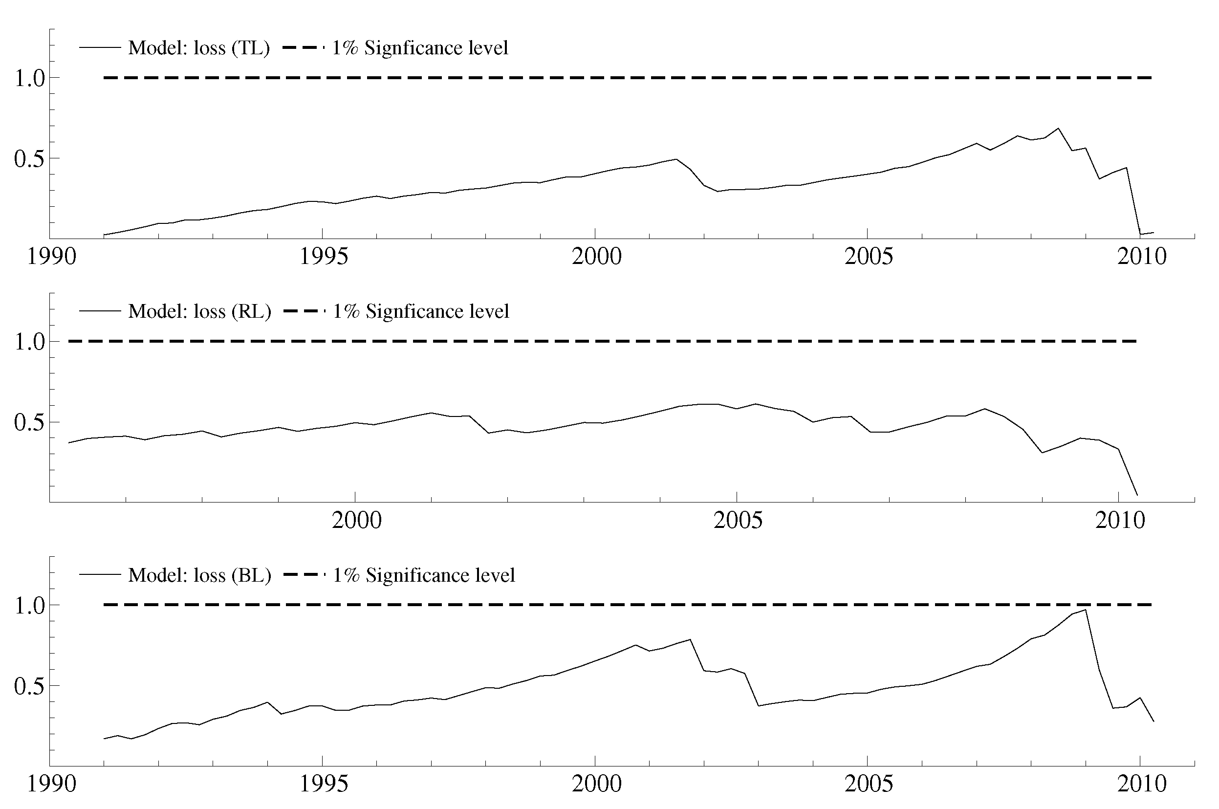
Table A2 also report the results of several misspecification tests. It can be seen from the table that the residuals of the three models are reasonably well behaved. While there are still some signs of auto-correlation, in particular in the model for real estate losses, the effect on the results are nevertheless likely to be minor. Also, the normality assumption is rejected at the 5% significance level in all three models due to a few outliers. To investigate the parameter stability of the models, Figure A1 shows the results from recursive break-point Chow tests. Values above the black dotted line indicate rejection of parameter stability at the 1% significance level. As can be seen from the figure, all three models seem to display reasonable parameter stability.

Table A2.
Estimated transition parameters and regime coefficients from dynamic versions of the STR models for the credit loss rates. Boldface values indicate significance at the 5% level (standard errors in parenthesis). The null hypothesis of no auto-correlation (AR) in up to five lags of the residual is tested by a Lagrange multiplier test. A similar test is conducted on the squared residuals to test for the null of no auto-regressive conditional heteroscedasticity (ARCH). The last row reports the adjusted coefficient of determination.
| Dynamic STR Estimates | |||
|---|---|---|---|
| Model | |||
| Explained: | |||
| Parameters | |||
| – | |||
| – | |||
| Misspecification | |||
| AR | |||
| ARCH | |||
| Normality | |||
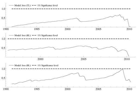
Figure A1.
Parameter stability tests. The black solid lines depict recursive break-point Chow tests for the models in Table A2. Twenty quarters were used to initialize the recursions. Values above the dotted black line indicate rejection of parameter stability at the 1% significance level.
Figure A1.
Parameter stability tests. The black solid lines depict recursive break-point Chow tests for the models in Table A2. Twenty quarters were used to initialize the recursions. Values above the dotted black line indicate rejection of parameter stability at the 1% significance level.
As a final assessment of the model, we compare the results in Table 4, which are based on the STR specification in (2), with an analogous MS model. In particular, the latter model has exactly the same explanatory variables and two regimes, but replaces the transition function, , with a unobserved random variable which follows a Markov chain. Hence, comparing the two models allows us to assess the benefits of having the financial obligations ratio as a specific transition variable: if the two model yield identical regimes, the value added of conditioning on this variable is limited. The estimates, of the MS-model (available upon request) are qualitatively in line with the ones for the STR model in Table 4, i.e., the effects of the cyclical variables are generally insignificant in Regime 1 and significantly negative in Regime 2. As a first statistical assessment of the MS model, we check if it produces stationary residuals for each of the three loss rates. The ADF-test statistics on the residuals of , , and are −2.66, −3.25, and −4.73, respectively. This implies that we cannot reject the unit-root hypothesis for the residuals of the equation for the loss rate on total loans. For the loss rate on real estate loans we reject this hypothesis at the 5%, but not on the 1% significance level, whereas the residual of the equation for losses on business loans is clearly stationary. In all three cases, however, the residual persistence of the STR model is less than that of the MS model.
Figure A2 depicts the weights to (or probabilities of) Regime 2 which are implied by the STR and MS models. While the two types of models yield transitions between regimes which are broadly reminiscent of each other, there are nevertheless several sharp differences as is clear from the figure. The most wide dispersion between the regimes is obtained with respect to the models for losses on total loans (upper panel). The regime classification of the MS model for this loss rate, does not seem to be entirely reasonable. In particular, the episodes in the “bad” regime which are associated with the crisis periods in the early 1990s and late 2000s are very long, for instance starting the the late 1999’s for the latter crisis. Moreover, the strength of Regime 2 declines just prior to the crisis. These results indicate that the MS model for losses on total loans may not be able to characterize the data adequately, which is also evidenced by the failure to reject the unit-root hypothesis for the residuals of this equation. Turning to the models for the two remaining loss rates, we see that the transition patterns are more closely aligned. However, there is a clear tendency for the STR regimes to increase and decline approximately one year before the MS regimes. The only exception to this pattern is during the early 90’s recession in the model for losses on real estate loans, where the MS transition moves more sharply around the crisis date than the one obtained from the STR model.

Figure A2.
Estimated weights/probabilities to Regime 2 implied by the STR and the MS models.
Figure A2.
Estimated weights/probabilities to Regime 2 implied by the STR and the MS models.
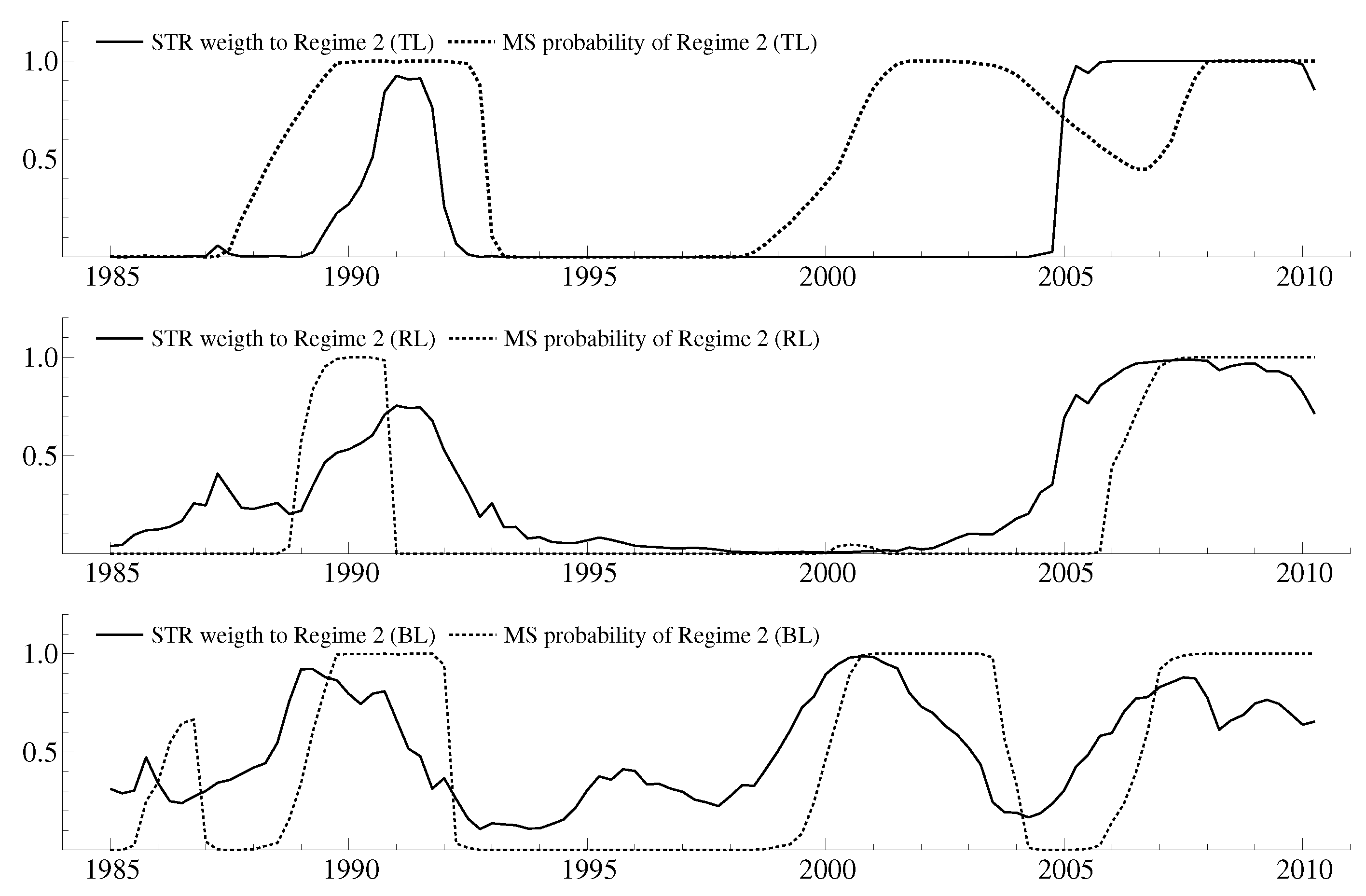
Taken together, these results point to substantial differences between the predictions of the two types of models. While the STR model is more demanding, as it requires successful specification of the transition variable, it nevertheless delivers significant pay-offs in terms of statistical fit, early warnings, and economic interpretation.
References
- Altunbas, Yener, Leonardo Gambacorta, and David Marques-Ibanez. 2010. Does Monetary Policy Affect Bank Risk-Taking? BIS Working Papers. No. 298. Available online: http://www.bis.org/publ/work298.htm (accessed on 6 November 2012).
- Berger, Allen N., Marco A. Espinosa-Vega, Nathan H. Miller, and W. Scott Frame. 2005. Debt maturity, risk, and asymmetric information. The Journal of Finance 60: 2895–923. [Google Scholar] [CrossRef]
- Bernanke, Ben S., Mark Gertler, and Simon Gilchrist. 1999. The financial accelerator in a quantitative business cycle framework. In Handbook of Macroeconomics. Edited by John B. Taylor and Michael Woodford. Amsterdam: North-Holland, vol. 1. [Google Scholar]
- Borio, Claudio. 2009. Implementing the macroprudential approach to financial regulation and supervision. Banque de France Financial Stability Review 13: 31–41. [Google Scholar]
- Borio, Claudio, and Mathias Drehmann. 2009. Assessing the risk of banking crises-revisited. BIS Quarterly Review. March. Available online: http://www.bis.org/publ/qtrpdf/r_qt0903e.htm (accessed on 6 November 2012).
- Borio, Claudio, and Philip Lowe. 2002. Asset prices, financial and monetary stability: Exploring the nexus. BIS Working Papers. No. 114. Available online: http://www.bis.org/publ/work114.htm (accessed on 6 November 2012).
- Burnside, Craig, Martin Eichenbaum, and Sergio Rebelo. 2016. Understanding booms and busts in housing markets. Journal of Political Economy 124, 4: 1088–147. [Google Scholar] [CrossRef]
- Caballero, Ricardo J., Emmanuel Farhi, and Pierre-Olivier Gourinchas. 2008. An equilibrium model of "global imbalances" and low interest rates. American Economic Review 98: 358–93. [Google Scholar] [CrossRef]
- Campello, Murillo, John R. Graham, and Campbell R. Harvey. 2010. The real effects of financial constraints: Evidence from a financial crisis. Journal of Financial Economics 97: 470–87. [Google Scholar] [CrossRef]
- Choi, In, and Pentti Saikkonen. 2004. Testing linearity in cointegrating smooth transition regressions. Econometrics Journal 7: 341–65. [Google Scholar] [CrossRef]
- Dell’Ariccia, Giovanni, and Robert Marquez. 2006. Lending booms and lending standards. The Journal of Finance 61: 2511–46. [Google Scholar] [CrossRef]
- Drehmann, Mathias, Claudio Borio, Leonardo Gambacorta, Gabriel Jiménez, and Carlos Trucharte. 2010. Countercyclical capital buffers: Exploring options. BIS Working Papers. No. 317. Available online: http://www.bis.org/publ/work317.htm (accessed on 6 November 2012).
- Drehmann, Mathias, and Mikael Juselius. 2012. Do debt service costs affect macroeconomic and financial stability? BIS Quarterly Review. September. Available online: http://www.bis.org/publ/qtrpdf/r_qt1209e.htm (accessed on 6 November 2012).
- Dynan, Karen, Kathleen Johnson, and Karen Pence. 2003. Recent changes to a measure of US household debt service. Federal Reserve Bulletin 89: 417–26. [Google Scholar]
- Frydman, Roman, and Michael D. Goldberg. 2009. Financial markets and the state: Price swings, risk, and the scope of regulation. Capitalism and Society 4: 1–43. [Google Scholar] [CrossRef]
- Gai, Prasanna, Sujit Kapadia, Stephen Millard, and Ander Perez. 2008. Financial innovation, macroeconomic stability and systemic crises. The Economic Journal 118: 401–26. [Google Scholar] [CrossRef]
- Gertler, Mark, and Cara S. Lown. 1999. The information in the high-yield bond spread for the business cycle: Evidence and some implications. Oxford Review of Economic Policy 15: 132–50. [Google Scholar] [CrossRef]
- Gilchrist, Simon, Vladimir Yankov, and Egon Zakrajšek. 2009. Credit market shocks and economic fluctuations: Evidence from corporate bond and stock markets. Journal of Monetary Economics 56: 471–93. [Google Scholar] [CrossRef]
- Hall, Robert. 2011. The long slump. American Economic Review 101, 2: 431–69. [Google Scholar] [CrossRef]
- Iacoviello, Matteo. 2005. House prices, borrowing constraints, and monetary policy in the business cycle. American Economic Review 95: 739–64. [Google Scholar] [CrossRef]
- Johansen, Søren. 1996. Likelihood-Based Inference in Cointegrated Vector Auto-Regressive Models. Oxford: Oxford University Press. [Google Scholar]
- King, Mervyn. 1994. Debt deflation: Theory and evidence. European Economic Review 38: 419–55. [Google Scholar] [CrossRef]
- Kiyotaki, Nobuhiro, and Mark Gertler. 2010. Financial intermediation and credit policy in business cycle analysis. In Handbook of Monetary Economics. Edited by Benjamin M. Friedman and Michael Woodford. Amsterdam: Elsevier. [Google Scholar]
- Kiyotaki, Nobuhiro, and John Moore. 1997. Credit cycles. Journal of Political Economy 105: 211–48. [Google Scholar] [CrossRef]
- Leybourne, Stephen, Paul Newbold, and Dimitrios Vougas. 1998. Unit roots and smooth transitions. Journal of Time Series Analysis 19: 83–97. [Google Scholar] [CrossRef]
- Lorenzoni, Guido. 2008. Inefficient credit booms. Review of Economic Studies 78: 809–33. [Google Scholar] [CrossRef]
- Meier, Andre, and Gernot J. Müller. 2006. Fleshing out the monetary transmission mechanism: Output composition and the role of financial frictions. Journal of Money, Credit, and Banking 38: 2099–133. [Google Scholar] [CrossRef]
- Mian, Atif, and Amir Sufi. 2010. The great recession: Lessons from microeconomic data. American Economic Review 100: 1–10. [Google Scholar] [CrossRef]
- Miller, Marcus, and Joseph E. Stiglitz. 2010. Leverage and asset bubbles: Averting armageddon with chapter 11? The Economic Journal 120: 500–18. [Google Scholar] [CrossRef]
- Nelson, Charles R., Jeremy Piger, and Eric Zivot. 2001. Markov regime switching and unit-root tests. Journal of Business & Economic Statistics 19: 404–15. [Google Scholar]
- Repullo, Rafael, Jesus Saurina, and Carlos Trucharte. 2010. Mitigating the pro-cyclicality of Basel II. Economic Policy 25: 659–702. [Google Scholar] [CrossRef]
- Ruckes, Martin. 2004. Bank competition and credit standards. The Review of Financial Studies 17: 1073–102. [Google Scholar] [CrossRef]
- Saikkonen, Pentti, and In Choi. 2004. Cointegration smooth transition regressions. Econometric Theory 20: 301–40. [Google Scholar] [CrossRef]
- Saikkonen, Pentti, and In Choi. 2010. Tests for nonlinear cointegration. Econometric Theory 26: 682–709. [Google Scholar]
- Stein, Jerome L. 2006. Stochastic Optimal Control, International Finance, and Debt Crises. Oxford: Oxford University Press. [Google Scholar]
- Stohs, Mark Hoven, and David C. Mauer. 1996. The determinants of corporate debt maturity structure. The Journal of Business 69: 279–312. [Google Scholar] [CrossRef]
- Van Dijk, Dick, Timo Teräsvirta, and Philip Hans Franses. 2002. Smooth transition autoregressive models—A survey of recent developments. Econometric Reviews 21: 1–47. [Google Scholar] [CrossRef]
| 1. | Several empirical studies also attempt to quantify the relative importance of the financial accelerator for output fluctuations. See for instance, Gertler and Lown (1999), Meier and Müller (2006), Gilchrist et al. (2009), and references therein. |
| 2. | The temporal association between credit losses and output losses is very strong as can be seen by comparing panels (a) and (e) of Figure 1. |
| 3. | This conjecture has recently been corroborated in a subsequent paper by Drehmann and Juselius (2012), who construct debt service ratios, a more narrow counterpart to the financial obligations ratio, for 27 countries. They find that the debt service ratio produce more accurate early warning signals than other extant measures 1–2 years ahead of systemic banking crises, whereas the credit-to-GDP gap have superior performance at longer horizons. |
| 4. | See the Federal Financial Institutions Examination Council’s “Instructions for Preparation of Consolidated Reports of Condition and Income (FFIEC 031 and 041)” and the Generally Accepted Accounting Principles (GAAP). |
| 5. | In the empirical analysis, we also control for a number of other variables including real house prices, deviations from a standard Taylor’s rule, the real exchange rate, the unemployment rate, and the inflation rate. |
| 6. | The numerator also includes rent payments on tenant-occupied property, auto lease payments, homeowners’ insurance, and property tax payments. |
| 7. | This value lies between the average maturities on firms’ bank loans reported in Stohs and Mauer (1996) and Berger et al. (2005). We checked robustness of the results below by assuming 2 and 4 years maturities. The results did not change significantly and are available upon request. |
| 8. | The precision with which the critical thresholds can be estimated depends more on the relative number of observations in each regime than the number of transitions between regimes. For instance, while our sample contains only two episodes of severe household sector financial distress, the number of observations associated with these events is 34, i.e., approximately one third of the entire sample. |
| 9. | Both the output gap and the term structure should be stationary. Moreover, credit losses reduce the credit aggregates so that even if they affect output debt to GDP ratios would not move too much. |
| 10. | See Saikkonen and Choi (2004) for a discussion of this model. |
| 11. | We also tried the other variables in , as well as real house prices. None, of these variables produced superior results in the sense discussed in Section 4.2. |
| 12. | The only exception is the financial obligations ratio on total business loans which is found to be stationary. These results are available upon request. |
| 13. | These results are omitted for brevity, but are available upon request. We also tried per capita GDP, the inflation rate, the unemployment rate, and the real exchange rate. None of these were found to be both cointegrated and weakly exogenous with respect to the credit loss rates. |
| 14. | This is statistically justified if the federal funds rate is strongly exogenous and the Hodrick-Prescott filtered trend provides an accurate estimate of the underlying trend in the federal funds rate. We found some evidence in favor of strong exogeneity for the federal funds rate by testing additional restrictions on the short-term dynamics. While there is no guarantee that the Hodrick-Prescott trend is an accurate estimate of the underlying trend, we checked robustness by estimating (2) with on the left hand side and added to the right hand side. This does not change the results below to any significant degree. |
| 15. | This does not, however, imply that such shifts are not present in the pre-crisis sample, but rather that the resulting dynamics are of a lesser magnitude and, hence, not likely to be confused with long-run movements in the credit loss rates. |
| 16. | Applying a more appropriate test, such as the one in Saikkonen and Choi (2010) which is based on the KPSS test, is left for future work. |
| 17. | It is more difficult to conduct a similar test for the household sector, as the Federal Reserve does not record financial obligations ratios before 1985. |
© 2017 by the authors. Licensee MDPI, Basel, Switzerland. This article is an open access article distributed under the terms and conditions of the Creative Commons Attribution (CC BY) license (http://creativecommons.org/licenses/by/4.0/).

