1. Introduction
A time series can have multiple breaks. For example, U. S. Treasury bill rates can be observed to have multiple level changes over time, while the Grilli and Yang primary commodity price index shows multiple trend shifts. It is common that the number of breaks is unknown and misspecified. Bai (1995, 1997) [
1,
2] and Chong (1994, 1995) [
3,
4] study the consequences of underspecifying the number of break points in linear structural break models. They point out that when the number of breaks in a mean shift model is underspecified, the break point estimator is still consistent for a subset of the true break points. Their discussion covers the mean shift model with and without trend. Bai (1997) [
2] shows that the mean break point estimator by sequential estimation is not only consistent but also converges at the same rate as with simultaneous estimation. Bai and Perron (1998) [
5] extend the estimation of a single unknown break to multiple unknown breaks under both fixed and shrinking shift magnitudes. Based on the consistency property of the mean shift break point estimator, they propose a sequential procedure for multi-break estimates without estimating the multiple breaks simultaneously. Dynamic programming is introduced by Bai and Perron (2003) [
6] to deal with the computational burden in multiple break point estimation. Kejriwal and Perron (2010) [
7] extend the work of Perron and Yabu (2009) [
8,
9] to propose a sequential test of the multiple-trend-shift model robust to persistence in noise.
Although trending components are considered by researchers in the mean shift model, there is little discussion of the consistency of multiple trend shift break point estimators when the number of breaks is underspecified. Consistency analysis is important both for break point estimation and for structural breaks in the linear regression model. The main motivation of this paper is to address the gap in the literature concerning the consistency of trend shift break point estimators when the break number is underspecified.
The second motivation of this paper is to explore how to approximate the finite sample distributions of the break point estimator for a multiple break model. Specifically, asymptotics of the break point estimator in a trend shift model are provided for the case of an underspecified break number by employing Pitman drifts. The accuracy of the asymptotic approximation to the finite sample distribution is examined. This work follows Yang (2012) [
10] who has shown that the finite sample distribution of the single break point estimator is not normal, but depends on the break dates and magnitudes.
In this paper, finite sample simulations are used to illustrate the potential inconsistency of the break point estimator in the trend shift model with an underspecified break number. Then, the limits of the break point estimator under fixed break magnitudes are provided. Both the simulation results and the expression of the limits show that for the trend shift model, the break point estimator can be inconsistent for any of the true break points, while for the mean shift model, the break point estimator converges to one of the true breaks. Then, extending Yang’s (2012) work [
10] on the single break point estimator, new asymptotics are provided for the break point estimators under local alternatives.
As will be shown in this paper, the mean shift model leads to a consistent break point estimator while the trend shift model does not. Taking first differences of the trend shift model is shown by Yang (2010) [
11] to provide a solution to the inconsistency problem. When the break magnitudes are sufficiently large, the first-difference break point estimator has much higher peaks in the density at the true breaks than the levels break point estimator. When the break magnitudes are small, the densities of the two break point estimators depend on the break magnitudes and locations and the strength of the serial correlation. A detailed analysis of the first-difference estimator is omitted in this paper but can be found in Yang (2010) [
11] and Yang (2012) [
10].
The paper is organized as follows.
Section 2 describes the general settings of the mean shift and trend shift models, assumptions, and break point estimators.
Section 3 introduces finite sample simulations to demonstrate the consistency properties of different break point estimators.
Section 4 derives the expression of the limits of the single break point estimator when the break sizes are fixed and the data sequences have two breaks under I(0) errors. Both mean shift and trend shift break point estimators are discussed.
Section 5 establishes the asymptotic distributions of the break point estimators assuming the breaks are Pitman drifts, which approximate the finite sample distributions accurately.
Section 4 and
Section 5 relate the mean shift results to those of Bai (1997) [
2]. The last section concludes the paper. Proofs are provided in the
Appendix.
2. The Models, Assumptions, and Break Point Estimators
In this section, I define a mean shift and a trend shift model with multiple breaks. For simplicity, I only include the case where a single break model is estimated while the number of breaks is two. The results can be extended to models with more than two breaks.
Let us start with a mean shift model with two breaks:
where
and
are the true break fractions with
and
;
denotes the time of a break.
T is the sample length;
and
are the break magnitudes. For convenience of discussion, we define the relative break magnitude ratio
.
When model (
1) is underspecified, the estimated model is given by
where
λ is the underspecified single break fraction with
.
For comparison, the trend shift model with two breaks is
where
,
.
If model (
3) is misspecified with only one break, the estimated model is
where
.
It is assumed that the error
is I(0), namely
where
L is the lag operator;
is a martingale difference sequence with
,
, and
.
The break point estimators are obtained by minimizing the sum of squared residuals (SSR) over the trimming set
, namely
where
with
and
the OLS estimators from model (
2) with no restrictions imposed, whereas
,
, and
are the OLS estimators from model (
4) with no restrictions imposed.
3. Illustration of the Inconsistency Problem of the Trend Shift Break Point Estimator
In this section a simple simulation is used to illustrate the consistency/inconsistency of
and
in the presence of an underspecified break number. The data are generated based on models (
1) and (
3) with two breaks, where
T = 100, 250, 500, 1000,
,
ν = −2, −1, 1, 2 (we set
without loss of generality), and
is an
i.i.d. process. Equations (
6) and (7) are used to estimate
and
separately in each replication. While trimming is not necessary, to ensure the invertibility of the regression matrix I use 2% trimming, i.e.,
. The replications
N = 20,000, 10,000, 5000, 2500 are used for
T = 100, 250, 500, 1000 respectively.
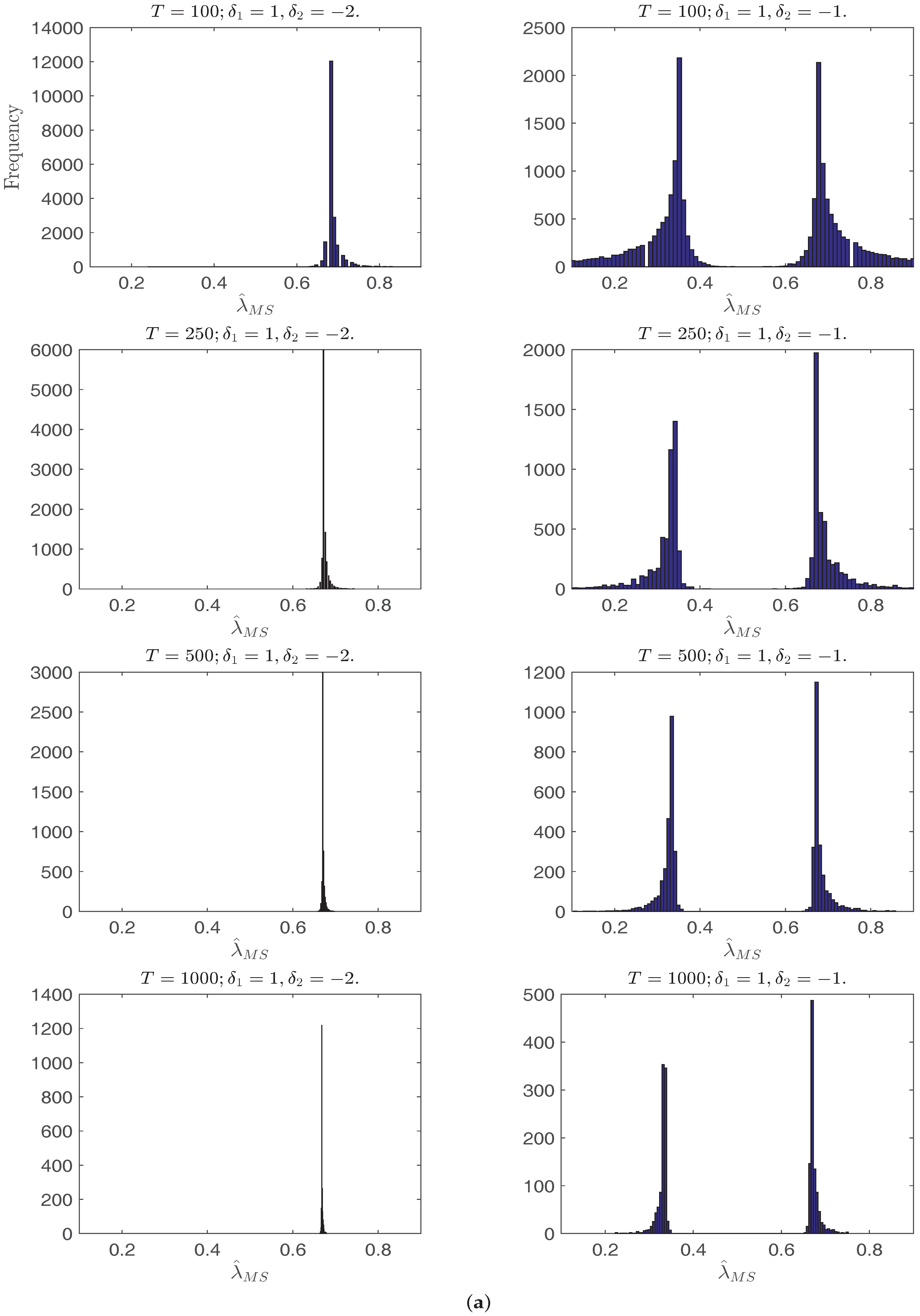
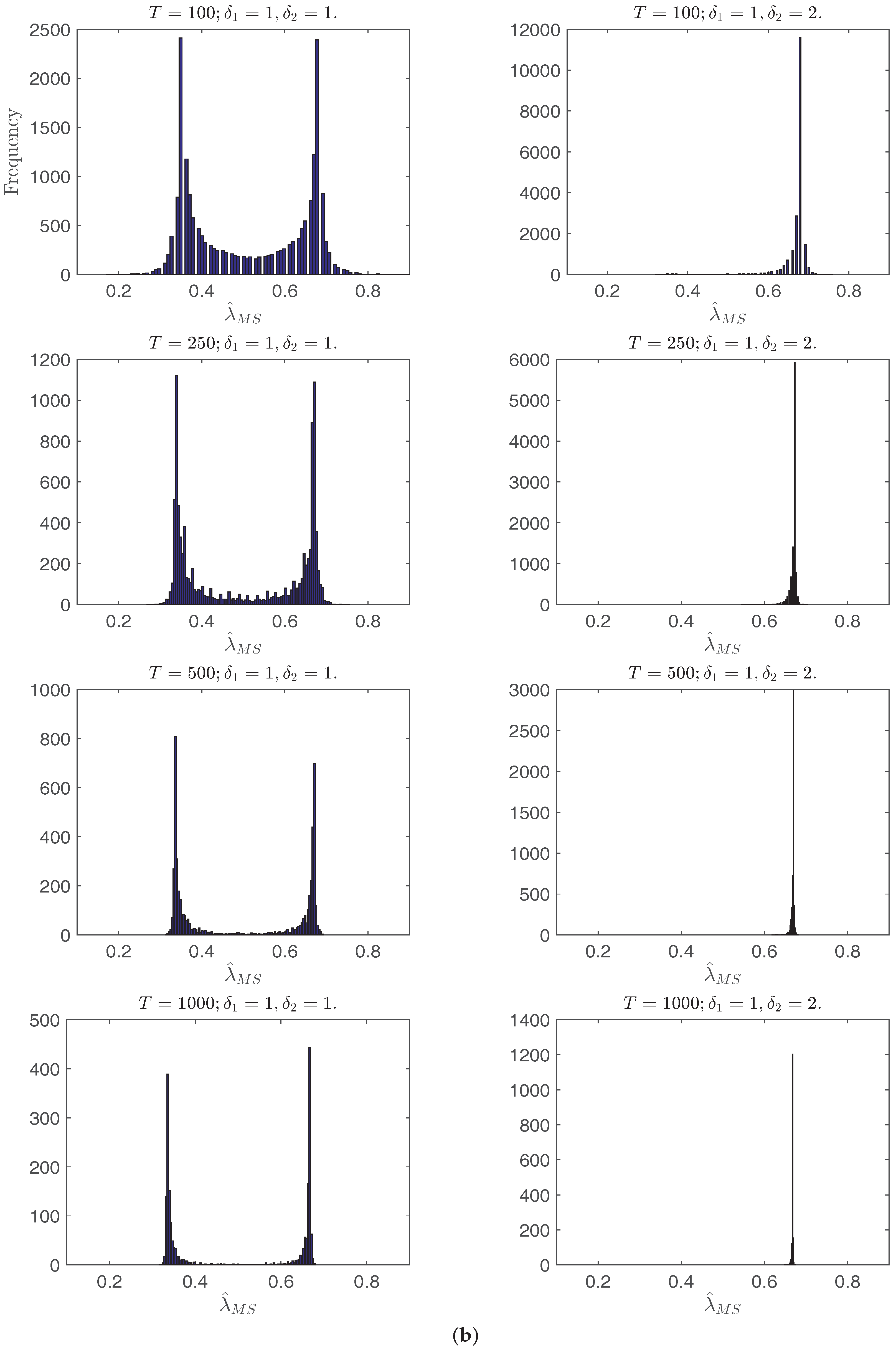
Figure 1a,b plots the histograms of
with
i.i.d. errors. In all cases with the increase of
T, the distribution of
has shorter tails and, when
, concentrates at the two break points or one of them depending on the relative break magnitude ratios. Interestingly, when
and
, the density of
is bimodal, which can be explained by Yang (2012) [
10] through the behavior of the mean shift break point estimator, where the break point estimates concentrate around the end points in the no break model.
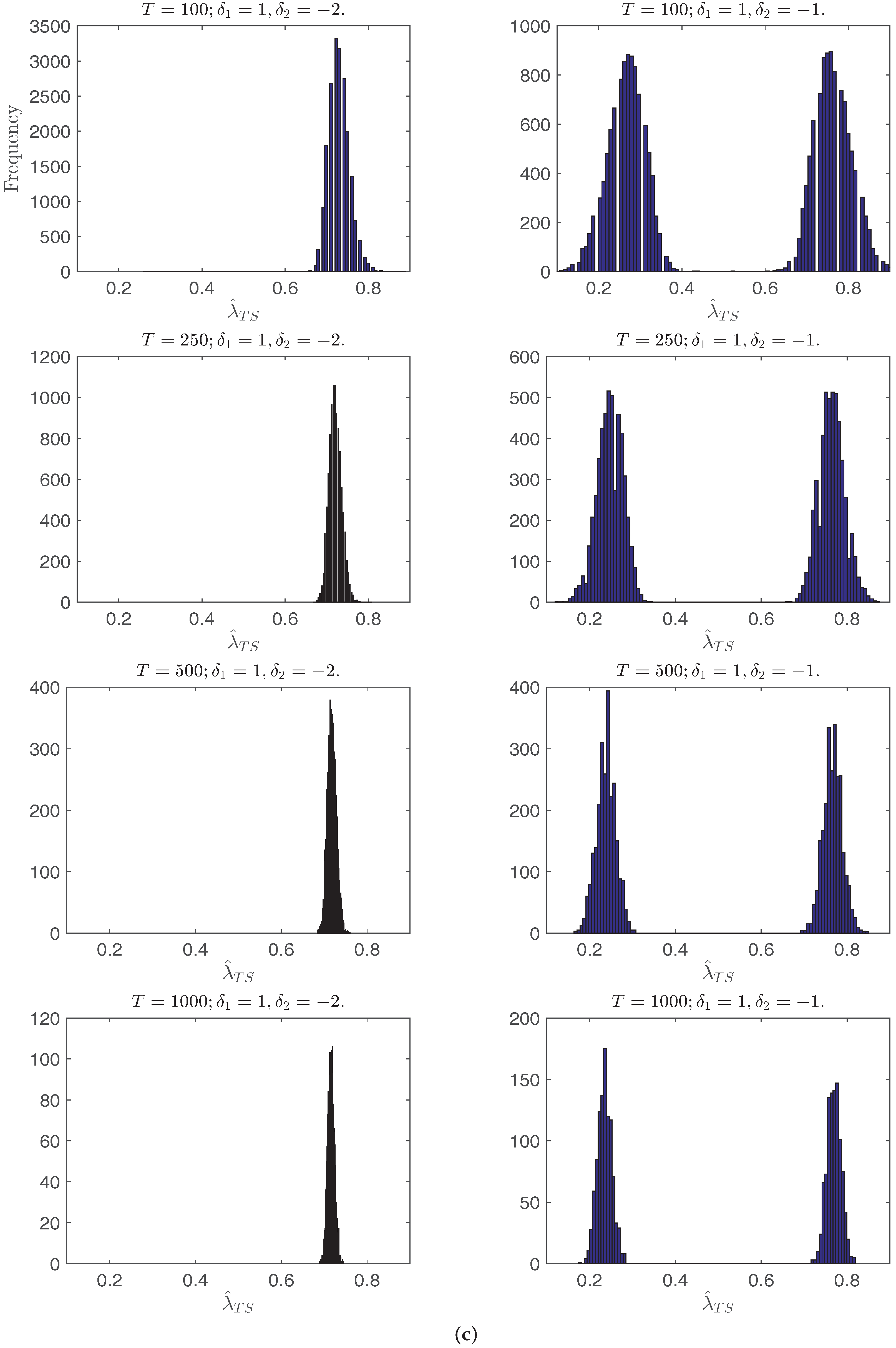
Figure 1c,d plots the histograms of
. When
, the density peaks at a point greater than
. When
,
has two equal peaks at
and
. When
, the histogram of
has only one peak at
, and with the increase of
T the break date estimates are more concentrated. When
, the histogram of
peaks at a point between
and
. This shows that when the number of breaks is underspecified, the trend shift break point estimator does not converge to either of the true break points, and that the limit of the break point estimator
depends on the break magnitudes and locations.
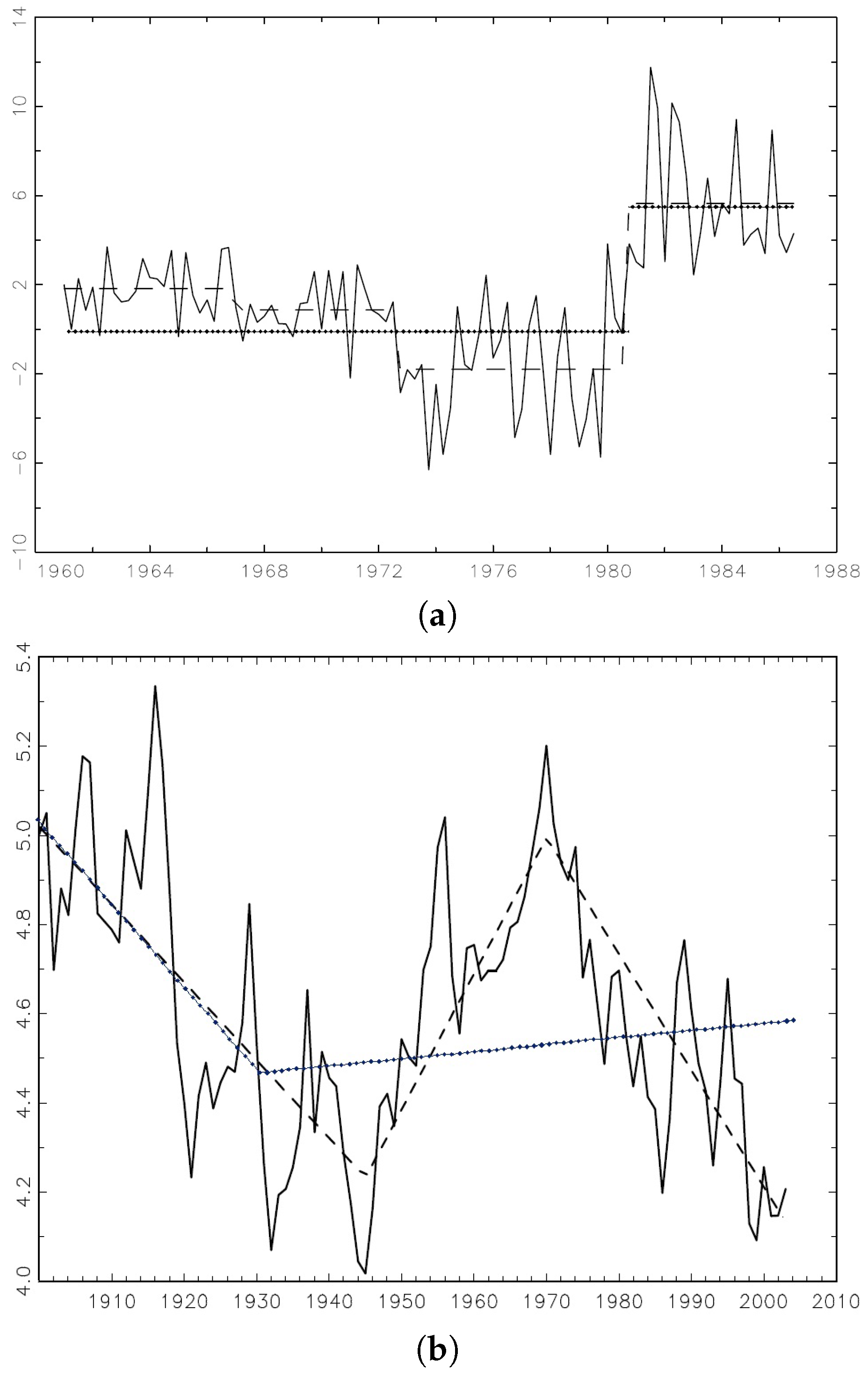
Empirical data also shows that the break point estimators behave differently when the break number is underspecified in mean shift model and trend shift model. Using the US ex-post real interest rate in
Figure 2 as an example of mean shifts (the three-month treasury bill rate between the first quarter of 1961 and the third quarter of 1986 deflated by the CPI inflation rate taken from the Citibase data bank), Bai and Perron (1998) [
5] detect three mean shifts in years 1965, 1972, and 1980 while a single mean shift point estimator detects one of the real breaks in 1980. Using the extended Grilli and Yang commodity price index as an example of trend shifts (Copper during 1900–2003), Harvey, Leybourne, and Taylor (2009) [
12] identify two breaks in 1945 and 1971, while a single trend shift estimator identifies one in 1930, which is not close to the HLT dates.
Both the finite sample histograms and empirical data suggest an interesting pattern: when the break number is underspecified, the mean shift break point estimator converges to a subset of the true break points, while the trend shift counterpart does not converge to either of the true break points and its limit depends on the break dates and magnitudes.
4. Limits of the Break Point Estimators when the Break Magnitudes are Fixed
Similar to the discussion in Bai (1997) [
2] for the mean shift results, the limits of the single trend break point estimator
are derived in this section when the break sizes are fixed and the data sequences have two trend breaks.
Theorem 1. Assume there are two break fractions and with fixed break magnitudes in models (1) and (3) while the break number is underspecified as one.- 1.
For the mean shift model (1), under assumption (5) with fixed break magnitudes and , the break point estimator converges to one of the true breaks:where andEssentially - 2.
For the trend shift model (3), under assumption (5) with fixed break magnitudes and , the break point estimator has the following limit:where and
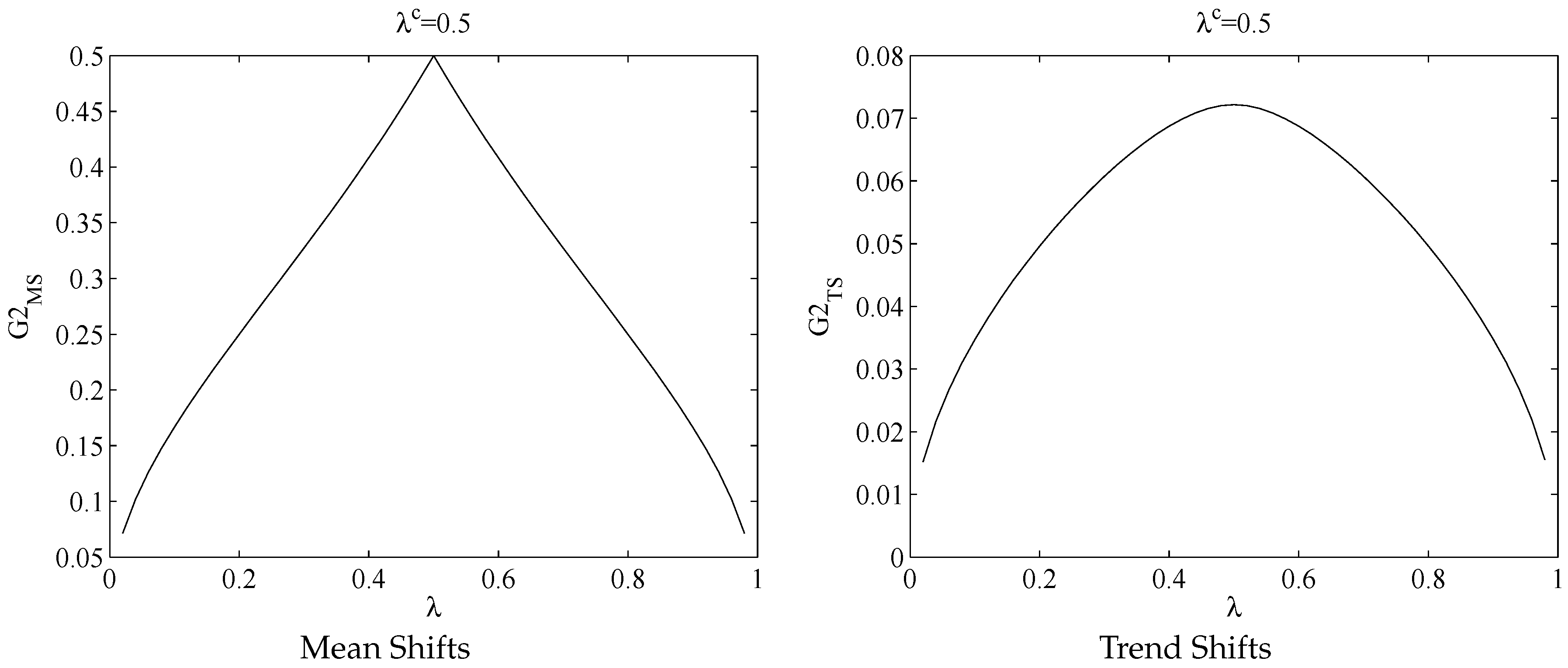
The limit of
is either
or
as shown in
Figure 3, which is consistent with the results in Bai (1997) [
2] using a different theoretical framework. Not surprisingly,
is maximized at
and
converges to one of the true break points.
The limit of
has different patterns. It is still true that
achieves a maximum at
as shown in
Figure 3. What makes it different from the mean shift case is when we sum up the two
terms, the function smooths out through the two peaks at each
. Hence, when the number of trend breaks is two while assumed to be one,
peaks neither at
nor at
.
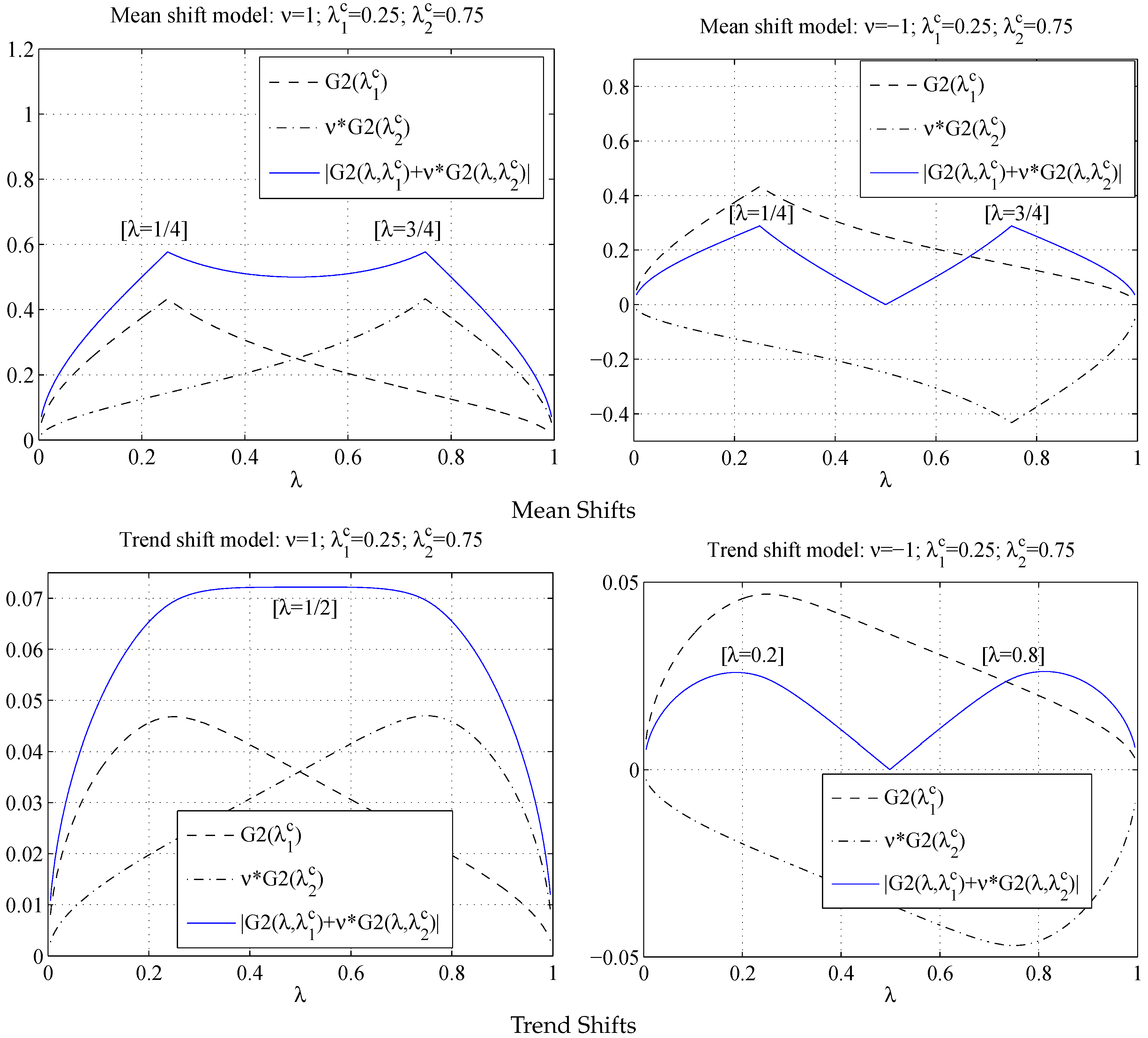
Figure 4 plots
with
and
and
. In both cases
peaks at neither of the true break points. Certainly, if
is smaller than 1,
will be closer to
; and if
is bigger than 1,
will be closer to
. This clearly explains the reason for the inconsistency of the trend shift break point estimator when the break number is underspecified.
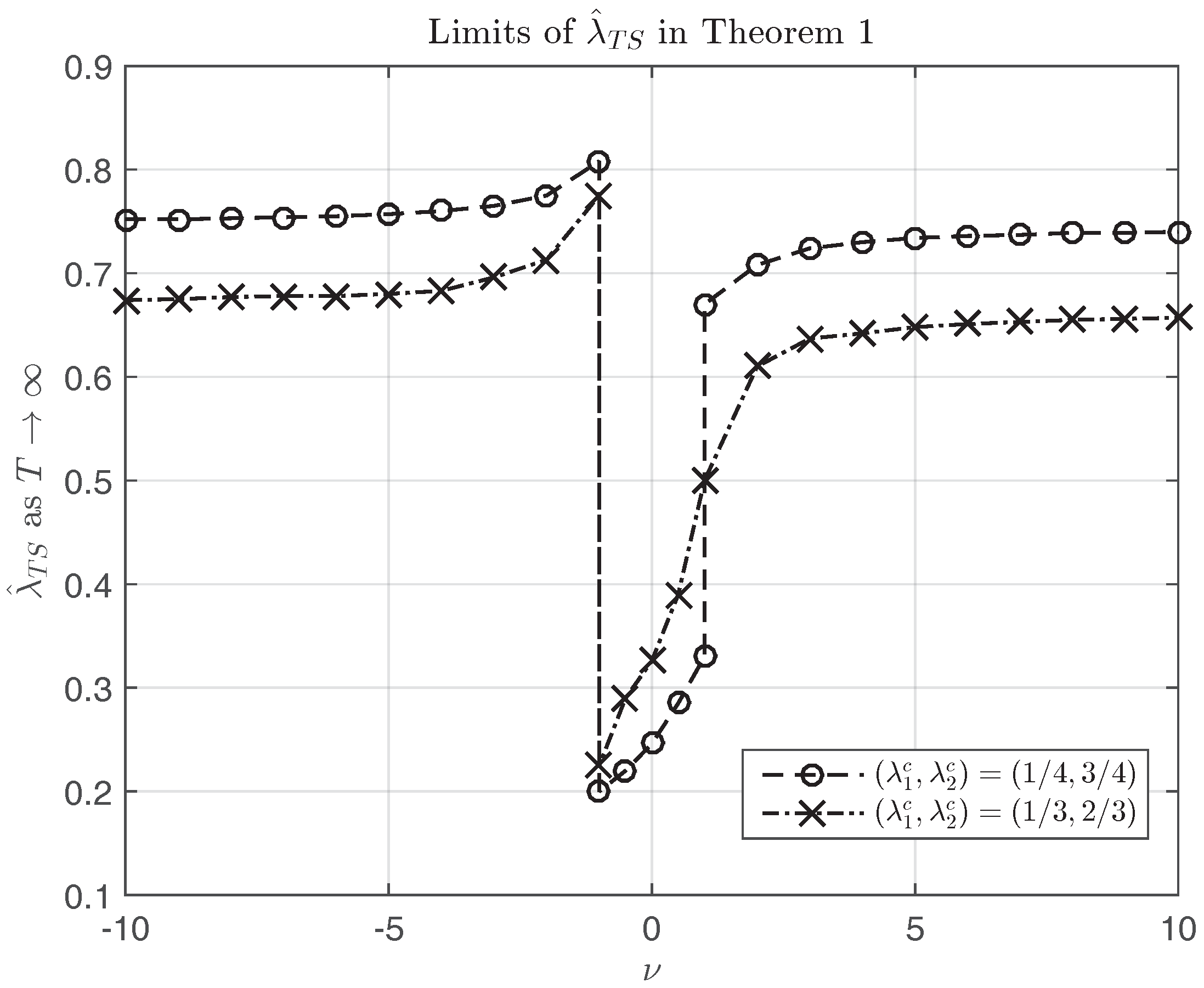
Figure 5 plots the
λ’s where
is maximized along
ν when
and
. When
,
is maximized at
. When
goes to ∞, the limit of the break point estimator will be the true break
. Other than these practically uninteresting cases, the limits of
will not be the true break points. Take
as an example. When
, the limiting point is greater than
. When
, the limiting point is less than
. In both cases, the limiting points are beyond the range of the two true breaks. When
, the limiting points are between the true breaks. When
, the limiting point is at
, the trend shift break point estimator is far away from the true breaks. As
ν goes away from 1, the limit of the trend shift break point estimator gets closer to one of the true breaks. The limits tell us the magnitude of the discrepancy between the spurious break and true breaks. Numerically when
or
, the limits of the spurious break point will be between
of the true breaks. This threshold can be extended to other cases with different break locations.
We summarize the findings on the consistency/inconsistency of
and
under assumption (
5) as follows:
For the mean shift model with two breaks, if the break magnitudes are not zero, the single break point estimator
is consistent for either
or
:
For the trend shift model
1 with two breaks, if the break magnitudes are not zero, the single break point estimator
is inconsistent for either
or
:
The limit depends on
,
, and
ν:
5. Limiting Distributions of and by Employing Pitman Drifts
As shown in the literature, asymptotic results derived under Pitman drifts often closely approximate the finite sample behavior of the test statistics or estimators involved. In the following, the limiting distributions of and are developed under Pitman drifts.
Theorem 2. Assume there are two break points and in the linear model while the break number is underspecified as one.- 1.
For the mean shift model (1), under assumptions (5) and and , where and are constant scalars, the break point estimator has the following limiting distribution:where , , and - 2.
For the trend shift model (3), under assumptions (5) and and , where and are constant scalars, the break point estimator has the following limiting distributions:where , , , and is defined in Theorem 1.
The asymptotics in Theorem 2 are an extension of work by Yang (2012) [
10] from the single-break case to the multiple-break case. To understand the effect of
,
,
, and
on the limiting distributions, I decompose the part inside the
in Equations (
11) and (
12) into three parts, where
For the asymptotic distribution of , with the form of in the limiting distributions, Theorem 2 provides a bridge between the asymptotics under the null of no breaks and the asymptotics under local alternatives of up to two breaks.
The asymptotics are continuous at
, i.e.,
and
could be as small as possible in the asymptotics. When
and
are small, the random component
dominates
and the distribution is close to the case of no breaks. For a small
M,
concentrates more around the middle range exhibiting a bell shape, while
concentrates more around the boundaries exhibiting a U shape. The detailed explanation is given in Yang (2012) [
10]. For a moderate
M, the limiting distribution of
exhibits a shape of W, resulting from the mixed effects of
and
in the asymptotics. If
, both
and
increase to ∞,
The limiting distributions in Theorem 2 are nonstandard. , , and show up in the approximations, and capture the effects of M’s and ’s on the asymptotics. Besides other deterministic variables in Theorem 2, the main random variables in the asymptotic distributions are functions of a Wiener process. The Wiener process in the asymptotic distributions was approximated by using standard normal i.i.d. random deviates. Integrals were approximated by normalized partial sums of 1000 steps using 10,000 replications.
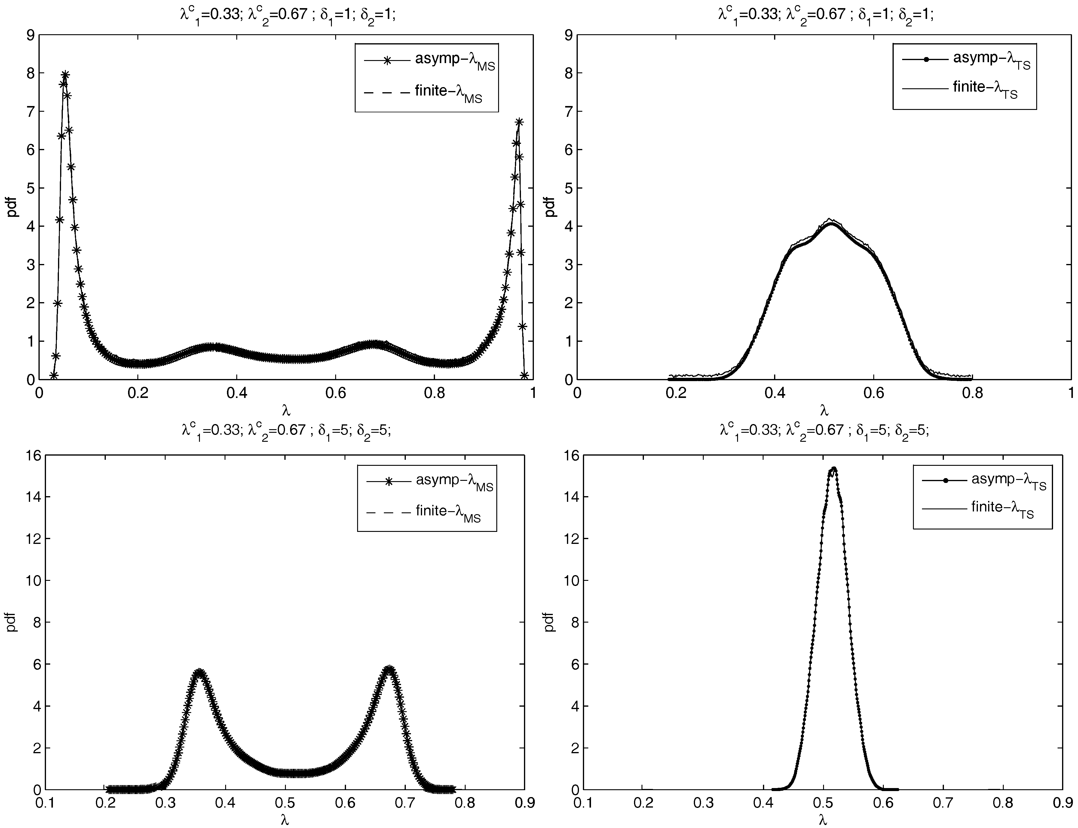
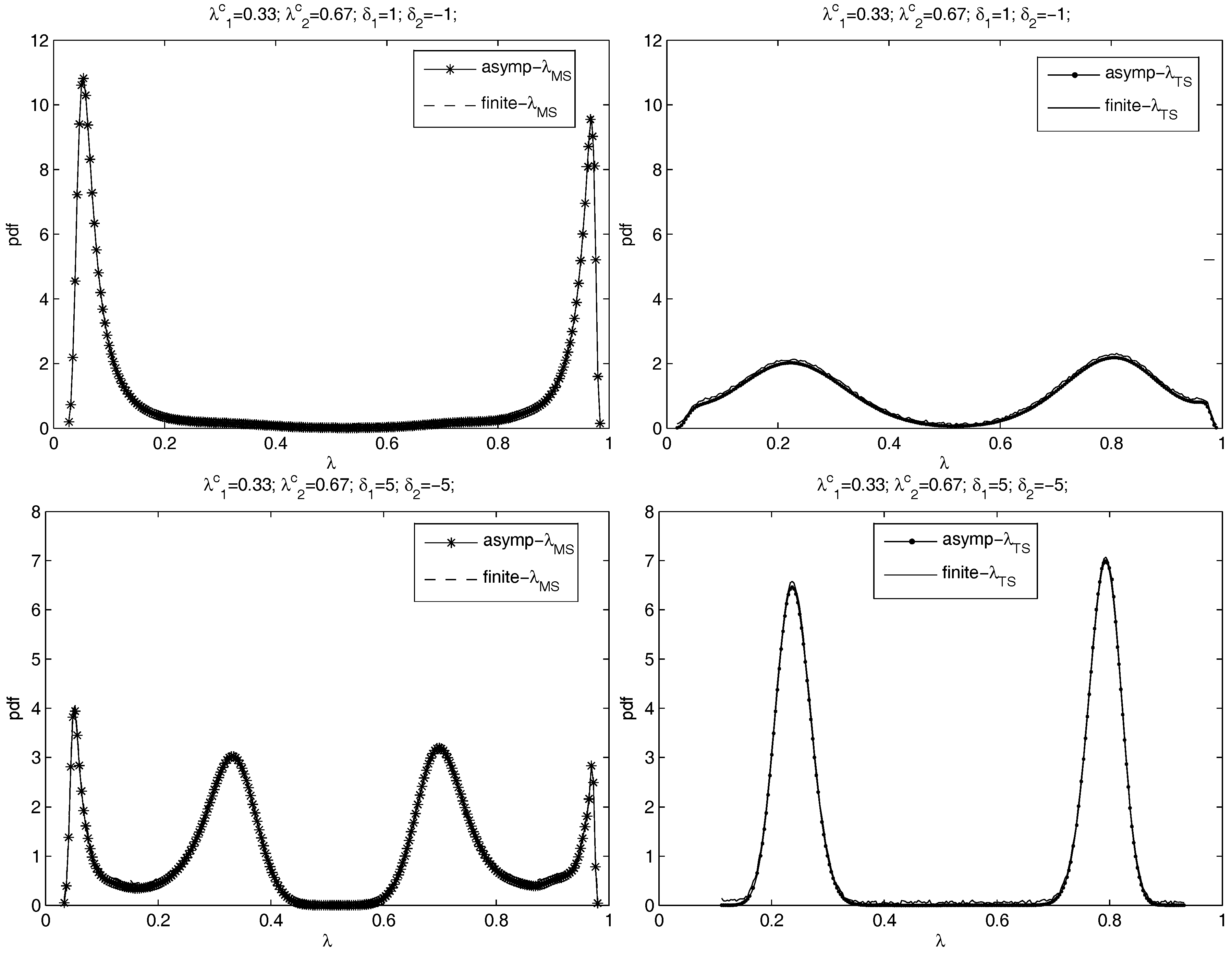
Figure 6 plots the finite sample distributions of
and
with
and asymptotic distributions for
,
. Errors are
i.i.d. . The left panels of
Figure 6 are for
and the right panels are for
. From the top to the bottom are the cases of
=
,
,
, and
. The pdfs of
and
are plotted in separated figures with the same scales to show the performance comparison in the presence of an underspecified break number. Kernel smoothing is used to obtain the pdf based on the simulations.
Figure 6 compares the asymptotic limits given by Theorem 2 to finite sample distributions. The two lines in each panel are near-identical, which shows that the asymptotics does a good job of approximating finite sample distributions of the break point estimators.
6. Conclusions
This paper analyzes the consistency of trend shift break point estimators when the number of breaks is underspecifed. The limit of the trend shift break point estimator for fixed break sizes is shown to be dependent on the break magnitudes and locations. In general, the trend shift break point estimator does not consistently estimate one of the true break points. Using the Pitman drift assumption, the limiting distribution of the trend shift break point estimator is shown to closely resemble the finite sample distributions.
Acknowledgments
I am very grateful to Tim Vogelsang for his continuous guidance and encouragement, and to Pierre Perron, two anonymous referees for their very helpful and constructive comments. I would also like to thank Mark Nichols and the participants at “The International Symposium on Recent Developments in Econometric Theory with Applications in Honor of Professor Takeshi Amemiya”.
Conflicts of Interest
The author declares no conflict of interest.
Appendix A.
Appendix A.1. Proof of Theorem 1
Theorem 1 can be proved simply by following the steps provided in the proof of Theorem 2 below.
Appendix A.2. Proof of Theorem 2
Appendix A.2.1. Asymptotic Distribution of
Let
be the SSR under the assumption of no breaks. Following Equation (
6), we obtain
The OLS estimator of
δ from (
2) is given by
where
and
are the residuals from the OLS regressions of
and
on
,
When the DGP is given by (
1), simple algebra gives
Multiplying both sides of the above equation by
, we have
Using
and
and
we obtain
where
From this result, it immediately follows that
Applying the CMT theorem gives
where
and
.
It is straightforward to show that
is maximized at either
or
. The first derivative of
w.r.t.
λ is given by:
Assume
, then it follows that
and
Through simple algebra, one can show that the peak values of
will be obtained at either
or
.
Appendix A.2.2. Asymptotic Distribution of
Let
be the SSR under the assumption of no breaks. From Equation (7), we have the standard result that
where
and
are the residuals from the OLS regressions of
and
on
.
When the DGP is given by (
3), simple algebra gives
Using
and
and
we obtain
From this results, it immediately follows that
Furthermore, using the CMT we obtain the limit of the break point estimator as
where
and
.
Please refer to Yang (2012) [
10] for more details about
and
.
References
- J.S. Bai. “Least absolute deviation estimation of a shift.” Econom. Theory 11 (1995): 403–436. [Google Scholar] [CrossRef]
- J.S. Bai. “Estimating multiple breaks one at a time.” Econom. Theory 13 (1997): 315–352. [Google Scholar] [CrossRef]
- T. Chong. Consistency of Change-Point Estimators When the Number of Change Points in Structural Change Models is Underspecified. Working Paper; Rochester, NY, USA: Department of Economics, University of Rochester, 1994. [Google Scholar]
- T. Chong. “Partial parameter consistency in a misspecified structural change model.” Econ. Lett. 49 (1995): 351–357. [Google Scholar] [CrossRef]
- J.S. Bai, and P. Perron. “Estimating and testing linear models with multiple structural breaks.” Econometrica 66 (1998): 47–78. [Google Scholar] [CrossRef]
- J.S. Bai, and P. Perron. “Computation and analysis of multiple structural change models.” J. Appl. Econom. 18 (2003): 1–22. [Google Scholar] [CrossRef]
- M. Kejriwal, and P. Perron. “A sequential procedure to determine the number of breaks in trend with an integrated or stationary noise component.” J. Time Ser. Anal. 31 (2010): 305–328. [Google Scholar] [CrossRef]
- P. Perron, and T. Yabu. “Estimating deterministic trends with an integrated or stationary noise component.” J. Econom. 151 (2009): 56–69. [Google Scholar] [CrossRef]
- P. Perron, and T. Yabu. “Testing for shifts in trend with an integrated or stationary noise component.” J. Bus. Econ. Stat. 27 (2009): 369–396. [Google Scholar] [CrossRef]
- J. Yang. “Break point estimators for a slope shift: levels versus first differences.” Econom. J. 15 (2012): 154–169. [Google Scholar] [CrossRef]
- J. Yang. “Essays on Estimation and Inference in Models with Deterministic Trends with and without Structural Change.” Ph.D. Thesis, Department of Economics, Michigan State University, East Lansing, MI, USA, 2010. [Google Scholar]
- D.I. Harvey, S.J. Leybourne, and A.M.R. Taylor. “Simple, robust and powerful tests of the breaking trend hypothesis.” Econom. Theory 25 (2009): 995–1029. [Google Scholar] [CrossRef]
1.If ’s are included together with ’s in model (3), under the condition of fixed break magnitudes, the trend shifts will dominate the mean shifts in the (in)consistency of the break point estimator, following the results in Theorem 1. If ’s are included in model (3), the slope change will force a large level shift. Under this condition, the consistency property of mean shifts will be dominant and the inconsistency problem in break point estimator will not persist anymore.
Figure 1.
Histograms of the single break point estimator or when and always. From top to bottom on each page: T = 100, 250, 500, 1000. (a) Histograms of when ; (b) Histograms of when ; (c) Histograms of when ; (d) Histograms of when .
Figure 1.
Histograms of the single break point estimator or when and always. From top to bottom on each page: T = 100, 250, 500, 1000. (a) Histograms of when ; (b) Histograms of when ; (c) Histograms of when ; (d) Histograms of when .
Figure 2.
Single break point estimate (dotted line) while multiple mean shifts or trend shifts exist (dashed line). (a) US ex-post real interest rate during Q1 1961–Q3 1986; (b) Primary commodity price index (Copper) relative to the price of manufacture during 1900–2003.
Figure 2.
Single break point estimate (dotted line) while multiple mean shifts or trend shifts exist (dashed line). (a) US ex-post real interest rate during Q1 1961–Q3 1986; (b) Primary commodity price index (Copper) relative to the price of manufacture during 1900–2003.
Figure 3.
and with .
Figure 3.
and with .
Figure 4.
for mean shift model and for trend shift model, where and −1, .
Figure 4.
for mean shift model and for trend shift model, where and −1, .
Figure 5.
Limits of in Theorem 1 when and along −10, ⋯, 10.
Figure 5.
Limits of in Theorem 1 when and along −10, ⋯, 10.
Figure 6.
The asymptotic distributions and the finite sample distributions of and when , , and is an i.i.d. process. The left: the distributions of ; the right: the distributions of . From the top to the bottom: = , , , and .
Figure 6.
The asymptotic distributions and the finite sample distributions of and when , , and is an i.i.d. process. The left: the distributions of ; the right: the distributions of . From the top to the bottom: = , , , and .
© 2017 by the author; licensee MDPI, Basel, Switzerland. This article is an open access article distributed under the terms and conditions of the Creative Commons Attribution (CC-BY) license ( http://creativecommons.org/licenses/by/4.0/).

